A Bearing Fault Diagnosis Method in Scenarios of Imbalanced Samples and Insufficient Labeled Samples

Abstract

In practical working environments, rolling bearings are one of the components that are prone to failure. Their vibration signal samples are faced with challenges, mainly including the imbalance between normal and fault samples as well as an insufficient number of labeled samples. This study proposes a sample-expansion method based on generative adversarial networks (GANs) and a fault diagnosis method based on a transformer to solve the above issues. First, selective kernel networks (SKNets) and a genetic algorithm (GA) were introduced to construct a conditional variational autoencoder–evolutionary generative adversarial network with a selective kernel (CVAE-SKEGAN) to achieve a balance between the proportion of normal and faulty samples. Then, a semi-supervised learning–variational convolutional Swin transformer (SSL-VCST) network was built for the fault classification, specifically introducing variational attention and semi-supervised mechanisms to reduce the overfitting risk of the model and solve the problem of a shortage of labeled samples. Three typical operating conditions were designed for the multi-case applicability verification. The results show that the method proposed in this study had good application effects when solving both sample imbalances and labeled-sample deficiencies and improved the accuracy of fault diagnosis in the above scenarios.

1. Introduction

Rolling bearings are susceptible to alternating loads, machining errors, and the impact of long-time operation, making them one of the parts prone to failure. The timely diagnosis of bearing failures is of great significance for the safety and work efficiency of equipment and personnel [1,2,3]. Deep-learning-based fault diagnosis models can learn deep fault characteristics from rolling bearings’ vibration signals and achieve high fault-diagnosis accuracy [4,5,6]. Convolutional neural networks (CNNs) [7] are representative of deep learning. Janssens et al. [8] used a CNN to identify bearing faults, which had a higher accuracy than traditional machine learning methods but was relatively limited in terms of global correlations and proved difficult to capture the relationship between distant pixels. However, transformer-based models [9,10] can learn the global feature representations in images, which compensates for the deficiency of a CNN in ultra-long period modeling. Huo et al. [11] proposed an improved transformer model with multiple self-attention mechanisms, which could better diagnose multiple faults in extreme class-imbalanced fault data. Yang et al. [12] proposed a signal transformer network based on a pure attention mechanism and demonstrated its effectiveness in feature extraction and fault identification in two sets of experiments. Although deep-learning-based fault diagnosis models have powerful feature-extraction capabilities, they highly rely on large-scale training samples [13,14,15].

In practical work environments, machines run normally most of the time, and there are fewer samples in a faulty state. Moreover, the cost of labeling fault samples is very expensive, resulting in a scarcity of labeled fault samples [16]. In this case, of an unbalanced ratio of normal and fault samples and insufficient labeled samples, deep-learning-based fault diagnosis models are prone to overfitting and lack good generalization ability and robustness, thus affecting the accuracy of a diagnosis [17]. Due to the fact that a transformer has almost no assumptions about the structural bias of the input data, it is difficult to apply one to small-scale labeled datasets [18]. Therefore, a transformer is usually combined with other methods to introduce a structural bias and solve the problem of insufficient labeled samples. Jin et al. [19] proposed a method to combine a time-series tokenizer and a transformer to achieve fault diagnoses. Wang et al. [20] proposed an automatic embedded transformer for fault diagnoses with few-shot data. Liu et al. [21] used convolutional layers to capture low-level local structural features, and transformers were used to segment patch sequences and model global dependencies for fault identification. Currently, how to use small-scale labeled datasets to train deep-learning models and achieve high-quality identification remains a challenge in fault-recognition research.

To address the problem of an imbalanced proportion of fault-free and fault samples, some researchers have combined generative adversarial networks (GANs) [22] and derivative models [23,24,25,26] to generate samples containing fault information to ensure the accuracy of deep-learning diagnostic models. To address the problem of a sample imbalance, Liang et al. [27] proposed a semi-supervised GAN framework, which utilized time–frequency images to diagnose single and compound faults in gears. Liu et al. [28] proposed an imbalance fault diagnosis method based on an improved multi-scale residual generative adversarial network and a feature-enhancement-driven capsule network, achieving enhanced performance in imbalanced-fault classification. Dixit et al. [29] combined model-agnostic meta-learning (MAML) with a conditional auxiliary classifier GAN (CACGAN) to initialize and update network parameters using MAML and then used conditional markers and auxiliary classifiers to generate samples. However, in the field of rolling-bearing fault diagnosis, the method of using a GAN to supplement data still has shortcomings in accurately learning data features and generating high-quality samples. Avoiding gradient vanishing and pattern collapse during model training is still a key challenge that urgently needs to be solved.

In summary, machine learning [30], feature engineering, deep learning [31], and transfer learning [32] are very important aspects of the prognostics and health management (PHM) of various fields, such as aerospace technology [33] and smart factories [34]. Aiming at the problems of a sample imbalance and a shortage of labeled samples, this study focuses on the sample expansion and fault-diagnosis methods of rolling bearings. A GAN and a transformer were adopted as the structural foundation of the network model. The main contributions of this study can be summarized as follows. First, we propose a sample-expansion method—namely, CVAE-SKEGAN—which solves the gradient-vanishing and mode-collapse problems of a GAN, giving it superiority in the stability and quality of the generated samples. Then, a novel rolling-bearing fault-diagnosis method, called SSL-VCST, is proposed. By optimizing the attention mechanism of the transformer and introducing semi-supervised training, unlabeled samples are fully utilized to improve fault-diagnosis accuracy, overcoming the difficulty of a lack of labeled samples and avoiding the waste of unlabeled data. Moreover, the proposed sample-expansion method and fault-diagnosis method are validated for their superiority under diverse operating conditions.

The remainder of this paper is organized as follows. In Section 2, a fault sample expansion method based on GAN is proposed, which improves the GAN network structure to make it more stable and generates high-quality data. This provides supplementary trained data with clear features for deep learning models for fault diagnosis and solves the problem of sample imbalance. In Section 3, a rolling bearing fault diagnosis method based on a transformer is proposed, which optimizes the attention mechanism and introduces SSL to fully utilize unlabeled samples to supplement labeled samples, avoiding waste of unlabeled data and improving the fault diagnosis accuracy of the network. In Section 4, the proposed method is experimentally validated under three operating conditions. Finally, conclusions are drawn in Section 5.

2. Sample Expansion Methodology Based on CVAE-SKEGAN

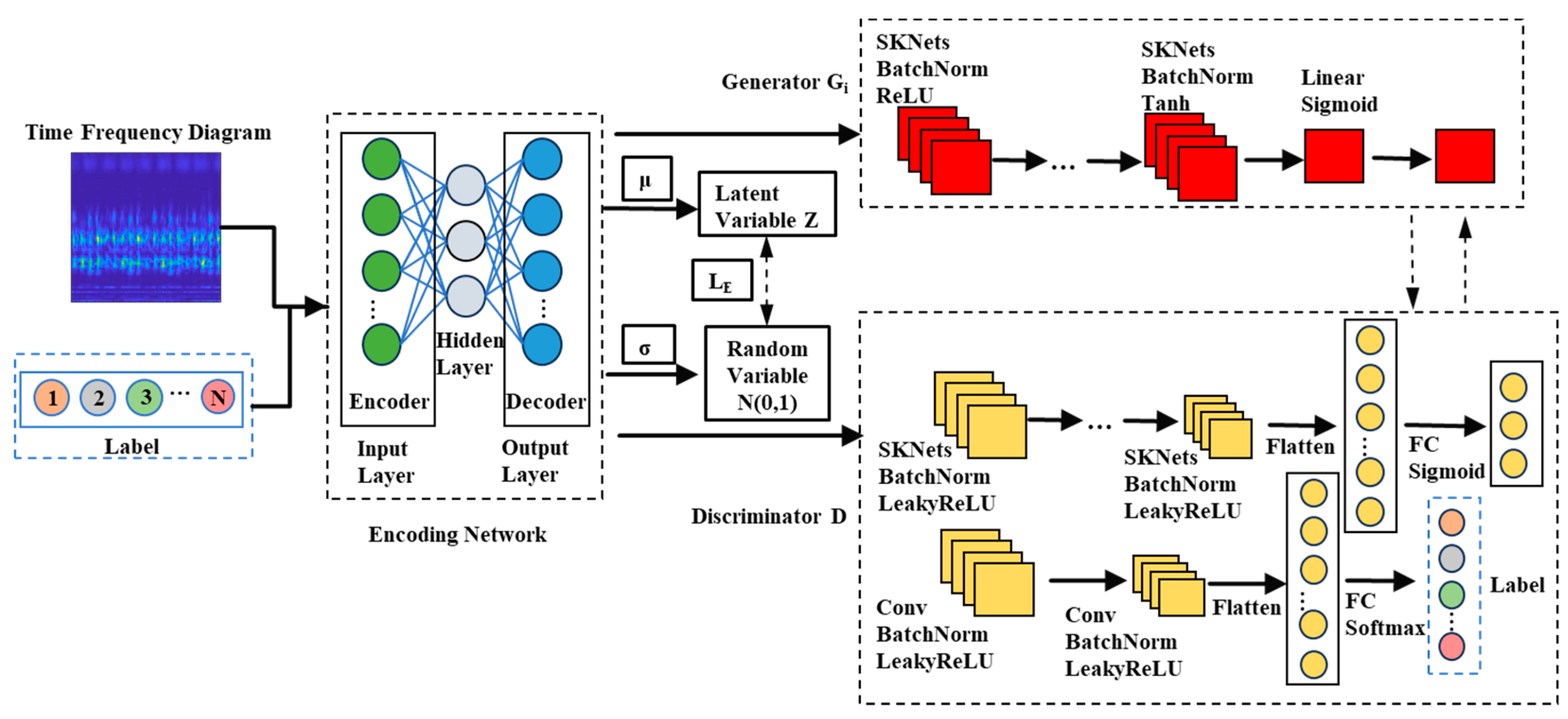
2.1. Architecture of CVAE-SKEGAN Network

In actual working conditions, machines operate in normal operations for most of the time, and fault samples are very scarce, resulting in sample imbalance problems. Time–frequency analysis methods have important application values in extracting transient features, conducting fault diagnosis, monitoring equipment status, etc., in mechanical systems. Time–frequency images can reveal rich information on bearing health status. Therefore, time–frequency images of bearing vibration signals are adopted as inputs to the network proposed for sample expansion operations, and pseudo time–frequency image samples are generated to expand fault samples. The structure of CVAE-SKEGAN network is shown in Figure 1, which is divided into three parts: encoding network, generator, and discriminator.

(1)

Encoding network

The encoding network consists of an encoder and a decoder. The encoder inputs 3-channel images, which are processed through convolutional layer, batch normalization, and LeakyReLU activation function. The output of the convolutional layer is flattened by a fully connected layer, and the mean and variance mapped to the latent space are output, respectively. Then, the latent variable Z is calculated via reparametrization. The decoder receives the latent variable Z and obtains a flattened output through a fully connected layer. The final 3-channel images are obtained through a convolutional layer, a batch normalization, and a ReLU activation function. CVAE-SKEGAN uses variational autoencoder (VAE), which is mainly used to reduce the dimensionality of raw data and model the underlying structure of the data. VAE compresses the input data into a low-dimensional latent space, converts each data point into a normal distribution, transforms high-dimentional data into concise latent vectors, and then decodes them back into an approximate representation of original data for next steps. The purpose is to improve the quality of the generated samples. The optimization objective of the encoding network is to minimize the K-L divergence between the noise distribution and the true image distribution, and its loss is calculated as shown in Equation (1).

$$L_E=KL\left(N\left(\mu ,{\sigma }^2\right)‖N\left(0,1\right)\right)={\displaystyle \frac{1}{2}}\left(-\log {\sigma }^2+{\mu }^2\right)$$

(1)

where $\mu$ is the mean mapped to the latent space, and ${\sigma }^2$ is the variance.

(2)

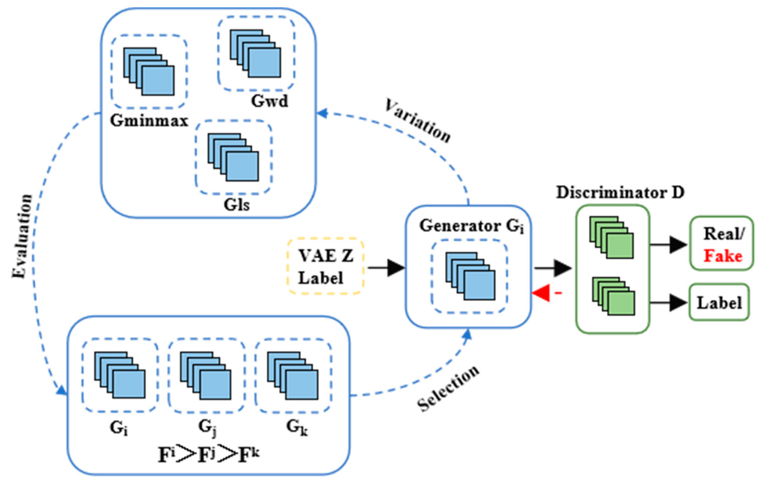
Generator

The input of the generator is images output by the encoding network. The optimization goal of the generator is to produce realistic samples to deceive the discriminator. The basic network of the generator consists of convolutional layers, linear layers, batch normalization, and activation functions. The convolutional layer incorporates SKNets [35] that enable the generator to adaptively select convolutional kernels during training and enhance the learning ability of the model. Due to the similarity of SKNets, one of the SK blocks is described. The specific structure of the SK block is shown in Figure 2. For kernel 3 × 3 and 5 × 5, element-wise summation operation is performed and inputs into GP layer. Finally, using the softmax layer, the output of the GP layer is computed to obtain a set of weights. These weights measure the features of different convolutional kernels to form the final output of the SK block.

To avoid the problem of gradient vanishing when using a single loss function, the genetic evolution structure in evolutionary generative adversarial networks (E-GAN) [36] is introduced to iteratively optimize through multiple loss functions. This enables the CVAE-SKEGAN model to select an adaptive generator for the next stage during the training process, thereby improving the quality and performance of the generator to adapt to the input data under different working conditions. The generator’s optimization process is shown in Figure 3. The specific process is as follows:

① Output images decoded by variational autoencoder (VAE) are fed into the generator G for mutation training using the minimax loss function, Wasserstein loss function, and LS loss function.

The minimax loss functions are shown in Equation (2).

$$\underset{G}{\min } \underset{D}{\max } L\left(G,D\right)=E_{x~P_{data}}\left[\log D\left(x\right)\right]+E_{z~P_z}\left[\log \left(1-D\left(G\left(z\right)\right)\right)\right]$$

(2)

where $x~P_{data}$ denotes x sampled from the true sample distribution $P_{data}$, $E\left(\ast \right)$ is the expected value, and $z~p_z\left(z\right)$ indicates the noise data z sampled from a standard normal distribution $p_z\left(z\right)=N\left(0,1\right)$.

The generator loss function of WGAN-GP is shown in Equation (3), and the discriminator loss function is shown in Equation (4).

$$\underset{G}{\min } L_G=-E_{G\left(z\right)~P_a}\left[D\left(G\left(z\right)\right)\right]$$

(3)

$$\underset{D}{\max } L_D=E_{x~P_{data}}\left[D\left(x\right)\right]-E_{G\left(z\right)~P_g}\left[D\left(G\left(z\right)\right)\right]-\lambda L_{GP}$$

(4)

where $G\left(z\right)~P_g$ represents that $G\left(z\right)$ is sampled from the generated sample distribution $P_g$, and λ is a tunable penalty parameter.

The gradient penalty term GP is shown in Equation (5).

$$\begin{array}{l}{L}_{GP}=E_{y~P_y\left(y\right)}\left[{\left({‖\nabla yD\left(y\right)‖}_2-1\right)}^2\right]\\ y=\gamma x+\left(1-\gamma \right)G\left(z\right)\end{array}$$

(5)

where y is a sample of random linear interpolation of x, $G\left(z\right)$$\gamma$ is a random coefficient, and $P_y$ indicates that the distributions of real and generated data are uniformly distributed along a straight line between pairs of sampling points.

The generator loss function using least squares loss is shown in Equation (6), and the discriminator loss function is shown in Equation (7).

$$L_G={\displaystyle \frac{1}{2}}{E}_{G\left(z\right)~P_g}\left[{\left(D\left(G\left(z\right)\right)-1\right)}^2\right]$$

(6)

$$L_D={\displaystyle \frac{1}{2}}{E}_{x~P_{data}}\left[{\left(D\left(X\right)-1\right)}^2\right]+{\displaystyle \frac{1}{2}}{E}_{G\left(z\right)~P_g}\left[{\left(D\left(G\left(z\right)\right)\right)}^2\right]$$

(7)

② The different mutations are evaluated, and the optimal solution is determined by using the fitness function F to score different loss functions. The fitness function F is divided into two parts: quality fitness function $F_q$ and diversity fitness function $F_d$.

The quality fitness score is the least squares fitness function.

$$F_q=E_z\left[{\left(D\left(z\right)-1\right)}^2\right]$$

(8)

The least squares fitness function is an unsaturated function, which means that the discriminator can promote generator optimization throughout the entire training phase, without allocating extremely high costs for generating fake samples. This can avoid gradient vanishing and pattern collapse.

The diversity fitness function $F_d$ measures the diversity of generated samples by utilizing the logarithmic gradient difference updated by the generator G and discriminator D.

$$F_d=-\log ‖{\nabla }_D‖+\log ‖{\nabla }_G‖$$

(9)

Thus, the final fitness function F is as follows:

$$F=F_q+\gamma F_d$$

(10)

where γ ≥ 0 balances two metrics.

③ The generator with a high adaptation score is used as the parent to move on to the next iteration until the network reaches the Nash equilibrium, and then the training ends.

The above process can avoid being limited to one single loss function, which is beneficial for alleviating the problem of gradient vanishing. The fitness function can effectively point to a suitable loss function. The evolutionary process can serve as a universal framework for different inputs, reducing the need to optimize the hyper-parameters for each individual dataset, thus making CVAE-SKEGAN applicable to multiple working conditions.

(3)

Discriminator

The inputs of the discriminator are the samples generated by the generator, the original real samples, and their corresponding label information. The discriminator is divided into two parts: true–false probability and classification discrimination. The input is a 28 × 28 × 1-dimensional feature sequence, which is processed in two parts: the true–false discrimination part simultaneously extracts features and reduces dimensions from generated samples and real samples to obtain a true–false probability output through Sigmoid activation function; after passing through two convolutional layers and flattening, the classification discrimination part obtains an output value of classification discrimination using Softmax activation function. In this function, the true–false discriminator part consists of convolutional structures and fully connected layers, and batch normalization operation is added after each convolutional layer. SKNets are also added to the true–false discrimination to improve the feature-extraction ability of the discriminator.

2.2. Assessment of Sample Generation Capability

In this study, a comparative experiment is conducted using the driving end data of the CWRU dataset, which contains different types of bearing faults, such as inner ring faults, outer ring faults, and rolling element faults, as well as bearing data under fault free conditions. The vibration data are collected at a sampling frequency of 12 KHz, and the faulty bearings are fabricated by electrical discharge machining. Each type of fault is distinguished by three different damage levels, so there are a total of 10 types of data. The data are converted into time–frequency images by Continuous Wavelet Transform (CWT) without pre-processing. A total of 100 time–frequency image samples are taken from each status type. The time–frequency images are generated using the WGAN-GP, CVAE-GAN, and CVAE-SKEGAN models, respectively. Maximum Mean Discrepancy (MMD) and Kullback-Leibler (K-L) divergence are used to evaluate the sample-generation capability and quality of the above three models.

(1)

MMD

MMD is used to evaluate whether the generated samples and the real samples conform the same probability distributions so as to reflect the sample generation ability. MMD mainly calculates the maximum average difference between the two distributions in the continuous function f. The larger MMD value, the more significant the difference between two distributions. Meanwhile, a smaller MMD value indicates that the difference in distributions is smaller, i.e., the distribution of the generated data is closer to that of the real data.

$$MMD\left[F,p,q\right]=\underset{f\in F}{\sup }\left(E_{x~p}\left[f\left(x\right)\right]-E_{y~q}\left[f\left(y\right)\right]\right)$$

(11)

where F denotes a set of continuous functions in the sample space, p and q denote two distributions, and x and y denote sample sets that satisfy the distributions p and q, respectively.

The MMD values are shown in

Table 1. MMD values for different models when generating different categories of data.

Fault Category	WGAN-GP	CVAE-GAN	CVAE-SKEGAN
0	1.342	2.562	0.431
1	1.277	2.353	0.277
2	1.407	2.570	0.407
3	1.291	2.191	0.291
4	1.358	2.506	0.358
5	1.395	2.379	0.395
6	1.403	2.334	0.403
7	1.271	2.251	0.271
8	1.444	2.504	0.444
9	1.315	2.451	0.315
Average	1.347	2.410	0.359

. It can be seen that the CVAE-SKEGAN model has a better sample-generation ability in model training.

(2)

K-L divergence

The K-L divergence can measure the information loss between two distributions. It is used to assess the generation loss of the generated data distribution compared to the real data distribution, thereby indicating the quality of the generated samples. The K-L divergence is calculated as follows:

$$KL\left(p‖q\right)={\displaystyle \sum _{i=1}^{n}p\left(x_i\right)\cdot \log \frac{p\left(x_i\right)}{q\left(x_i\right)}}$$

(12)

where p is the original distribution, and q is another distribution to approximate p.

As shown in

Table 2. K-L divergence values for different models when generating different categories of data.

Fault Category	WGAN-GP	CVAE-GAN	CVAE-SKEGAN
0	2.517	2.231	0.322
1	2.692	2.039	0.411
2	2.643	2.188	0.618
3	2.354	2.001	0.621
4	2.614	2.173	0.343
5	2.379	2.182	0.379
6	2.453	2.204	0.418
7	2.367	2.067	0.218
8	2.621	2.115	0.591
9	2.507	2.196	0.312
Average	2.515	2.140	0.423

, the CVAE-SKEGAN model can generate the best-quality samples.

MMD values and K-L divergence values of CVAE-SKEGAN are the smallest; the generated samples from this algorithm are the closest to the real sample distribution. The information loss of the generation process is minimal, and the generation ability is improved, indicating that the model improvement is effective. Therefore, CVAE-SKEGAN has an excellent performance in the sample-generation ability.

3. Bearing Fault Recognition Based on SSL-VCST Method

When there are insufficient training samples, deep learning-based fault diagnosis methods may not fully learn data features, which is not conducive to extracting fault features for classification or diagnosis. During the production process, it is difficult to obtain samples in fault states, and the cost of labeling fault samples is expensive. Most samples do not have status labels. This chapter addresses the issue of limited labeled samples by introducing SSL into a classification network. The network is trained by utilizing both labeled and unlabeled samples to extract fault features, avoiding the waste of unlabeled data and improving the accuracy of fault identification when there are insufficient samples.

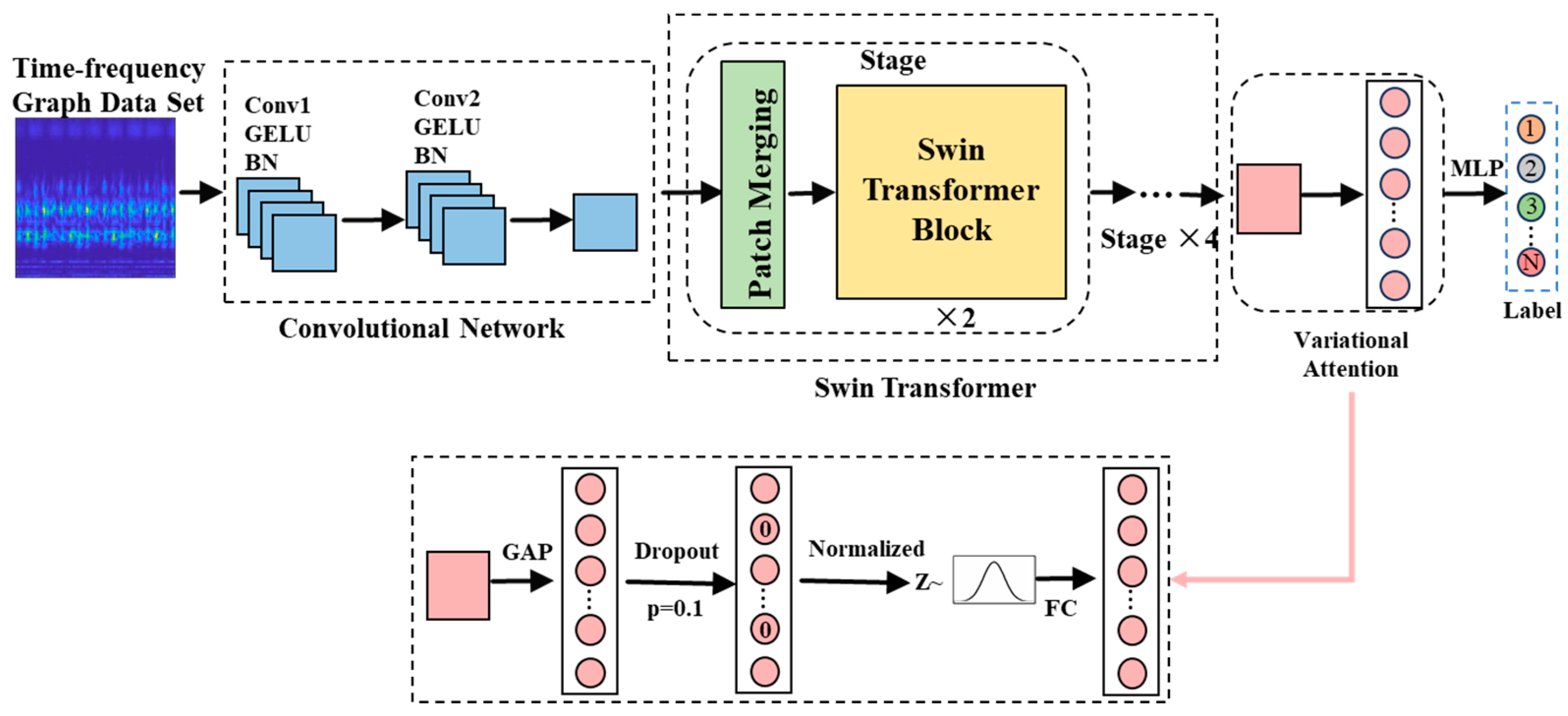
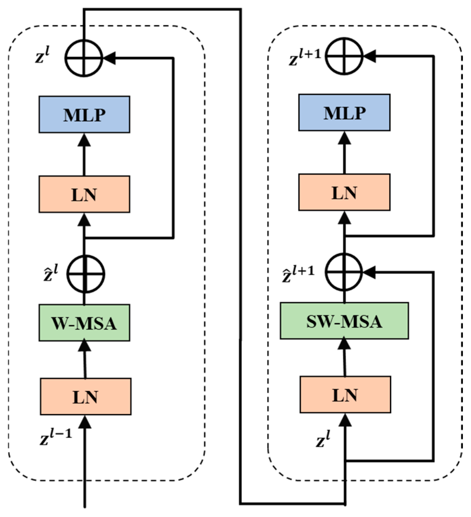
3.1. Architecture of VCST Network

Here, a basic classification network, VCST, is constructed by combining a CNN with a Swin Transformer (Swin-T) based on variational attention. The structure of the VCST network is shown in Figure 4.

The convolutional network module is used as a primary feature extractor to extract and integrate local features and global information from input images through convolutional layers, GELU activation functions, and batch normalization layers. Feature images output from the convolutional network module are input to Swin-T, and feature extraction and representation learning are carried out through four layers of Stage. Each Stage consists of a Patch Merging module and a Swin-T Block. The Patch Merging module is used to reduce dimensionality and reorganize image features. The Swin-T Block is responsible for multi-scale and multi-location abstraction as well as the encoding of image features. The structures of two consecutive Swin-T Blocks are shown in Figure 5. The first block consists of a Multilayer Perceptron (MLP), a Window Multihead Self-Attention Mechanism (W-MSA), and a Layer Normalization (LN) Block. The MLP is used for nonlinear transformations and mappings of input features, W-MSA is used to capture local and global feature relationships, and LN is used to normalize the outputs of each layer. The second module replaces the W-MSA in the first block with a Moving Window Multihead Self-Attention (SW-MSA), while the remaining parts remain unchanged.

W-MSA calculates self-attention separately by dividing an image into different windows. Feature maps are uniformly divided into small windows via window segmentation. Then, pixels are moved using a window configuration different from the previous layer’s window configuration. Residual computation is applied after each block, and successive Swin-T blocks are computed as follows:

$$\begin{array}{l}{\widehat{z}}^l=W-MSA\left(LN\left(z^{l-1}\right)\right)+z^{l-1}\\ z^l=MLP\left(LN\left({\widehat{z}}^l\right)\right)+{\widehat{z}}^l\\ {\widehat{z}}^{l+1}=SW-MSA\left(LN\left(z^l\right)\right)+z^l\\ z^{l+1}=MLP\left(LN\left({\widehat{z}}^{l+1}\right)\right)+{\widehat{z}}^{l+1}\end{array}$$

(13)

where $\widehat{z}$ denotes the (S)W-MSA output characteristics of block l, and $z^l$ denotes the MLP output characteristics of block l.

In the encoding process of Swin-T, let the length of input encoding be S and the dimension of single embedding space be D. The encoding can be represented as an S × D matrix. By multiplying by three weight matrices Wq, Wk, and Wv of size D × d, three coding matrices Q, K, and V of size S × d are obtained. The self-attention mechanism is calculated as follows:

$$Attention\left(Q,K,V\right)=soft\max \left({\displaystyle \frac{Q{K}^T}{\sqrt{d}}}+B\right)V$$

(14)

where d is the dimension of Q/K along each axis in the range of relative positions [−M + 1, M − 1] parameterizing a smaller size bias matrix $\widehat{B}\in R^{\left(2M-1\right)\times \left(2M-1\right)}$, and B is taken from $\widehat{B}$.

A variational attention mechanism is introduced after the attention matrix of Equation (14) to continue the computation. First, random zero padding is applied to the attention matrix using a dropout operation with a probability of 0.1, i.e., each element has a probability of 10% being zeroed during training. The masking of attention weights introduces randomness to reduce overfitting. Then, a normalization operation is performed on the attention matrix to ensure that the sum of attention weights is 1 so that it obeys a probability distribution. The specific calculation process is as follows:

$$\begin{array}{l}Att{n}_{dropout}^{\left(i\right)}=F_{.}dropout\left(Attentio{n}_i,p=0.1\right)\\ Att{n}_{normalized}^{\left(i\right)}={\displaystyle \frac{Att{n}_{dropout}^{\left(i\right)}}{{\displaystyle \sum _{i=0}^{n}Att{n}_{dropout}^{\left(i\right)}+\epsilon }}}\end{array}$$

(15)

where it is operated on the last dimension of attention—that is, calculate all the innermost elements of the tensor—and ε denotes the addition of a very small constant to avoid dividing by zero during the division operation and to ensure numerical stability.

The VCST network can fully utilize the advantages of CNN in local feature extraction as well as the transformer’s modeling ability in global correlations. Variational attention is used in the output computation of the attention matrix to provide more detailed information about attention weights and reduce the risk of overfitting so that it performs better and has better adaptability when training on diverse operating data.

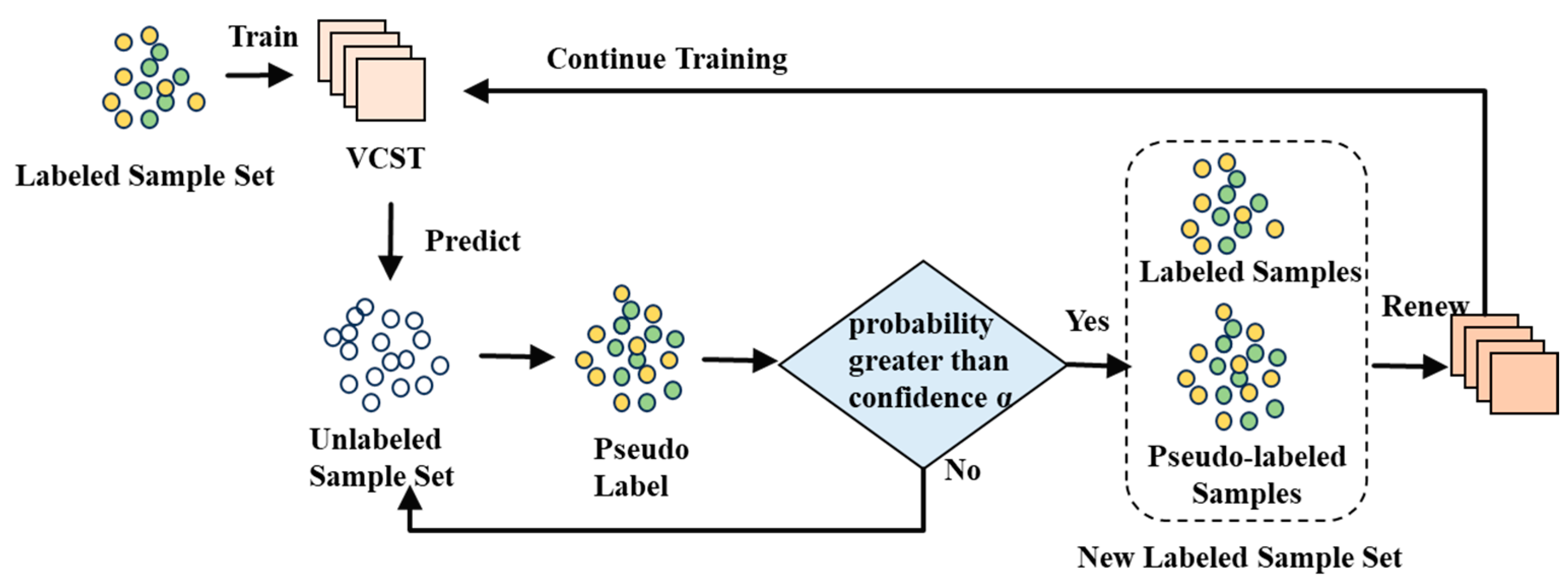
3.2. Principle of SSL-VCST Algorithm

To address the issue of insufficient labeled samples, SSL [37] is introduced into the VCST classification network utilizing unlabeled data for training. The core idea of SSL is to utilize unlabeled data by automatically generating labels to improve the generalization performance of the model. The cyclic training process of SSL-VCST is shown in Figure 6, and the specific training process is as follows:

(1) Supervised learning of labeled data. In the initial stage, supervised learning is performed on labeled data using a classification network. The maximum probability values after model prediction are used to optimize the network parameters by measuring the distance between prediction results and real labels through a cross-entropy loss function Equation (16). This ensures that the model has good performance on limited labeled data.

$$H\left(p,q\right)={\displaystyle \sum _{i=1}^L{p}_i\log \left(q_i\right)}$$

(16)

where $p_i$ is the true value, $q_i$ is the predicted value, and L is the category.

(2) Pseudo-label generation for unlabeled data. The trained model is applied to the unlabeled data, and if the probability value is greater than α (confidence level), its corresponding sample category is used as the pseudo-label value of the sample. Otherwise, the sample is considered temporarily unavailable. The confidence distribution is smoothed using Exponential Moving Average (EMA), as shown in Equation (17). For each new training round, an exponential moving average of the current confidence distribution is calculated and used as the dynamic threshold. This helps to reduce the fluctuation of the threshold and makes it more stable.

$$\alpha =\beta X_e+\left(1-\beta \right){\alpha }_{e-1}$$

(17)

where $\beta$ is the smoothing coefficient, and $X_e$ is the current training round value.

The interval of $\beta$ is (0, 1), which determines the contribution of new observations to the average value. In general, the closer to 1, the greater the impact of the new observations on the mean.

(3) Pseudo-labeled data fusion. The generated pseudo-labeled data are merged with labeled data to form an expanded dataset containing both of them.

(4) Recurrent training. The model is further trained on the merged dataset using consistent regularized loss, calculated as in Equation (18). It improves the model’s generalization ability for unknown data by predicting the same output on unlabeled data under different perturbations.

$$Loss=-{\displaystyle \frac{1}{N}}{\displaystyle \sum _{i=1}^{N}KL\left({\widehat{y}}_i^L‖{\widehat{y}}_i\right)}$$

(18)

where N is the number of consistent samples, ${\widehat{y}}_i^L$ is the pseudo-label, ${\widehat{y}}_i$ is the predicted probability of the model, and KL denotes the K-L divergence calculation.

(5) Until all data have been labeled, the expanded dataset completes the network training, and the diagnostic model is output to complete fault identification of the test set.

3.3. Assessment of Classification Ability with Insufficient Labeled Samples

Too inadequate of training samples can lead to limited learning of data distribution by deep learning models. Therefore, different sizes of training datasets are set to compare applicability and classification accuracy of Swin-T, VCST, and SSL-VCST networks based on a small sample. In all the classification experiments in this article, the training samples include real samples and generated samples. All real samples in the test sets and train sets come from different time periods of vibration signals based on the same batch of bearing and there is no overlap between test samples and train samples. All the original experimental data are labeled, and during the operation, a portion of the data is selected as labeled data to train the network, while a portion of the data is manually unlabeled to form unlabeled data. Considering the actual working environment where there is limited labeled data, GAN-generated samples are used to expand the labeled data. The experiments use the CWRU dataset with 10 types of data, and 4 sets of experiments are designed with labeled samples and unlabeled samples. Test sets evenly sampled from the 10 types of data, with the same-sized samples for each type of data. The total sample capacity of each task is shown in

Table 3. Experimental dataset settings.

Sample Size	T1	T2	T3	T4
Labeled samples	100	200	500	1000
Unlabeled samples	1000	1000	1000	1000
Test set	500	500	500	500

. Each experiment is run 10 times, and the average value is taken to avoid randomness. The training epoch is 100, and the learning rate is 0.001.

The SSL-VCST model can use unlabeled samples for auxiliary training of the network, and the rest of the models are trained using labeled samples. The average accuracy of different models under four task conditions is shown in Figure 7.

It can be seen that the accuracy of SSL-VCST is superior to other models in all four sets of tasks. In task T1, with the fewest labeled samples, the accuracy of Swin-T and VCST is lower than 0.9. However, the SSL-VCST model can reach 0.902. This indicates that even with a small size of labeled samples, SSL-VCST can still achieve high accuracy in the fault diagnosis of rolling bearings. With the gradual increase in labeled samples, the accuracy of each model improves, and SSL-VCST maintains the highest accuracy. In task T4, when the training samples are sufficient, the accuracy of each model exceeds 0.98, and the accuracy of SSL-VCST can reach 1. It can be proved that the SSL-VCST model can adapt to different sample situations and achieve a more stable accuracy with better generalization ability and stability.

4. Applicability Experiments on Imbalanced SAMPLES and Insufficient Labeled Samples under Multiple Operating Conditions

In the experimental-verification process in this section, the data-dividing method is consistent with Section 3.3.

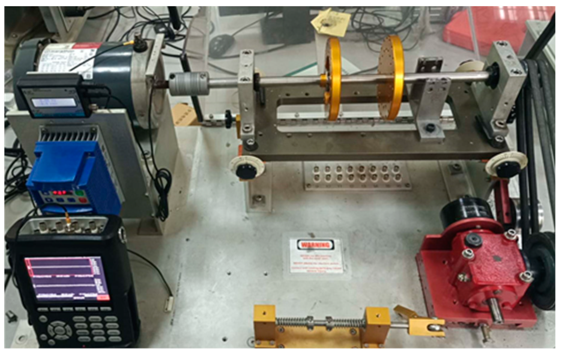
4.1. Experiment 1: Constant Speed Conditions of Rotating Machinery

Some scholars pointed out that among all bearing faults, outer ring failures and inner ring failures account for about 90%, and rolling element failures account for about 10% [38]. According to the above statistical data, the CWRU datasets are used for experimental setup, as shown in

Table 4. Experimental dataset setup under constant speed conditions.

Task	Sample Type	Normal	Inner Race Fault	Outer Race Fault	Ball Fault
T1	Training sets: Labeled samples	100	27	27	6
T2		100	45	45	10
T3		100	90	90	20
T1-T3	Training sets: Unlabeled samples	100	100	100	100
T1-T3	Testing sets	50	50	50	50

. First, CWT time–frequency images of all samples under four different states must be prepared. In actual operating conditions, the total number of labeled samples is relatively small, among which normal samples are the most abundant and easy to obtain. Therefore, the training sets include labeled samples and unlabeled samples, in which 100 normal samples are used for each of the three tasks, respectively. The samples for the other three fault states contain three different damage levels, and the sample quantity for each level is the same. In unlabeled samples, each state contains 100 samples, and the proportion of the three different damage levels is basically balanced. The testing sets are also set in the way, but the sample size is 50.

First, fault diagnosis is performed using CNN on the unbalanced sample sets as a basis for comparison. Then, after sample supplementation using the CVAE-SKEGAN method proposed in Section 2, a balance of 1:1:1:1 is achieved between normal and three fault samples. Fault diagnosis is carried out using SSL-VCST, SSL-CNN, and SSL-Swin-T to compare the fault diagnosis accuracy. SSL-CNN and SSL-Swin-T involve adding SSL mechanisms to both the CNN network and Swin-T network, respectively. The batch training size, learning rate, and optimization method are the same for all four models.

It can be known from Figure 8 that sample imbalance has a great impact on fault classification, and the more imbalanced the ratio between fault samples and normal samples, the worse the performance of fault classification. In the case of imbalanced data, using data generation for sample supplementation can improve classification accuracy. After balancing, the performance of the SSL-VCST model is clearly better than the other three methods. It can be proved that under constant rotational speed conditions of rotating machinery, the CVAE-SKEGAN method proposed for sample supplementation and the SSL-VCST model for fault diagnosis can better solve the problems of sample imbalance and labeled sample shortage.

4.2. Experiment 2: Variable Speed Conditions of Rotating Machinery

Experimental study of rotating machinery under variable speed conditions is conducted using the bearing datasets (SQV datasets) [39] publicly available from Xi’an Jiaotong University. The test rig is shown in Figure 9. The experimental data involve seven states, including normal state, inner ring failure, and outer ring failure, with three different damage levels, respectively. Each experiment process gradually accelerates from the stationary state to 3000 rpm and then gradually decelerates to 0 rpm. The sampling frequency is 25.6 KHz. Based on the SQV datasets, an unbalanced experiment is designed, and sample sizes are listed in

Table 5. Experimental dataset settings under variable speed conditions based on SQV datasets.

Task	Sample Type	Normal	Inner Race Fault	Outer Race Fault
T1	Training sets: Labeled samples	100	12	12
T2		100	27	27
T3		100	45	45
T1-T3	Training sets: Unlabeled samples	100	100	100
T1-T3	Testing sets	50	50	50

. The proportion for the three damage levels under each fault state is consistent with that under constant speed conditions.

Due to the time-varying nature of fault characteristic frequencies under variable speed conditions, the texture of CWT time–frequency images is prone to being indistinct, which limits the classification performance. Therefore, STFT time–frequency images are used as inputs instead. The sample supplementation and fault diagnosis operations are the same as those in Experiment 1. According to the comparison results shown in Figure 10, it can be seen that the accuracy of the SSL-VCST model is still the highest. It is verified that the proposed methods can still effectively solve the problems of sample imbalance and limited label samples under variable speed conditions of rotating machinery.

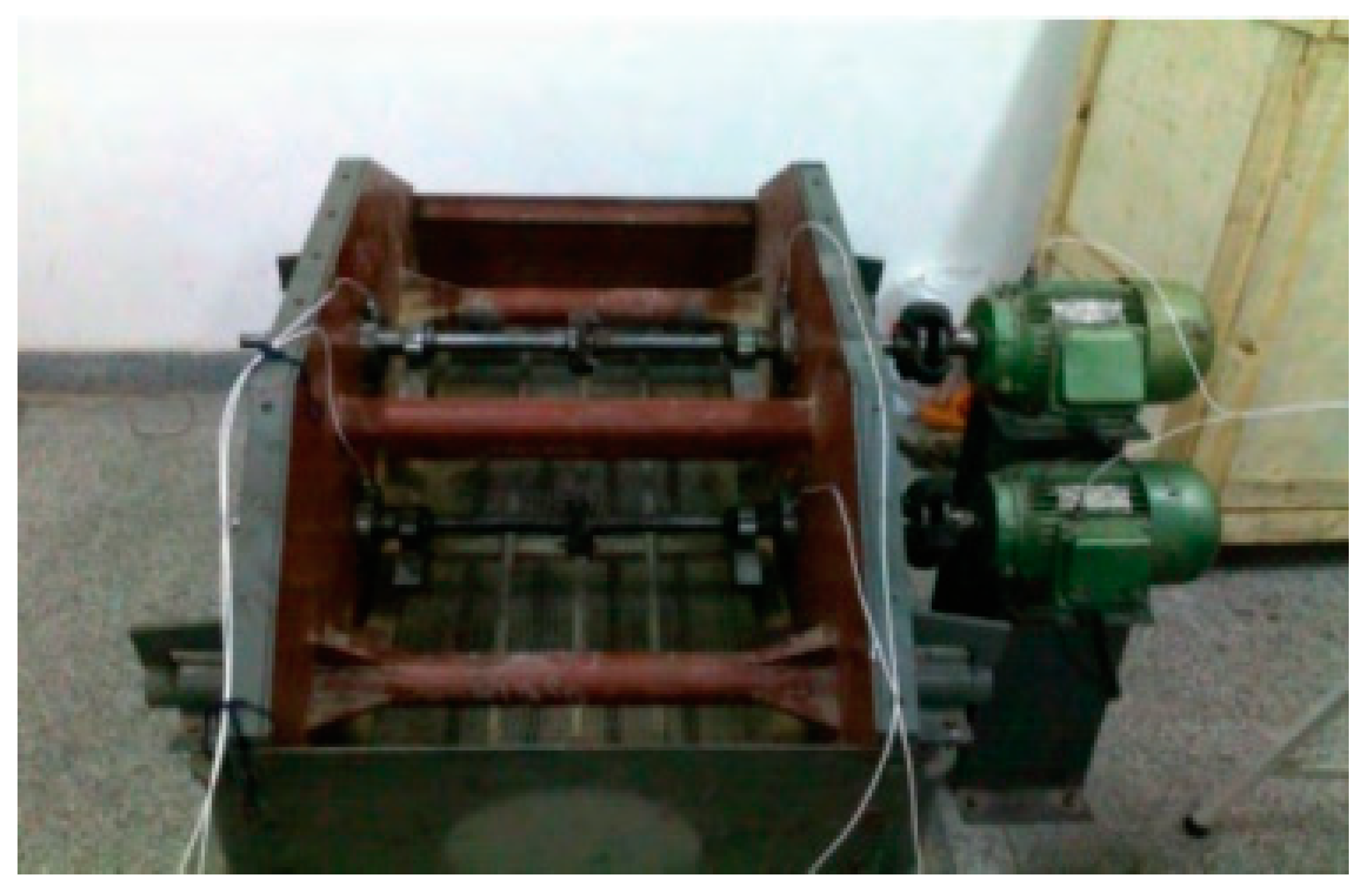
4.3. Experiment 3: Constant Speed Condition of Vibrating Machinery

In order to demonstrate the diversity of actual working conditions and verify the generalization ability of the proposed methods, the bearing datasets [40] of vibrating screens from Chang’an University are adopted. The test rig of the vibrating screen is shown in Figure 11. The datasets involve three types of bearing states, namely, the normal state, inner ring failure, and outer ring failure. The dataset design for the imbalanced sample experiment is similar to Experiment 1 and Experiment 2, which are detailed in

Table 6. Experimental dataset setup of vibrating screen under constant speed conditions.

Task	Sample Type	Normal	Inner Race Fault	Outer Race Fault
T1	Training sets: Labeled samples	100	12	12
T2		100	27	27
T3		100	45	45
T1-T3	Training sets: Unlabeled samples	100	100	100
T1-T3	Testing sets	50	50	50

.

It can be judged that even under strong noise interference conditions of vibrating machinery, the CVAE-SKEGAN model and SSL-VCST model still have high capabilities in capturing time–frequency image features of bearings in different states and fully utilizing unlabeled samples to guarantee fault diagnosis accuracy, as shown in Figure 12.

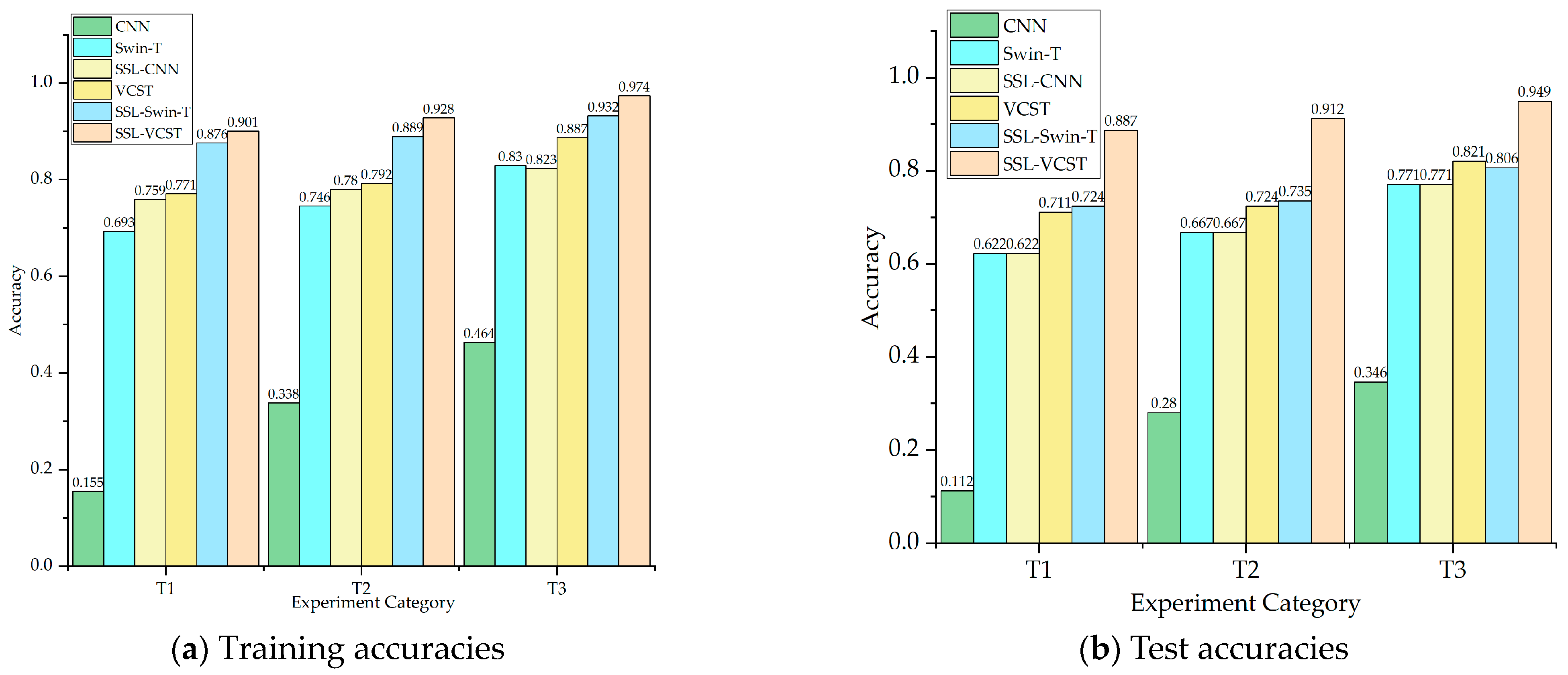
4.4. Experimental Analysis

From the above three experimental results, it can be seen that under the three operating conditions, the accuracies of the testing sets using CNN, Swin-T, and VCST decrease by an average of 0.07, 0.069, and 0.059, respectively, indicating that the variational attention mechanism can alleviate overfitting to a certain extent. In order to adapt to the situation of insufficient labeled samples, SSL is introduced to supplement training with unlabeled data. The accuracies of the testing set using SSL-CNN, SSL-Swin-T, and SSL-VCST decrease by an average of 0.088, 0.087, and 0.016, respectively. It can be seen that compared to the accuracies before the introduction of the SSL mechanism, the accuracies of the testing sets of SSL-CNN and SSL-Swin-T have further decreased slightly. It is considered that the process of assigning pseudo labels to unlabeled data by SSL depends on the training situation of the network itself, which affects the fitting effect in subsequent classification. However, SSL-VCST significantly improved the average accuracy compared to VCST, thus ensuring diagnostic accuracy. After comprehensively balancing variational attention and SSL mechanism, as well as considering the advantages of CNN and Swin-T, the SSL-VCST method proposed in this study has advantages in suppressing overfitting and improving fault diagnosis accuracy.

5. Conclusions

This study focuses on the practical problem of the low fault recognition of deep learning models due to the imbalance between normal and fault samples of rolling bearings, as well as insufficient labeled samples. A sample-expansion method based on GAN and a fault diagnosis method based on transformer were proposed, and the validity and applicability of the methods were confirmed by experimental data. The main conclusions are as follows:

(1)

To address the imbalance problem between normal and fault samples of bearings, a CVAE-SKEGAN network is proposed for the expansion of time–frequency image datasets. SKNets and genetic algorithms are introduced in CVAE-SKEGAN, which can adaptively select the convolutional kernel and the loss function to improve the model’s feature-learning ability and alleviate the problem of gradient vanishing. The experimental results show that the generated data distribution from CVAE-SKEGAN is closer to the real data distribution, and the information loss of the generated images is less.

(2)

Aiming at the challenge of inadequate labeled samples, an SSL-VCST network is proposed for bearing fault identification. In SSL-VCST, a variational attention mechanism is introduced to reduce the risk of overfitting and improve the adaptability of the model. The introduction of SSL fully utilizes unlabeled samples to supplement training, avoiding the waste of unlabeled data. The experimental results show that SSL-VCST can adapt to different sample imbalance levels and achieve a more stable accuracy. So, SSL-VCST has better generalization ability and stability.

(3)

The verification results under three typical operating conditions show that after the powerful balancing effect of the CVAE-SKEGAN, the SSL-VCST network is fully utilized to explore the value of unlabeled data, and the fault diagnosis accuracy achieved is significantly improved compared to other methods. The entire diagnostic scheme described here has strong applicability to multiple operating conditions.

Due to the high complexity and the high requirements for computing power of GAN, further research is needed to realize adaptive parameter tuning of the network to improve the efficiency of the training model. Of course, these issues cannot eliminate the proposed method from practical application. In addition, the data used for experimental validations come from experimental rigs, which still have a gap from the actual operation data. Further targeted adjustments are needed in subsequent research.

References

- Li, J.; Mao, W.; Yang, B.; Meng, Z.; Tong, K.; Yu, S. RUL prediction of rolling bearings across working conditions based on multi-scale convolutional parallel memory domain adaptation network. Reliab. Eng. Syst. Safe. 2024, 243, 109854. [Google Scholar] [CrossRef]
- Xu, F.; Ding, N.; Li, N.; Liu, L.; Hou, N.; Xu, N.; Guo, W.; Tian, L.; Xu, H.; Wu, C.L.; et al. A review of bearing failure Modes, mechanisms and causes. Eng. Fail. Anal. 2023, 152, 107518. [Google Scholar] [CrossRef]
- Henriquez, P.; Alonso, J.B.; Ferrer, M.A.; Travieso, C.M. Review of automatic fault diagnosis systems using audio and vibration signals. IEEE Trans. Syst. Man Cybern. Syst. 2013, 44, 642–652. [Google Scholar] [CrossRef]
- Zhu, Z.; Lei, Y.; Qi, G.; Chai, Y.; Mazur, N.; An, Y.; Huang, X. A review of the application of deep learning in intelligent fault diagnosis of rotating machinery. Measurement 2023, 206, 112346. [Google Scholar] [CrossRef]
- Zhang, S.; Zhang, S.; Wang, B.; Habetler, T.G. Deep learning algorithms for bearing fault diagnostics—A comprehensive review. IEEE Access 2020, 8, 29857–29881. [Google Scholar] [CrossRef]
- An, F.; Wang, J. Rolling bearing fault diagnosis algorithm using overlapping group sparse-deep complex convolutional neural network. Nonlinear Dynam. 2022, 108, 2353–2368. [Google Scholar] [CrossRef]
- Pham, M.T.; Kim, J.; Kim, C.H. Deep learning-based bearing fault diagnosis method for embedded systems. Sensors 2020, 20, 6886. [Google Scholar] [CrossRef]
- Janssens, O.; Slavkovikj, V.; Vervisch, B.; Stockman, K.; Loccufier, M.; Verstockt, S.; Van de Walle, R.; Van Hoecke, S. Convolutional neural network based fault detection for rotating machinery. J. Sound Vib. 2016, 377, 331–345. [Google Scholar] [CrossRef]
- Liu, T.; Zhang, C.; Lam, K.M.; Kong, J. Decouple and Resolve: Transformer-Based Models for Online Anomaly Detection From Weakly Labeled Videos. IEEE Trans. Inf. Forensics Secur. 2023, 18, 15–28. [Google Scholar] [CrossRef]
- Liu, Z.; Lin, Y.; Cao, Y.; Hu, H.; Wei, Y.; Zhang, Z.; Lin, S.; Guo, B. Swin Transformer: Hierarchical Vision Transformer using Shifted Windows. In Proceedings of the 2021 IEEE/CVF International Conference on Computer Vision (ICCV), Montreal, QC, Canada, 10–17 October 2021; IEEE: Piscataway, NJ, USA, 2021; pp. 9992–10002. [Google Scholar] [CrossRef]
- Huo, J.Y.; Li, C.J.; Yu, C.X. Multi-label industrial fault diagnosis method based on the Transformer network model. J. Vib. Shock 2023, 42, 189. [Google Scholar] [CrossRef]
- Yang, Z.; Cen, J.; Liu, X. Research on bearing fault diagnosis method based on transformer neural network. Meas. Sci. Technol. 2022, 33, 085111. [Google Scholar] [CrossRef]
- Jaber, M.M.; Ali, M.H.; Abd, S.K.; Jassim, M.M.; Alkhayyat, A.; Majid, M.S.; Alkhuwaylidee, A.R.; Alyousif, S. Resnet-based deep learning multilayer fault detection model-based fault diagnosis. Multimed. Tools Appl. 2024, 83, 19277–19300. [Google Scholar] [CrossRef]
- Qian, G.; Liu, J. A comparative study of deep learning-based fault diagnosis methods for rotating machines in nuclear power plants. Ann. Nucl. Energy 2022, 178, 109334. [Google Scholar] [CrossRef]
- Xu, K.; Kong, X.; Wang, Q.; Han, B.; Sun, L. Intelligent fault diagnosis of bearings under small samples: A mechanism-data fusion approach. Eng. Appl. Artif. Intel. 2023, 126, 107063. [Google Scholar] [CrossRef]
- He, Q.; Tang, X.H.; Li, C.J.; Lu, J.G.; Chen, J.D. Bearing fault diagnosis method based on small sample data under unbalanced loads. China Mech. Eng. 2021, 32, 1164–1171,1180. [Google Scholar] [CrossRef]
- Ma, R.; Han, T.; Lei, W. Cross-domain meta learning fault diagnosis based on multi-scale dilated convolution and adaptive relation module. Knowl.-Based Syst. 2023, 261, 110175. [Google Scholar] [CrossRef]
- Han, X.; Wang, Y.; Feng, J. A survey of transformer-based multimodal pre-trained modals. Neurocomputing 2023, 515, 89–106. [Google Scholar] [CrossRef]
- Jin, Y.; Hou, L.; Chen, Y. A Time Series Transformer based method for the rotating machinery fault diagnosis. Neurocomputing 2022, 494, 379–395. [Google Scholar] [CrossRef]
- Wang, G.; Liu, D.; Cui, L. Auto-embedding transformer for interpretable few-shot fault diagnosis of rolling bearings. IEEE Trans. Reliab. 2023, 73, 1270–1279. [Google Scholar] [CrossRef]
- Liu, S.; Chen, J.; He, S. Few-shot learning under domain shift: Attentional contrastive calibrated transformer of time series for fault diagnosis under sharp speed variation. Mech. Syst. Signal Proc. 2023, 189, 110071. [Google Scholar] [CrossRef]
- Goodfellow, I.J.; Pouget-Abadie, J.; Mirza, M.; Xu, B.; Warde-Farley, D.; Ozair, S.; Courville, A.; Bengio, Y. Generative adversarial nets. In Proceedings of the 27th International Conference on Neural Information Processing Systems, Montreal, QC, Canada, 8–13 December 2014; MIT Press: Cambridge, MA, USA, 2014; Volume 2, pp. 2672–2680. [Google Scholar] [CrossRef]
- Mirza, M.; Osindero, S. Conditional generative adversarial nets. arXiv 2014, arXiv:1411.1784. [Google Scholar]
- Zhang, Y.H.; Zhang, Z.Y.; Zhao, X.P.; Wang, L.H.; Shao, F.; Lu, K.Y. Bearing fault diagnosis method based on VAE-GAN and FLCNN unbalanced samples. J. Vib. Shock 2022, 41, 199–209. [Google Scholar] [CrossRef]
- Gulrajani, I.; Ahmed, F.; Arjovsky, M.; Dumoulin, V.; Courville, A. Improved training of wasserstein GANs. In Proceedings of the 31st International Conference on Neural Information Processing Systems, Long Beach, CA, USA, 4–9 December 2017; Curran Associates Inc.: Red Hook, NY, USA, 2017; pp. 5769–5779. [Google Scholar] [CrossRef]
- Mao, X.; Li, Q.; Xie, H.; Lau, R.; Wang, Z.; Smolley, S.P. On the effectiveness of least squares generative adversarial networks. IEEE Trans. Pattern Anal. Mach. Intell. 2018, 41, 2947–2960. [Google Scholar] [CrossRef] [PubMed]
- Liang, P.; Deng, C.; Wu, J.; Yang, Z.; Zhu, J.; Zhang, Z. Single and simultaneous fault diagnosis of gearbox via a semi-supervised and high-accuracy adversarial learning framework. Knowl.-Based Syst. 2020, 198, 105895. [Google Scholar] [CrossRef]
- Liu, J.; Zhang, C.; Jiang, X. Imbalanced fault diagnosis of rolling bearing using improved MsR-GAN and feature enhancement-driven CapsNet. Mech. Syst. Signal Process. 2022, 168, 108664. [Google Scholar] [CrossRef]
- Dixit, S.; Verma, N.K.; Ghosh, A.K. Intelligent fault diagnosis of rotary machines: Conditional auxiliary classifier GAN coupled with meta learning using limited data. IEEE Trans. Instrum. Meas. 2021, 70, 3517811. [Google Scholar] [CrossRef]
- Raouf, I.; Lee, H.; Kim, H.S. Mechanical fault detection based on machine learning for robotic RV reducer using electrical current signature analysis: A data-driven approach. J. Comput. Des. Eng. 2022, 9, 417–433. [Google Scholar] [CrossRef]
- Raouf, I.; Lee, H.; Noh, Y.R.; Youn, B.D.; Kim, H.S. Prognostic health management of the robotic strain wave gear reducer based on variable speed of operation: A data-driven via deep learning approach. J. Comput. Des. Eng. 2022, 9, 1775–1788. [Google Scholar] [CrossRef]
- Raouf, I.; Kumar, P.; Lee, H.; Kim, H.S. Transfer Learning-Based Intelligent Fault Detection Approach for the Industrial Robotic System. Mathematics 2023, 11, 945. [Google Scholar] [CrossRef]
- Raouf, I.; Kumar, P.; Cheon, Y.; Tanveer, M.; Jo, S.H. Advances in Prognostics and Health Management for Aircraft Landing Gear—Progress, Challenges, and Future Possibilities. Int. J. Precis. Eng. Manuf.-Green Tech. 2024. [Google Scholar] [CrossRef]
- Kumar, P.; Raouf, I.; Kim, H.S. Transfer learning for servomotor bearing fault detection in the industrial robot. Adv. Eng. Softw. 2024, 194, 103672. [Google Scholar] [CrossRef]
- Li, X.; Wang, W.; Hu, X.; Yang, J. Selective Kernel Networks. In Proceedings of the 2019 IEEE/CVF Conference on Computer Vision and Pattern Recognition (CVPR), Long Beach, CA, USA, 15–20 June 2019; IEEE: Piscataway, NJ, USA, 2019; pp. 510–519. [Google Scholar] [CrossRef]
- Wang, C.; Xu, C.; Yao, X.; Tao, D. Evolutionary generative adversarial networks. IEEE Trans. Evol. Comput. 2019, 23, 921–934. [Google Scholar] [CrossRef]
- Shahshahani, B.M.; Landgrebe, D.A. The effect of unlabeled samples in reducing the small sample size problem and mitigating the Hughes phenomenon. IEEE Trans. Geosci. Remote Sens. 1994, 32, 1087–1095. [Google Scholar] [CrossRef]
- Bently, D. Predictive maintenance through the monitoring and diagnostics of rolling element bearings. Bently Nev. Co. Appl. Note 1989, 44, 2–8. [Google Scholar]
- Liu, S.; Chen, J.; He, S.; Shi, Z.; Zhou, Z. Subspace network with shared representation learning for intelligent fault diagnosis of machine under speed transient conditions with few samples. ISA Trans. 2022, 128, 531–544. [Google Scholar] [CrossRef]
- Xu, Y.B.; Cai, Z.Y.; Hu, Y.B.; Ding, K. A frequency-weighted energy operator and variational mode decomposition for bearing fault detection. J. Vib. Eng. 2018, 31, 513–522. [Google Scholar] [CrossRef]