Multi-Layer Objective Model and Progressive Optimization Mechanism for Multi-Satellite Imaging Mission Planning in Large-Scale Target Scenarios

Abstract

With the continuous increase in the number of in-orbit satellites and the explosive growth in the demand for observation targets, satellite resource allocation and mission scheduling are faced with the problems of declining benefits and stagnant algorithm performance. This work proposes a progressive optimization mechanism and population size adaptive strategy for an improved differential evolution algorithm (POM-PSASIDEA) in large-scale multi-satellite imaging mission planning to address the above challenges. (1) MSIMPLTS based on Multi-layer Objective Optimization is constructed, and the MSIMPLTS is processed hierarchically by setting up three sub-models (superstructure, mesostructure, and understructure) to achieve a diversity of resource selection and step-by-step refinement of optimization objectives to improve the task benefits. (2) Construct the progressive optimization mechanism, which contains the allocation optimization, time window optimization, and global optimization phases, to reduce task conflicts through the progressive decision-making of the task planning scheme in stages. (3) A population size adaptive strategy for an improved differential evolution algorithm is proposed to dynamically adjust the population size according to the evolution of the population to avoid the algorithm falling into the local optimum. The experimental results show that POM-PSASIDEA has outstanding advantages over other algorithms, such as high task benefits and a high task allocation rate when solved in a shorter time.

1. Introduction

Multi-satellite Imaging Mission Planning (MSIMP) refers to the priority scheduling of high-priority tasks to maximize the number of task completions and mission benefits in a complex environment by efficiently allocating limited satellite resources within a limited time window to meet the diversified image requirements of multi-source users [1,2]. At present, it has been widely used in many fields, such as disaster emergency response and assessment [3], urban infrastructure monitoring [4], climate change and environmental protection assessment [5], etc. However, with the increasing number of satellites in orbit and the gradual expansion of application scenarios, the demand for observation targets has shown exponential growth. In recent years, the demand for image data in disaster emergency response has increased by more than 20% in recent years [6], placing higher demands on mission response timeliness, mission benefits, and mission completion. To be specific, response timeliness requires rapid access to image data during emergencies, task gain requires more efficient resource utilization through optimized task scheduling, and task completion requires that all planned tasks are completed as far as possible to meet the needs of different priorities.

In MSIMP on a regular scale (more than tens of targets), there are difficulties such as a long response time, low mission benefit, and low mission execution rate due to multiple factors, such as limited satellite resources, spatial and temporal inhomogeneity of orbit coverage, and restricted time window for observation tasks. Taking disaster emergency response as an example, flooding in a certain region requires that high-resolution satellite images be acquired within three hours for rescue deployment; however, due to the time window of satellite orbit coverage and other tasks, the satellite fails to acquire key images in time, making the delayed images lose their actual decision-making value. At the same time, the observation requirements for multiple tasks in the region resulted in some low-priority tasks not being able to be performed or insufficiently observed, reducing the task execution rate [7,8]. These problems are particularly acute in large-scale target mission scenarios. The simultaneous demand for hundreds of observation targets exacerbates satellite resource conflicts and competition for time windows, leading to an exponential increase in the complexity of mission planning. In a global climate monitoring mission, multiple countries simultaneously demand satellite observation images of different regions, and 300 targets must be observed globally within 24 h, while the execution priorities and time windows of the targets are different, which greatly increases the response time of the MSIMP system, and in addition, the limitations of the number of satellites and orbital coverage may delay some of the low-priority tasks, which has an impact on the mission benefit mission revenue and mission completion [9].

Multi-satellite imaging mission planning in large-scale target scenarios (MSIMPLTS) aims to optimize satellite resource allocation and mission scheduling through a systematic approach, which improves the mission response speed, increases the mission execution rate, and maximizes the mission benefit to cope with the complexity of large-scale target missions. MSIMPLTS can practically solve the key challenges in mission planning by improving the optimization algorithms and dynamic scheduling strategies: firstly, MSIMPLTS can quickly match satellite resources and mission requirements to significantly shorten the response time; secondly, MSIMPLTS can reduce resource conflicts and scheduling bottlenecks by reasonably allocating mission priorities and time windows and improve the mission response time; secondly, it can reduce the resource conflicts and scheduling bottlenecks by reasonably allocating mission priorities and time windows and improve the mission response time by reasonably allocating satellite resources and mission requirements. In addition, MSIMPLTS can use an intelligent scheduling strategy to adjust satellite resource allocation in real time to enhance system adaptability in the face of large-scale target mission environments. Therefore, the investigation of MSIMPLTS provides a new solution to the practical difficulties in large-scale mission planning and is of great significance in solving the conflict between limited satellite resources and the explosive growth of target observation demand.

In actual applications, remote sensing technology has been widely used to provide strong support for mission scheduling and emergency response in complex scenarios. A large amount of the literature has shown that remote sensing data have important roles in areas such as disaster emergency response, urban infrastructure monitoring, and climate change assessment. For example, using satellite rainfall products to evaluate the impacts of natural disasters [10], using General Circulation Models (GCMs) to quantify climate change [11], and investigating the impacts of manmade infrastructures on river morphology under global warming, as well as applications in environmental protection [12] and disaster emergency response [13], have fully demonstrated the great potential of satellite imaging technology. Particularly in enhancing human resilience in coastal communities [14], these applications further demonstrate the critical role of satellite imaging technology in addressing global environmental and disaster challenges. Therefore, in-depth research on MSIMPLTS will provide new ways to solve these practical problems and promote mission planning for efficient and intelligent scheduling in a wider range of application scenarios.

Presently, MSIMPLTS can be classified into two parts: task planning models and task planning algorithms, according to the type of target task, constraints of task planning, and scale of planning scenarios.

Research on MSIMPLTS task planning models includes the integer planning model [15], constraint satisfaction model [16], agent model [17], graph theory model [18], Markov decision model [19], Graph Neural Network (GNN) model [20], etc. Lorena Linares et al. [21] further applied the Mixed Integer Linear Programming (MILP) model to solve the computational efficiency problem of task assignment in large-scale scenarios. Yang et al. [22] proposed an intelligent task-solving framework based on the constraint satisfaction model, which realized the autonomous adjustment of the observation sequence of the target task in large-scale scenarios. Li et al. [23] combined the description methods of attributes, interactions, rules, and states through agent technology to solve the complexity problem of multi-satellite resource allocation and coordination. Wang et al. [24] proposed a graph theoretical model for the automatic aggregation of MSIMPLTS problems, modeling MSIMPLTS problems as heterogeneous graphs following various constraints, which effectively improves large-scale target scenario mission planning in terms of task benefits. He et al. [25] modeled the MSIMPLTS problem as a finite Markov decision process with a continuous state space and a discrete action space, which solved the task planning problem under uncertainty and diverse demands. Zhibo [26] proposed a graph neural network model based on MSIMPLTS, which improves the speed of reaching the optimal task planning solution for large-scale scenarios.

Research on algorithms for MSIMPLTS task planning includes the greedy algorithm [27], mixed integer programming algorithm [28], local search algorithm [29], intelligent optimization algorithms [30], heuristic algorithms [31], and deep learning methods [32]. Chang et al. [33] proposed a greedy algorithm considering both observation task priority and task congestion, which improves the image duration of observation tasks in large-scale scenarios. Ayana et al. [34] proposed a mixed-integer programming algorithm to solve MSIMPLTS by maximizing the objective function, considering factors such as satellite resource consumption and user request priority in large-scale scenarios. Chen et al. [35] proposed a local search algorithm to solve the target task planning problem in large-scale scenarios, and its efficient constraint handling mechanism improves the algorithm’s efficiency. Wang et al. [36] utilized the overall benefits of an optimized task, antenna load balancing, and task completion timelines simultaneously and proposed a multi-objective differential evolutionary algorithm based on spatial partitioning and an adaptive selection strategy to solve the difficult problem of inefficient allocation in large-scale scenarios. He et al. [37] proposed heuristic algorithms based on an edge computing framework to ensure that satellite missions in large-scale scenarios can be optimized in terms of resource utilization. Chen’s [38] deep reinforcement learning procedure trained encoder–decoder-structured neural networks (NNs) to achieve simultaneous optimization of the failure rate and response time of a multi-satellite imaging mission planning system in large-scale scenarios.

Most of the models and algorithms proposed in the current research belong to the holistic optimization approach, which significantly improves the planning ability; however, it also brings about an increase in the computational complexity and an extension of the planning time. In addition, allocation conflicts among multiple tasks make the optimal allocation of resources difficult to achieve. The specific difficulties are as follows:

• Addressing the MSIMPLTS problem requires considering multiple optimization objectives, such as the target task benefit, task allocation rate, and response time. Most of the current studies use single-objective optimization models to achieve the optimal solution by setting the weights of different objectives. However, conflict or mutual constraints between the optimization objectives make it difficult to obtain high-quality task-planning solutions. In this context, designing optimization models that can take into account the interactions and constraints between the objectives is a new challenge in solving the MSIMPLTS problem.
• Existing research on the MSIMPLTS problem mainly focuses on the study of the sequence of satellite-target mission assignments, ignoring the feature that the same satellite resource can observe multiple targets at the same time. This leads to difficulties such as overlapping observation time windows, conflicting planning programs, and low utilization of satellite resources. Therefore, constructing a more reasonable mission planning method is a major objective for MSIMPLTS work.
• Large-scale target task requirements lead to a significant increase in the problem decision dimension and a larger solution space. The current MSIMPLTS-solving algorithms mostly focus on improving the ratio of feasible solutions, which leads to problems such as the mission planning scheme easily falling into local optimums or converging prematurely. Going forward, designing reasonable solution algorithms that effectively balance the solution efficiency and solution quality is also another challenge for MSIMPLTS studies.

To overcome these difficulties, this work takes imaging satellites as the research object and proposes a progressive optimization mechanism and population size adaptive strategy for an improved differential evolution algorithm in large-scale target scenarios. The main contributions of this work are as follows:

• In terms of constructing a task planning model, we propose the MSIMPLTS based on Multi-layer Objective Optimization (MSIMPLTS-MLOO). The model is structured by setting up three layers: the superstructure, mesostructure, and understructure, with each layer focusing on a different optimization objective. These, respectively, optimize the task benefit, task completion, and response time functions. At each level, a resource selection diversity approach is used, which helps to better balance the interactions and constraints between the optimization objectives.
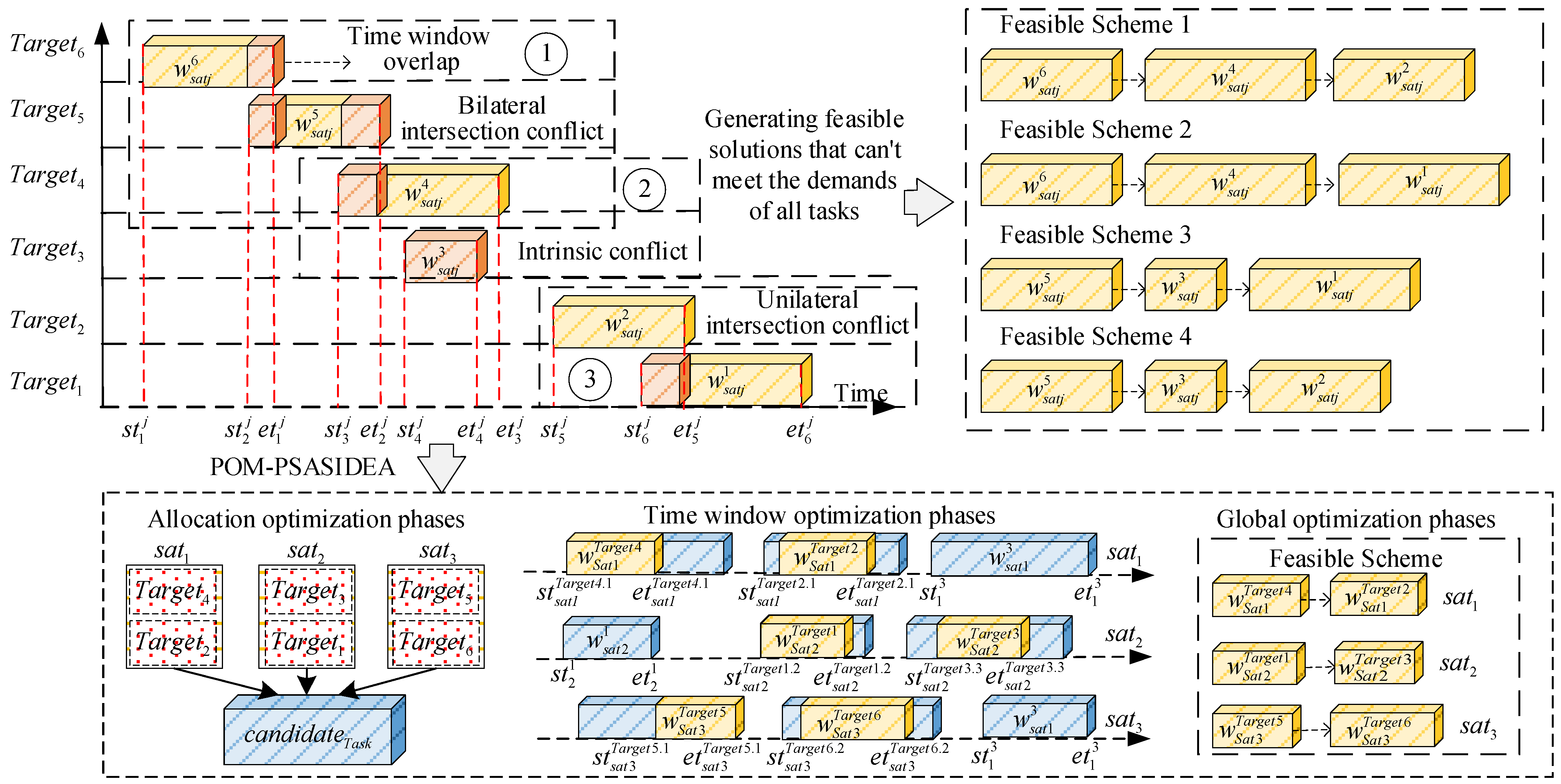
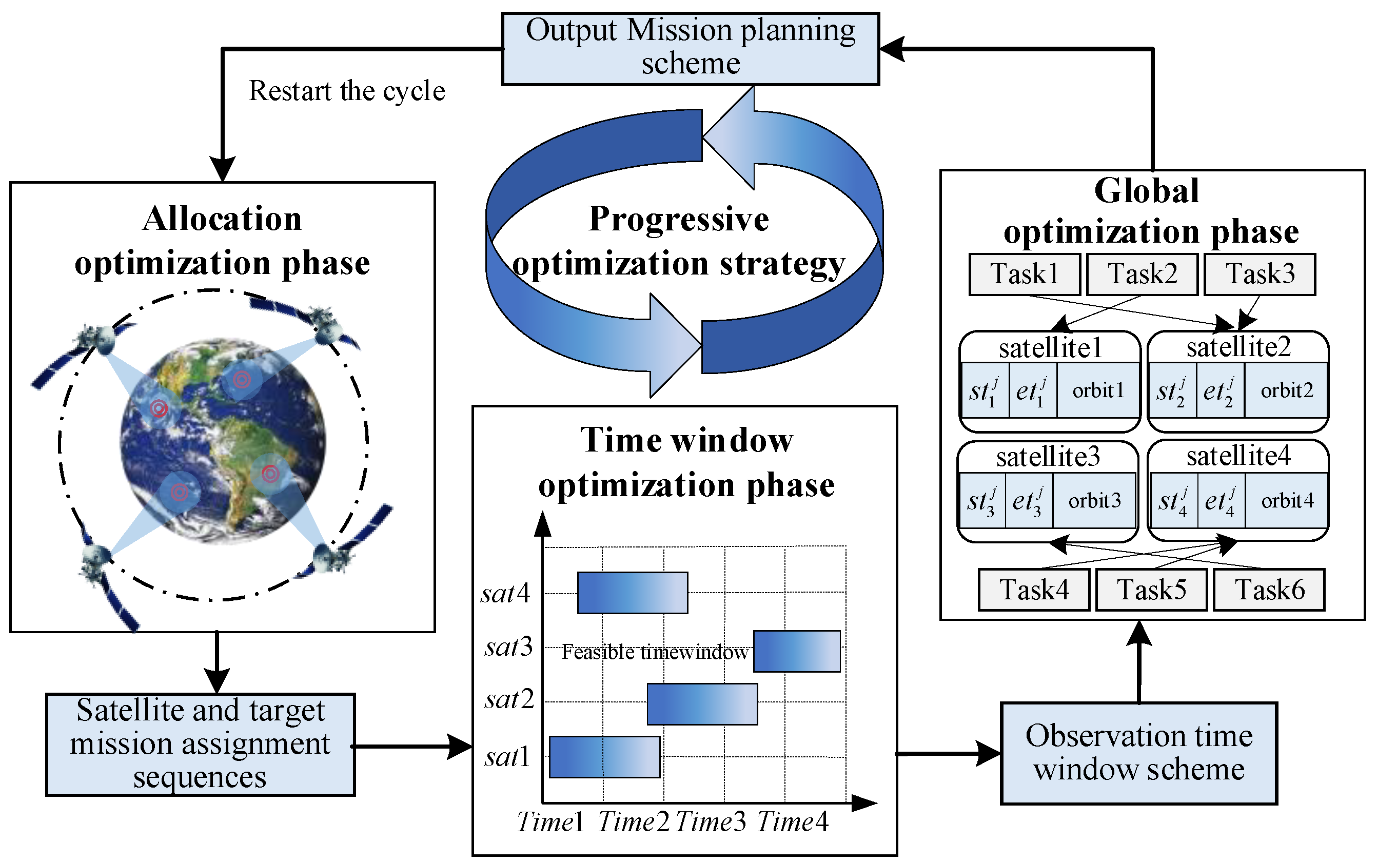
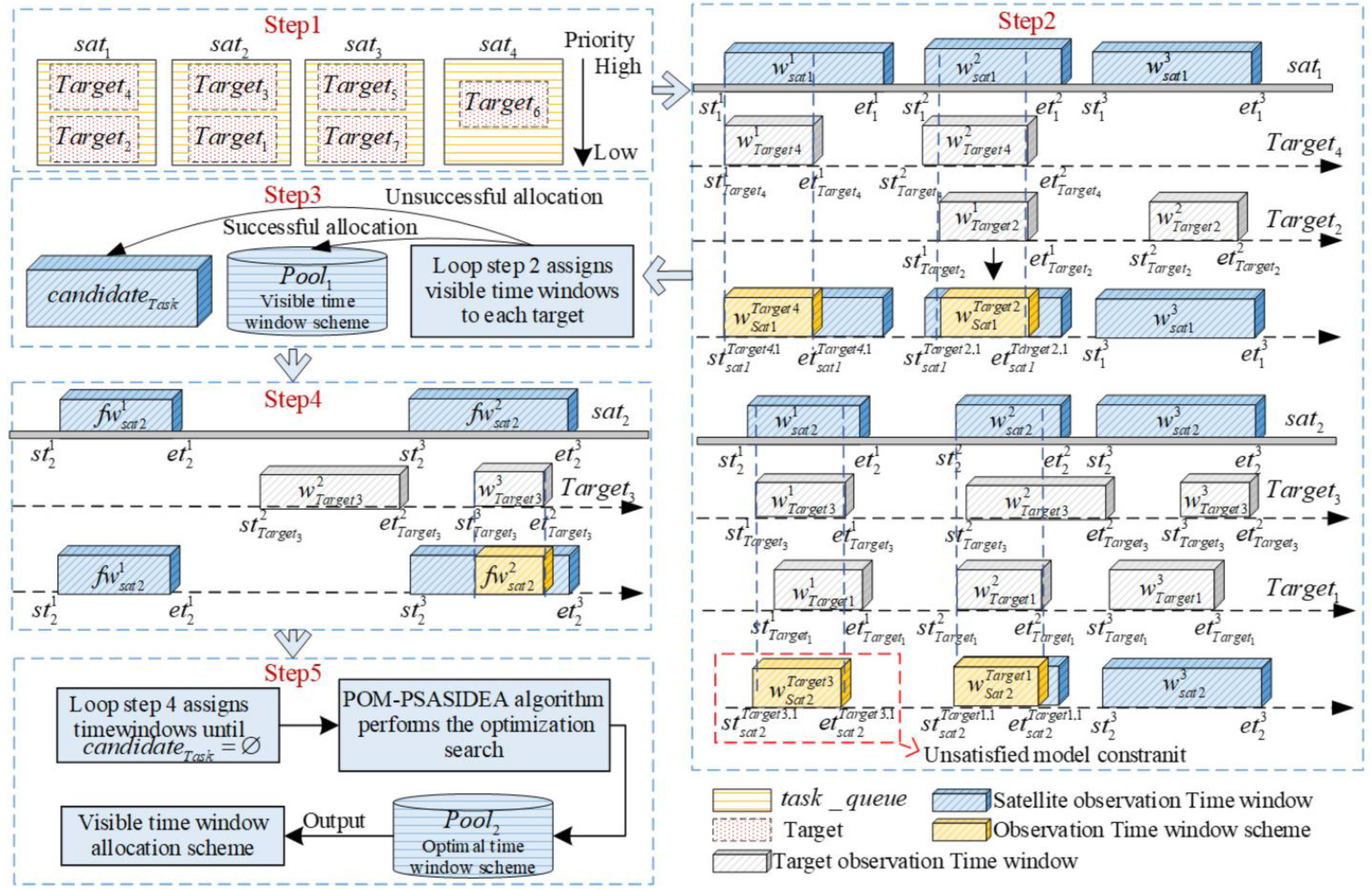
• In terms of the mission planning methodology, we propose a progressive optimization mechanism. Firstly, an initial task planning scheme is generated in the allocation optimization phase, which contains the allocation sequences of satellites and target tasks. Secondly, in the time window optimization phase, an execution time window is assigned to each target task based on the planning scheme in the allocation optimization phase. Finally, the planning results of the previous two phases are combined in the global optimization phase to generate the final mission planning scheme. Through stage-by-stage incremental decision-making, conflicts between planning schemes can be reduced, and the utilization rate of satellite resources can be effectively improved.
• In terms of constructing the mission planning algorithm, a population size adaptive strategy for an improved differential evolution algorithm is proposed to address the problem that multiple satellites are prone to falling into the local optimal solution under the large-scale target mission scenario, as well as for solving the difficulty of different constraints faced by the three-layer structure of the MSIMPLTS-MLOO model. The algorithm dynamically adjusts the population size according to the evolution of the population to adapt to the needs for model solving and thus improve the solving efficiency and quality of the mission planning scheme.

The rest of the work is organized as follows: Section 2 introduces the basic MSDMP scenario and the motivation for studying MSIMPLTS. Section 3 introduces the MSIMPLTS model and its objective function and constraints. Section 4 details the specifics of the POM-PSASIDEA algorithm. Section 5 presents our simulation experiments to analyze the effectiveness and stability of the POM-PSASIDEA algorithm. Section 6 concludes and offers future perspectives.

2. Related Works

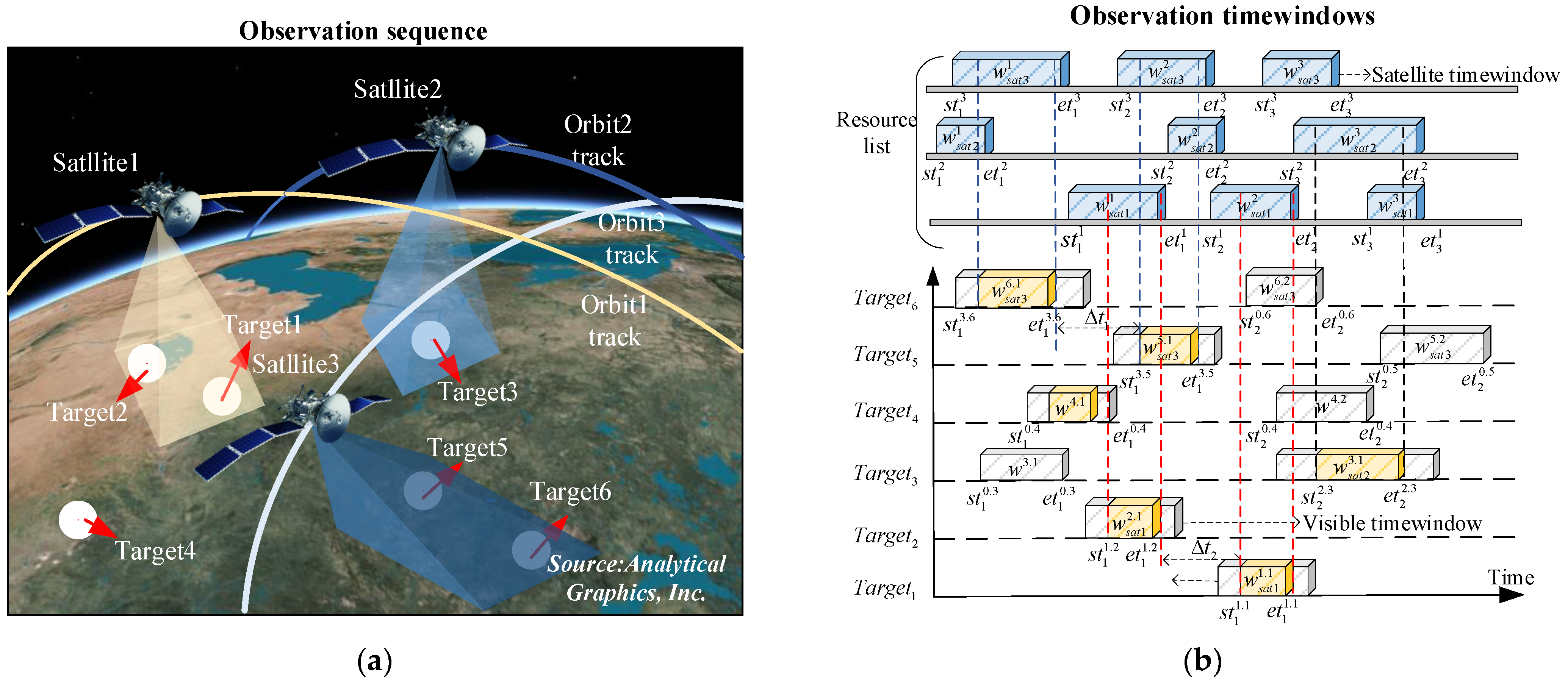
2.1. MSIMP Basic Mission Scenarios

MSIMP aims to coordinate multiple satellites for efficient imaging of target areas by optimizing satellite resources and time allocation. Firstly, the mission requirements and satellite resources of MSIMP are analyzed to determine the satellites to be observed and the mission information. It is assumed that $N_{Target}$ observation mission $\left\{Targe{t}_i\right|i=1,\dots 6\}$ is performed by a set of satellites $\left\{sa{t}_j\right|j=1,\dots 3\}$ at a certain regional scale, with a satellite executable orbit of $\left\{Orbi{t}_k|k=1,\dots ,3\right\}$. Each observation mission has multiple visible time windows $w=\left\{w_{satj}^{i,g}|j\in sat,i\in Target,g\in window\right\}$ with multiple satellite resources, and each satellite resource is capable of performing multiple observation missions. Secondly, a mission planning solution algorithm is used to obtain the optimal MSIMP mission planning scenario within the mission planning time $[pla{n}_{start},pla{n}_{end}]$. This includes the assignment sequence and the visible time window planning scenario. The basic MSIMP mission scenario is shown in Figure 1.

Figure 1a shows the sequence of multi-satellite imaging mission assignments, specifically $(Sa{t}_1,Targe{t}_1,Targe{t}_2)$, $(Sa{t}_2,Targe{t}_3)$, and $(Sa{t}_3,Targe{t}_5,Targe{t}_6)$. Figure 1b shows the visible time window allocation scheme for each satellite and the target task, in which the blue rectangle represents the visible time window for the satellite, the gray rectangle represents the visible time window for the observation task, and the yellow rectangle represents the observation time window for the satellite to the target task. The specific time window allocation is $(Targe{t}_1,[s{t}_1^{1,1},e{t}_1^{1,1}])$, $(Targe{t}_2,[s{t}_1^{1,2},e{t}_1^{1,2}])$, $(Targe{t}_3,[s{t}_2^{2,3},e{t}_2^{2,3}])$, $(Targe{t}_5,[s{t}_1^{3,5},e{t}_1^{3,5}])$, and $(Targe{t}_6,[s{t}_1^{3,6},e{t}_1^{3,6}])$, where $s{t}_g^{j,i}$ and $e{t}_g^{j,i}$ represent the start and end times of observation mission $i$ in the $g$-th time window on satellite $j$, respectively. Finally, the satellite performs corresponding assigned tasks according to the mission planning scheme, further evaluates the implementation effects of the tasks, and makes corresponding adjustments to the follow-up mission scheme according to the evaluation results [39,40].

2.2. Motivation

The fundamental ideology of the existing research on the MSIMPLTS problem is to decompose the large-scale problem into multiple smaller sub-problems for solving from the spatial dimension, i.e., divide the objective task into multiple subsets based on the decision vector of the search space and optimize multiple objective functions simultaneously according to the characteristics of the global search to achieve a reduction in the objective space in the scenario of large-scale objective tasks [20,41]. The global optimization of the MSIMPLTS planning scheme relies solely on the optimization algorithm, ignoring the correlation between satellite performance conditions and target tasks. Figure 2 shows a schematic diagram of observation time window conflicts in the mission planning scheme under the classical global optimization method, including three types of satellite observation time window conflicts for multiple target missions: unilateral intersection, bilateral intersection, and intrinsic conflicts.

It can be seen that the observation time windows overlap highly in the mission planning cycle, and the combined characteristics of the MSIMPLTS problems can be seen more clearly. The MSIMPLTS scheme faces several challenging issues, including overlapping observation time windows, abnormal target task allocation, satellite resource conflicts, and poor task execution timeliness. These factors make it difficult to obtain high-quality planning schemes within a limited time. This motivated us to build the MSIMPLTS model based on multi-layer optimization and a progressive optimization mechanism.

To address the aforementioned issues, a research approach based on the MSIMPLTS model based on multi-layer optimization and the progressive optimization mechanism is proposed. The different optimization objectives at various layers of this model can complement each other, reducing the risk of potential solution loss and enhancing the globality and diversity of the solutions. At the same time, the progressive optimization mechanism refines and adjusts the optimization process step by step, more effectively balancing the efficiency and quality of the solution. By employing staged optimization (including task allocation, time window optimization, and global optimization phases), the process gradually approaches the optimal solution, overcoming the limitations of a single-layer global optimization method, ultimately solving the multi-satellite imaging mission planning problem in large-scale target scenarios.

3. Model Construction

This section first describes the MSIMPLTS problem and then further describes the objective function and corresponding constraints of the MSIMPLTS model based on Multi-layer Objective Optimization.

3.1. Problem Description

This section constructs MSIMPLTS based on Multi-layer Objective Optimization (MSIMPLTS-MLOO) for large-scale objective scenarios. By setting up a three-layer structure to hierarchically process the optimization objectives and their constraints, the objective functions are constructed with the aims of maximizing the task benefit objective function, maximizing the task allocation rate objective function, and minimizing the response time objective function. Subsequently, according to the progressive optimization mechanism, maximizing the task benefit objective function is considered in the allocation optimization stage to generate the allocation sequences of satellites and target tasks; in the time window optimization stage, maximizing the task allocation rate objective function is considered according to the decision-making scheme in the allocation optimization stage to allocate a feasible observation time window to each target task; and finally, minimizing the response time objective function is further considered in the global optimization stage to combine the decision-making results of the previous two stages and thus output an MSIMPLTS scheme adapted to the current environment.

The MSIMPLTS-MLOO model involves mathematical definitions and decision variables as specified below:

• Satellite resource $Sat=\{sa{t}_1,\dots ,sa{t}_{S_n}\},sa{t}_j=<{\theta }_{ssa}^j,{\theta }_{Fov}^j,Tim{e}_{begin}^j,Tim{e}_{end}^j,orbi{t}_j,R_{obs}^j>$ in which $S_n$ denotes the number of satellites, $sa{t}_j$ denotes satellite $j$, ${\theta }_{ssa}^j$ denotes the maximum side-swing angle of the load carried by satellite $j$, ${\theta }_{Fov}^j$ denotes the observation field-of-view angle of satellite $j$, $Tim{e}_{begin}^j$ denotes the longest start-up time of satellite $j$, $Tim{e}_{end}^j$ denotes the shortest start-up time of satellite $j$, the satellite resource set executable orbits are $Orb=\left\{Orbi{t}_1,\dots ,Orbi{t}_{N_o}\right\}$, $orbi{t}_o$ denotes the orbital parameters where satellite $j$ is located, $N_o$ denotes the number of executable orbits, and $R_{obs}^j$ denotes the observation resolution of the payload carried by satellite $j$.
• Target task $Task=\{Targe{t}_1,\dots ,Targe{t}_{N_T}\},Targe{t}_i=<p_{lat}^i,p_{lon}^i,pr{i}_i,Tim{e}_{during}^i,R_{obs}^i>$, where $N_T$ denotes the number of target tasks, $Targe{t}_i$ denotes the $i$-th target task, $p_{lat}^i$ and $p_{lon}^i$ denote the latitude and longitude of the target task, $pr{i}_i$ denotes the task priority of the target task $i$, $Tim{e}_{during}^i$ denotes the duration of the target task $i$, and $R_{obs}^i$ denotes the resolution requirement of the target task $i$.
• The set of visible time windows of the target mission $W_{Target}=\{w_{Target1},w_{Target2},\dots ,w_{TargetNi}\}$,$\forall w_{Targeti}\in W_{Target},w_{Targeti}=<s{t}^g,e{t}^g>$, where $w_{Targeti}$ denotes the visible time window of the target $i$, and $s{t}^g$ and $e{t}^g$ denote the start and end times of the visible time window of the target mission, respectively.
• The set of visible time windows of the satellite $W_{sat}=\{w_{sat1},w_{sat2},\dots ,w_{s_n}\}$, $\forall w_{satj}\in W_{sat},w_{satj}=\left\{w_{satj}^1,\dots ,w_{satj}^n\right\},w_{satj}^g=<s{t}_{satj}^g,e{t}_{satj}^g>$, where $s{t}_{satj}^g$ and $e{t}_{satj}^g$ denote the start and end times of the visible time window $g$ of satellite $j$, respectively.
• The observation time window of the satellite for the target mission $W_{satj}^{Targeti}=\{w_{1satj}^{Target1},w_{2satj}^{Target1},\dots ,w_{gsatj}^{Target1}\}$, $\forall w_{gsatj}^{Targetj}\in W_{satj}^{Targeti},w_{gsatj}^{Targetj}=<s{t}_k^{i,g},e{t}_k^{\mathrm{i},g}>$, where $s{t}_k^{i,g}$ and $e{t}_k^{\mathrm{i},g}$ denote the start and end times of the observation time window $g$ of satellite $j$ for the target $i$, respectively.

It is worth noting that the target mission visibility time window is different from the observation time window in that the target mission visibility time window is the time interval during which the target mission is visible to the satellite resource, while the observation time window is the time interval during which the satellite resource is allocated to the target mission given in the mission planning scheme.

3.2. Establish Model Objective Functions and Constraints

The MSIMPLTS-MLOO model is mainly divided into three layers: the superstructure of the MSIMPLTS-MLOO model is the task benefit objective function, and the constraints include satellite power-on time constraints, the maximum number of satellite observations constraints, and target task uniqueness constraints; the mesostructure of the MSIMPLTS-MLOO model objective function is the task allocation rate, and the constraints considered include side-swing angle transition time constraints, task urgency constraints, and task visible time window constraints; and the understructure of the MSIMPLTS-MLOO model objective function is the task response time, considering constraints including the neighboring task observation time window, observation duration, and task execution order constraints.

3.2.1. Superstructure of the MSIMPLTS-MLOO Model

The optimization objective of the superstructure upper structure in the MSIMPLTS-MLOO model is to maximize the task benefit objective function. In large-scale target scenarios, task benefit is closely related to the importance of the tasks. By maximizing task benefit, high-priority tasks can be prioritized, thereby ensuring the effective allocation and utilization of resources across the entire system and improving the overall performance and benefit maximization of the MSIMPLTS system. In this section, the task benefit objective function is defined according to the upper structure of the MSIMPLTS-MLOO model, with its mathematical expression shown in Equation (1):

$$\max f_1(x_{ijo})={\displaystyle \sum _{i=1}^{N_T}{\displaystyle \sum _{j=1}^{S_N}{\displaystyle \sum _{o=1}^{N_o}{x}_{ijo}}}}\times Efficienc{y}_{ijo}$$

(1)

where $x_{tso}$ denotes the decision variable of the $sa{t}_j$ performing the $Targe{t}_i$ in $orbi{t}_o$, and $Efficienc{y}_{ijo}$ denotes the task benefit of $sa{t}_j$ performing the $Targe{t}_i$ in $orbi{t}_o$.

The constraints to be considered for the MSIMPLTS-MLOO model superstructure include the satellite power-on time, maximum number of satellite observations, and target mission uniqueness constraints, with mathematical expressions as follows:

• Satellite power-on time constraints: Satellite power-on time is limited by task requirements and the satellite’s status. The satellite activation time constraint is set to ensure that observation tasks are carried out during the satellite start-up hours’ active time.

  $$x_{ijo}\cdot Tim{e}_{\min }^j\le x_{ijo}\cdot (Tim{e}_{et}^i-Tim{e}_{st}^i)\le x_{ijo}\cdot Tim{e}_{\max }^j,\forall i\in Task,\forall j\in Sat,\forall o\in Orb,$$

  (2)

  where $Tim{e}_{\min }^j$ and $Tim{e}_{\max }^j$ denote the shortest and longest power-on times of satellite $j$, respectively. $Tim{e}_{et}^i$ and $Tim{e}_{st}^i$ denote the end and start observation times of the satellite for the target task $i$, respectively.
• Maximum number of satellite observation constraints: In the task mission model, satellite capacity is defined by the maximum number of observation tasks each satellite can perform within a unit of time. This ensures that each satellite operates within its capacity when executing observation tasks. If the assigned tasks exceed the satellite’s observation capacity, a penalty function is applied.

  $$ob{s}_{max}=\left\{\begin{array}{l}0 , n_{ijo}\le ob{s}_{max}\\ \beta {\displaystyle \sum _{i=1}^{N_T}Penalt{y}_i},n_{ijo}>ob{s}_{max}\end{array}\right.,\forall i\in Task,\forall j\in Sat,\forall o\in Orb,$$

  (3)

  where $n_{ijo}$ denotes the number of current observation missions, $ob{s}_{max}$ denotes the maximum number of observations within the capacity of the satellite, $Penalty$ denotes the penalty function, and $\beta$ denotes the weighting coefficients.
• Target mission uniqueness constraints: Target mission uniqueness means that each target task can only be completed by one satellite, preventing the same task from being redundantly executed by multiple satellites, which could lead to resource waste and task conflicts.

  $${\displaystyle \sum _{i=1}^{N_T}{\displaystyle \sum _{j=1}^{S_N}{\displaystyle \sum _{o=1}^{N_o}{x}_{ijo}}}}\le 1.$$

  (4)

3.2.2. Mesostructure of the MSIMPLTS-MLOO Model

Based on the objective function of maximizing the task benefit in the superstructure upper structure of the MSIMPLTS-MLOO model, the mesostructure is set to maximize the task allocation rate as the optimization objective, which ensures that as many target tasks as possible are allocated through the consideration of the observation time window, and the overall efficiency of the MSIMPLTS system and resource utilization are improved. This section defines the task allocation rate according to the mesostructure of the MSIMPLTS-MLOO model. The mathematical expression of the objective function of the task allocation rate is shown as follows:

$$\max f_2(x_{ijo})=({\displaystyle \sum _{i=1}^{N_T}{\displaystyle \sum _{j=1}^{S_N}{\displaystyle \sum _{o=1}^{N_o}{x}_{ijo}}}}/{\displaystyle \sum _{i=1}^{N_T}Targe{t}_i})\times 100\%$$

(5)

The mesostructure of MSIMPLTS-MLOO model needs to consider constraints, including side-swing angle conversion time constraints, task urgency constraints, and task visible time window constraints. The mathematical expressions of each constraint constructed in this section are shown in Equations (6)–(8).

• Side-swing angle conversion time constraint: The side-swing angle conversion time refers to the time required for a satellite to adjust its observation angle while in orbit to perform different tasks. This constraint ensures that there is sufficient time between consecutive tasks.

  $${\displaystyle \sum _{i=1}^{N_T}{\displaystyle \sum _{j=1}^{S_N}{\displaystyle \sum _{o=1}^{N_o}{x}_{ijo}}}}\times (e{t}_k^g-s{t}_k^g)\ge Tim{e}_{trans}^j,\forall i\in Task,\forall j\in Sat,\forall o\in Orb,$$

  (6)

  where $Tim{e}_{trans}^j$ denotes the satellite side-swing angle conversion time.
• Task urgency constraints: Task urgency indicates the level of urgency for a target task within the designated task planning period. This constraint requires the model to prioritize urgent tasks, ensuring that high-priority tasks are not delayed due to the execution of other tasks.

  $${\displaystyle \sum _{i=1}^{N_T}{\displaystyle \sum _{j=1}^{S_N}{\displaystyle \sum _{o=1}^{N_o}{x}_{ijo}}}}\times Tim{e}_{during}^i\times \left(Efficienc{y}_{ijo}/Num(w_{Targeti})\right)\le Tim{e}_{re}^i,\forall w_{gsatj}^{Targetj}\in W_{satj}^{Targeti},$$

  (7)

  where $Tim{e}_{re}^i$ denotes the prescribed time for the target task $i$, and $Num(w_{Targeti})$ denotes the number of visible time windows for the target task $i$.
• Task visible time window constraint: Task visible time window refers to the time interval during which a target task is visible to satellite resources. This constraint ensures that task assignments adhere to visibility conditions, guaranteeing that the tasks are executed correctly during the satellite’s visibility period.

  $$w_{gsatj}^{Targetj}=<s{t}_k^{i,g},e{t}_k^{\mathrm{i},g}>,(e{t}^i-s{t}^i)-(e{t}_k^{i,g}-s{t}_k^{i,g})\ge 0,\forall w_{Targeti}\in W_{Target},w_{Targeti}=<s{t}^g,e{t}^g>.$$

  (8)

  where $s{t}^i$ and $e{t}^i$ denote the start and end of the visible time window $w_{Targeti}$ of the target mission $i$, respectively, and $s{t}_k^{i,g}$ and $e{t}_k^{\mathrm{i},g}$ denote the start and end of the observation time window $g$ of the satellite $j$ for the target mission, respectively.

3.2.3. Understructure of the MSIMPLTS-MLOO Model

Based on the comprehensive consideration of the output scheme of the superstructure and mesostructure, the understructure takes the optimization of the task response time as the optimization objective, so that as many target tasks as possible can be observed in a limited time by minimizing the response time to meet the requirement of a fast task response speed of the MSIMPLTS system. The understructure of the MSIMPLTS-MLOO model builds the task response time objective function, and the mathematical expression is shown in Equation (9):

$$\min f_3(x_{ijo})={\displaystyle \sum _{i=1}^{N_T}{\displaystyle \sum _{j=1}^{S_N}{\displaystyle \sum _{o=1}^{N_o}{x}_{ijo}}}}\cdot {\displaystyle \sum _{i=1}^{N_T}Tim{e}_{res}^i},\forall i\in Task,\forall j\in Sat,\forall o\in Orb$$

(9)

The constraints to be considered in the understructure of the MSIMPLTS-MLOO model include the neighboring task observation time window, observation duration, and task execution order constraints. The mathematical expressions for constructing each constraint are shown in Equations (10)–(12).

• Neighboring task observation time window constraints: When the observation time windows of neighboring missions overlap, the satellite is unable to perform more than one mission at the same time. To avoid resource conflicts, the constraint ensures that there is no overlap in the time windows of neighboring missions on satellite resources in the same time frame.

  $$Tim{e}_{\min }^j\le s{t}_k^{i-1,g}\le e{t}_k^{i-1,g}\le s{t}_k^{i,g}\le e{t}_k^{i,g}\le s{t}_k^{i+1,g}\le Tim{e}_{\min }^j,\forall w_{gsatj}^{Targetj}\in W_{satj}^{Targeti},w_{gsatj}^{Targetj}=<s{t}_k^{i,g},e{t}_k^{\mathrm{i},g}>,$$

  (10)

  where $Tim{e}_{\min }^j$ and $Tim{e}_{\max }^j$ denote the shortest and longest on-time of the satellite, respectively.
• Observation duration constraints: Observation duration refers to the total time a satellite spends performing all assigned target tasks. This constraint ensures that task allocation remains within the satellite’s capacity and that the satellite’s observation time does not exceed the maximum operating time for a single orbital pass.

  $${\displaystyle \sum _{i=1}^{N_T}{\displaystyle \sum _{j=1}^{S_N}{\displaystyle \sum _{o=1}^{N_o}{x}_{ijo}}}}\times (Tim{e}_{trans}^j+Tim{e}_{et}^i-Tim{e}_{st}^i)\le Tim{e}_{orb}^o,\forall o\in Orb,$$

  (11)

  where $Tim{e}_{orb}^o$ indicates the maximum operating time of the satellite on a single orbital lap.
• Task execution order constraint: In cases where there is a precedence relationship between tasks, this constraint requires that a given task $i$ must be performed before another task $i+1$, meaning the start time of the task $i+1$ must be earlier than the end time of the task $i$.

  $${\displaystyle \sum _{i=1}^{N_T}{\displaystyle \sum _{j=1}^{S_N}{\displaystyle \sum _{o=1}^{N_o}{x}_{i+1jo}}}}\times s{t}^{i+1}-Tim{e}_{trans}^j-({\displaystyle \sum _{i=1}^{N_T}{\displaystyle \sum _{j=1}^{S_N}{\displaystyle \sum _{o=1}^{N_o}{x}_{ijo}}}}\times e{t}^i)\ge 0,\forall i\in Task,\forall j\in Sat,\forall o\in Orb,$$

  (12)

  In summary, the total objective function of the MSIMPLTS-MLOO model can be expressed as a weighted sum of the objective functions from the superstructure, mesostructure, and understructure, reflecting the overall goal of multi-layer optimization. The mathematical expression for the MSIMPLTS-MLOO model’s objective function is shown in Equation (13):

  $$F(x_{ijo})=\alpha f_1(x_{ijo})+\beta f_2(x_{ijo})-\chi f_3(x_{ijo}).$$

  (13)

  where, $\alpha$, $\beta$, and $\chi$, respectively, are the proportional scaling factors of task benefit, task allocation rate, and task response time. Satellite controllers can adaptively adjust the weights according to the preference demand. This work does not consider the preference situation in the experiment, so the proportionality factor is set to $\mu =\lambda =\tau =\beta =1$. The weighted solution of the optimization objective can transform the multi-objective problem into a single-objective problem.

4. Design of the POM-PSASIDEA Algorithm

In this section, we propose a progressive optimization mechanism and population size adaptive strategy for the improved differential evolution algorithm (POM-PSASIDEA) in the MSIMPLTS. The algorithm framework of POM-PSASIDEA is shown in Algorithm 1.

Algorithm 1. The framework of POM-PSASIDEA

Input: $obj$ (Parameters of the satellites $S_n$, Parameters of the target task $Task$, Population size $P_n$);

Output: MSIMPLTS optimal scheme.; 1 According to the Equations (1)–(13) build MSIMPLTS—MLOO model; 2/* Allocation optimization phase */ 3  $InitialAllocation=InitializeAllocation\left(tasks, satellites\right)$; /* initial scheme*/ 4  $objectiveFunction1=maxEfficiency(Allocation,tasks)$; 5 $AllocationPlan=POM\_PSASIDEA\left(objectiveFunction1, InitialAllocation, parameters\right)$; 6 /* Time window optimization phase*/ 7  $Poo{l}_1=record\_Timewindow\left(AllocationPlan(sa{t}_j,Task)\right)$; 8  $objectiveFunction2=maxTaskAllocationRate\left(TimeWindowPlan, tasks\right)$; 9 $TimeWindowPlan=POM\_PSASIDEA\left(objectiveFunction2, InitialTimeWindows\right)$; 10 /*Global optimization phase */ 11  $P_0=combinePlans\left(AllocationPlan, TimeWindowPlan\right)$; 12  $objectiveFunction3=minResponseTime\left(plan, tasks, satellites\right)$; 13  $finalPlan=POM\_PSASIDEA\left(objectiveFunction3, P_G, parameters\right)$; 14 end

4.1. Progressive Optimization Mechanism

The existing MSIMPLTS problem is stuck using the overall optimization mechanism to perform satellite and target task sequence allocation, resulting in the existence of a local optimum rather than a global optimum, as well as introducing a task conflict problem. This paper proposes a progressive optimization mechanism (POM) based on the MSIMPLTS-MLOO model. The framework of the progressive optimization mechanism is shown in Figure 3, which consists of three phases: allocation optimization, time window optimization, and global optimization.

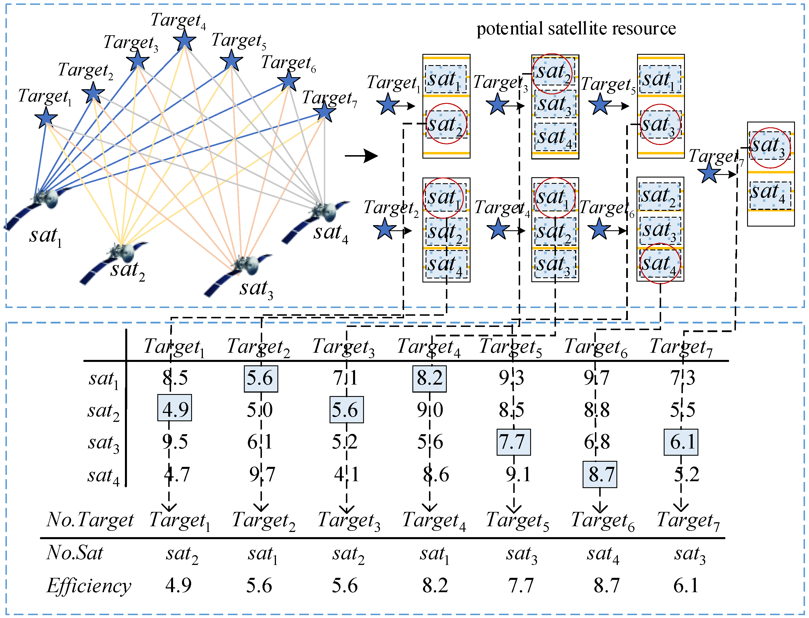
4.1.1. Allocation Optimization Phase

The allocation optimization phase (AOP) is designed to maximize the mission benefit as the optimization goal. Based on the satellite resource set, target mission set, and mission benefit value, several satellite and target mission allocation sequences are matched to form an initial mission planning scheme, which provides a reference sequence for the time window optimization phase. Figure 4 explains the allocation optimization phase’s process in the form of an example. Among them, the red circle represents the selected satellite.

Firstly, for the large-scale target mission scenario where the number of satellites is significantly less than the number of target missions, this section constructs a task benefit repository, which is used to record the task benefit value of each satellite when it performs each target mission, and the task benefit value can be directly called from the task benefit repository to perform the evolution operation during the optimization search process, so as to improve the efficiency of the task assignment and reduce the resource consumption of real-time computation. The mathematical expression of the constructed mission benefit repository is shown in Equation (14):

$$Efficiency(x_{ji})=\left[\begin{array}{c} \begin{array}{ccc}Efficiency(x_{11})& \dots & Efficiency(x_{(1,T)})\\ ⋮& \ddots & ⋮\\ Efficiency(x_{S_{n}1})& \cdots & Efficiency(x_{S_n{N}_T})\\ 0& \cdots & Efficiency(x_{(1,N_T)})\\ ⋮& \ddots & ⋮\\ Efficiency(x_{(S_n,N_T)})& \cdots & 0\end{array}\end{array}\right],$$

(14)

where $Efficiency(x_{ji})$ denotes the mission benefit of $sa{t}_j$ performing $Targe{t}_i$, and $Efficiency(x_{(i,u)})$ denotes the mission benefit of the imaging satellite completing $Targe{t}_i$ and then performs $Targe{t}_i$, starting from $Targe{t}_u$.

Secondly, $N_T$ target tasks are randomly assigned to satellite $S_n$. Theoretically, there is ${(N_T)}^{S_n}$ variety of allocation possibilities, and there is a limitation on the observation demand of the target tasks and the observation capability of the satellites, meaning not every target task can be observed by an arbitrary satellite. Therefore, based on the given target mission set and satellite resource set information, the MSIMPLTS-MLOO model superstructure constraints are invoked to restrict the observation satellites of the target mission, and the potential satellite resource set is filtered to obtain the potential satellite resource set $Sa{t}_{potential}$, so as to achieve an effective reduction in the solution space of the mission planning scheme.

Thereafter, each target task is paired with a randomly selected satellite from its potential satellite resource set; traverses the task benefit repository to obtain the corresponding target task benefit; and takes the execution satellite number, target task number, and its corresponding task benefit as a sequence of satellite and target task assignments and cyclically matches them until all satellites have been assigned to the target task, which constitutes a population separate to several satellites and the sequence of target task assignments. The POM-PSASIDEA algorithm performs an optimization search to generate a sequence allocation scheme that maximizes the mission benefits. The algorithm framework is shown in Algorithm 2.

Algorithm 2. Allocation optimization phase

Input: $obj$ (Parameters of the satellites $S_n$, Parameters of the target task $Task$, Population size $P_n$);

Output: AllocationPlan 1 $Repositor{y}_{Efficiency}=[]$,$Sa{t}_{potential}=[]$;/* initial Task benefit repository and potential satellite resources */ 2 $Repositor{y}_{Efficiency}=Efficiency(x_{ji})$;/* calculate Task benefit repository 3  $Sa{t}_{potential}=Cal{l}_{constraints}(Task,Sat,Constraint{s}_{\mathrm{Superstructure}})$;/* obtain potential satellite resource sets*/ 4  while $G<G_{\max }$ 5   for target = 1:$N_T$ 6   $Sa{t}_{Allocated}=rand(individual.Sa{t}_{potential})$; 7    $Efficienc{y}_{Allocated}=Efficiency(x_{ji})$;/* Traverse Task benefit repository obtain corresponding Efficiency*/ 8 $individual.Sequence=record\_allocation\left(satellite, task, Efficienc{y}_{Allocated},s{t}_k^{i,g}, e{t}_k^{\mathrm{i},g}\right)$; 9   end 10   $InitialAllocation={\displaystyle \sum individual.Sequence}$; 11   $objectiveFunction1=maxEfficiency(Allocation,tasks)$; 12  $AllocationPlan=POM\_PSASIDEA\left(objectiveFunction1, InitialAllocation, parameters\right)$; 13  end

4.1.2. Time Window Optimization Phase

The time window optimization phase (TOP) aims to maximize the task completion rate as the optimization goal through the time window matching rules, which allocate a suitable time window for each target task based on the task planning scheme generated in the allocation optimization phase. The satellite can give priority to the target mission with a high task benefit and early observation start time. Figure 5 illustrates the time window optimization phase in the form of an example.

Firstly, set the assignment task queue to store the observation tasks required by each satellite in descending order of task priority, match the time window for the observation target tasks required by each satellite in the initial task planning scheme one by one according to the time window matching rule, and store the visible time window scheme obtained at this time in $Poo{l}_1$. The target tasks that fail to be allocated and meet the constraints of the mesostructure of the MSIMPLTS-MLOO model are stored in the candidate task queue $candidat{e}_{Task}$ in order of priority from large to small. The time window matching rule considers the priority rule of high-priority tasks and the priority rule of the early start time. In other words, priority is given to assigning visible time windows to target tasks with higher priority and selecting visible time windows with earlier start times to match with target tasks.

Secondly, all free time windows are obtained by traversing the set of satellite visible time windows and the allocated visible time windows, the tasks in the satellite free time windows are randomly assigned to the candidate task queue $candidat{e}_{Task}$, and the POM-PSASIDEA algorithm is used to optimize the search to maximize the task completion degree and store it in $Poo{l}_2$; finally, the visible time window allocation scheme for the satellites and the target task is obtained by considering $Poo{l}_1$ and $Poo{l}_2$ together. In the time window allocation scheme, the idle time window is defined as the remaining visible time window in the satellite visible time window set that has not been allocated. The detailed description is shown in Algorithm 3.

Algorithm 3. Time window optimization phase

Input: AllocationPlan, Parameters of the satellites $Sat$, Parameters of the target task $Task$ Output: $TimeWindowPlan$

1   for j = 1:$S_n$ 2   ${\mathrm{Task}}_{satj}=AllocationPlan(sa{t}_j,Task)$ 3   $task\_queue=sort\left(\left[{\mathrm{Task}}_{satj}.priority\right], ’ascend’\right)$; 4    for i = 1:length($task\_queue$) 5    $Timewindow\_queue=sort(Timewindow,’descend’)$; 6      if $Timewindow$ allocated satisfy the mesostructure of MSIMPLTS-MLOO model constraint 7      $Poo{l}_1=record\_Timewindow\left(task\_queue.idx, Timewindow\_queue.idx\right)$; 8      else 9     $candidat{e}_{Task}=record\_Timewindow\left(task\_queue.idx, Timewindow\_queue.idx\right)$; 10     end 11    end 12 end 13  for $\omega$ = 1:length($Timewindow$) 14    ~any($Timewindow$ (:, 1) $\ge$ visible_windows(i, 1) &$Timewindow$(:, 1) $\le$ visible_windows(i, 2)); 15  $free\_windows=\left[free\_windows; visible\_windows\left(i, :\right)\right]$; 16   if Adjacent but not overlapping $free\_windows=merge(free\_windows(\omega ,\omega +1))$ 17  end 18  $Poo{l}_2=random(free\_windows,candidat{e}_{Task})$,$P_0=Poo{l}_2$; 19  for $G=1:G_{\max }$ 20  $objectiveFunction2=maxTaskAllocationRate\left(P_G, tasks\right)$ 21  $Poo{l}_2=POM\_PSASIDEA\left(objectiveFunction2, P_G, parameters\right)$; 22    $G=G+1$; 23  end 24  $TimeWindowPlan=Poo{l}_1\cup Poo{l}_2$;

4.1.3. Global Optimization Phase

The global optimization phase (GOP) aims to minimize the response time as the optimization objective, consider the planning schemes in the allocation optimization phase and the time window optimization phase, and introduce conflict detection and conflict resolution methods to address the overlap of the planning schemes, so as to generate high-quality mission planning schemes to solve large-scale target scenarios. The high-quality task planning scheme can cope with large-scale target scenarios.

Firstly, the sequential allocation scheme generated in the allocation optimization phase is integrated with the visible time window allocation scheme generated in the time window optimization phase as the initial population $P_0$ for the evolutionary search of the POM-PSASIDEA algorithm, and the population individuals (contemporary mission scenarios) are traversed using a conflict detection method, i.e., by comparing the start times of the time windows of the neighboring missions in the same satellite resource to determine the time window overlap situation (by comparing whether or not intersection exists to judge the time window overlap). If there is a conflict between two neighboring tasks, the higher-priority task is retained, and the lower-priority task is stored in the candidate task queue $candidat{e}_{Task}$, which is treated as a candidate task for reassignment.

Secondly, the conflict elimination method is used to cope with the time window overlap of the planning scheme, the allocated time window of the contemporary mission scheme and the set of satellite visible time windows are matched one by one, the satellite idle time window is screened out, the starting positions of the candidate visible time window and the satellite idle time window are judged one by one according to the priority of the candidate mission queue $candidat{e}_{Task}$, the candidate mission is inserted into the original satellite allocation sequence as a new mission, the successful candidate missions are deleted from the candidate mission queue until the candidate mission queue is empty, and the POM-PSASIDEA algorithm is used for the population individuals. The candidate task is inserted as a new task into the original satellite allocation sequence, and successful candidate tasks are deleted from the candidate task queue. The iteration continues until the candidate task queue is empty. Then, the POM-PSASIDEA algorithm is used to iteratively search for the optimality of the individual populations, and the output is used to generate the final MSIMPLTS-MLOO optimal allocation scheme. The algorithm framework is shown in Algorithm 4.

Algorithm 4. Global optimization phase

Input: $AllocationPlan$, $TimeWindowPlan$, Parameters of the satellites $Sat$, Parameters of the target task $Task$, Population size $P_n$ Output: MSIMPLTS optimal scheme:$finalPlan$

1 $P_0=combinePlans\left(AllocationPlan, TimeWindowPlan\right)$;/* Integration Scheme */ 2  while $G<G_{\max }$ 3    Traverse the integration scheme in $P_G$ 4 if$(e{t}_j^i>s{t}_j^{i+1})\left|\right|[(e{t}_j^i>s{t}_j^{i+1})\&\&(s{t}_j^i<s{t}_j^{i+1}<e{t}_j^{i+1}<e{t}_j^i)]\left|\right|(s{t}_j^i<e{t}_j^{i-1}<s{t}_j^{i+1}<e{t}_j^i)$ 5      $P_G=remove(\min (P_G.Tas{k}_i,P_G.Tas{k}_{i+1}))$; 6      $candidat{e}_{Task}=\min (P_G.Tas{k}_i,P_G.Tas{k}_{i+1})$; 7     else 8      $P_G=P_G$; 9     end 10     $candidat{e}_{Task}=sort(P_G.Task,’descend’)$; 11     $free\_windows=\left[P_G.Timewindow,visible\_windows\left(i, :\right)\right]$; 12   for $h=1:length(candidat{e}_{Task})$ 13      if ~any($P_G.Timewindow$ (:, 1)$\ge$$free\_windows$(i, 1) &$P_G.Timewindow$(:, 1)$\le$ $free\_windows$(i, 2)) 14        if $Timewindow$ allocated satisfy the understructure of MSIMPLTS-MLOO model constraint 15         $individual.P_G=\left\{Task,Sat,free\_windows\left(:, 1\right)\left(i, 2\right)\right\}$; 16       end 17     end 18    end 19     $P_G=P_G\cup individual.P_G$; 20     $objectiveFunction3=minResponseTime\left(P_G\right)$; 21     $G=G+1$; 22   end 23   $finalPlan=POM\_PSASIDEA\left(objectiveFunction3, P_G, parameters\right)$; 24    $G=G+1$; 25  end 26  $TimeWindowPlan=Poo{l}_1\cup Poo{l}_2$;

4.2. Population Size Adaptive Strategy for the Improved Differential Evolution Algorithm

Differential evolution (DE) is an efficient global search algorithm known for its high search efficiency, strong robustness, and fast convergence speed. It is widely used in solving multi-satellite imaging task planning and multi-agent task planning problems [42,43]. When dealing with large-scale target task scenarios, the performance of the algorithm largely depends on the population size. Too large a population size may lead to excessive consumption of computing resources, while too small a population size may lead to premature convergence of the algorithm to the local optimal solution. However, the existing DE algorithm research mainly adopts the alternate use of multiple variation strategies in the optimization process and parameter control to solve problems in the real environment, which is difficult to adapt to the solving requirements of a model at different levels, and there is a risk that feasible solutions cannot be found within the specified time limit. Therefore, this work proposes a population size adaptive strategy for the improved differential evolution algorithm (PSASIDEA) to ensure that the algorithm can solve high-quality task planning schemes while effectively improving the solution efficiency.

Firstly, a population evolution state monitoring mechanism is designed to determine the adjustment of the population size to achieve balanced exploration and utilization of the DE algorithm. In the early stage of algorithm evolution, the population evolution state monitoring mechanism calculates the similarity of individuals within a population and the diversity of individuals between populations to determine whether the algorithm is facing the problem of falling into local optimality and diversity reduction to achieve a reasonable and accurate assessment of the evolution of the population. Based on the distance measure between individuals in the process of population evolution, the calculation method of population individual similarity is derived as shown in Equation (15):

$$\gamma (x_i,x_j)={\displaystyle \frac{1}{\mu +\sqrt{{\displaystyle \sum _{\Omega =1}^{\Omega }{(x_i,x_j)}^2}}}},x_i\ne x_j,$$

(15)

where $x_i$ and $x_j$ denote any two different individuals in the contemporary population, and $\Omega$ denotes the parameter dimensions; to avoid the instability of similarity $\gamma$, a small positive number $\mu$ is introduced to smooth the values.

Afterwards, we constructed a method for calculating individual diversity among populations, with the mathematical expression shown in Equation (16):

$$\xi (P_{history}^g,P_{current})={\displaystyle \frac{{\displaystyle \sum _{i=1}^{N_{history}^g}{\displaystyle \sum _{j=1}^{N_{current}}\sqrt{{\displaystyle \sum _{i=1}^{\Omega }{(x_i,x_j)}^2}}}}}{N_{history}^g\cdot N_{current}}},\forall x_i\in P_{history}^g,x_j\in P_{current},$$

(16)

where $P_{history}^g$ denotes the $g$-th iteration population in the historical environment, $P_{current}$ denotes the current population, $N_{history}^g$ denotes the number of individuals in population $P_{history}^g$, $N_{current}$ denotes the number of individuals in population $P_{current}$, and $x_i$ and $x_j$ denote the individuals in population m and population n, respectively.

We construct the similarity matrix to measure the similarity degree among individuals in a population and store the population individual similarity calculated in each iteration into the similarity matrix as historical data. The similarity matrix constructed is shown in Equation (17):

$$S=\left[\begin{array}{cccc}1& \gamma (x_1,x_2)& \dots & \gamma (x_1,x_n)\\ 1& 1& \dots & \gamma (x_2,x_n)\\ ⋮& ⋮& \ddots & ⋮\\ 1& 1& \cdots & 1\end{array}\right],$$

(17)

Thereafter, after storing the historical data based on the similarity matrix, the Upper Quartile (UQ) is selected as the population individual similarity threshold $Q_{\gamma }$, and all the values greater than or equal to the threshold are considered as having high similarity, while values less than the threshold are considered as having low similarity. Similarly, the diversity matrix is obtained, and the diversity threshold is $Q_{\xi }$.

It is worth noting that individual similarity within a population is used to assess the degree of similarity of individuals within a population, focusing on the differences between individuals. Population diversity is used to assess the overall level of variation in the population. The calculation of individual similarity and population diversity enables a comprehensive evaluation of both dimensions of the algorithm.

In the later stages of algorithm evolution, the population evolution status monitoring mechanism determines whether the algorithm is facing evolutionary stagnation through both the fitness value and the population evolution rate. Here, the fitness value is consistent with the objective function of each layer of the MSIMPLTS-MLOO model, and the population evolution rate refers to the degree of improvement in the optimal solution between two adjacent generations, which can reflect the convergence speed of the population to a certain extent. The mathematical expression for the population evolution rate is shown in Equation (18):

$$R_{evolution}={\displaystyle \frac{1}{0.5G}}{\displaystyle \sum _{g=0.5G}^G\frac{f_i(optima{l}_g)-f_i(optima{l}_{g-1})}{|f_i(optima{l}_{g-1})|+\mu }},i=(1,2,3)$$

(18)

where the population evolution rate is calculated at the late stage of evolution, so the number of iterations after 50% is $[0.5G,G]$, $G$ denotes the number of iterations, $g$ denotes the current number of iterations, and $f_i(optima{l}_g)$ denotes the value of optimal fitness among the populations in the $g$-th generation of the $i$-th objective function of the MSIMPLTS-MLOO model. If the population evolution rate is not significantly improved in generation $m$, it can be assumed that there is a stagnation problem in the population evolution.

Secondly, according to the output results of the population evolution state monitoring mechanism, the population size adaptive strategy is used to adjust the population size. For the pre-evolutionary stage of the algorithm, there is a high similarity and low diversity of individual populations, and there is an adaptive increase in population size to improve the diversity of the population, which is conducive to promoting the exploration of the algorithm to help it jump out of the local optimum; for the late stage of the algorithm, there is a stagnation of the value of the fitness of the population, as well as the rate of evolution of the population for many consecutive generations; adaptive reduction in the population size is conducive to the depth of the development to accelerate the rate of convergence of the population. The construction method of the population size adaptive strategy is shown in Equation (18):

$$\left\{\begin{array}{l}{N}_g=N_{initial}+(N_{max}-N_{initial})\cdot {\displaystyle \frac{f_i(x)}{\max f_i(x)}},g\in [0,0.5G]\\ N_g=N_{0.5G}-(N_{0.5G}-N_{min})\cdot {\displaystyle \frac{f_i(x)}{\max f_i(x)}},g\in [0.5G,G]\end{array}\right.$$

(19)

where $N_g$ denotes the population size of the $g$-th iteration, $N_{max}$ and $N_{min}$ denote the upper and lower limits of the population size, respectively, and $f_i(x)/\max f_i(x)$ denotes the ratio of the fitness value of the objective function to the maximum fitness value of the previous generations, which is used as a scaling factor for the adjustment of the population size.

Since too large a population size may lead to excessive consumption of computational resources, while too small a population size may lead to premature convergence of the algorithm to a local optimum, the upper and lower values of the population size are set to enable the algorithm to achieve a balance between stability and robustness.

The PSASIDEA algorithm is specifically described in Algorithm 5. Firstly, a random population is generated based on the initial population size, and in each iteration of the generation, a mutation operation is performed to generate new mutated individuals. Then, a crossover operation is applied to generate test individuals, followed by a selection operation to decide which individuals will enter the next generation of the population. After each generation iteration, the population evolution status is evaluated based on the population evolution monitoring mechanism, and a new population is created based on the algorithm’s performance and robustness. After each iteration, the population evolutionary state is evaluated according to a corresponding monitoring mechanism, and the population size is adjusted according to the performance of the algorithm and the search state.

Algorithm 5. Population size adaptive strategy for the improved differential evolution algorithm

Input: $AllocationPlan$, $TimeWindowPlan$, Parameters of the satellites $Sat$, Parameters of the target task $Task$, Population size $P_n$ Output: MSIMPLTS optimal scheme: $finalPlan$

1  /* Initialization parameter*/ 2   $N=N_{\min }$; 3    $Pop=InitializePopulation\left(N, D\right)$; /*Initial population*/ 4      while $G<G_{\max }$ 5      $Newpop=mutation(Pop)\&crossover(Pop)$; 6      $Pop=selection(Newpop,Pop)$; /*update population*/ 7      $[fitness,best\_idx]=\max (Pop.individual.fitness)$;/*update optimal fitness*/ 8       if $G<G_{\max }/2$ 9       Calculate Population individual similarity $\gamma (x_i,x_j)$ by using Equation (15); 10     Calculate individual diversity $\xi (P_{history}^g,P_{current})$ between populations by using Equation (16); 11           if $(\gamma (x_i,x_j)\ge Q_{\gamma })\&(\xi (P_{history}^g,P_{current})\le Q_{\xi })$ 12           $N_g=N_{initial}+(N_{max}-N_{initial})\cdot {\displaystyle \frac{f_i(x)}{\max f_i(x)}}$; 13          else 14          $N_g=N_{initial}$; 15          end 16     else 17     Calculate population evolution rate $R_{evolution}$ by using Equation (17); 18          if The population evolution rate $R_{evolution}$ stagnated more than $m$ generations 19         $N_g=N_{0.5G}-(N_{0.5G}-N_{min})\cdot {\displaystyle \frac{f_i(x)}{\max f_i(x)}}$ 20          else 21            $N_g=N_{initial}$; 22          end 23      end 24      $G=G+1$; 25  end 26  $finalPlan=POM\_PSASIDEA\left(objectiveFunction, P_G, parameters\right)$;

5. Experimental Results and Analysis

To verify the effectiveness and stability of the POM-PSASIDEA algorithm to solve MSIMPLTS, this work set up three sets of simulation experiments. Experiment 1: POM-PSASIDEA algorithm resolves MSIMPLTS effectiveness. Experiment 2: POM-PSASIDEA algorithm resolves MSIMPLTS scalability. Experiment 3: POM-PSASIDEA algorithm performance analysis.

5.1. Subsection Experimental Setting

The experiment used eight imaging satellites from the simulation scenario set up by the Satellite Toolkit (STK), and the simulation time was set from 18 June 2024 04:00:00 (UTCG) to 19 June 2024 04:00:00 (UTCG). The orbital parameters of the eight imaging satellites and the parameters of the payloads are listed in

Table 1. Satellite orbit parameters and satellite payload parameters.

No. Sat	$\mathit{a}$ /(km)	$\mathit{e}$ /(°)	$\mathit{i}$ /(°)	$\mathit{R}\mathit{A}\mathit{A}\mathit{N}$ /(°)	$\mathit{\omega }$ /(°)	$\mathit{\phi }$ /(°)	${\mathit{\theta }}_{\mathit{j}}$ /(°)	$\mathit{t}{\mathbf{max}}_{{\mathit{S}}_{\mathit{j}}}$ /(s)	${\mathit{A}}_{\mathit{j}}$ (°)	${\mathit{w}}_{\mathit{j}}$ /(°/s)	${\mathit{r}}_{\mathit{j}}^{\mathit{s}}$ /(m)
Sat1	6871	0.013	98.54	179	94.764	109.153	6	400	30	0.2	2
Sat2	6871	0.021	97.42	159	97.034	122.516	6	400	30	0.2	2
Sat3	6871	0.016	90.32	139	90.972	162.317	6	400	30	0.2	2
Sat4	6871	0.014	98.50	119	92.612	119.562	6	450	30	0.3	2
Sat5	6871	0.037	97.90	99	92.860	157.373	7	450	35	0.3	2
Sat6	6871	0.028	96.31	79	92.172	188.254	7	450	35	0.3	1.5
Sat7	6871	0.055	97.44	59	97.629	172.768	8	500	35	0.3	1.5
Sat8	6871	0.051	90.65	29	93.795	103.553	8	500	35	0.4	1.5

. Among them, the satellite orbital parameters include the half-length axis length ($a$), eccentricity ($e$), orbital inclination ($i$), perigee spoke angle ($\omega$), ascending node ruddy longitude ($RAAN$), and true proximity angle ($\phi$), and the payload parameters include the field-of-view (${\theta }_j$), single longest on-time ($t{\max }_{S_j}$), maximum side-swinging angle ($A_j$), average side-swinging rate ($w_j$), and optimal resolution ($r_j^s$). The parameters of the POM-PSASIDEA algorithm were set with a crossover rate of 0.5, a mutation rate of 0.6, initial population size of 100 (adaptively adjusted according to the method in Section 4.2), and maximum number of iterations of 1000 generations.

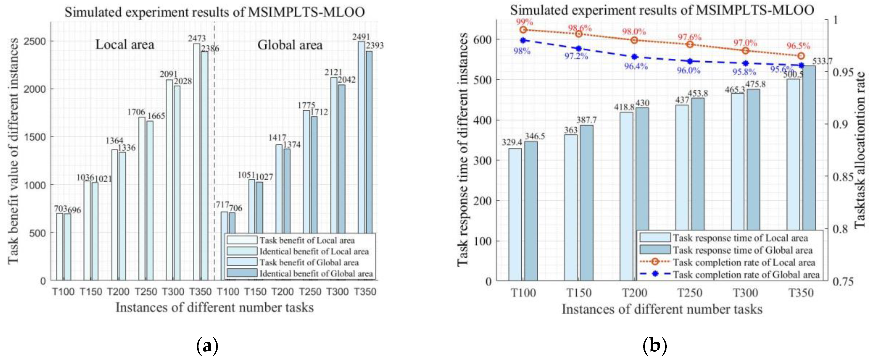
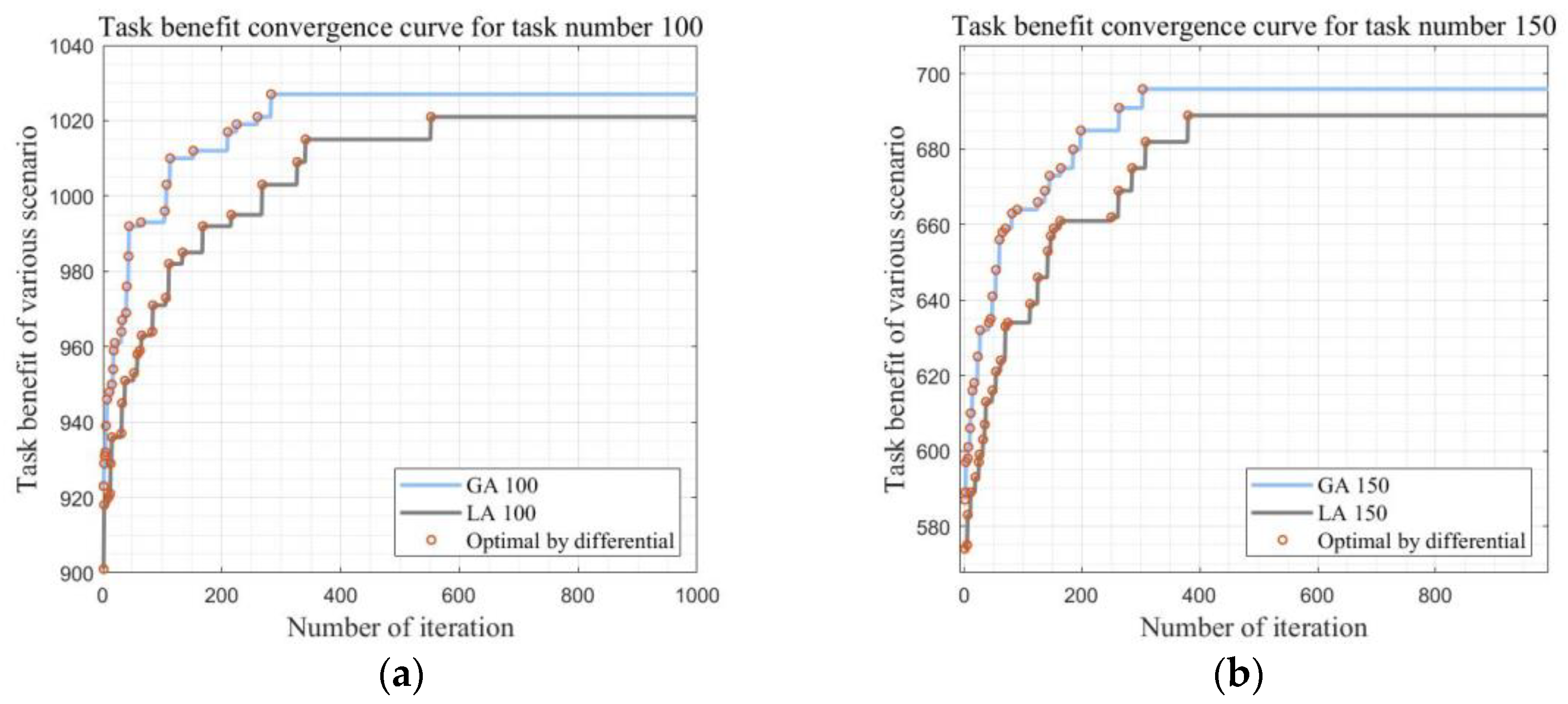
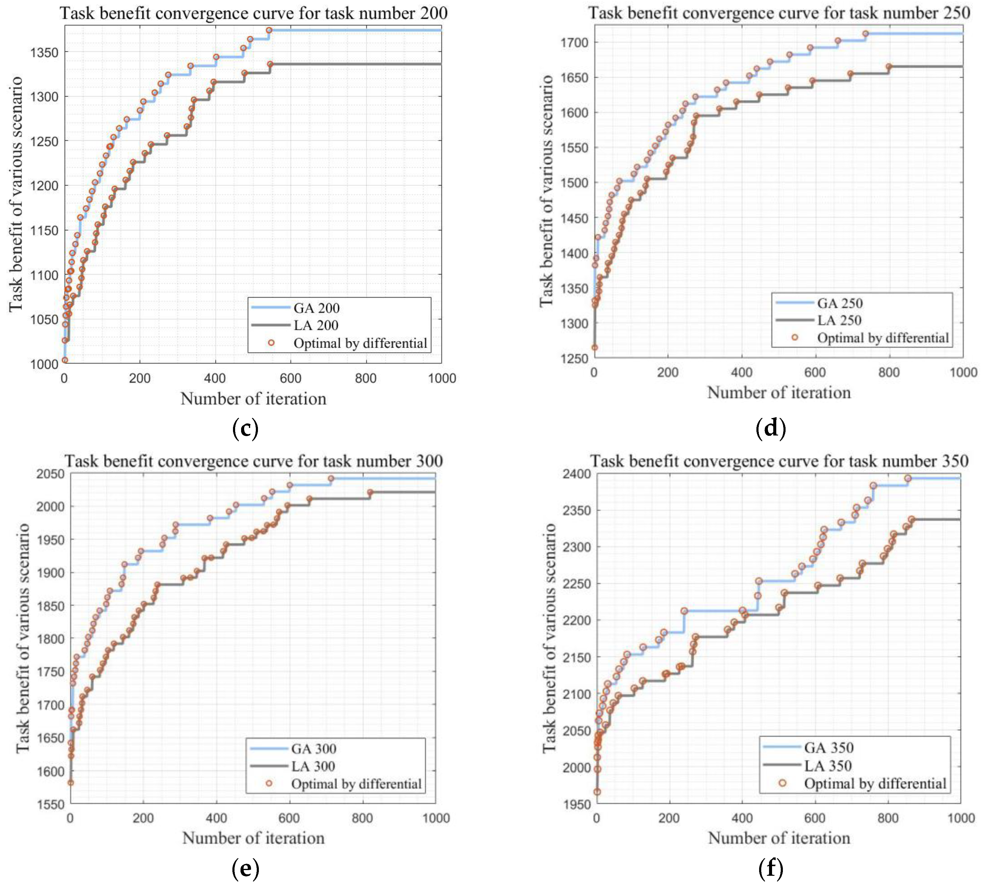
5.2. Experiment 1: POM-PSASIDEA Algorithm Resolves MSIMPLTS Effectiveness

To verify the effectiveness of the POM-PSASIDEA algorithm in processing MSIMPLTS, this experiment generated 100 target tasks uniformly in a local range of longitude [75, 135] and latitude [20, 50], which was used to simulate the task requirements in a large-scale target scenario. The geographic distribution of the 100 target tasks is shown in Figure 6.

Firstly, the POM-PSASIDEA algorithm was used to solve the MSIMPLTS model under 100 target scenarios, and the allocation optimization stage matched several satellite and target task allocation sequences to form an initial task planning scheme based on the satellite resources and target task information. The initial planning results are shown in

Table 2. Simulated experimental results of the allocation optimization phase.

T	1	2	3	4	5	6	7	8	9	10	11	12	13	14	15	16	17	18	19	20
Sat	5	6	1	7	2	3	8	7	4	5	4	6	8	2	6	3	1	3	7	6
E	8	7	6	4	8	9	8	8	6	5	6	6	9	7	9	5	8	6	5	9
T	21	22	23	24	25	26	27	28	29	30	31	32	33	34	35	36	37	38	39	40
Sat	1	7	5	3	4	2	7	1	8	2	3	8	5	7	6	1	7	4	2	6
E	5	4	7	5	6	7	6	6	5	5	7	9	8	5	4	5	3	6	4	8
T	41	42	43	44	45	46	47	48	49	50	51	52	53	54	55	56	57	58	59	60
Sat	7	1	2	5	3	4	6	1	8	7	8	1	2	5	8	3	7	4	6	8
E	8	3	9	7	6	3	4	8	9	7	9	5	6	7	4	8	7	4	6	8
T	61	62	63	64	65	66	67	68	69	70	71	72	73	74	75	76	77	78	79	80
Sat	1	7	6	3	4	2	6	8	5	2	5	4	7	1	3	5	8	4	6	8
E	4	5	8	9	9	7	7	8	6	5	3	5	4	5	5	9	5	5	7	9
Target	81	82	83	84	85	86	87	88	89	90	91	92	93	94	95	96	97	98	99	100
Sat	4	3	2	5	8	7	4	6	1	7	2	3	5	2	6	8	4	5	1	3
E	7	9	6	7	4	9	9	5	7	4	5	8	5	4	4	6	8	5	9	3

, where “T” denotes the target mission number, “Sat” denotes the satellite number, and E denotes the mission benefit.

Based on the initial mission planning scheme shown in Table 2, the distribution relationship between the executing satellites and the target missions was visualized as shown in Figure 7. This figure represents the grouped bars of the initial mission planning scheme, with each group of sub-bars corresponding to a satellite (Satellite 1 to Satellite 8), where the x-axis represents the target mission number and the y-axis represents the target mission benefit.

Combining Table 2 and Figure 7, it can be seen that all 100 target tasks are effectively assigned in the assignment optimization phase, and the POM-PSASIDEA algorithm can effectively solve the MSIMPLTS-MLOO superstructure model to generate the initial mission planning scheme containing the satellite and target task assignment sequences.

After that, it enters the time window optimization phase to allocate appropriate time windows for each target mission based on the initial mission planning scheme.

Table 3. Simulated experimental results of the time window optimization scheme phase.

T	St	Et	T	St	Et	T	St	Et	T	St	Et
T1	16:35:34	16:38:54	T26	19:41:38	19:43:50	T51	00:22:34	00:27:07	T76	12:12:20	12:14:12
T2	22:15:26	22:17:47	T27	19:41:38	19:43:50	T52	17:23:38	17:24:36	T77	23:43:21	23:47:16
T3	20:26:49	20:27:17	T28	04:00:00	04:03:23	T53	05:05:38	05:08:36	T78	07:42:53	07:45:03
T4	19:22:14	19:25:34	T29	16:36:26	16:38:40	T54	14:10:47	14:13:11	T79	04:38:34	04:40:52
T5	11:04:41	11:06:16	T30	12:57:50	13:01:00	T55	18:33:15	18:40:27	T80	12:29:36	12:31:55
T6	06:20:24	06:22:00	T31	16:28:02	16:32:15	T56	01:10:03	01:16:53	T81	03:08:00	03:12:01
T7	18:34:31	18:41:45	T32	21:39:51	21:43:06	T57	01:51:31	01:58:47	T82	12:43:23	12:45:48
T8	08:06:47	08:08:56	T33	19:19:48	19:23:09	T58	13:34:30	13:37:36	T83	03:02:25	03:04:22
T9	02:47:24	02:49:43	T34	03:48:16	03:55:19	T59	20:10:24	20:16:55	T84	10:56:14	11:00:01
T10	11:30:27	11:32:19	T35	06:17:34	06:19:54	T60	06:28:54	06:31:13	T85	11:06:20	11:12:44
T11	14:17:07	14:18:59	T36	04:00:00	04:04:19	T61	17:32:30	17:35:41	T86	14:20:49	14:23:14
T12	02:22:44	02:25:37	T37	00:10:40	00:16:36	T62	20:36:05	20:38:03	T87	06:53:16	06:56:07
T13	12:55:33	12:57:45	T38	12:39:35	12:41:50	T63	16:04:37	16:06:46	T88	15:14:17	15:16:34
T14	10:59:22	11:01:13	T39	03:29:17	03:34:52	T64	01:26:30	01:29:21	T89	01:53:20	02:00:40
T15	00:53:08	00:56:29	T40	11:10:18	11:12:39	T65	06:26:29	06:28:34	T90	01:56:14	01:58:18
T16	15:14:48	15:20:08	T41	16:17:02	16:21:31	T66	15:54:28	15:56:04	T91	09:33:09	09:35:00
T17	14:16:45	14:24:00	T42	09:25:40	09:27:32	T67	20:02:46	20:05:30	T92	15:30:03	15:32:28
T18	07:02:35	07:05:37	T43	17:06:50	17:12:23	T68	07:27:19	07:34:22	T93	17:26:06	17:28:06
T19	12:39:44	12:47:04	T44	07:58:05	08:04:57	T69	03:03:12	03:05:35	T94	07:39:16	07:46:39
T20	01:26:19	01:33:35	T45	20:31:33	20:33:42	T70	05:56:33	05:58:39	T95	23:17:12	23:19:51
T21	05:47:29	05:53:38	T46	12:18:17	12:20:35	T71	14:46:43	14:50:11	T96	03:08:56	03:11:21
T22	13:34:05	13:36:33	T47	22:22:59	22:23:26	T72	10:12:24	10:15:40	T97	01:38:46	01:40:19
T23	06:00:56	06:07:44	T48	14:54:37	15:01:20	T73	04:11:12	04:13:29	T98	21:52:57	21:57:37
T24	11:36:34	11:39:09	T49	10:31:17	10:33:26	T74	23:46:30	23:48:07	T99	16:38:35	16:41:21
T25	17:52:10	17:53:19	T50	23:35:08	23:37:21	T75	21:33:47	21:40:44	T100	14:09:03	14:12:14

shows the time window allocation scheme in the time window optimization phase, where “T” denotes the target mission number, “St” denotes the time window observation start time, and “Et” denotes the time window observation end time. Table 3 shows that all 100 target tasks are assigned to visible time windows, and the time window optimization phase can assign a visible time window to each target task for observation.

Finally, the global optimization phase considers the planning schemes from both the allocation optimization phase and the time window optimization phase and employs a conflict detection method to evaluate the contemporary task planning schemes. There is a certain degree of time window overlap among the contemporary task planning schemes, where the overlapping parts are tasks T28 and T36, T7 and T55, and T57 and T90. We adopt the conflict elimination method to deal with the overlapping time windows of the planning schemes, and we generate the final MSIMPLTS-MLOO task planning schemes through the POM-PSASIDEA algorithm by iteratively searching for the optimal contemporary mission planning schemes, as shown in Figure 8.

Figure 8 presents the allocation schematic of the final MSIMPLTS-MLOO mission planning scheme, where the x-axis indicates the mission planning time, the y-axis indicates the satellite number, eight rectangles of different colors are used to indicate the target tasks assigned to different satellites, the width of the rectangles indicate the range of the satellite’s observation time window, and the red dashed boxes are marked as the target tasks that are reallocated using the conflict cancellation method. As can be seen in Figure 8, the POM-PSASIDEA algorithm provides an effective allocation of the visible time window for eight satellites with 100 target tasks.

The Experiment 1 simulation results show that the POM-PSASIDEA algorithm proposed in this work can solve the MSIMPLTS-MLOO model effectively in large-scale target task scenarios, and the use of the allocation optimization, time window optimization, and global optimization phases of the progressive optimization mechanism can generate the final mission plan effectively for large-scale target task scenarios. Therefore, the POM-PSASIDEA algorithm solution has MSIMPLTS effectiveness.

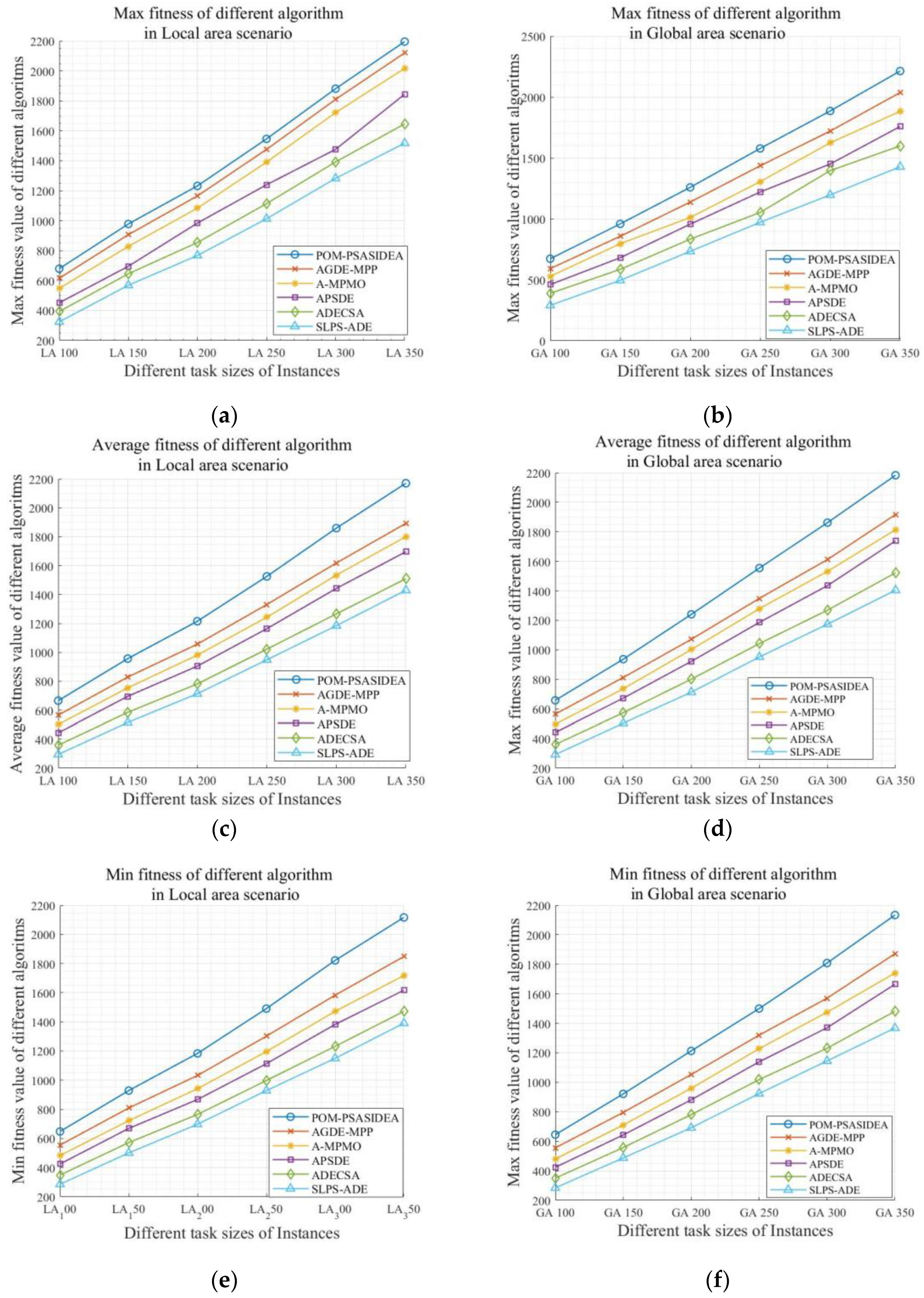
5.3. Experiment 2: POM-PSASIDEA Algorithm Resolves MSIMPLTS Scalability

To further verify the stability of the POM-PSASIDEA algorithm for solving MSIMPLTS, multiple sets of instances at different scales were used to verify the performance of the algorithm. For the local region of longitude [75, 135] and latitude [20, 50] and the global region of longitude [−180, 180] and latitude [−90, 90], instances with 100, 150, 200, 250, 300, and 350 target tasks were generated with a random distribution; a total of 12 groups of instances were generated for the simulation experiments.

The experimental results of the POM-PSASIDEA algorithm for solving different task size instances of MSIMPLTS in large-scale target task scenarios are shown in

Table 4. Simulated experimental results for the POM-PSASIDEA algorithm solved in different instances.

Instance	S	T	${\mathit{I}}_{\mathit{E}\mathit{f}\mathit{f}\mathit{i}\mathit{c}\mathit{i}\mathit{e}\mathit{n}\mathit{c}\mathit{y}}$	$\mathit{E}\mathit{f}\mathit{f}\mathit{i}\mathit{c}\mathit{i}\mathit{e}\mathit{n}\mathit{c}\mathit{y}$	${\mathit{R}}_{\mathit{a}\mathit{l}\mathit{l}\mathit{o}\mathit{c}\mathit{a}\mathit{t}\mathit{i}\mathit{o}\mathit{n}}$	$\mathit{T}\mathit{i}\mathit{m}{\mathit{e}}_{\mathit{r}\mathit{e}\mathit{s}}$
LA_100	8	100	703	696	99.0%	329.4
GA_100	8	100	717	706	98.6%	346.5
LA_150	8	150	1036	1021	98.6%	363.0
GA_150	8	150	1051	1027	97.8%	387.7
LA_200	8	200	1364	1336	98.0%	418.8
GA_200	8	200	1417	1374	97.0%	430.0
LA_250	8	250	1706	1665	97.6%	437.0
GA_250	8	250	1775	1712	96.5%	453.8
LA_300	8	300	2091	2028	97.0%	465.3
GA_300	8	300	2121	2042	96.3%	475.8
LA_350	8	350	2473	2386	96.5%	500.5
GA_350	8	350	2491	2393	96.1%	533.7

. “$I_{Efficiency}$” denotes the task benefit in the ideal case, “$Efficiency$” denotes the task benefits in the actual case, “$R_{allocation}$” denotes the task assignment rate, and “$Tim{e}_{res}$” denotes the response time. The local area and global area simulation instances are represented by LA_Number and GA_Number, respectively, where Number is the number of target tasks. Note that, since the target tasks were randomly generated, the ideal task benefits are different in each instance.

Figure 9 shows the performance analysis of the MSIMPLTS-MLOO model for different instances of large-scale target mission scenarios, specifically six sets of instances with the number of target missions of 100, 150, 200, 250, 300, and 350 under the local region and the global region. Figure 9a shows the mission benefits in the local and global regions. With the increase in the number of satellites and targets, the mission benefits in the local region are always higher than those in the global region, which is because, in the local region, since the target tasks are relatively concentrated, the model can schedule the satellite resources more efficiently and prioritize the demand for high-priority tasks, thus achieving higher mission benefits. Figure 9b illustrates the mission response time and mission allocation rate. With the increase in the number of satellites and targets, the mission response time increases slightly in the instances within the local region and global region, but the increase is more moderate. In addition, the task allocation rate has not decreased significantly in each group of instances and has always been maintained at a high level, which indicates that the MSIMPLTS-MLOO model has high efficiency and stability in resource allocation and can ensure that most of the tasks can be allocated to satellites for execution in a timely and effective manner. Figure 9 shows that, as the number of satellites and targets increases, the MSIMPLTS-MLOO model is still able to achieve a fast response to the mission planning scenarios when dealing with MSIMPLTS and performs excellently in terms of mission benefits and mission allocation rates.

In addition, Figure 10 illustrates the convergence of the POM-PSASIDEA algorithm in terms of task benefits for different task sizes (100 to 350).

Examples are given in Figure 10a–f for the task sizes of 100, 150, 200, 250, 300, and 350, respectively. The blue line segments indicate the convergence of task benefits in the global region, the black line segments indicate the same on a local scale, and the red circles indicate the difference-seeking points.

As can be seen from Figure 10, instances with task sizes ranging from 100 to 350 in both the local and global regions show good convergence characteristics despite different task planning and simulation scenarios. In addition, the task convergence curves of each sub-figure show that the task benefit gradually converges to stability with the increase in the number of iterations of the algorithm, and the red circles in the figure illustrate the distribution of the differential search points. With the increase in the number of iterations, the search points are intensive in the early stage of the algorithm’s evolution, while the convergence gradually decreases in the middle and late stages of the evolution, which reflects the POM-PSASIDEA algorithm at different stages of the optimization search adaptively adjusting the population size to balance the exploratory and exploitative nature to approach the local optimal solution faster and search for a high-quality task planning scheme.

The simulation results of Experiment 2 show that the POM-PSASIDEA algorithm proposed in this work can effectively solve the MSIMPLTS-MLOO model in large-scale target task scenarios, and with an increase in the task size, it can solve the task planning scheme in a shorter time with a higher task benefit and task allocation rate. As such, the POM-PSASIDEA algorithm solves MSIMPLTS with stability.

5.4. Experiment 3: POM-PSASIDEA Algorithm Performance Analysis

In this section, we present how the proposed POM-PSASIDEA algorithm was judged against the AGDE-MPP algorithm [44] (Adaptive Guided Differential Evolution Algorithm on Mutation, Parameter, and Population), A-MPMO algorithm [45] (Adaptive Strategy with A Multi-population Multi-objective Algorithm), APSDE [46] (Adaptive Parameter and Strategy with Differential Evolution Algorithm), ADECSA [47] (Adaptive Clonal Selection Algorithm with Multiple Differential Evolution Strategies), and SLPS-ADE [48] (Sawtooth Linear Population Size-based Adaptive Differential Evolution) to compare the performance levels of these five algorithms. A detailed description of the algorithms is given in Appendix B, which includes the main characteristics and applicable scenarios of each algorithm.

The POM-PSASIDEA, AGDE-MPP, A-MPMO, ADECSA, and SLPS-ADE algorithms were applied for the MSIMPLTS problem in the local and global regions, with the number of target tasks set as 100, 150, 200, 250, 300, and 350, and the results of the experiments are shown in

Table 5. Simulated experiment results of the POM-PSASIDEA algorithm in different instances.

Instances	POM-PSASIDEA			AGDE-MPP			A-MPMO
	${\mathit{f}}_{\mathbf{max}}$	${\mathit{f}}_{\mathit{a}\mathit{v}\mathit{g}}$	${\mathit{f}}_{\mathbf{min}}$	${\mathit{f}}_{\mathbf{max}}$	${\mathit{f}}_{\mathit{a}\mathit{v}\mathit{g}}$	${\mathit{f}}_{\mathbf{min}}$	${\mathit{f}}_{\mathbf{max}}$	${\mathit{f}}_{\mathit{a}\mathit{v}\mathit{g}}$	${\mathit{f}}_{\mathbf{min}}$
LA_100	479.6	465.6	447.8	446	415.7	404.5	417.6	401.5	382.8
LA_150	778.1	756.6	728.7	728.1	678.9	659.2	667.1	654	621.9
LA_200	1032.2	1015.2	983.7	967.6	906.5	882.5	924.9	880.9	841.6
LA_250	1346.0	1325.6	1290.9	1264.3	1180.9	1151.6	1222.5	1142.5	1095.8
LA_300	1681.2	1659.7	1621.7	1571.6	1468.3	1432.9	1578.2	1434.7	1372.3
LA_350	1995.6	1970.3	1916.7	1865.9	1742.8	1698.2	1734.7	1700.7	1617.7
Avg	1218.7	1198.8	1164.9	1140.5	1065.5	1038.2	1090.8	1035.7	988.7
GA_100	473.2	458.1	445.2	442.2	414.8	405.8	428.8	397	380.3
GA_150	759.1	737.1	721.6	707.2	663.2	646	696.7	636.7	610.7
GA_200	1059.0	1041.0	1012.7	988	921.8	902.9	911.3	902.3	859
GA_250	1378.0	1354.7	1299.9	1285.7	1199.1	1169.5	1205.9	1179.5	1127.8
GA_300	1685.3	1662.5	1608.4	1570.3	1462.3	1420.1	1524.4	1432.4	1375.1
GA_350	2013.2	1983.6	1934.0	1886.4	1767.4	1721.7	1782.3	1713.9	1640.7
Avg	1227.9	1206.1	1170.3	1146.6	1071.4	1044.3	1091.6	1043.6	998.9
Instances	APSDE			ADECSA			SLPS-ADE
	${\mathit{f}}_{\mathbf{max}}$	${\mathit{f}}_{\mathit{a}\mathit{v}\mathit{g}}$	${\mathit{f}}_{\mathbf{min}}$	${\mathit{f}}_{\mathbf{max}}$	${\mathit{f}}_{\mathit{a}\mathit{v}\mathit{g}}$	${\mathit{f}}_{\mathbf{min}}$	${\mathit{f}}_{\mathbf{max}}$	${\mathit{f}}_{\mathit{a}\mathit{v}\mathit{g}}$	${\mathit{f}}_{\mathbf{min}}$
LA_100	401.8	393.9	374.8	370.2	359.4	348.9	350.4	345.2	335.8
LA_150	697.2	645.6	618.8	614.1	584.9	571.7	573.1	565.6	550.8
LA_200	931.3	854.4	817.5	851.7	781.4	764.8	771.4	763.6	747.7
LA_250	1189.7	1113.7	1062.8	1093.3	1021.8	997.5	992.6	998.2	978.2
LA_300	1476.2	1392.6	1332.3	1342.5	1266.5	1232	1234.1	1234.7	1199.6
LA_350	1794.4	1646.3	1567	1540	1509.6	1472.3	1492	1480	1441
Avg	1081.8	1007.8	962.2	968.6	920.6	897.9	902.3	897.9	875.5
GA_100	411.3	391.7	374.1	389.4	360.6	350.6	341	342.3	334.7
GA_150	631.4	623.2	593.3	586	574.4	557.8	546.1	554	537.4
GA_200	907.1	872.2	831.2	833.8	801.7	780.8	783.8	763.5	741.6
GA_250	1170.5	1136.4	1088.6	1053	1042.6	1018.4	1022.3	1001.9	973.8
GA_300	1400.5	1385.7	1319.8	1396.1	1269.2	1231.1	1246.9	1224.2	1194.9
GA_350	1858.2	1689.3	1614.8	1599	1522.8	1481.7	1477.8	1454.5	1417.8
Avg	1063.2	1016.4	970.3	976.2	928.6	903.4	903.0	890.1	866.7

and Figure 11.

To comprehensively evaluate the performance of the POM-PSASIDEA algorithm and other algorithms in solving the MSIMPLTS problem, we used the optimal fitness value $f_{\max }$, average fitness value $f_{avg}$, and worst fitness value $f_{\min }$ as the evaluation indexes, where the optimal fitness value $f_{\max }$ reflects the optimal solution for the population, the average fitness value $f_{avg}$ reflects the fitness value level of the population as a whole, and the worst fitness value $f_{\min }$ reflects the existence of the worse solution for the population (or falling into the worst fitness value reflects whether the population has a poor solution or falls into local optimality).

In Table 5 and Figure 11, it can be seen that the POM-PSASIDEA algorithm has higher optimal fitness values $f_{\max }$ than the other algorithms in different task size instances in the local and global area scenarios, which indicates that the population size adaptive strategy of the POM-PSASIDEA algorithm is effective in the optimization search process and can trade off exploratorily and exploitatively guiding the algorithm to quickly search for the optimal task planning scheme. Meanwhile, the POM-PSASIDEA algorithm outperforms the other algorithms in terms of the average $f_{avg}$ and worst fitness values $f_{\min }$, and the superiority of the average fitness value $f_{avg}$ indicates that its overall population fitness level is improved. Moreover, the superiority of the worst fitness value $f_{\min }$ indicates that there are fewer poor solutions in the population, and its adaptive adjustment of the population size effectively avoids the problem of falling into the local optimum.

The results of Experiment 3 show that the POM-PSASIDEA algorithm exhibits higher optimal fitness values and average fitness values than the other five algorithms in solving the MSIMPLTS problem, and at the same time, it can effectively avoid falling into the local optimum and maintain a high population diversity. Therefore, the POM-PSASIDEA algorithm is superior for solving the multi-satellite imaging mission planning problem for large-scale target missions.

6. Discussion

In this section, firstly, the proposed progressive optimization mechanism and population size adaptive strategy for the improved differential evolution algorithm (POM-PSASIDEA) and its simulation results are discussed in depth, focusing on the scalability of the model design, the superiority of the algorithm, and the effectiveness of the recursive optimization mechanism. Secondly, the limitations of the current study and future research directions are discussed.

6.1. Discussion of the Current Research

• Scalability of MSIMPLTS based on Multi-layer Objective Optimization

The MSIMPLTS model based on Multi-layer Objective Optimization (MSIMPLTS-MLOO) provides strong scalability and adaptability by setting up an upper, middle, and lower layer structure to handle different optimization objectives in layers. Specifically, the MSIMPLTS-MLOO model is relatively independent among the layers and can flexibly cope with MSIMPLTS problems with different target task sizes through the adaptive adjustment of optimization objectives and constraints in each layer. In addition, the hierarchical processing of the model effectively reduces the complexity of the problem, and the layer-by-layer optimization enables the objective function and constraints of each layer to be optimized in a more precise range, thus avoiding the computational complexity and local optimal solution problems that may occur in global optimization. Through the simulation experiments of the MSIMPLTS-MLOO model, it can be seen that the MSIMPLTS-MLOO model is able to maintain a fast response with the increase in the number of satellites and targets when processing MSIMPLTS, and it also has excellent performance in terms of the mission benefit.

2.

Effectiveness of the progressive optimization mechanism

The construction of a progressive optimization mechanism makes the mission planning process more orderly and systematic. In the allocation optimization phase, the allocation sequences of satellites and target tasks are generated by considering the objective function of maximizing the mission revenue, so that effective allocation of satellite resources can be achieved. Then, in the time window optimization phase, according to the decision scheme in the allocation optimization phase, a feasible observation time window is assigned to each target mission with the objective function of maximizing the mission allocation rate so as to reduce the possibility of mission conflict. Finally, minimizing the response time objective function is further considered in the global optimization phase, which integrates the decision results of the previous two phases to output a task planning scheme adapted to the current environment. Simulation experiments show that the progressive optimization mechanism, which divides the optimization process into three phases, enables the algorithm to gradually refine the planning scheme and thus more dynamically adjust for different optimization objectives in each phase, improving the overall quality of the planning scheme and the practical application effect and making it adaptable to task scenarios of different scales and complexities.

3.

Superiority of the population size adaptive strategy for an improved differential evolution algorithm

The construction of a population size adaptive strategy for an improved differential evolution algorithm has significant advantages in solving the MSIMPLTS problem. The PSASIDEA algorithm adaptively adjusts the population size according to the algorithm’s optimization search process, which reduces the consumption of computational resources while ensuring the global search capability. In addition, the adaptive adjustment of the population size prevents the algorithm from falling into the local optimum prematurely, which can effectively deal with the complexity of MSIMPLTS. The simulation results show that the PSASIDEA algorithm can significantly improve the mission benefit and mission completion and effectively shorten the convergence time when dealing with the multi-satellite imaging mission planning problem in large-scale scenarios. The population size adaptive strategy of the algorithm performs particularly well in solving the problems of premature convergence and local optimality that exist in traditional differential evolutionary algorithms.

6.2. Limitation Analysis and Future Research Direction

The POM-PSASIDEA algorithm has significant advantages in terms of mission benefit, mission assignment rate, and mission response time when solving the MSIMPLTS problem. However, multi-satellite imaging mission planning in large-scale scenarios based on the POM-PSASIDEA algorithm still faces many challenges, which are mainly reflected in the following three aspects:

• Limitations of responsiveness in dynamic environments

Although the MSIMPLTS-MLOO model and the progressive optimization mechanism proposed in this work can effectively cope with the complexity of large-scale mission planning, there are limitations in its ability to cope with the responsiveness in dynamic environments. In real-world applications, the execution environment of multi-satellite imaging mission planning is a complex environment with high dynamics and uncertainties. For example, when the observation requirements of imaging satellites change due to the interference of non-cooperating spacecraft, the emergency adjustment of satellite resources leads to conflicts in satellite resources; in-orbit operating satellites are affected by solar storms, space debris impacts, and other circumstances in the space environment, which cause the satellite attitude to lose control due to radiation from the electronic components and other situations, rendering the original plan partially ineffective, and so on. In highly dynamic environments, mission requirements may change frequently, or new tasks may arise unexpectedly, making it impossible for the current algorithms to respond efficiently to these changes in real time.

2.

Intelligent adaptive adjustment capability limitations

Although POM-PSASIDEA can adaptively adjust based on the population size, which can improve the search efficiency and convergence speed of the algorithm, the adaptive mechanism of POM-PSASIDEA mainly relies on existing optimization frameworks, but it lacks the ability to effectively utilize the feedback from the task execution to carry out in-depth learning and self-optimization, and when coping with the dynamically changing large-scale task scenarios, the POM- PSASIDEA algorithm has limited ability to adaptively adjust to new task requirements that have not been encountered before. In addition, in complex mission scenarios, MSIMPLTS is affected by the diversity of mission resources and dynamic changes in the target mission, as well as spatial and temporal constraints, which often require a higher level of intelligent regulation mechanism, and it is difficult to make effective use of historical mission data to achieve autonomous optimization planning.

Based on the above analysis, it can be seen that MSIMPLTS based on the POM-PSASIDEA algorithm still has limitations in terms of a fast response and intelligent adaptive adjustment in dynamic environments, and future research directions are further discussed below with respect to these limitations.

3.

Event-driven integration with MSIMPLTS

MSIMPLTS is affected by unexpected events (e.g., urgent tasks or environmental changes) during the execution process, and the task requirements often change dynamically. The introduction of an event-driven task planning mechanism can enhance the flexibility and real-time responsiveness of task planning by presetting different types of event priorities to quickly respond to and prioritize urgent tasks. In addition, event-driven tasks can be combined with real-time data processing technology to dynamically adjust the task planning scheme through real-time monitoring of the task status and environmental changes to ensure that the task can be quickly responded to in unexpected situations. Therefore, the study of event-driven tasks combined with MSIMPLTS can ensure the flexibility and real-time performance of the task and achieve the optimal allocation of resources to the dynamically changing demands.

4.

Data-driven and big data analysis combined with MSIMPLTS

MSIMPLTS involves mission requirements in a complex environment with multiple objectives, constraints, and dynamic variables, and there are a large number of uncertainties, such as weather changes and satellite orbital drift, in the execution of the MSIMPLTS program. In addition, a large amount of observation data is involved in the solution of MSIMPLTS, and data-driven and big data analytics can achieve real-time observation of MSIMPLTS and analyze historical data to cope with the changing needs of MSIMPLTS in complex environments. Therefore, the research of efficient and intelligent data-driven and big data analyses is crucial for the future development of MSIMPLTS.

7. Conclusions

In this work, we have put forward a progressive optimization mechanism and population size adaptive strategy for an improved differential evolution algorithm. Firstly, MSIMPLTS-MLOO was constructed so that the optimization objectives at each level had resource selection diversity. Secondly, a progressive optimization mechanism was proposed, which effectively addresses resource diversity and task conflict reduction. Finally, an improved differential evolutionary algorithm based on an adaptive strategy for the population size was proposed to adapt to the model solution requirements. The simulation results show that the algorithm converges faster when dealing with MSIMPLTS, and the mission benefit and mission completion are higher. Future work will focus on integrating intelligent planning to handle dynamic real-time changes and rapid responses, addressing the challenges of high-dynamic environments.

References

1. Fan, H.; Yang, Z.; Zhang, X.; Wu, S.; Long, J.; Liu, L. A Novel Multi-Satellite and Multi-Task Scheduling Method Based on Task Network Graph Aggregation. Expert Syst. Appl. 2022, 205, 117565. [Google Scholar] [CrossRef]
2. Wei, L.; Xing, L.; Wan, Q.; Song, Y.; Chen, Y. A Multi-Objective Memetic Approach for Time-Dependent Agile Earth Observation Satellite Scheduling Problem. Comput. Ind. Eng. 2021, 159, 107530. [Google Scholar] [CrossRef]
3. Song, Y.; Wei, L.; Yang, Q.; Wu, J.; Xing, L.; Chen, Y. RL-GA: A Reinforcement Learning-Based Genetic Algorithm for Electromagnetic Detection Satellite Scheduling Problem. Swarm Evol. Comput. 2023, 77, 101236. [Google Scholar] [CrossRef]
4. Wei, L.; Chen, M.; Xing, L.; Wan, Q.; Song, Y.; Chen, Y.; Chen, Y. Knowledge-Transfer Based Genetic Programming Algorithm for Multi-Objective Dynamic Agile Earth Observation Satellite Scheduling Problem. Swarm Evol. Comput. 2024, 85, 101460. [Google Scholar] [CrossRef]
5. Huang, W.; Wang, H.; Yi, D.; Wang, S.; Zhang, B.; Cui, J. A Multiple Agile Satellite Staring Observation Mission Planning Method for Dense Regions. Remote Sens. 2023, 15, 5317. [Google Scholar] [CrossRef]
6. Yan, B.; Wang, Y.; Xia, W.; Hu, X.; Ma, H.; Jin, P. An Improved Method for Satellite Emergency Mission Scheduling Scheme Group Decision-Making Incorporating PSO and MULTIMOORA. J. Intell. Fuzzy Syst. 2022, 42, 3837–3853. [Google Scholar] [CrossRef]
7. Chen, Y.; Shen, X.; Zhang, G.; Lu, Z. Multi-Objective Multi-Satellite Imaging Mission Planning Algorithm for Regional Mapping Based on Deep Reinforcement Learning. Remote Sens. 2023, 15, 3932. [Google Scholar] [CrossRef]
8. Kandepi, R.; Saini, H.; George, R.K.; Konduri, S.; Karidhal, R. Agile Earth Observation Satellite Constellations Scheduling for Large Area Target Imaging Using Heuristic Search. Acta Astronaut. 2024, 219, 670–677. [Google Scholar] [CrossRef]
9. Kocaman, S.; Seiz, G. Contribution of Photogrammetry for Geometric Quality Assessment of Satellite Data for Global Climate Monitoring. Remote Sens. 2023, 15, 4575. [Google Scholar] [CrossRef]
10. Tran, T.-N.-D.; Le, M.-H.; Zhang, R.; Nguyen, B.Q.; Bolten, J.D.; Lakshmi, V. Robustness of Gridded Precipitation Products for Vietnam Basins Using the Comprehensive Assessment Framework of Rainfall. Atmos. Res. 2023, 293, 106923. [Google Scholar] [CrossRef]
11. Tran, T.-N.-D.; Lakshmi, V. Enhancing Human Resilience against Climate Change: Assessment of Hydroclimatic Extremes and Sea Level Rise Impacts on the Eastern Shore of Virginia, United States. Sci. Total Environ. 2024, 947, 174289. [Google Scholar] [CrossRef] [PubMed]
12. Tran, T.-N.-D.; Nguyen, B.Q.; Grodzka-Łukaszewska, M.; Sinicyn, G.; Lakshmi, V. The Role of Reservoirs under the Impacts of Climate Change on the Srepok River Basin, Central Highlands of Vietnam. Front. Environ. Sci. 2023, 11, 174289. [Google Scholar] [CrossRef]
13. Nguyen, B.Q.; Van Binh, D.; Tran, T.-N.-D.; Kantoush, S.A.; Sumi, T. Response of Streamflow and Sediment Variability to Cascade Dam Development and Climate Change in the Sai Gon Dong Nai River Basin. Clim. Dyn. 2024, 11, 174289. [Google Scholar] [CrossRef]
14. Tran, T.-N.-D.; Tapas, M.R.; Do, S.K.; Etheridge, R.; Lakshmi, V. Investigating the Impacts of Climate Change on Hydroclimatic Extremes in the Tar-Pamlico River Basin, North Carolina. J. Environ. Manag. 2024, 363, 121375. [Google Scholar] [CrossRef]
15. Qu, Q.; Liu, K.; Li, X.; Zhou, Y.; Lu, J. Satellite Observation and Data-Transmission Scheduling Using Imitation Learning Based on Mixed Integer Linear Programming. IEEE Trans. Aerosp. Electron. Syst. 2023, 59, 1989–2001. [Google Scholar] [CrossRef]
16. Yu, Y.; Hou, Q.; Zhang, J.; Zhang, W. Mission Scheduling Optimization of Multi-Optical Satellites for Multi-Aerial Targets Staring Surveillance. J. Franklin Inst. 2020, 357, 8657–8677. [Google Scholar] [CrossRef]
17. Lin, Z.; Ni, Z.; Kuang, L.; Jiang, C.; Huang, Z. Satellite-Terrestrial Coordinated Multi-Satellite Beam Hopping Scheduling Based on Multi-Agent Deep Reinforcement Learning. IEEE Trans. Wirel. Commun. 2024, 23, 10091–10103. [Google Scholar] [CrossRef]
18. Wu, G.; Xiang, Z.; Wang, Y.; Gu, Y.; Pedrycz, W. Improved Adaptive Large Neighborhood Search Algorithm Based on the Two-Stage Framework for Scheduling Multiple Super-Agile Satellites. IEEE Trans. Aerosp. Electron. Syst. 2024, 178, 1–17. [Google Scholar] [CrossRef]
19. Ren, L.; Ning, X.; Wang, Z. A Competitive Markov Decision Process Model and a Recursive Reinforcement-Learning Algorithm for Fairness Scheduling of Agile Satellites. Comput. Ind. Eng. 2022, 169, 108242. [Google Scholar] [CrossRef]
20. Feng, X.; Li, Y.; Xu, M. Multi-Satellite Cooperative Scheduling Method for Large-Scale Tasks Based on Hybrid Graph Neural Network and Metaheuristic Algorithm. Adv. Eng. Inform. 2024, 60, 102362. [Google Scholar] [CrossRef]
21. Linares, L.; Vazquez, R.; Perea, F.; Galán-Vioque, J. A Mixed Integer Linear Programming Model for Resolution of the Antenna-Satellite Scheduling Problem. IEEE Trans. Aerosp. Electron. Syst. 2024, 60, 463–473. [Google Scholar] [CrossRef]
22. Yang, H.; Zhang, Y.; Bai, X.; Li, S. Real-Time Satellite Constellation Scheduling for Event-Triggered Cooperative Tracking of Space Objects. IEEE Trans. Aerosp. Electron. Syst. 2024, 60, 2169–2182. [Google Scholar] [CrossRef]
23. Li, C.; Xu, W.; Xu, L.; Wang, Y. An Approach to Multi-Satellite TT&C Resource Scheduling Based on Multi-Agent Technology and Comprehensive Weighted Priority Determination Method. J. Phys. Conf. Ser. 2021, 1812, 012001. [Google Scholar] [CrossRef]
24. Wang, Z.; Hu, X.; Ma, H.; Xia, W. Learning Multi-Satellite Scheduling Policy with Heterogeneous Graph Neural Network. Adv. Space Res. 2024, 73, 2921–2938. [Google Scholar] [CrossRef]
25. He, Y.; Xing, L.; Chen, Y.; Pedrycz, W.; Wang, L.; Wu, G. A Generic Markov Decision Process Model and Reinforcement Learning Method for Scheduling Agile Earth Observation Satellites. IEEE Trans. Syst. Man. Cybern. Syst. 2022, 52, 1463–1474. [Google Scholar] [CrossRef]
26. Zhibo, E.; Shi, R.; Gan, L.; Baoyin, H.; Li, J. Multi-Satellites Imaging Scheduling Using Individual Reconfiguration Based Integer Coding Genetic Algorithm. Acta Astronaut. 2021, 178, 645–657. [Google Scholar] [CrossRef]
27. Gu, Y.; Han, C.; Chen, Y.; Liu, S.; Wang, X. Large Region Targets Observation Scheduling by Multiple Satellites Using Resampling Particle Swarm Optimization. IEEE Trans. Aerosp. Electron. Syst. 2022, 52, 1800–1815. [Google Scholar] [CrossRef]
28. Tian, M.; Ma, G.; Huang, P.; Cheng, B.; Li, W. Optimizing Satellite Ground Station Facilities Scheduling for RSGS: A Novel Model and Algorithm. Int. J. Digit. Earth 2023, 16, 3949–3972. [Google Scholar] [CrossRef]
29. Wu, J.; Yao, F.; Song, Y.; He, L.; Lu, F.; Du, Y.; Yan, J.; Chen, Y.; Xing, L.; Ou, J. Frequent Pattern-Based Parallel Search Approach for Time-Dependent Agile Earth Observation Satellite Scheduling. Inf. Sci. 2023, 636, 118924. [Google Scholar] [CrossRef]
30. Zhang, J.; Xing, L.; Peng, G.; Yao, F.; Chen, C. A Large-Scale Multiobjective Satellite Data Transmission Scheduling Algorithm Based on SVM+NSGA-II. Swarm Evol. Comput. 2019, 50, 100560. [Google Scholar] [CrossRef]
31. Wang, J.; Demeulemeester, E.; Hu, X.; Qiu, D.; Liu, J. Exact and Heuristic Scheduling Algorithms for Multiple Earth Observation Satellites Under Uncertainties of Clouds. IEEE Syst. J. 2019, 13, 3556–3567. [Google Scholar] [CrossRef]
32. Ou, J.; Xing, L.; Yao, F.; Li, M.; Lv, J.; He, Y.; Song, Y.; Wu, J.; Zhang, G. Deep Reinforcement Learning Method for Satellite Range Scheduling Problem. Swarm Evol. Comput. 2023, 77, 101233. [Google Scholar] [CrossRef]
33. Chang, Z.; Chen, Y.; Yang, W.; Zhou, Z. Mission Planning Problem for Optical Video Satellite Imaging with Variable Image Duration: A Greedy Algorithm Based on Heuristic Knowledge. Adv. Space Res. 2020, 66, 2597–2609. [Google Scholar] [CrossRef]
34. Ayana, S.E.; Kim, H.-D. Optimal Scheduling of Imaging Missions for Multiple Satellites Using Linear Programming Model. Int. J. Aeronaut. Space Sci. 2023, 24, 559–569. [Google Scholar] [CrossRef]
35. Chen, Y.; Lu, J.; He, R.; Ou, J. An Efficient Local Search Heuristic for Earth Observation Satellite Integrated Scheduling. Appl. Sci. 2020, 10, 5616. [Google Scholar] [CrossRef]
36. Wang, T.; Luo, Q.; Zhou, L.; Wu, G. Space Division and Adaptive Selection Strategy Based Differential Evolution Algorithm for Multi-Objective Satellite Range Scheduling Problem. Swarm Evol. Comput. 2023, 83, 101396. [Google Scholar] [CrossRef]
37. He, Y.; Chen, Y.; Lu, J.; Chen, C.; Wu, G. Scheduling Multiple Agile Earth Observation Satellites with an Edge Computing Framework and a Constructive Heuristic Algorithm. J. Syst. Archit. 2019, 95, 55–66. [Google Scholar] [CrossRef]
38. Wei, L.; Chen, Y.; Chen, M.; Chen, Y. Deep Reinforcement Learning and Parameter Transfer Based Approach for the Multi-Objective Agile Earth Observation Satellite Scheduling Problem. Appl. Soft Comput. 2021, 110, 107607. [Google Scholar] [CrossRef]
39. Chatterjee, A.; Tharmarasa, R. Multi-Stage Optimization Framework of Satellite Scheduling for Large Areas of Interest. Adv. Space Res. 2024, 73, 2024–2039. [Google Scholar] [CrossRef]
40. Song, Y.; Ou, J.; Wu, J.; Wu, Y.; Xing, L.; Chen, Y. A Cluster-Based Genetic Optimization Method for Satellite Range Scheduling System. Swarm Evol. Comput. 2023, 79, 101316. [Google Scholar] [CrossRef]
41. Han, C.; Gu, Y.; Wu, G.; Wang, X. Simulated Annealing-Based Heuristic for Multiple Agile Satellites Scheduling Under Cloud Coverage Uncertainty. IEEE Trans. Syst. Man. Cybern. Syst. 2023, 53, 2863–2874. [Google Scholar] [CrossRef]
42. Zhang, S.X.; Hu, X.R.; Zheng, S.Y. Differential Evolution with Evolutionary Scale Adaptation. Swarm Evol. Comput. 2024, 85, 101481. [Google Scholar] [CrossRef]
43. Lin, X.; Meng, Z. An Adaptative Differential Evolution with Enhanced Diversity and Restart Mechanism. Expert Syst. Appl. 2024, 249, 123634. [Google Scholar] [CrossRef]
44. Zhang, X.; Liu, Q.; Qu, Y. An Adaptive Differential Evolution Algorithm with Population Size Reduction Strategy for Unconstrained Optimization Problem. Appl. Soft Comput. 2023, 138, 110209. [Google Scholar] [CrossRef]
45. Zhao, T.; Wu, L.; Cui, Z.; Qin, A.K. An Adaptive Strategy Based Multi-Population Multi-Objective Optimization Algorithm. Inf. Sci. 2024, 138, 120913. [Google Scholar] [CrossRef]
46. Wang, M.; Ma, Y.; Wang, P. Parameter and Strategy Adaptive Differential Evolution Algorithm Based on Accompanying Evolution. Inf. Sci. 2022, 607, 1136–1157. [Google Scholar] [CrossRef]
47. Wang, Y.; Li, T.; Liu, X.; Yao, J. An Adaptive Clonal Selection Algorithm with Multiple Differential Evolution Strategies. Inf. Sci. 2022, 604, 142–169. [Google Scholar] [CrossRef]
48. Zeng, Z.; Zhang, M.; Zhang, H.; Hong, Z. Improved Differential Evolution Algorithm Based on the Sawtooth-Linear Population Size Adaptive Method. Inf. Sci. 2022, 608, 1045–1071. [Google Scholar] [CrossRef]
Figure 1. MSIMP basic mission scenarios: (a) The sequence of multi-satellite imaging mission assignments. (b) The visible time window allocation scheme for each satellite and the target task.
Applsci 14 08597 g001
Figure 2. Observation time window conflict diagram.
Applsci 14 08597 g002
Figure 3. Progressive optimization mechanism.
Applsci 14 08597 g003
Figure 4. Allocation optimization phase process.
Applsci 14 08597 g004
Figure 5. Time window optimization phase.
Applsci 14 08597 g005
Figure 6. Geographic distribution of the 100 target tasks.
Applsci 14 08597 g006
Figure 7. Initial task planning scheme.
Applsci 14 08597 g007
Figure 8. Schematic of the distribution of the final MSIMPLTS-MLOO mission planning scheme.
Applsci 14 08597 g008
Figure 9. Performance analysis of the MSIMPLTS-MLOO model for solving different instances of MSIMPLTS in a large-scale target task scenario: (a) MSIMPLTS-MLOO model when solving different instances of MSIMPLTS; (b) mission benefits in the local region and the global region.
Applsci 14 08597 g009
Figure 10. Benefit analysis of the POM-PSASIDEA algorithm for solving different instances of MSIMPLTS in a large-scale target task scenario. (a) Task benefit convergence for task number 100. (b) Task benefit convergence for task number 150. (c) Task benefit convergence for task number 200. (d) Task benefit convergence for task number 250. (e) Task benefit convergence for task number 300. (f) Task benefit convergence for task number 350.
Applsci 14 08597 g010aApplsci 14 08597 g010b
Figure 11. Experiments comparing the performance of the POM-PSASIDEA algorithm with other algorithms. (a) Max fitness of different algorithms in the local area scenario. (b) Max fitness of different algorithms in the global area scenario. (c) Average fitness of different algorithms in the local area scenario. (d) Average fitness of different algorithms in the global area scenario. (e) Min fitness of different algorithms in the local area scenario. (f) Min fitness of different algorithms in the global area scenario.
Applsci 14 08597 g011