
Research on Automatic Recharging Technology for Automated Guided Vehicles Based on Multi-Sensor Fusion


Abstract
1. Introduction
2. Multi-Sensor Fusion-Based Autonomous Recharging System for AGVs
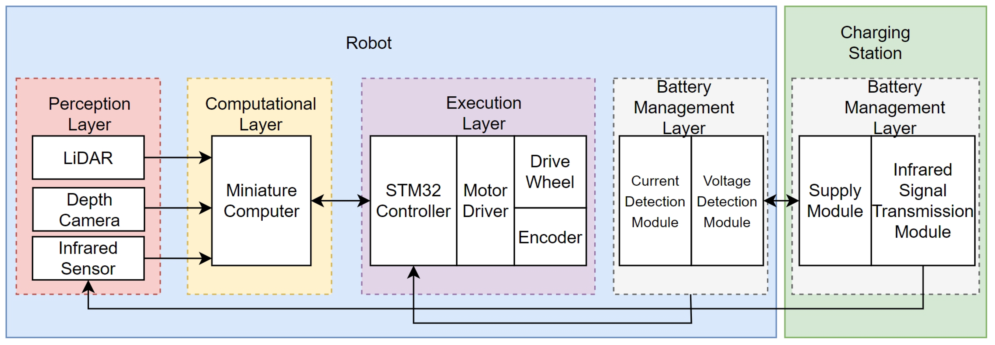
2.1. Hardware Components of the Multi-Sensor Fusion-Based Autonomous Recharging System
2.2. Software Components of Multi-Sensor Fusion for Automatic Recharging Systems
3. Multi-Sensor-Based Remote Autonomous Navigation and Close-Range Docking Localization
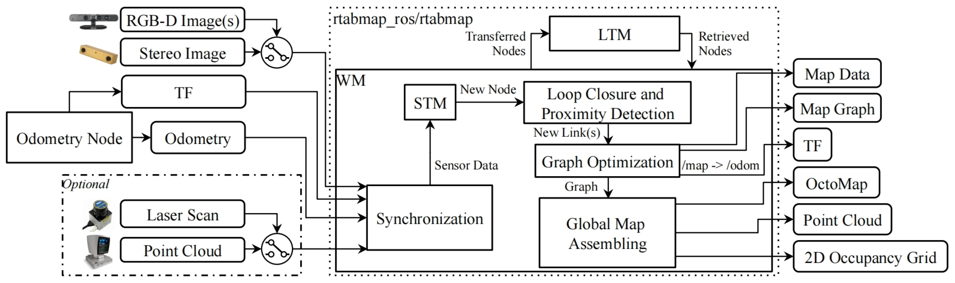
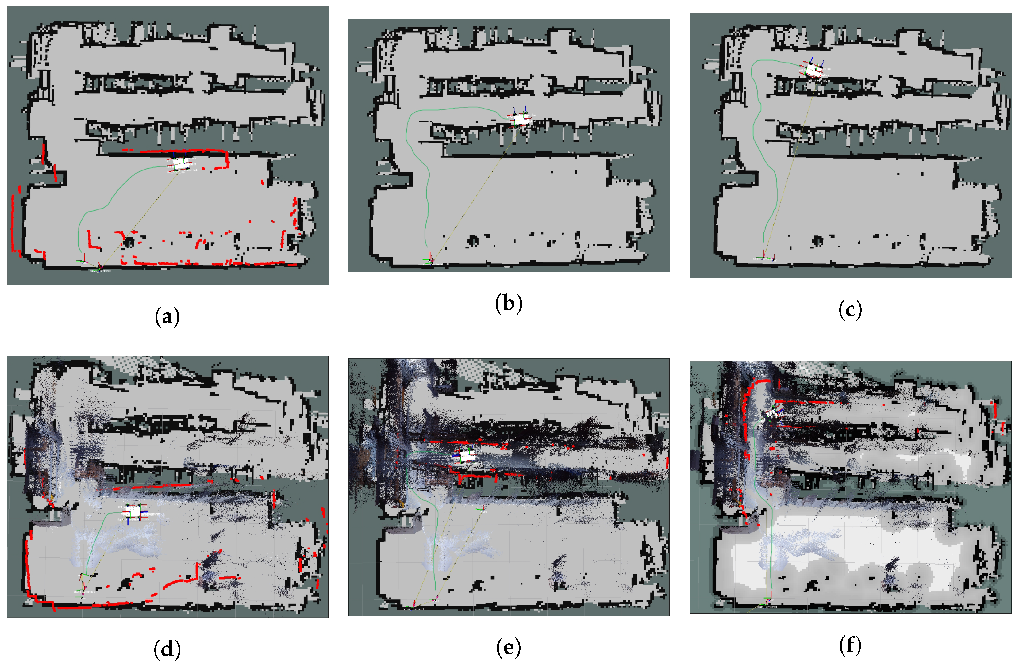
3.1. Remote Autonomous Navigation Based on LiDAR, Vision, and IMU Fusion
- Localization point acquisition: The RTAB-Map uses SURF to extract visual word features. The feature set of the image at time t is referred to as the image signature . The current localization point is created using the signature and time t.
- Localization point weight update: The similarity s between the current localization point and the last localization point in short-term memory is computed by comparing the number of matching word pairs between signatures and the total number of words in the signatures. This similarity s is used to determine the new weight of the localization point . The formula for is:where represents the number of matches and and denote the total number of words in signatures and , respectively.
- Bayesian filter update: The Bayesian filter calculates the likelihood of forming a loop between the current localization point and points within the working memory (WM). represents all loop closure hypotheses at time t, where indicates that forms a loop closure with an already visited localization point. The posterior probability distribution is computed as follows:where is a normalization factor, is the sequence of localization points, and represents the time index of the most recent localization point stored in WM.
- Loop closure hypothesis selection: When is below a set threshold, the loop closure hypothesis with the highest probability in the transition model is accepted. A loop closure link is established between the new and old localization points, and the weight of the localization points is updated.
- Localization point retrieval: To make full use of high-weight localization points, after a loop closure is detected, if the probability of forming a loop with adjacent localization points is highest, the localization point is moved from LTM back to WM. The words in the dictionary are updated for future loop closure detection.
- Localization point transfer: To meet the real-time requirements of the RTAB-Map, if the localization matching time exceeds a fixed maximum value , it indicates that these localization points are unlikely to form a loop closure. They are transferred from WM to LTM and will no longer participate in loop closure detection, reducing unnecessary time loss in localization.
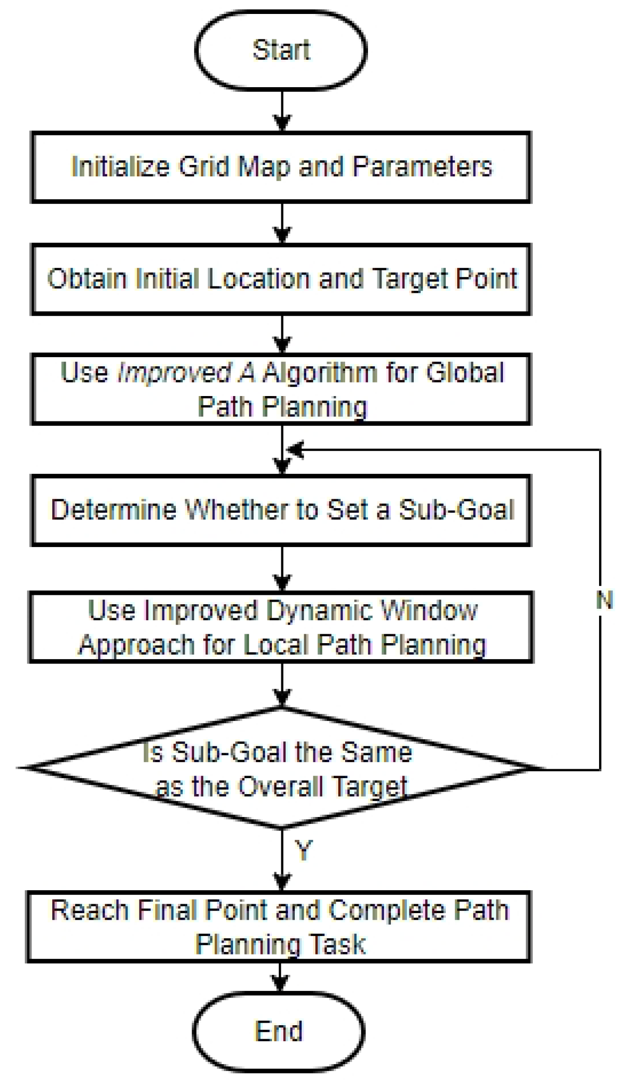
3.2. Automatic Recharging Path Planning Algorithm
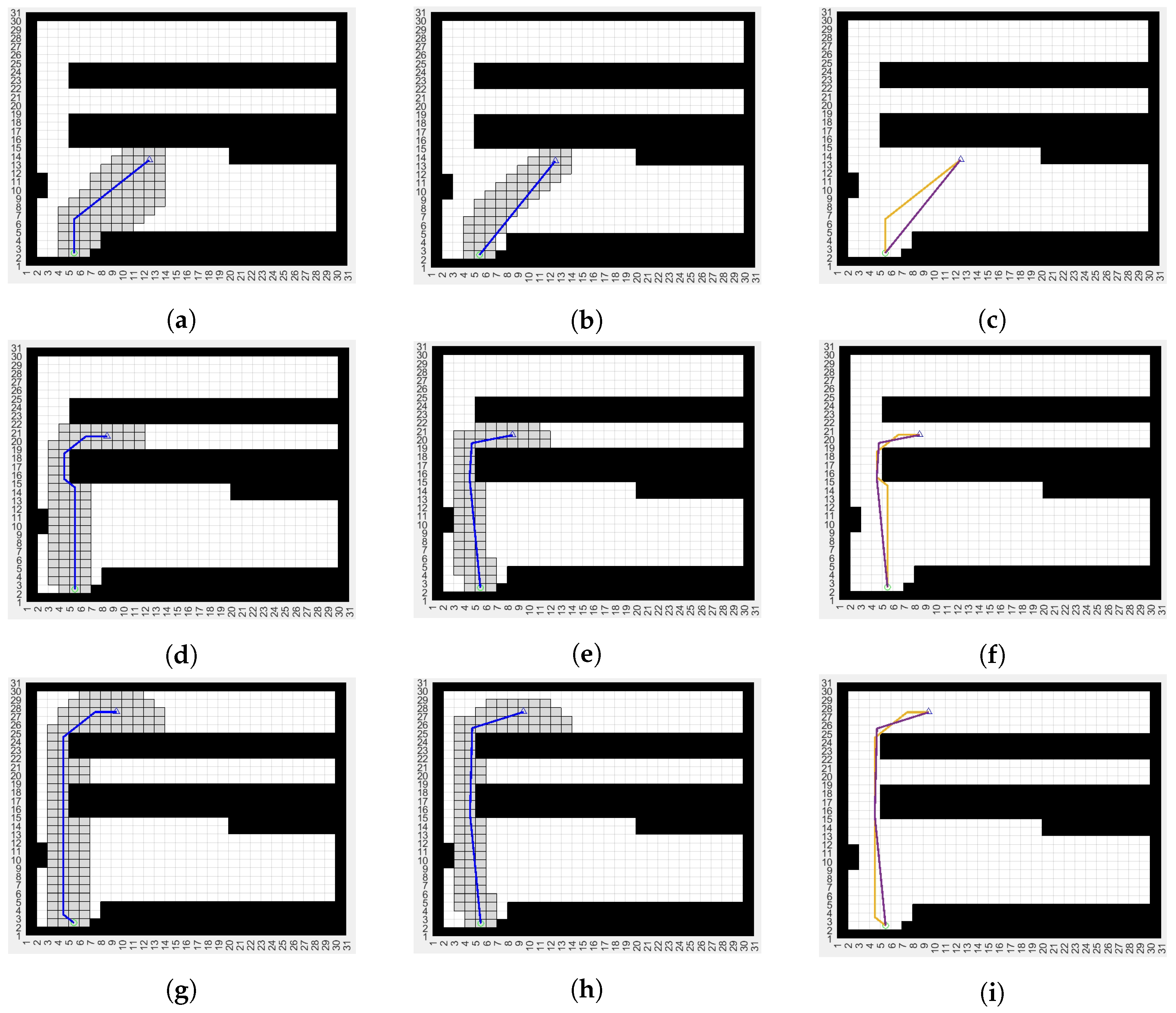
3.2.1. Improved A* Algorithm
- Traverse all nodes in the path sequentially. If the current node and the two adjacent nodes are collinear, remove the current node.
- After removing redundant points on the same straight line, let the nodes in the path be . Connect and . If the distance between the line segment and obstacles is greater than the set safety distance, then connect and until the distance between and obstacles is less than the set safety distance. Then, connect and , remove the intermediate nodes, and repeat the above operation starting from until all nodes in the path have been traversed.
3.2.2. Improved Dynamic Window Algorithm
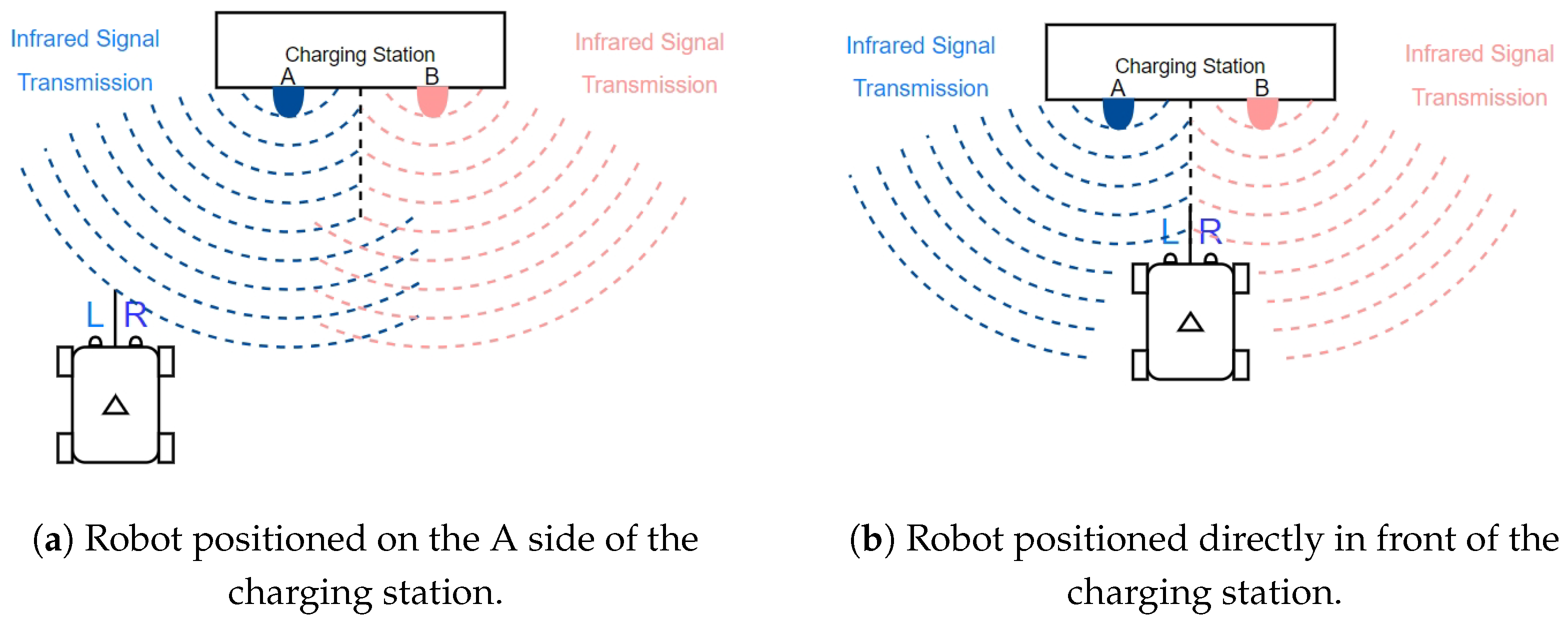
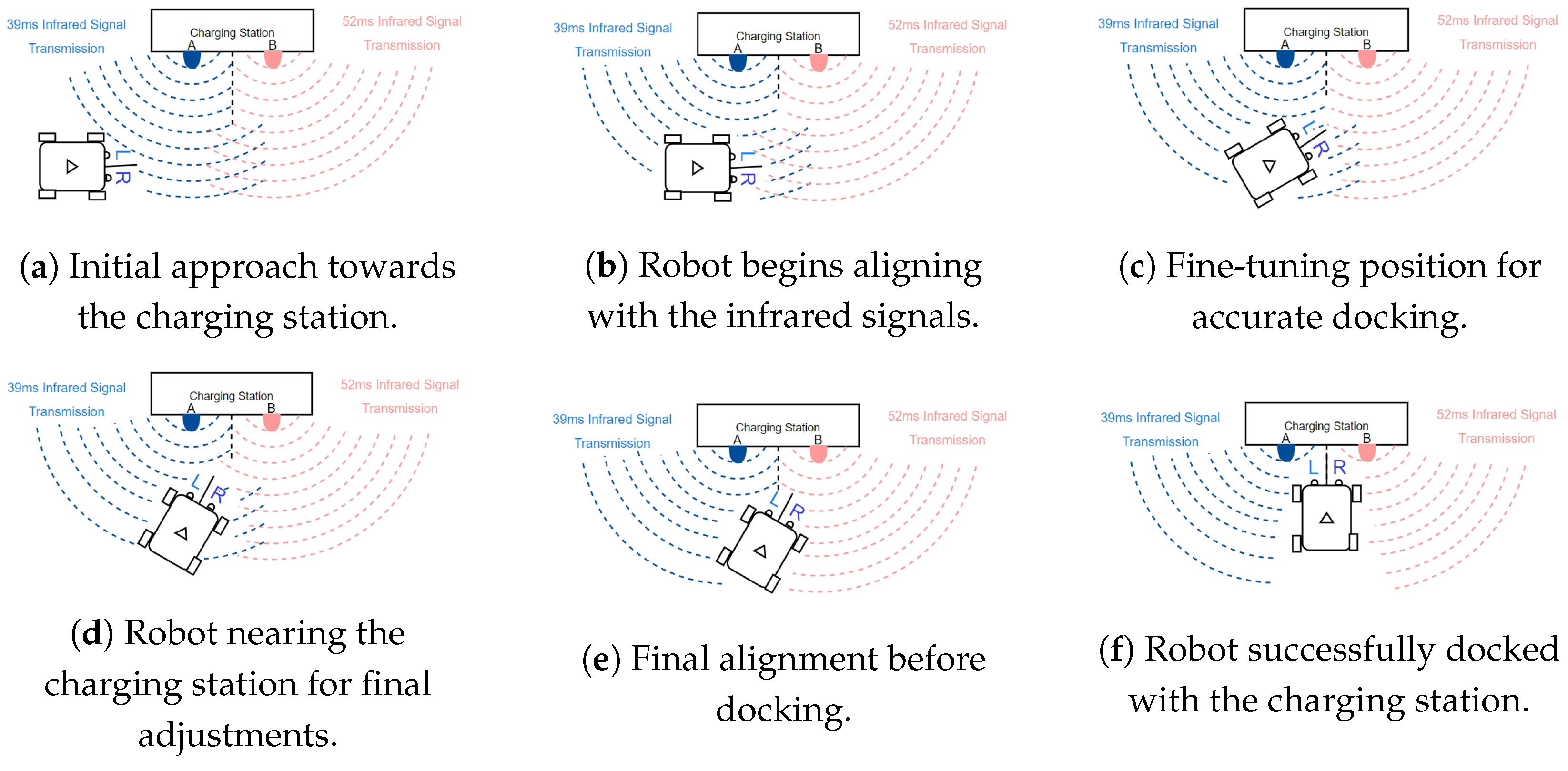
3.3. Proximity Docking Localization Based on Infrared Sensors
4. Experiments
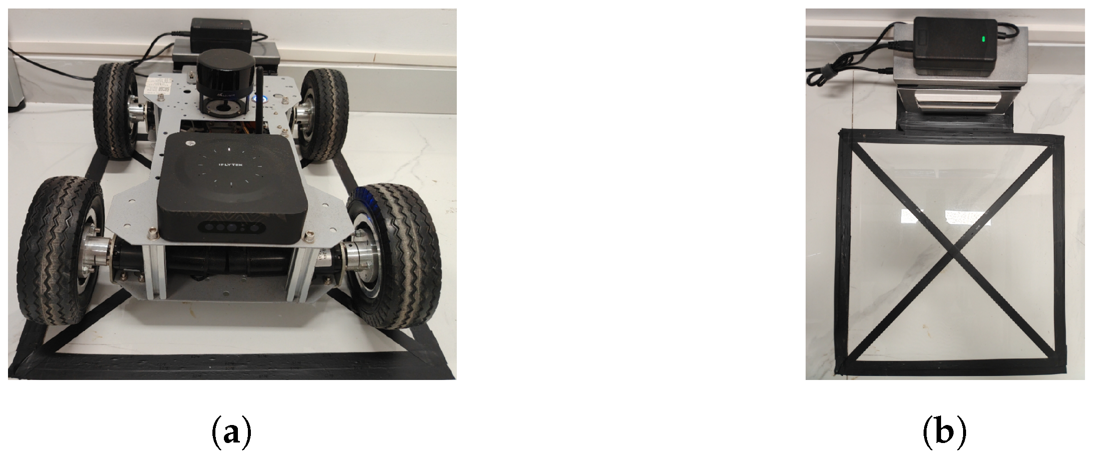
4.1. Hardware
4.2. Infrared Docking
5. Conclusions
Author Contributions
Funding
Institutional Review Board Statement
Informed Consent Statement
Data Availability Statement
Conflicts of Interest
References
- Su, K.L.; Liao, Y.L.; Lin, S.P.; Lin, S.F. An interactive auto-recharging system for mobile robots. Int. J. Autom. Smart Technol. 2014, 4, 43–53. [Google Scholar] [CrossRef]
- Moshayedi, A.J.; Jinsong, L.; Liao, L. AGV (automated guided vehicle) robot: Mission and obstacles in design and performance. J. Simul. Anal. Novel Technol. Mech. Eng. 2019, 12, 5–18. [Google Scholar]
- Song, G.; Wang, H.; Zhang, J.; Meng, T. Automatic docking system for recharging home surveillance robots. IEEE Trans. Consum. Electron. 2011, 57, 428–435. [Google Scholar] [CrossRef]
- Hao, B.; Du, H.; Dai, X.; Liang, H. Automatic recharging path planning for cleaning robots. Mobile Inf. Syst. 2021, 2021, 5558096. [Google Scholar] [CrossRef]
- Meena, M.; Thilagavathi, P. Automatic docking system with recharging and battery replacement for surveillance robot. Int. J. Electron. Comput. Sci. Eng. 2012, 1148–1154. [Google Scholar]
- Niu, Y.; Habeeb, F.A.; Mansoor, M.S.G.; Gheni, H.M.; Ahmed, S.R.; Radhi, A.D. A photovoltaic electric vehicle automatic charging and monitoring system. In Proceedings of the 2022 International Symposium on Multidisciplinary Studies and Innovative Technologies (ISMSIT), Ankara, Turkey, 20–22 October 2022; pp. 241–246. [Google Scholar]
- Rao, M.V.S.; Shivakumar, M. IR based auto-recharging system for autonomous mobile robot. J. Robot. Control (JRC) 2021, 2, 244–251. [Google Scholar] [CrossRef]
- Ding, G.; Lu, H.; Bai, J.; Qin, X. Development of a high precision UWB/vision-based AGV and control system. In Proceedings of the 2020 5th International Conference on Control and Robotics Engineering (ICCRE), Osaka, Japan, 24–26 April 2020; pp. 99–103. [Google Scholar]
- Liu, Y.; Piao, Y.; Zhang, L. Research on the positioning of AGV based on Lidar. J. Phys. Conf. Ser. 2021, 1920, 012087. [Google Scholar] [CrossRef]
- Yan, L.; Dai, J.; Tan, J.; Liu, H.; Chen, C. Global fine registration of point cloud in LiDAR SLAM based on pose graph. J. Geod. Geoinf. Sci. 2020, 3, 26–35. [Google Scholar]
- Gao, H.; Ma, Z.; Zhao, Y. A fusion approach for mobile robot path planning based on improved A* algorithm and adaptive dynamic window approach. In Proceedings of the 2021 IEEE 4th International Conference on Electronics Technology (ICET), Chengdu, China, 7–10 May 2021; pp. 882–886. [Google Scholar]
- Tang, G.; Tang, C.; Claramunt, C.; Hu, X.; Zhou, P. Geometric A-star algorithm: An improved A-star algorithm for AGV path planning in a port environment. IEEE Access 2021, 9, 59196–59210. [Google Scholar] [CrossRef]
- Sun, Y.; Zhao, X.; Yu, Y. Research on a random route-planning method based on the fusion of the A* algorithm and dynamic window method. Electronics 2022, 11, 2683. [Google Scholar] [CrossRef]
- Zhou, S.; Cheng, G.; Meng, Q.; Lin, H.; Du, Z.; Wang, F. Development of multi-sensor information fusion and AGV navigation system. In Proceedings of the 2020 IEEE 4th Information Technology, Networking, Electronic and Automation Control Conference (ITNEC), Chongqing, China, 12–14 June 2020; pp. 2043–2046. [Google Scholar]
- Zhang, J.; Singh, S. Laser–visual–inertial odometry and mapping with high robustness and low drift. J. Field Robot. 2018, 35, 1242–1264. [Google Scholar] [CrossRef]
- Jiang, Y.; Leach, M.; Yu, L.; Sun, J. Mapping, navigation, dynamic collision avoidance and tracking with LiDAR and vision fusion for AGV systems. In Proceedings of the 2023 28th International Conference on Automation and Computing (ICAC), Birmingham, UK, 30 August–1 September 2023; pp. 1–6. [Google Scholar]
- Dai, Z.; Guan, Z.; Chen, Q.; Xu, Y.; Sun, F. Enhanced object detection in autonomous vehicles through LiDAR—Camera sensor fusion. World Electr. Vehicle J. 2024, 15, 297. [Google Scholar] [CrossRef]
- Labbé, M.; Michaud, F. RTAB-Map as an open-source lidar and visual simultaneous localization and mapping library for large-scale and long-term online operation. J. Field Robot. 2019, 36, 416–446. [Google Scholar] [CrossRef]
- Das, S. Simultaneous localization and mapping (SLAM) using RTAB-MAP. arXiv 2018, arXiv:1809.02989. [Google Scholar]
- Gomez-Ojeda, R.; Moreno, F.A.; Zuniga-Noël, D.; Scaramuzza, D.; Gonzalez-Jimenez, J. PL-SLAM: A stereo SLAM system through the combination of points and line segments. IEEE Trans. Robot. 2019, 35, 734–746. [Google Scholar] [CrossRef]


| Metric | Traditional A* (Experiment 1) | Traditional A* (Experiment 2) | Traditional A* (Experiment 3) | Improved A* (Experiment 1) | Improved A* (Experiment 2) | Improved A* (Experiment 3) |
|---|---|---|---|---|---|---|
| Planning time (s) | 0.020610 | 0.007665 | 0.004626 | 0.027963 | 0.020292 | 0.014692 |
| Turn angle | 45.0000 | 180.0000 | 135.0000 | 0.0000 | 80.3964 | 72.6313 |
| Turn count | 1.0000 | 4.0000 | 3.0000 | 0.0000 | 2.0000 | 2.0000 |
| Path length | 13.8995 | 21.2426 | 28.6569 | 13.0384 | 21.0105 | 28.2904 |
| Node count | 81 | 84 | 123 | 53 | 73 | 100 |
| Position | Sensor | S1 | S2 | S3 | S4 | S5 | S6 | S7 | S8 |
|---|---|---|---|---|---|---|---|---|---|
| L | A | 1 | 1 | 1 | 1 | 1 | 1 | 1 | 1 |
| B | 1 | 1 | 1 | 1 | 0 | 0 | 0 | 0 | |
| R | A | 1 | 1 | 0 | 0 | 1 | 1 | 0 | 0 |
| B | 1 | 0 | 1 | 0 | 1 | 0 | 1 | 0 | |
| Control Action | Back | / | Reverse | Reverse | Forward | Forward | Back | Back | |
| X-axis (m/s) | −0.1 | / | 0 | 0 | 0 | −0.1 | −0.1 | −0.1 | |
| Z-axis (rad/s) | 0 | / | 0.1 | 0.1 | −0.1 | −0.1 | 0 | 0 | |
| Test Variable | Infrared Only | LiDAR Only | Vision Only | LiDAR + Vision | LiDAR + Vision + Infrared |
|---|---|---|---|---|---|
| Docking success rate (%) | 50 | 70 | 50 | 80 | 95 |
| Average docking time (s) | 60 | 45 | 55 | 35 | 25 |
| Docking error (cm) | 15 | 10 | N/A | 8 | 3 |
| Obstacle adaptability | Poor | Medium | Poor | Excellent | Excellent |
| Lighting condition adaptability | Excellent | Excellent | Poor | Good | Excellent |
| Path planning distance (m) | N/A | 20 | N/A | 20 | 19 |
| Time to reach destination (s) | N/A | 45 | N/A | 40 | 35 |
Disclaimer/Publisher’s Note: The statements, opinions and data contained in all publications are solely those of the individual author(s) and contributor(s) and not of MDPI and/or the editor(s). MDPI and/or the editor(s) disclaim responsibility for any injury to people or property resulting from any ideas, methods, instructions or products referred to in the content. |
© 2024 by the authors. Licensee MDPI, Basel, Switzerland. This article is an open access article distributed under the terms and conditions of the Creative Commons Attribution (CC BY) license (https://creativecommons.org/licenses/by/4.0/).
Share and Cite
Xue, Y.; Wang, L.; Li, L. Research on Automatic Recharging Technology for Automated Guided Vehicles Based on Multi-Sensor Fusion. Appl. Sci. 2024, 14, 8606. https://doi.org/10.3390/app14198606
Xue Y, Wang L, Li L. Research on Automatic Recharging Technology for Automated Guided Vehicles Based on Multi-Sensor Fusion. Applied Sciences. 2024; 14(19):8606. https://doi.org/10.3390/app14198606
Chicago/Turabian StyleXue, Yuquan, Liming Wang, and Longmei Li. 2024. "Research on Automatic Recharging Technology for Automated Guided Vehicles Based on Multi-Sensor Fusion" Applied Sciences 14, no. 19: 8606. https://doi.org/10.3390/app14198606
APA StyleXue, Y., Wang, L., & Li, L. (2024). Research on Automatic Recharging Technology for Automated Guided Vehicles Based on Multi-Sensor Fusion. Applied Sciences, 14(19), 8606. https://doi.org/10.3390/app14198606