Abstract
The mechanics and motion behavior of granular materials affect the production and life of human beings. In order to study the influence of the sliding friction coefficients corresponding to different contact types in the block discrete element method on the simulation results, this study established a block discrete element model to analyze a slope example based on the test method. The example was a homogeneous soil slope that did not consider water. The correctness of the models was verified by establishing the block discrete element slope model and comparing it with the known finite element method (FEM) model in terms of the maximum shear strain. Then, the sliding friction coefficient algorithm was embedded into the discrete element slope model for comparative analysis. The results show that in the calculations in the block discrete element method, the sliding friction coefficients of different contact types are different. Different sliding friction coefficients should be set based on different contact types to improve the accuracy of the simulation. Because the block discrete element model needs to preset the landslide surface of the slope, the displacement at the edge of the landslide surface is slightly different. The discrete element method (DEM) model was also compared with the block element model, and the results show that the DEM model is more stable.
1. Introduction
The mechanics and motion behavior of granular materials affect the production and life of human beings [1,2,3,4,5]. For example, landslides [6,7], avalanches [8,9,10], debris flow [11,12], and sand liquefaction [13,14,15] caused by earthquakes and other disasters [16,17,18,19] have a profound impact on the safety of human life and property [20,21].
Rock and soil are both granular materials. From a microscopic point of view, they are both composed of granular materials. These granular materials exist independently, and there is no force when contact does not occur [22,23]. Granular material is very different from a continuous medium. The biggest difference is that the granular matter flows easily under the action of external force, and it is difficult to maintain a static shape. At the same time, the flow properties of granular materials are also very different from those of fluids. When granular materials flow or are subjected to pressure, their physical parameters change [24]. For geotechnical engineering, because the discrete element method (DEM) can truly represent the geometric characteristics of rock and soil and efficiently simulate the processes of joints [25,26,27,28,29], slopes [30,31,32,33], landslides [34,35,36], and seepage [37,38,39], it has become an indispensable tool for analyzing and dealing with geotechnical engineering problems [40,41,42].
The discrete element method, which was proposed by Cundall and Strack [43,44,45] in the 1970s, is an effective tool to simulate the mechanical behavior of granular materials. According to the difference in the basic shape elements used in the modeling of the discrete element method, the elements can be divided into two categories: particle elements and block elements. That is, the discrete element method can be divided into the particle discrete element method and the block discrete element method [46]. The research and application of regularly shaped elements in the DEM, such as particle elements, are very extensive in the field of geotechnical engineering. However, there are still many areas worthy of attention in the study of irregularly shaped elements [47].
A clump Is one of the terms used to describe irregularly shaped particles. Its core is formed of an arbitrary geometry through multiple circle or sphere elements [48,49]. Favier [50] described the process of solving the contact problem of the cluster elements widely used in discrete element numerical simulation. Zhao [51] compared the shear mechanical behavior of the cluster and sphere elements in an undrained triaxial test and found that the cluster element can greatly improve the shear strength. The irregularity of the cluster element shape can improve the residual shear strength. Brzeziński [52] proposed a crushing algorithm for cluster elements, which can calculate the stress state of each sub-element, usually called a pebble, and applied it in Yade software. Grabowski [53] used asymmetric cluster and sphere elements to simulate the mechanical behavior of sand in a direct shear test. Li [54], Lu [55], Ferellec [56], and other scholars also studied the influence of the radius and number of sub-elements (pebbles) on the simulation results by comparing the numerical simulation experiments of cluster and sphere elements.
Polygonal or polyhedral elements are also often used to describe irregular particles [57], but there are some problems in their contact discovery and time-consuming calculation. Liu [57] developed polyhedron–polyhedron and sphere–polyhedron contact discovery algorithms based on energy conservation, proposed a polyhedron–boundary contact discovery algorithm [58], and developed the CoSim-DEM discrete element framework program. Descantes [59] proposed an improved Gilbert–Johnson–Keerthi Distance Algorithm (GJK-TD) based on the GJK contact detection algorithm and verified it using a frictionless polyhedron accumulation test and a friction polyhedron rolling test. In order to simulate the fracture process of rock and other geotechnical materials, Cui [60] proposed a cohesive fracture model and verified it using the Brazilian splitting test and uniaxial compression test. Feng [61], Fraige [62], Nezami [63], and other scholars have improved the two-dimensional polygon elements and three-dimensional polyhedron elements to improve their calculation accuracy.
Based on the sliding friction coefficient test of different elements of the discrete element method in the study by Liu [64], the block discrete element numerical simulation of a slope was carried out. By comparing the known FEM simulation results [65] with the block discrete element simulation results, the correctness of the block discrete element model was verified. By comparing the model embedded with the sliding friction coefficient determined by contact types and the FEM model, it was found that the sliding friction coefficients of different contact types should be set differently in the block discrete element numerical simulation. Different sliding friction coefficients were set based on different contact types to improve the accuracy of the discrete element simulation.
2. Experimental Method
In order to study the influence of the sliding friction coefficients of different contact types in block discrete elements on numerical simulation, this study featured further research based on previous experiments [64]. The research object of this study was samples embedded with polyhedrons made of cement. The polyhedron size was a cube with a side length of 40.24 mm, and the samples were cast using a silica gel reverse mold. The names of the samples, the average size of the cube, and the number of embedded cubes are shown in Table 1. In Table 1, P denotes the polyhedron, and the subscripts p, e, and f denote point contact, edge contact, and face contact. Two groups were made of various samples, and the sliding friction coefficient under different contact types was measured by contact between the samples. In the block discrete element method, the types of contact between the elements are categorized as point–point contact, point–edge contact, point–surface contact, edge–edge contact, edge–surface contact, and surface–surface contact. For convenience in description and recording, test results were documented using combinations of “point”, “edge”, and “surface”. The test results are shown in Table 2. Specific information about the experiment can be found in the study by Liu [64].

Table 1.
The labels, average size, amount, and explanations for the experiment.
Table 2.
The sliding friction coefficients between the polyhedrons.
3. Simulated Model
In order to study the influence of the sliding friction coefficients corresponding to different contact types in the block discrete element method on the simulation results, this study used the block discrete element method to analyze a sand slope example [65] based on the experiment method [46]. The slope was homogeneous without considering other factors, such as the water content. The correctness of the block discrete element slope model was verified by comparing it with the known FEM model, and then the sliding friction coefficient algorithm was embedded into the discrete element slope model for comparative analysis.
The slope comprises two sections: the lower section is 45° and the upper section is 26.7°. The slope geometry is shown in Figure 1. The material parameters of the slope are shown in Table 3.
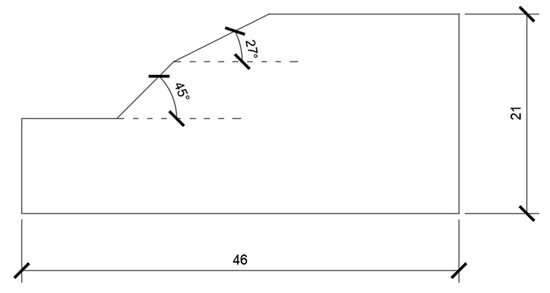
Figure 1.
The geometry of the slope.
Table 3.
The parameters of the slope model.
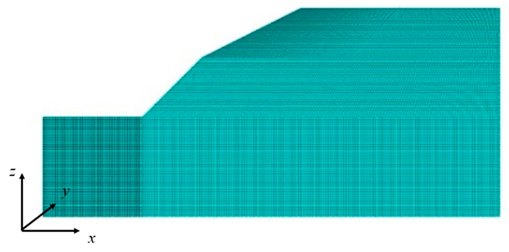
Based on the conditions given by Cheng, the model was established as shown in Figure 2. Because the length in the y direction is just a unit, and the deformation in the y direction is limited, it can be simplified to a plane strain problem.
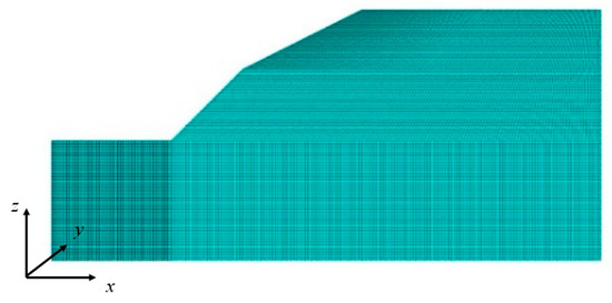
Figure 2.
The slope model.
According to the maximum shear strain range based on Figure 3a and the displacement area based on Figure 3b of the FEM model, the displacement region points outward from the slope, a slightly larger sliding range was preset in the block discrete element model, and the sliding range in the simulation results was taken as the main research object in the block discrete element model. Because the calculation stability of the block discrete element software depends on the element size and material parameters of each block, the landslide surface to the boundary was divided into six parts, as shown in Figure 4a. The landslide range is in the green area, which uses a Voronoi grid to divide the polygonal elements. The parameters of the slope model are shown in Table 1. The sliding friction coefficient of this paper was embedded in the model after verification.
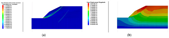
Figure 3.
The result of the slope mode: (a) the shear strain of the model; (b) the displacement of the model.
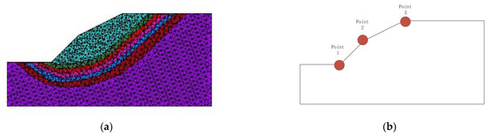
Figure 4.
The block discrete element model and the measuring points: (a) The block discrete element model; (b) The measuring points of the modal.
Three measuring points were set up on the model, and the positions are shown in Figure 4b. Each measuring point recorded the horizontal and vertical displacements of each time step.
4. Results and Discussions
The correctness of the original block discrete element slope model was verified by comparing the maximum shear strain with that of the known FEM model. The maximum shear strains are 3.17 × 10⁻¹ and 1.08 × 10⁻², respectively, which are very close, as shown in Figures 3a and 9a, and the maximum shear strain occurred near the edge of the landslide surface, indicating that the original block discrete element model was established correctly. Because of the difference between the block discrete element method and FEM, the calculated maximum shear strain is slightly different, but the calculation results are within a reasonable range.
In order to verify that the sliding friction coefficient determined by the test method was embedded in the block discrete element model, the original block discrete element model that calculates the default sliding friction coefficient was compared and verified. A total of 21,000 time steps were calculated, and the maximum shear strain distribution contours at the output of 5000, 10,000, 15,000, 20,000, and the end of the simulation calculation were compared, as shown in Figure 5, Figure 6, Figure 7, Figure 8 and Figure 9, respectively.
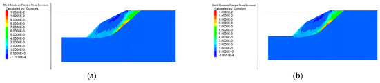
Figure 5.
The maximum shear strain distribution at the 5000th time step: (a) the original block discrete element model; (b) the block discrete element model embedded with the sliding friction coefficient.
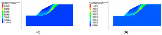
Figure 6.
The maximum shear strain distribution at the 10,000th time step: (a) the original block discrete element model; (b) the block discrete element model embedded with the sliding friction coefficient.
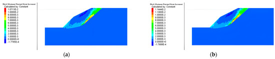
Figure 7.
The maximum shear strain distribution at the 15,000th time step: (a) the original block discrete element model; (b) the block discrete element model embedded with the sliding friction coefficient.
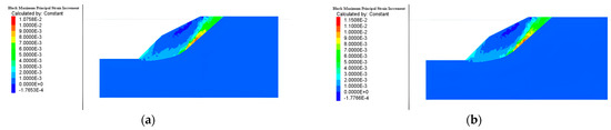
Figure 8.
The maximum shear strain distribution at the 20,000th time step: (a) the original block discrete element model; (b) the block discrete element model embedded with the sliding friction coefficient.

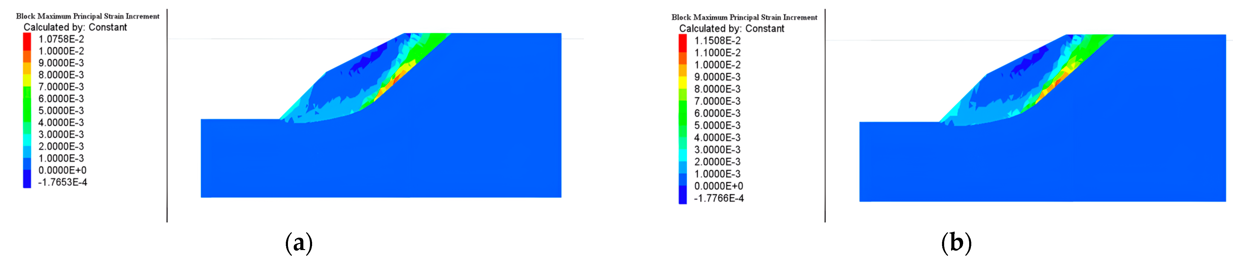
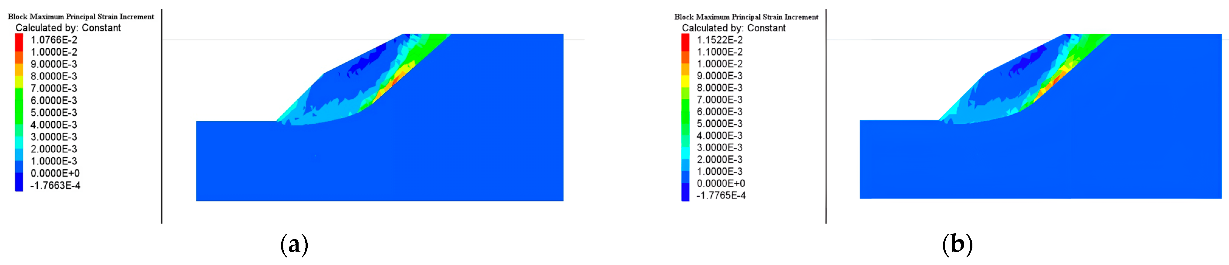
Figure 9.
The maximum shear strain distribution at the final time step: (a) the original block discrete element model; (b) the block discrete element model embedded with the sliding friction coefficient.
Comparing the original block discrete element slope model and the modified model embedded with the sliding friction coefficient in Figure 5, Figure 6, Figure 7, Figure 8 and Figure 9, the maximum shear strain is different at each time step, indicating that the sliding friction coefficient determined by the experiment method was successfully embedded and had an impact on the calculation results. Because the sliding friction coefficient between blocks determined by the experiment method is slightly smaller than the default value of the model, the maximum shear strain of the modified model embedded with the sliding friction coefficient is slightly larger than that of the original slope model. However, the calculation result is within a reasonable range because the interpolation of the maximum shear strain is only 7.56 × 10⁻⁴.
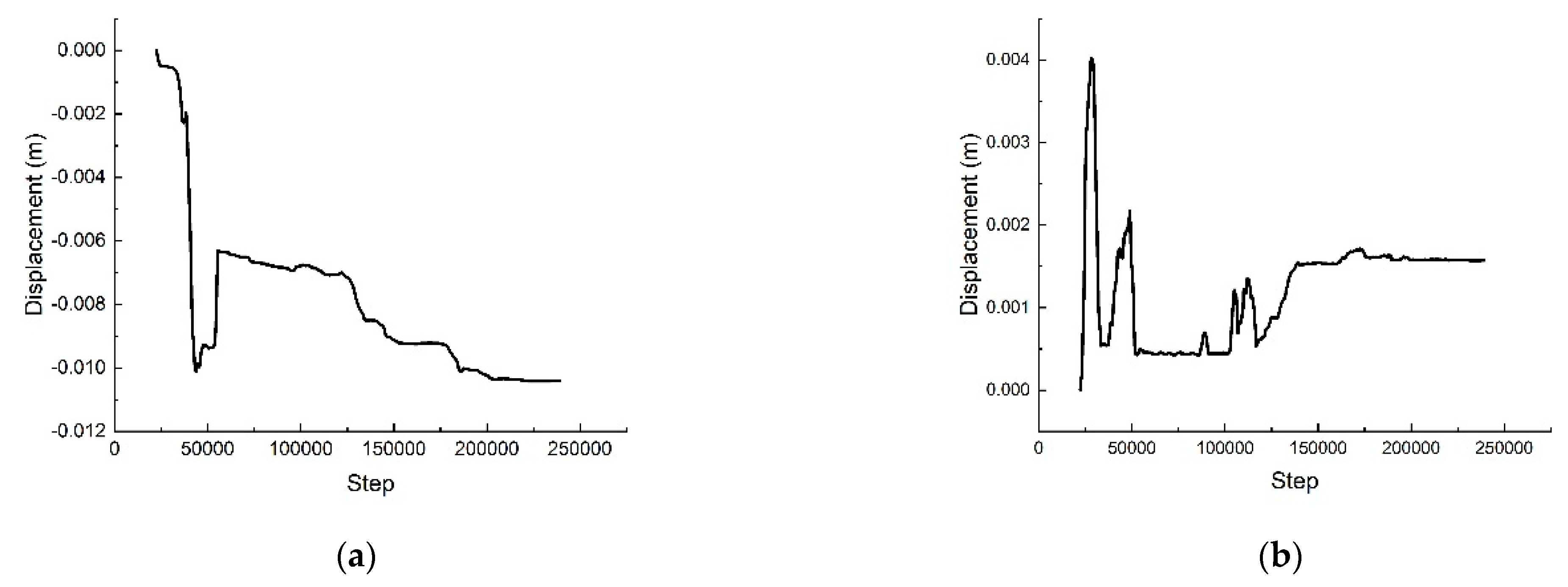
According to the position of each measuring point in Figure 4b, the change trend of the displacement of each measuring point in the modified model with the sliding friction coefficient was drawn, and the change trend of the displacement of each measuring point in the FEM model was drawn too. The horizontal and vertical displacements of each measuring point are shown in Figure 10, Figure 11, Figure 12, Figure 13, Figure 14 and Figure 15. Since the displacement changes at different monitoring points vary significantly based on different analysis methods (whether it is DEM, FEM, or block discrete element methods), with some very small and others so big, unifying the Y-axis would result in some displacement change curves appearing with very large amplitudes, while others would have very small amplitudes. As this section primarily compares the variation trends of the two methods at each measurement point and the final displacement values, this study did not use a unified Y-axis representation. The subsequent discussion comparing the displacements of the DEM and block discrete element methods will not be reiterated. According to the displacement diagram of each measuring point, the following conclusions can be illuminated:
- (1)
- The trend of the horizontal displacement of each measuring point is basically the same as the development of time. The displacement of measuring point 1 is negative in a very short time, then rises rapidly and finally stabilizes. Measuring points 2 and 3 both show rapid stability after the development of displacement;
- (2)
- The trend of vertical displacement of each measuring point is basically the same at any time, and the displacement develops rapidly and then stabilizes rapidly;
- (3)
- Table 4 shows the displacements calculated using different methods for sliding friction coefficients under the same computational theory (block discrete element method). When comparing the horizontal displacement and vertical displacement of each measuring point, as shown in Table 4, there is little difference in the horizontal displacement of measuring point 1 and the vertical displacement of measuring point 3. The results are mainly because the block discrete element model needs to set a certain landslide surface in advance. In block discrete element models, due to reasons such as the geometric shape of the elements, contact methods, contact theories, and contact detection, elements can easily become stuck and lead to erroneous conclusions during stability analysis if sliding surfaces are not preset. Therefore, in slope stability analysis, sliding surfaces are typically preset. Measuring point 1 is located at the foot of the slope, and measuring point 3 is located at the shoulder of the slope. The deformation of the two measuring points cannot be fully developed due to the factors of the preset landslide surface and the assumptions of the DEM that the element is rigid. However, the displacements of the two measuring points in other directions are very similar, and measuring point 2 is basically the same, which proves the correctness of the model again.

Figure 10.
The horizontal displacement of point 1: (a) the block discrete element model embedded with the sliding friction coefficient; (b) the FEM model.
Figure 10.
The horizontal displacement of point 1: (a) the block discrete element model embedded with the sliding friction coefficient; (b) the FEM model.
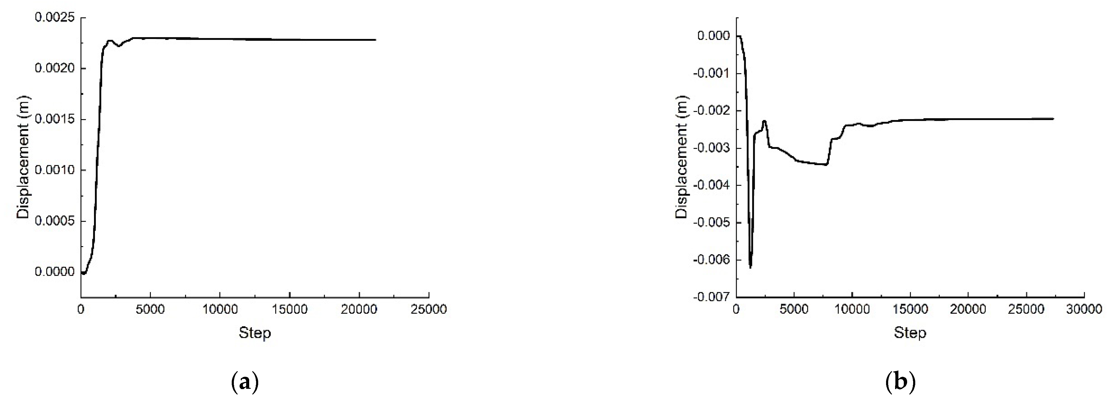
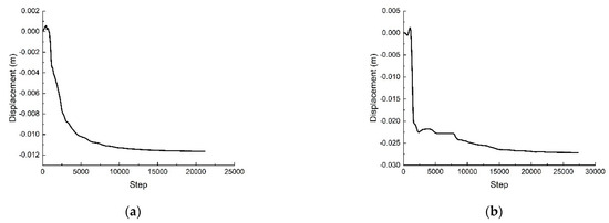
Figure 11.
The vertical displacement of point 1: (a) the block discrete element model embedded with the sliding friction coefficient; (b) the FEM model.
Figure 11.
The vertical displacement of point 1: (a) the block discrete element model embedded with the sliding friction coefficient; (b) the FEM model.
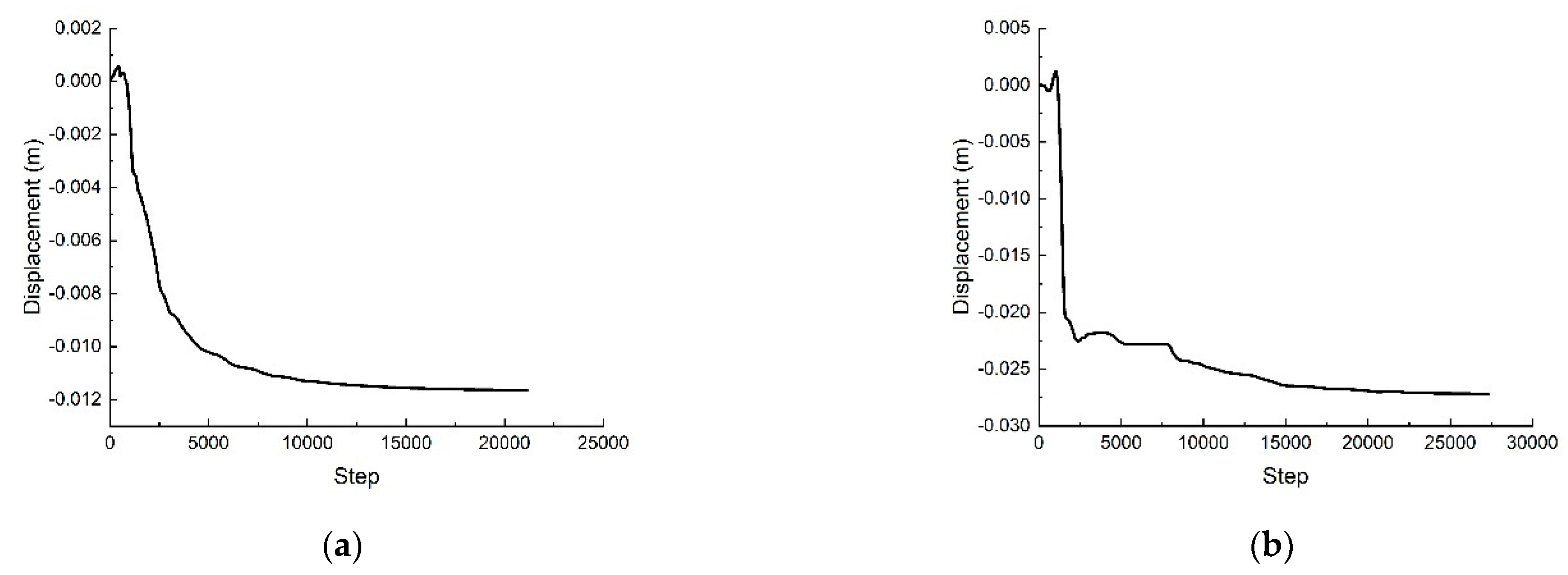
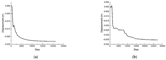
Figure 12.
The horizontal displacement of point 2: (a) the block discrete element model embedded with the sliding friction coefficient; (b) the FEM model.
Figure 12.
The horizontal displacement of point 2: (a) the block discrete element model embedded with the sliding friction coefficient; (b) the FEM model.
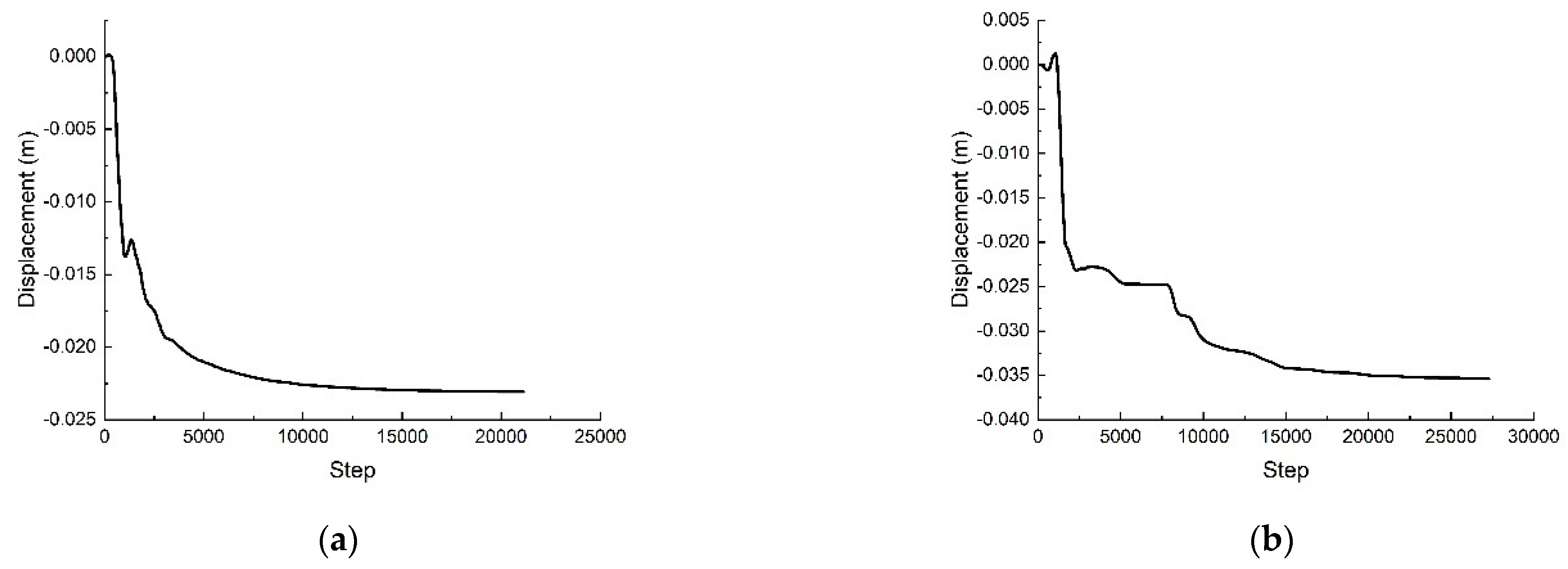
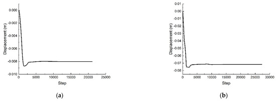
Figure 13.
The vertical displacement of point 2: (a) the block discrete element model embedded with the sliding friction coefficient; (b) the FEM model.
Figure 13.
The vertical displacement of point 2: (a) the block discrete element model embedded with the sliding friction coefficient; (b) the FEM model.

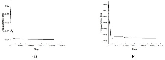
Figure 14.
The horizontal displacement of point 3: (a) the block discrete element model embedded with the sliding friction coefficient; (b) the FEM model.
Figure 14.
The horizontal displacement of point 3: (a) the block discrete element model embedded with the sliding friction coefficient; (b) the FEM model.
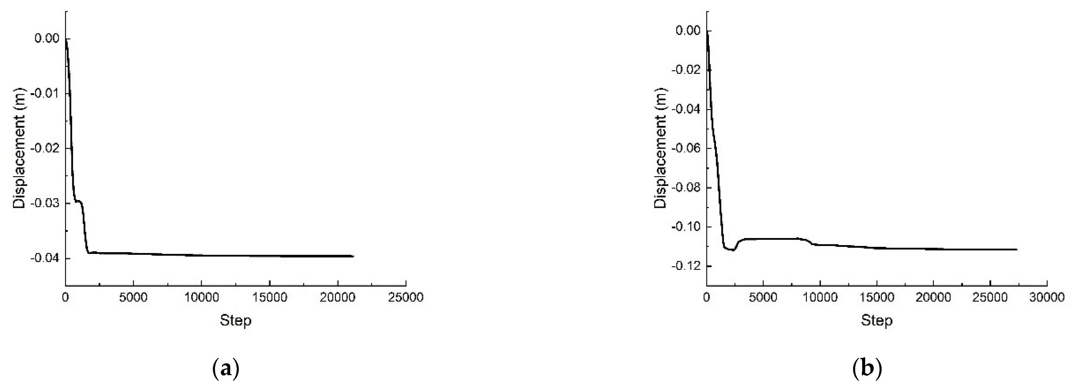

Figure 15.
The vertical displacement of point 3: (a) the block discrete element model embedded with the sliding friction coefficient; (b) the FEM model.
Figure 15.
The vertical displacement of point 3: (a) the block discrete element model embedded with the sliding friction coefficient; (b) the FEM model.
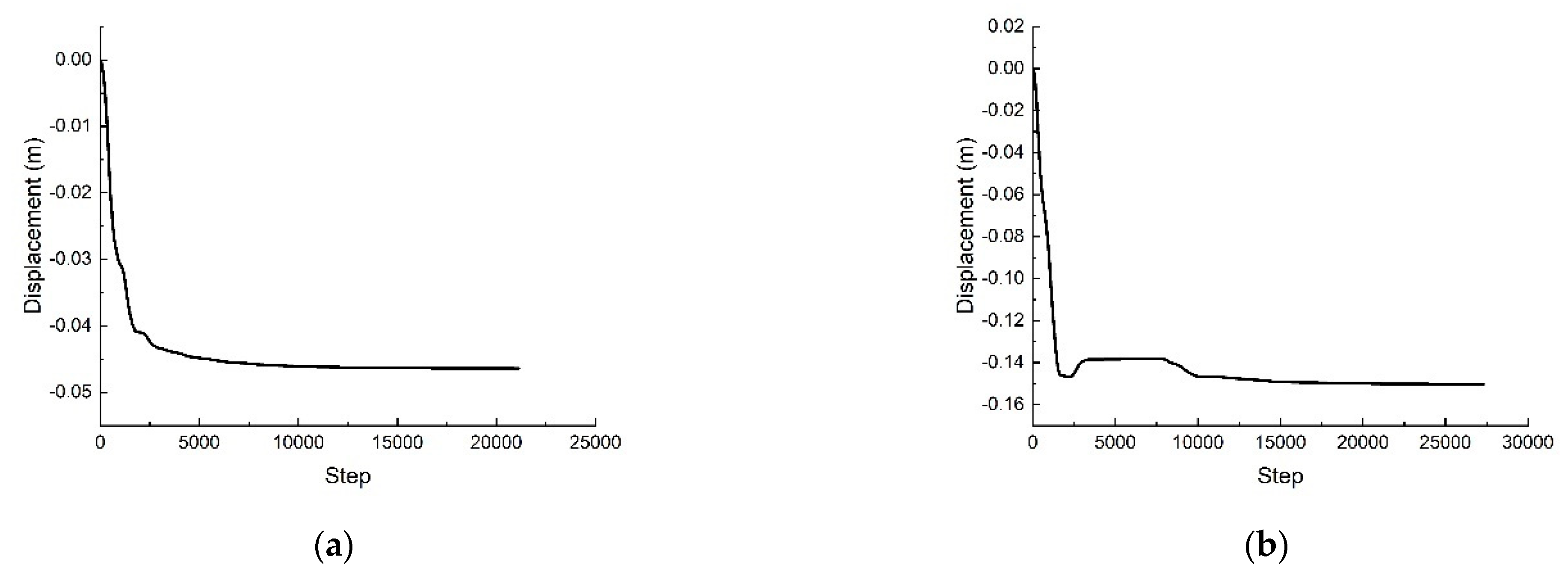
Table 4.
A comparison of the displacement values of the measuring points.
Table 4.
A comparison of the displacement values of the measuring points.
| Measuring Point | Original Model (cm) | Modified Model (cm) |
|---|---|---|
| Horizontal displacement of point 1 | 0.2 | −0.2 |
| Vertical displacement of point 1 | −0.8 | −7.2 |
| Horizontal displacement of point 2 | −1.1 | −2.6 |
| Vertical displacement of point 2 | −3.9 | −11.3 |
| Horizontal displacement of point 3 | −2.2 | −3.4 |
| Vertical displacement of point 3 | −4.5 | −15.2 |
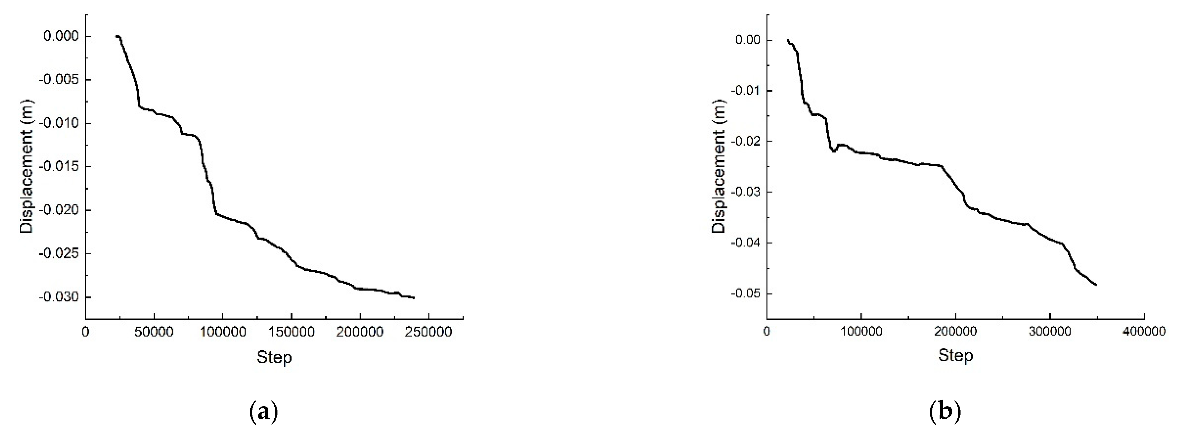
This study also established a discrete element method (DEM) model and a block discrete element model for comparison. The horizontal and vertical displacements of each measuring point are shown in Figure 16, Figure 17 and Figure 18. Comparing the displacements of each measuring point in the DEM model and the BDEM model reveals the following.
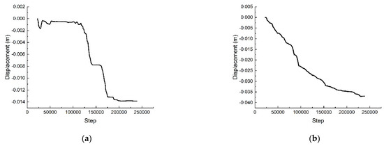
Figure 16.
The displacement of point 1 in the DEM model: (a) the horizontal displacement; (b) the vertical displacement.

Figure 17.
The displacement of point 2 in the DEM model: (a) the horizontal displacement; (b) the vertical displacement.
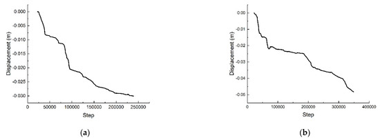
Figure 18.
The displacement of point 3 in the DEM model: (a) the horizontal displacement; (b) the vertical displacement.
The overall trends of displacement at each measuring point are similar. However, due to the gaps between the DEM elements, noticeable displacement fluctuations occur during movement. These fluctuations can be smoothed out to achieve a more consistent displacement–time curve by reducing the time step or decreasing the element size. However, such adjustments significantly increase the computation time; thus, these minor fluctuations may be disregarded. From a macroscopic perspective, these fluctuations represent negligible deformations.
The horizontal displacement at measuring point 1 in the DEM model differs slightly from that in the block discrete element model, yet the development trend at this point aligns closely between the DEM and FEM models. This suggests that the DEM model provides a more realistic simulation of slope behavior compared to the block discrete element model. Unlike the block discrete element model, which requires predefining the slip surface, the DEM model exhibits more comprehensive development.
5. Conclusions
In order to study the influence of the sliding friction coefficients corresponding to different contact types in the block discrete element method on the simulation results, the sliding friction coefficient algorithm was applied to a slope example based on the experiment method. The correctness of the block discrete element model was verified by comparing the maximum shear strain of the known FEM model with that of the block discrete element model before the sliding friction coefficient was embedded. Then, the displacement of each measuring point of the modified model was compared with the displacement of the measuring point of the known FEM model to verify the influence of the different contact types of the block discrete element on the sliding friction coefficient on the simulation results. The comparison results show the following:
- (1)
- The maximum shear strain cloud diagrams of the initial slope model and the embedded sliding friction coefficient model were compared and analyzed, indicating that the sliding friction coefficient affects the calculation of the block discrete element model. In calculating the block discrete element method, the sliding friction coefficients of the different contact types were different. Different sliding friction coefficients should be set for different contact types to improve the accuracy of the simulation;
- (2)
- When we compared and analyzed the trends of the horizontal and vertical displacements of each measuring point in the FEM model and block discrete element model with the sliding friction coefficient, they had the same change trend at each measuring point. The measuring points develop in the direction of deviation from the slope, showing a trend of gradual sliding;
- (3)
- Due to the different basic theories of the two methods, the FEM and discrete element methods, and because the block discrete element model needs to preset the landslide surface of the slope, the displacement at the edge of the landslide surface was slightly different. However, the total trends of the slope developments are the same. And the comparison between the DEM model and block discrete element model shows that the DEM model provides a more realistic simulation of slope behavior compared to the block discrete element model.
Author Contributions
P.L. contributed to the conceptualization, resources, and formal analysis. J.L. contributed to the software and methodology. Y.W. contributed to the data curation. All authors contributed to the writing—review and editing. All authors have read and agreed to the published version of the manuscript.
Funding
This work was supported by the National Natural Science Foundation of China (No. 51874118; No. 51778211).
Institutional Review Board Statement
Not applicable.
Informed Consent Statement
Not applicable.
Data Availability Statement
The raw data supporting the conclusions of this article will be made available by the authors on request.
Acknowledgments
The authors acknowledge the assistance of Mingqing Liu, Mengyang Zhen, Futian Zhao, and Kai Ge.
Conflicts of Interest
The authors declare no conflicts of interest.
References
- Jaeger, H.M.; Nagel, S.R.; Behringer, R.P. Granular solids, liquids, and gases. Rev. Mod. Phys. 1996, 68, 1259. [Google Scholar] [CrossRef]
- Horabik, J.; Molenda, M. Mechanical properties of granular materials and their impact on load distribution in silo: A review. Sci. Agric. Bohem. 2014, 45, 203–211. [Google Scholar] [CrossRef]
- Holler, S.; Meskouris, K. Granular material silos under dynamic excitation: Numerical simulation and experimental validation. J. Struct. Eng. 2006, 132, 1573–1579. [Google Scholar] [CrossRef]
- Lu, Z.; Negi, S.; Jofriet, J. A numerical model for flow of granular materials in silos. Part 1: Model development. J. Agric. Eng. Res. 1997, 68, 223–229. [Google Scholar] [CrossRef]
- Gudehus, G.; Kolymbas, D.; Tejchman, J. Behaviour of granular materials in cylindrical silos. Powder Technol. 1986, 48, 81–90. [Google Scholar] [CrossRef]
- Kasai, M.; Ikeda, M.; Asahina, T.; Fujisawa, K. LiDAR-derived DEM evaluation of deep-seated landslides in a steep and rocky region of Japan. Geomorphology 2009, 113, 57–69. [Google Scholar] [CrossRef]
- Zhao, C.; Lu, Z. Remote sensing of landslides—A review. Remote Sens. 2018, 10, 279. [Google Scholar] [CrossRef]
- Teufelsbauer, H.; Wang, Y.; Chiou, M.-C.; Wu, W. Flow–obstacle interaction in rapid granular avalanches: DEM simulation and comparison with experiment. Granul. Matter 2009, 11, 209–220. [Google Scholar] [CrossRef]
- Zhang, B.; Li, W.; Pu, J.; Bi, Y.; Huang, Y. Velocity effect on the impact dynamics of high-speed granular avalanches based on centrifuge modeling and DEM simulations. Powder Technol. 2024, 431, 119083. [Google Scholar] [CrossRef]
- Maggioni, M.; Gruber, U. The influence of topographic parameters on avalanche release dimension and frequency. Cold Reg. Sci. Technol. 2003, 37, 407–419. [Google Scholar] [CrossRef]
- Zhou, G.G.; Ng, C.W. Numerical investigation of reverse segregation in debris flows by DEM. Granul. Matter 2010, 12, 507–516. [Google Scholar] [CrossRef]
- Cheng, W.; Wang, N.; Zhao, M.; Zhao, S. Relative tectonics and debris flow hazards in the Beijing mountain area from DEM-derived geomorphic indices and drainage analysis. Geomorphology 2016, 257, 134–142. [Google Scholar] [CrossRef]
- Zhang, F.; Wang, C.; Chang, J.; Feng, H. DEM analysis of cyclic liquefaction behaviour of cemented sand. Comput. Geotech. 2022, 142, 104572. [Google Scholar] [CrossRef]
- Wang, R.; Fu, P.; Zhang, J.-M.; Dafalias, Y.F. DEM study of fabric features governing undrained post-liquefaction shear deformation of sand. Acta Geotech. 2016, 11, 1321–1337. [Google Scholar] [CrossRef]
- Zuo, K.; Gu, X.; Zhang, J.; Wang, R. Exploring packing density, critical state, and liquefaction resistance of sand-fines mixture using DEM. Comput. Geotech. 2023, 156, 105278. [Google Scholar] [CrossRef]
- Xu, W.-J.; Yao, Z.-G.; Luo, Y.-T.; Dong, X.-Y. Study on landslide-induced wave disasters using a 3D coupled SPH-DEM method. Bull. Eng. Geol. Environ. 2020, 79, 467–483. [Google Scholar] [CrossRef]
- Zou, J.; Zhang, R.; Zhou, F.; Zhang, X. Hazardous area reconstruction and law analysis of coal spontaneous combustion and gas coupling disasters in goaf based on DEM-CFD. Acs Omega 2023, 8, 2685–2697. [Google Scholar] [CrossRef]
- Yu, M.; Huang, Y.; Xu, Q.; Guo, P.; Dai, Z. Application of virtual earth in 3D terrain modeling to visual analysis of large-scale geological disasters in mountainous areas. Environ. Earth Sci. 2016, 75, 563. [Google Scholar] [CrossRef]
- Shrestha, B.B.; Sawano, H.; Ohara, M.; Nagumo, N. Improvement in flood disaster damage assessment using highly accurate IfSAR DEM. J. Disaster Res. 2016, 11, 1137–1149. [Google Scholar] [CrossRef]
- Mao, W.; Yang, Y.; Lin, W.; Aoyama, S.; Towhata, I. High frequency acoustic emissions observed during model pile penetration in sand and implications for particle breakage behavior. Int. J. Geomech. 2018, 18, 04018143. [Google Scholar] [CrossRef]
- Li, M.; Li, A.; Zhang, J.; Huang, Y.; Li, J. Effects of particle sizes on compressive deformation and particle breakage of gangue used for coal mine goaf backfill. Powder Technol. 2020, 360, 493–502. [Google Scholar] [CrossRef]
- O’Sullivan, C. Particle-based discrete element modeling: Geomechanics perspective. Int. J. Geomech. 2011, 11, 449–464. [Google Scholar] [CrossRef]
- Lehane, B.; Liu, Q. Measurement of shearing characteristics of granular materials at low stress levels in a shear box. Geotech. Geol. Eng. 2013, 31, 329–336. [Google Scholar] [CrossRef]
- Wang, Y.; Liu, J.; Zhen, M.; Liu, Z.; Zheng, H.; Zhao, F.; Ou, C.; Liu, P. An Improved Contact Force Model of Polyhedral Elements for the Discrete Element Method. Appl. Sci. 2023, 14, 311. [Google Scholar] [CrossRef]
- Savalle, N.; Lourenço, P.B.; Milani, G. Joint stiffness influence on the first-order seismic capacity of dry-joint masonry structures: Numerical DEM investigations. Appl. Sci. 2022, 12, 2108. [Google Scholar] [CrossRef]
- Foti, D.; Vacca, V.; Facchini, I. DEM modeling and experimental analysis of the static behavior of a dry-joints masonry cross vaults. Constr. Build. Mater. 2018, 170, 111–120. [Google Scholar] [CrossRef]
- Jiang, M.; Liu, J.; Crosta, G.B.; Li, T. DEM analysis of the effect of joint geometry on the shear behavior of rocks. Comptes Rendus. Mécanique 2017, 345, 779–796. [Google Scholar] [CrossRef]
- Jiang, M.; Jiang, T.; Crosta, G.B.; Shi, Z.; Chen, H.; Zhang, N. Modeling failure of jointed rock slope with two main joint sets using a novel DEM bond contact model. Eng. Geol. 2015, 193, 79–96. [Google Scholar] [CrossRef]
- Huang, D.; Wang, J.; Liu, S. A comprehensive study on the smooth joint model in DEM simulation of jointed rock masses. Granul. Matter 2015, 17, 775–791. [Google Scholar] [CrossRef]
- Toutin, T. Impact of terrain slope and aspect on radargrammetric DEM accuracy. ISPRS J. Photogramm. Remote Sens. 2002, 57, 228–240. [Google Scholar] [CrossRef]
- Zhang, X.; Drake, N.A.; Wainwright, J.; Mulligan, M. Comparison of slope estimates from low resolution DEMs: Scaling issues and a fractal method for their solution. Earth Surf. Process. Landf. J. Br. Geomorphol. Res. Group 1999, 24, 763–779. [Google Scholar] [CrossRef]
- Bobtad, P.V.; Stowe, T. An evaluation of DEM accuracy: Elevation, slope, and aspect. Photogramm. Eng. Remote Sens. 1994, 60, 7327–7332. [Google Scholar]
- Chang, K.-t.; Tsai, B.-w. The effect of DEM resolution on slope and aspect mapping. Cartogr. Geogr. Inf. Syst. 1991, 18, 69–77. [Google Scholar] [CrossRef]
- Su, X.; Xia, X.; Liang, Q.; Hou, J. A coupled discrete element and depth-averaged model for dynamic simulation of flow-like landslides. Comput. Geotech. 2022, 141, 104537. [Google Scholar] [CrossRef]
- Su, X. A New High-Performance DEM-DAM Coupled Model for the Simulation of Flow-Like Landslide Dynamics. Ph.D. Thesis, Loughborough University, Loughborough, UK, 2021. [Google Scholar]
- Maharjan, S.; Gnyawali, K.R.; Tannant, D.D.; Xu, C.; Lacroix, P. Rapid terrain assessment for earthquake-triggered landslide susceptibility with high-resolution DEM and critical acceleration. Front. Earth Sci. 2021, 9, 689303. [Google Scholar] [CrossRef]
- Yang, X.; Xu, Z.; Chai, J.; Qin, Y.; Cao, J. Numerical investigation of the seepage mechanism and characteristics of soil-structure interface by CFD-DEM coupling method. Comput. Geotech. 2023, 159, 105430. [Google Scholar] [CrossRef]
- Tran, K.M.; Bui, H.H.; Nguyen, G.D. DEM modelling of unsaturated seepage flows through porous media. Comput. Part. Mech. 2022, 9, 135–152. [Google Scholar] [CrossRef]
- Xiao, Q.; Wang, J.-P. CFD–DEM simulations of seepage-induced erosion. Water 2020, 12, 678. [Google Scholar] [CrossRef]
- Li, L.; Wu, W.; Liu, H.; Lehane, B. DEM analysis of the plugging effect of open-ended pile during the installation process. Ocean Eng. 2021, 220, 108375. [Google Scholar] [CrossRef]
- Mead, S.R.; Cleary, P.W. Validation of DEM prediction for granular avalanches on irregular terrain. J. Geophys. Res. Earth Surf. 2015, 120, 1724–1742. [Google Scholar] [CrossRef]
- Yin, Z.; Zhang, H.; Han, T. Simulation of particle flow on an elliptical vibrating screen using the discrete element method. Powder Technol. 2016, 302, 443–454. [Google Scholar] [CrossRef]
- Seiden, G.; Thomas, P.J. Complexity, segregation, and pattern formation in rotating-drum flows. Rev. Mod. Phys. 2011, 83, 1323. [Google Scholar] [CrossRef]
- Aranson, I.S.; Tsimring, L.S. Patterns and collective behavior in granular media: Theoretical concepts. Rev. Mod. Phys. 2006, 78, 641. [Google Scholar] [CrossRef]
- Cundall, P.A. A computer model for simulating progressive, large-scale movement in blocky rock system. In Proceedings of the International Symposium on Rock Mechanics, Nancy, France, 4–6 October 1971; pp. 129–136. [Google Scholar]
- Liu, P.; Liu, J.; Du, H.; Yin, Z. A method of normal contact force calculation between spherical particles for discrete element method. In Proceedings of the 1st International Conference on Mechanical System Dynamics (ICMSD 2022), Nanjing, China, 24–27 August 2022; pp. 45–52. [Google Scholar]
- Ferretti, E. DECM: A Discrete Element for Multiscale Modeling of Composite Materials Using the Cell Method. Materials 2020, 13, 880. [Google Scholar] [CrossRef] [PubMed]
- Jensen, R.P.; Edil, T.B.; Bosscher, P.J.; Plesha, M.E.; Kahla, N.B. Effect of particle shape on interface behavior of DEM-simulated granular materials. Int. J. Geomech. 2001, 1, 1–19. [Google Scholar] [CrossRef]
- Vu-Quoc, L.; Zhang, X.; Walton, O.R. A 3-D discrete-element method for dry granular flows of ellipsoidal particles. Comput. Methods Appl. Mech. Eng. 2000, 187, 483–528. [Google Scholar] [CrossRef]
- Favier, J.F.; Abbaspour-Fard, M.H.; Kremmer, M.; Raji, A.O. Shape representation of axi-symmetrical, non-spherical particles in discrete element simulation using multi-element model particles. Eng. Comput. 1999, 16, 467–480. [Google Scholar] [CrossRef]
- Zhao, T.; Dai, F.; Xu, N.; Liu, Y.; Xu, Y. A composite particle model for non-spherical particles in DEM simulations. Granul. Matter 2015, 17, 763–774. [Google Scholar] [CrossRef]
- Brzeziński, K.; Gladky, A. Clump breakage algorithm for DEM simulation of crushable aggregates. Tribol. Int. 2022, 173, 107661. [Google Scholar] [CrossRef]
- Grabowski, A.; Nitka, M.; Tejchman, J. Comparative 3D DEM simulations of sand–structure interfaces with similarly shaped clumps versus spheres with contact moments. Acta Geotech. 2021, 16, 3533–3554. [Google Scholar] [CrossRef]
- Li, L.; Wang, J.; Yang, S.; Klein, B. A voxel-based clump generation method used for DEM simulations. Granul. Matter 2022, 24, 89. [Google Scholar] [CrossRef]
- Lu, R.; Luo, Q.; Wang, T.; Zhao, C. Comparison of clumps and rigid blocks in three-dimensional DEM simulations: Curvature-based shape characterization. Comput. Geotech. 2022, 151, 104991. [Google Scholar] [CrossRef]
- Ferellec, J.; McDowell, G. Modelling realistic shape and particle inertia in DEM. Géotechnique 2010, 60, 227–232. [Google Scholar] [CrossRef]
- Liu, G.-Y.; Xu, W.-J.; Zhou, Q. DEM contact model for spherical and polyhedral particles based on energy conservation. Comput. Geotech. 2023, 153, 105072. [Google Scholar] [CrossRef]
- Liu, G.-Y.; Xu, W.-J. A GPU-based DEM framework for simulation of polyhedral particulate system. Granul. Matter 2023, 25, 27. [Google Scholar] [CrossRef]
- Descantes, Y. A new discrete element modelling approach to simulate the behaviour of dense assemblies of true polyhedra. Powder Technol. 2022, 401, 117295. [Google Scholar] [CrossRef]
- Cui, S.; Tan, Y.; Lu, Y. Algorithm for generation of 3D polyhedrons for simulation of rock particles by DEM and its application to tunneling in boulder-soil matrix. Tunn. Undergr. Space Technol. 2020, 106, 103588. [Google Scholar] [CrossRef]
- Feng, Y.; Owen, D. A 2D polygon/polygon contact model: Algorithmic aspects. Eng. Comput. 2004, 21, 265–277. [Google Scholar] [CrossRef]
- Fraige, F.Y.; Langston, P.A.; Chen, G.Z. Distinct element modelling of cubic particle packing and flow. Powder Technol. 2008, 186, 224–240. [Google Scholar] [CrossRef]
- Nezami, E.G.; Hashash, Y.M.A.; Zhao, D.; Ghaboussi, J. Shortest link method for contact detection in discrete element method. Int. J. Numer. Anal. Methods Geomech. 2006, 30, 783–801. [Google Scholar] [CrossRef]
- Liu, P.; Liu, J.; Gao, S.; Wang, Y.; Zheng, H.; Zhen, M.; Zhao, F.; Liu, Z.; Ou, C.; Zhuang, R. Calibration of Sliding Friction Coefficient in DEM between Different Particles by Experiment. Appl. Sci. 2023, 13, 11883. [Google Scholar] [CrossRef]
- Cheng, Y.M.; Lansivaara, T.; Wei, W. Two-dimensional slope stability analysis by limit equilibrium and strength reduction methods. Comput. Geotech. 2007, 34, 137–150. [Google Scholar] [CrossRef]


Disclaimer/Publisher’s Note: The statements, opinions and data contained in all publications are solely those of the individual author(s) and contributor(s) and not of MDPI and/or the editor(s). MDPI and/or the editor(s) disclaim responsibility for any injury to people or property resulting from any ideas, methods, instructions or products referred to in the content. |
© 2024 by the authors. Licensee MDPI, Basel, Switzerland. This article is an open access article distributed under the terms and conditions of the Creative Commons Attribution (CC BY) license (https://creativecommons.org/licenses/by/4.0/).