Analytical Study on the Impact of Nonlinear Foundation Stiffness on Pavement Dynamic Response under Vehicle Action

Abstract

This paper presents an analytical study of the dynamic responses in the vehicle–pavement–foundation system, where the vehicle is simplified to a two-degree-of-freedom system, the pavement is modeled using both Euler–Bernoulli (E-B) beam and Timoshenko beam with consideration of pavement roughness, and the subgrade is simulated with a Winkler foundation model featuring cubic nonlinear stiffness. The focus is on using approximate analytical solutions of pavement response to discuss the impact of nonlinear stiffness under various parameter conditions. In previous analytical studies of vehicle–pavement–foundation systems, vehicles were typically simplified to a constant moving force, leading to the conclusion that when the applied force is small, the impact of nonlinear stiffness on the pavement’s dynamic response is minimal; whereas when the force is large, the pavement response increases with the increase in nonlinear stiffness. In this study, the force exerted by the vehicle on the pavement is harmonic, and the impact of nonlinear stiffness on the pavement response is different and much more complex. The research finds that there is a critical value for nonlinear stiffness under the given vehicle parameter conditions: when the nonlinear stiffness is less than the critical value, it has almost no effect on the pavement response; when it exceeds the critical value, the pavement’s response first decreases and then increases with the increase in nonlinear stiffness. The critical value of nonlinear stiffness is not fixed and increases as the vehicle velocity and foundation damping. Moreover, an increase in nonlinear stiffness also causes an increase in the offset between the wheel position and the position of maximum pavement deformation. Under the same parameter conditions, the offset in the E-B beam is significantly greater than that in the Timoshenko beam. Our study’s results enhance the understanding of the nonlinear dynamics within the vehicle–pavement interaction.

1. Introduction

Over the past few decades, there has been extensive interest in addressing vehicle-induced vibration issues, including the dynamics of vehicle–pavement, vehicle-bridge, train–track, and track–tunnel–soil interactions [1,2,3,4,5,6]. Precisely and swiftly calculating the stresses and deformations in pavements subjected to moving vehicle loads is crucial within the context of the mechanistic-empirical pavement design method [7]. Models for vehicle–pavement interactions and the corresponding dynamic analysis techniques can range from simple to complex. Sophisticated models and analytical methods yield more accurate and realistic outcomes, albeit with increased computational expense. Vehicles are commonly simplified to a moving force or moving mass to reduce computational load [8]. For a more complex approach, they can be simplified into quarter-car [9], half-car [10], and seven-degrees-of-freedom models [11], taking into account the force exerted on the tires due to pavement roughness [12].

Vibration issues in road systems during vehicle travel are a very common type of vehicle–structure interaction problem, with a variety of road models available to choose from. The Timoshenko beam model is a beam theory that takes into account shear deformation and rotational inertia. In pavement simulation, the Timoshenko beam model can be used to analyze the response of different types of pavement structures under traffic loads, including pavement deflection, stress distribution, and displacement [13]. Due to its consideration of shear deformation, the Timoshenko beam model is more effective in analyzing the development of pavement cracks and damage. The Winkler model provides a simple yet effective tool for simulating pavement, treating the foundation as if it is composed of a series of springs, which represent the elastic response of the subgrade [14]. In this model, the pressure intensity at any point on the foundation is proportional to the settlement at that point, but it ignores the shear stress in the foundation. This model is suitable for foundations with mechanical properties similar to water, such as semi-liquid soils (like mud, or soft clay) with very low shear strength or where the plastic zone beneath the foundation is relatively large. The Burmister model regards the foundation as a combination of multiple horizontal elastic layers, each of which can have different stiffness and strength. This model is suitable for situations where the foundation conditions are complex or where it is necessary to consider the stratification of the subgrade [15]. By dividing the foundation into multiple horizontal layers, the Burmister model can better simulate the heterogeneity and nonlinear characteristics of the foundation, thereby providing more accurate analysis results in pavement simulation.

The significance of the interaction between vehicles and pavements has been highlighted in numerous scholarly works [16,17]. Li et al. explored a three-dimensional vehicle–pavement interaction model [18], which included a comprehensive vehicle model and a simply supported rectangular plate. The plate underwent spatial discretization via the Galerkin method, and the model accounted for the nonlinear coupling between vehicle and pavement [19]. Ding et al. represented the pavement as a Timoshenko beam with nonlinear foundation support, and they utilized the Runge–Kutta method to determine the system’s response [20]. Krishnanunni and Rao developed an iterative decoupling technique for the dynamic response of the vehicle–pavement system by integrating the Galerkin method, finite difference scheme, and Newmark’s method [21]. Pirmoradian et al. employed the incremental harmonic balance method to analyze the dynamic instability of a rectangular plate subjected to a moving mass following an irregular trajectory [22]. A wealth of pertinent studies demonstrates that the forces resulting from dynamic vehicle–structure interaction, which leads to the oscillation of the entire system, are primarily triggered by the roughness of the structural surface [23]. Additionally, these interaction forces are influenced by the dynamic deformations of the structure and the vehicle’s vibrations [24]. The multilayer medium theory is a method used to analyze and calculate the mechanical behavior of composite structures composed of different material layers. In the field of vehicle–pavement research, this theory is particularly important because pavements are usually made up of multiple layers of different materials, such as asphalt surface layers, base courses, sub-base courses, and the soil beneath. The multilayer medium theory can help engineers understand and predict the interaction between vehicles and pavements, as well as the response of pavement structures under traffic loads [25]. Based on the principles of elasticity mechanics, the theory takes into account the mechanical properties of each layer (such as elastic modulus, Poisson’s ratio, etc.) and their interactions. By establishing mathematical models, the theory can describe the transmission and distribution of loads within the multilayer structure [26]. At the interfaces between layers, displacement continuity and stress matching are required to ensure the integrity and functionality of the structure. Utilizing multilayer medium theory allows for the optimization of pavement structure design, selecting appropriate materials and layer thicknesses to enhance the load-bearing capacity and durability of pavements [27].

The advancement of effective dynamic computational techniques, especially those yielding analytical and semi-analytical solutions, is of vital importance for achieving the best possible design [28], ongoing health monitoring [29], and predictive maintenance [30] of the vehicle–pavement systems. In the initial stages, the closed-form solution for the quasi-stationary deflection, also referred to as the steady-state condition in some contemporary studies, of the beam was obtained by adopting a reference frame that moves in conjunction with the source [31]. Subsequently, the models for excitation sources were improved to include a moving mass [32], a moving harmonic line load [33], and a moving distributed mass [34]. Dimitrovová employed integral transforms and contour integration to account for transient responses due to non-uniform initial conditions [35]. Ding et al. [36] and Zhen et al. [37] used the Adomian decomposition method [38] to analytically solve the dynamic response of a nonlinear foundation beam under the action of a moving load. In conventional road dynamics, the vehicle is regarded as a moving load stimulated by the pavement’s surface roughness, with the impact of pavement vibrations often being overlooked. Snehasagar et al. [39] conducted an analytical study to assess the influence of the coupling effect on both pavement displacements and the vertical displacement of the vehicle body. Their findings revealed that the coupling effect only marginally amplifies the pavement response. Zhang et al. [40] developed a method that integrates harmonic balance with Fourier transform to extract a semi-analytical solution for the steady-state periodic dynamics of an infinite beam with a vehicle load, considering both the pavement’s surface roughness and the nonlinear dynamics of the vehicle-beam interaction.

In the analytical study of the aforementioned vehicle–pavement models, there are two issues: First, due to the difficulty in solving, vehicles are often simplified to a moving force or moving mass. However, actual vehicles have complex structures, and simplifying them with moving force or moving mass models can lead to the neglect of the vehicle’s inertial characteristics. This may result in the model being unable to accurately reflect the dynamic interaction between the vehicle and the pavement, especially under high-speed or heavy-load conditions. Moreover, such simplified models cannot consider the coupling force between the vehicle and the pavement, which may lead to less accurate predictions of pavement response. Second, the Winkler foundation model usually assumes a linear relationship, but in practical applications, the behavior of soil is often nonlinear, particularly at higher load levels. In addition, there may be considerable uncertainty in determining the foundation stiffness coefficient in actual engineering, which also affects the accuracy of model predictions. Therefore, it is necessary to analyze the impact of changes in the foundation stiffness coefficient on pavement response within a larger parameter range. Specifically, the issue of pavement response to variations in nonlinear foundation stiffness over a larger parameter range has rarely been addressed in the literature. The nonlinear interaction between the beam and the vehicle, along with the roughness of the beam’s surface, are aspects that require further exploration when formulating closed-form analytical solutions.

In this paper, we analytically investigate the dynamic response of the vehicle–pavement system, with the vehicle simplified as a two-degree-of-freedom system, the pavement modeled using both the Euler–Bernoulli (E-B) beam and the Timoshenko beam, and the foundation considered as a nonlinear viscous Winkler model. The focus of this paper is on how the nonlinear stiffness of the foundation affects the dynamic response of the pavement. The earliest research by Wu and Thompson [41] on wheel/track impact due to rail joints or wheel flats found that the nonlinear stiffness of the foundation cannot be ignored. Further research [20,36,42] has confirmed that when the moving force is small, the impact of the foundation’s nonlinear stiffness on the deformation of the rail or pavement is not significant. When the moving force is large, the deformation of the rail or pavement increases with the increase in the nonlinear stiffness. Previous studies usually simplify the vehicle as a constant moving force, which cannot reflect the actual dynamic behavior of the vehicle. In this paper, we will use a two-degree-of-freedom vehicle model and consider the impact of pavement roughness. Under this condition, the force of the vehicle on the pavement is not constant. The Fourier transform technique is initially employed to determine the impact force exerted by the vehicle on the pavement. Subsequently, the Adomian decomposition approach [38] is applied to derive an analytical solution for the pavement’s dynamic response. The analytical results are leveraged to underscore a detailed discussion on the influence of nonlinear stiffness on the pavement’s maximum deformation. The research finds that when considering a complex vehicle model, the impact of the foundation’s nonlinear stiffness on the pavement is quite complex. Changes in nonlinear stiffness can affect the location where the maximum deformation of the pavement occurs. Furthermore, there is a critical value for nonlinear stiffness, and the impact of nonlinear stiffness before and after the critical value has completely different manifestations. Additionally, when the nonlinear stiffness is given, the simulation results of the E-B beam and the Timoshenko beam not only differ in the amount of deformation, but also show significant differences in the distribution of deformation along the length of the beam. Our study’s outcomes significantly broaden the insight into the intricate, nonlinear mechanics at play in the dynamics of vehicle–pavement interactions.

The remainder of this paper is organized as follows: In Section 2, the vehicle–pavement–foundation system considered in this paper is modeled and solved analytically. In Section 3, the analytical solution of the pavement response is numerically verified and used to analyze the impact of nonlinear stiffness on the pavement response under various parameter changes. The discussion and conclusions are provided in Section 4 and Section 5, respectively.

2. The Vehicle–Pavement–Foundation System: Modeling and Solution

Consider that a vehicle is traveling at a constant velocity on an infinitely long pavement, as shown in Figure 1. This paper presents the vehicle as a simplified two-degrees-of-freedom system, models the pavement as a beam, and characterizes the subgrade as a nonlinear viscoelastic Winkler foundation. Furthermore, this paper sets the pavement roughness as a sine function [43] and describes the dynamic tire contact force using a point contact model. The vehicle model is introduced in Section 2.1, and the expression for the tire’s force on the pavement is derived. For comparative purposes, the pavement will be modeled using both the E-B beam model and the Timoshenko beam model, with introductions provided in Section 2.2 and Section 2.3, respectively.

2.1. Vehicle Model and Tire Force

The objective of this subsection is to formulate the equation representing the force applied by the tire to the pavement. As shown in Figure 1, $m_1$, $K_1$, $C_1$ represent the mass, stiffness coefficient, and damping coefficient of the tire, respectively. $m_2$, $K_2$, $C_2$ represent the mass, stiffness coefficient, and damping coefficient of the suspension system, respectively. The velocity of the vehicle is denoted by v. $y_1$ and $y_2$ are the vertical displacements of the masses $m_1$ and $m_2$, respectively. $y_0$ is the displacement excitation of the pavement to the tire, which can be expressed as

$$y_0=A_{0}sin\left(\omega t\right),\omega ={\displaystyle \frac{2\pi v}{L_0}},$$

(1)

where $A_0$ is the amplitude and $L_0$ is the wavelength of harmonic road roughness [43]. According to D’Alembert’s principle, the dynamic equations of the vehicle are established as follows:

$$\left[\begin{array}{cc}{m}_1& 0\\ 0& m_2\end{array}\right]\left[\begin{array}{c}{\ddot{y}}_1\\ {\ddot{y}}_2\end{array}\right]+\left[\begin{array}{cc}{C}_1+C_2& -C_2\\ -C_2& C_2\end{array}\right]\left[\begin{array}{c}{\dot{y}}_1\\ {\dot{y}}_2\end{array}\right]+\left[\begin{array}{cc}{K}_1+K_2& -K_2\\ -K_2& K_2\end{array}\right]\left[\begin{array}{c}{y}_1\\ y_2\end{array}\right]=\left[\begin{array}{c}{K}_1{y}_0+C_1{\dot{y}}_0\\ 0\end{array}\right]$$

(2)

The tire exerts a force on the pavement as follows:

$$F\left(t\right)=K_1(y_1-y_0)+C_1({\dot{y}}_1-{\dot{y}}_0)-(m_1+m_2)g$$

(3)

where g is the acceleration due to gravity.

Equation (2) represents a system of second-order non-homogeneous linear ordinary differential equations. To solve Equation (2), the following Fourier transform pair is defined:

$$\begin{array}{cc}\hfill & {\widehat{y}}_i\left(\sigma \right)={\int }_{-\infty }^{\infty }{y}_i\left(t\right)e^{-i\sigma t}dt,\hfill \\ \hfill & y_i\left(t\right)={\displaystyle \frac{1}{2\pi }}{\int }_{-\infty }^{\infty }{\widehat{y}}_i\left(\sigma \right)e^{i\sigma t}d\sigma ,i=0,1,2\hfill \end{array}$$

(4)

Applying Fourier transform to both sides of Equation (2), one has

$$\left[\begin{array}{cc}{K}_1+K_2-{\sigma }^2{m}_1+i\sigma (C_1+C_2)& -K_2-i\sigma C_2\\ -K_2-i\sigma C_2& K_2-{\sigma }^2{m}_2+i\sigma C_2\end{array}\right]\left[\begin{array}{c}{\widehat{y}}_1\\ {\widehat{y}}_2\end{array}\right]=\left[\begin{array}{c}(K_1+i\sigma C_1){\widehat{y}}_0\\ 0\end{array}\right],$$

(5)

where ${\widehat{y}}_{1,2}$ are the Fourier transform of $y_{1,2}$, respectively, and

$${\widehat{y}}_0=i{A}_0\pi [\delta (\sigma +\omega )-\delta (\sigma -\omega )],$$

(6)

in which $\delta (·)$ is the Dirac function.

According to Cramer’s rule, the solution to Equation (5) can be written as

$${\widehat{y}}_1={\displaystyle \frac{D_1\left(\sigma \right)}{D\left(\sigma \right)}},{\widehat{y}}_2={\displaystyle \frac{D_2\left(\sigma \right)}{D\left(\sigma \right)}},$$

(7)

where

$$\begin{array}{cc}\hfill D_1\left(\sigma \right)& =\left|\begin{array}{cc}(K_1+i\sigma C_1){\widehat{y}}_0& -K_2-i\sigma C_2\\ 0& K_2-{\sigma }^2{m}_2+i\sigma C_2\end{array}\right|,\hfill \\ \hfill D_2\left(\sigma \right)& =\left|\begin{array}{cc}{K}_1+K_2-{\sigma }^2{m}_1+i\sigma (C_1+C_2)& (K_1+i\sigma C_1){\widehat{y}}_0\\ -K_2-i\sigma C_2& 0\end{array}\right|,\hfill \\ \hfill D\left(\sigma \right)& =\left|\begin{array}{cc}{K}_1+K_2-{\sigma }^2{m}_1+i\sigma (C_1+C_2)& -K_2-i\sigma C_2\\ -K_2-i\sigma C_2& K_2-{\sigma }^2{m}_2+i\sigma C_2\end{array}\right|.\hfill \end{array}$$

Perform the inverse Fourier transform on ${\widehat{y}}_1$ and express the result in terms of trigonometric functions

$$y_1=A_1{A}_{2}sin(\omega t+{\theta }_1+{\theta }_2)$$

(8)

where

$$\begin{array}{cc}\hfill A_1=& A_0\sqrt{{K_1}^2+{C_1}^2{\omega }^2},A_2={\displaystyle \frac{1}{D\left(\omega \right)}}\sqrt{{\left(K_2-m_2{\omega }^2\right)}^2+{\left(C_2\omega \right)}^2},\hfill \\ \hfill {\theta }_1=& {tan}^{-1}\left({\displaystyle \frac{C_1\omega }{K_1}}\right),{\theta }_2={tan}^{-1}\left({\displaystyle \frac{C_2\omega }{K_2-m_2{\omega }^2}}\right).\hfill \end{array}$$

Substitute Equation (8) into Equation (3), and using Euler’s formula, the force exerted by the tire on the pavement can be written as:

$$F\left(t\right)=(A_4+A_{5}i)e^{i\omega t}+(A_4-A_{5}i)e^{-i\omega t}+A_6,$$

(9)

where

$$\begin{array}{cc}\hfill A_4& ={\displaystyle \frac{1}{2}}(A_{3}sin(2{\theta }_1+{\theta }_2)-A_{1}sin\left({\theta }_1\right)),A_5={\displaystyle \frac{1}{2}}(A_{3}cos(2{\theta }_1+{\theta }_2)-A_{1}cos\left({\theta }_1\right)),\hfill \\ \hfill A_3& =A_0{A}_2(K_1^2+C_1^2{\omega }^2),A_6=-(m_1+m_2)g.\hfill \end{array}$$

2.2. Represent the Pavement with the E-B Beam Model

The differential equation for the uniform motion of an infinitely long E-B beam on a viscoelastic Winkler foundation under the action of tire force is given by the following equation:

$$EI{\displaystyle \frac{{\partial }^{4}w}{\partial x^4}}+m{\displaystyle \frac{{\partial }^{2}w}{\partial t^2}}+c{\displaystyle \frac{\partial w}{\partial t}}+kw+k_N{w}^3=F\left(t\right)\delta (x-vt),$$

(10)

where w represents the vertical displacement of the beam, E is the elastic modulus of the beam, I is the moment of inertia of the beam’s cross-section, m is the mass per unit length of the beam, and c is the damping coefficient of the foundation; k and $k_N$ are the linear stiffness and nonlinear stiffness of the foundation, respectively. v signifies the velocity of the vehicle, t indicates time and the Dirac function is utilized to define the vehicle’s location. The initial conditions and boundary conditions for pavement vibration are set as

$$\begin{array}{cc}\hfill & w(x,t){|}_{t=0}={\displaystyle \frac{\partial w(x,t)}{\partial t}}{|}_{t=0}=0,\hfill \\ \hfill & \underset{x\to \pm \infty }{lim}{\displaystyle \frac{{\partial }^{n}w(x,t)}{\partial x_n}}=0(n=0,1,2,3).\hfill \end{array}$$

(11)

Next, the Adomian decomposition method is employed to solve Equation (10). This method has been proven to provide a solution in a rapidly convergent series often with less computational work than traditional approaches [8,38]. Assume that the solution of Equation (10) can be expressed as

$$\begin{array}{c}\hfill w=\sum _{j=0}^{\infty }{w}_j.\end{array}$$

(12)

The nonlinear term in Equation (10) is expanded into an infinite series form

$$k_N{w}^3=k_N\sum _{n=0}^{\infty }{B}_n,$$

(13)

where the sequence $B_n$ represents the Adomian polynomials, which are obtained by the following formula

$$B_n={\displaystyle \frac{1}{n!}}{\left[{\displaystyle \frac{d^n}{d{\lambda }^n}}{\left(\sum _{k=0}^{\infty }{\lambda }^k{w}_k\right)}^3\right]}_{{|}_{\lambda =0}}.$$

(14)

The first several Adomian polynomials are explicitly expressed as

$$\begin{array}{cc}\hfill & B_0=w_0^3,B_1=3w_0^2{w}_1,\hfill \\ \hfill & B_2=3(w_0{w}_1^2+w_0^2{w}_2),B_3=w_1^3+6w_0{w}_1{w}_2+w_0^2{w}_3,\hfill \\ \hfill & B_4=3(w_1^2+w_2+w_0{w}_2^2+2w_0{w}_1{w}_3+w_0^2{w}_4),\hfill \\ \hfill & \cdots \hfill \end{array}$$

(15)

Define the following differential operator

$$L[·]=EI{\displaystyle \frac{{\partial }^4}{\partial x^4}}+m{\displaystyle \frac{{\partial }^2}{\partial t^2}}+c{\displaystyle \frac{\partial }{\partial t}}+k.$$

(16)

Substituting Equations (12), (13) and (15) into Equation (10), yields

$$\begin{array}{cc}\hfill & L\left[w_0\right]=F\left(t\right)\delta (x-vt),\hfill \\ \hfill & L\left[w_1\right]=-k_N{B}_0,\hfill \\ \hfill & L\left[w_2\right]=-k_N{B}_1,\hfill \\ \hfill & \cdots \hfill \end{array}$$

(17)

The terms $w_j$ can be recursively calculated from Equation (17). Define

$${\varphi }_j=\left\{\begin{array}{cc}{\displaystyle \frac{\left|\right|w_{j+1}\left|\right|}{\left|\right|w_j\left|\right|}},\hfill & \left|\right|w_j\left|\right|\ne 0,\hfill \\ 0,\hfill & \left|\right|w_j\left|\right|=0,\hfill \end{array}\right.$$

(18)

where $\left|\right|w_j\left|\right|=max\left\{\right|w_j\left|\right\}$. It has been proven [44] that decomposition series (12) rapidly converges to the exact solution if $0\le {\varphi }_j<1$, $j=0,1,2,\cdots$. The approximate solution obtained by superimposing the first several terms of $w_j$ can be written as

$$w\approx w_0+w_1+w_2+\cdots ,$$

(19)

where

$$\begin{array}{cc}\hfill & w_0=u_1(e^{i\omega t}+e^{-i\omega t})+u_2,\hfill \\ \hfill & w_1=-k_N[u_3+u_4(e^{i\omega t}+e^{-i\omega t})+u_5(e^{i2\omega t}+e^{-i2\omega t})+u_6(e^{i3\omega t}+e^{-i3\omega t})],\hfill \\ \hfill & w_2=3k_N^2[u_7+u_8(e^{i\omega t}+e^{-i\omega t})+u_9(e^{i2\omega t}+e^{-i2\omega t})+u_{10}(e^{i3\omega t}+e^{-i3\omega t})\hfill \\ \hfill & +u_{11}(e^{i4\omega t}+e^{-i4\omega t})+u_{12}(e^{i5\omega t}+e^{-i5\omega t})]\hfill \end{array}$$

The expressions for $u_i$, $i=1,2,\cdots ,12$, and the corresponding solution process can be found in Appendix A. Based on the form of the solution, it is clear to see that, compared to the linear stiffness case, the presence of nonlinear stiffness of the foundation introduces higher harmonic terms in the solution.

2.3. Represent the Pavement with the Timoshenko Beam Model

The differential equation governing the uniform motion of an infinitely long Timoshenko beam resting on a viscoelastic Winkler foundation and subjected to tire forces is described by the following equation:

$$\begin{array}{cc}& \rho A{\displaystyle \frac{{\partial }^{2}w}{\partial t^2}}+\lambda AG\left({\displaystyle \frac{\partial \phi }{\partial x}}-{\displaystyle \frac{{\partial }^{2}w}{\partial x^2}}\right)+k_{1}w+k_3{w}^3+c{\displaystyle \frac{\partial w}{\partial t}}-G_p{\displaystyle \frac{{\partial }^{2}w}{\partial x^2}}=F\left(t\right)\delta (x-vt),\hfill \\ & \rho I{\displaystyle \frac{{\partial }^2\phi }{\partial t^2}}-EI{\displaystyle \frac{{\partial }^2\phi }{\partial x^2}}+\lambda AG\left(\phi -{\displaystyle \frac{\partial w}{\partial x}}\right)+k_f\phi +c_f{\displaystyle \frac{\partial \phi }{\partial t}}=0,\hfill \end{array}$$

(20)

where the coefficients E, I, $\rho$, A, $\lambda$ and G are related to the properties of the beam: E for the beam’s modulus of elasticity, I for the beam’s cross-sectional moment of inertia, $\rho$ for the beam’s density, A for the beam’s cross-sectional area, $\lambda$ for the shear coefficient of the effective area, and G for the beam’s shear modulus. The subgrade properties are associated with the coefficients $G_p$, $k_1$, $k_3$, c, $c_f$ and $k_f$, which, respectively, denote the shear deformation coefficient, linear stiffness, nonlinear stiffness, viscous damping coefficient, torsional damping coefficient, and torsional stiffness of the subgrade. $F\left(t\right)$ represents the tire contact force, v denotes the vehicle’s velocity, and $\delta (·)$ refers to the Dirac delta function. The vertical displacement of the beam is given by w, while $\phi$ describes the beam’s rotational angle. The system’s initial and boundary conditions are defined as follows:

$$\begin{array}{cc}& w(x,t){|}_{t=0}={\displaystyle \frac{\partial w(x,t)}{\partial t}}{|}_{t=0}=\phi (x,t){|}_{t=0}={\displaystyle \frac{\partial \phi (x,t)}{\partial t}}{|}_{t=0}=0,\hfill \\ & \underset{x\to \pm \infty }{lim}{\displaystyle \frac{{\partial }^{n}w(x,t)}{\partial x_n}}=\underset{x\to \pm \infty }{lim}{\displaystyle \frac{{\partial }^n\phi (x,t)}{\partial x_n}}=0(n=0,1,2).\hfill \end{array}$$

(21)

Consistent with the previous approach, using the Adomian decomposition method, it is assumed that the solution to Equation (20) can be written in the form of a series

$$\begin{array}{cc}\hfill w& =w_0+w_1+w_2+\cdots \hfill \\ \hfill \phi & ={\phi }_0+{\phi }_1+{\phi }_2+\cdots \hfill \end{array}$$

(22)

The nonlinear term in Equation (20) is also expanded into an infinite series form

$$k_3{w}^3=k_3\sum _{n=0}^{\infty }{B}_n,$$

(23)

where the sequence $B_n$ is determined according to Equation (15). By substituting Equations (22) and (23) into Equation (20), the solution for the nonlinear Equation (20) is derived by summing the solutions of the ensuing sequence of linear equations

$$\begin{array}{cc}& \rho A{\displaystyle \frac{{\partial }^2{w}_0}{\partial t^2}}+\lambda AG\left({\displaystyle \frac{\partial {\phi }_0}{\partial x}}-{\displaystyle \frac{{\partial }^2{w}_0}{\partial x^2}}\right)+k_1{w}_0+c{\displaystyle \frac{\partial w_0}{\partial t}}-G_p{\displaystyle \frac{{\partial }^2{w}_0}{\partial x^2}}=F\left(t\right)\delta (x-vt),\hfill \\ & \rho I{\displaystyle \frac{{\partial }^2{\phi }_0}{\partial t^2}}-EI{\displaystyle \frac{{\partial }^2{\phi }_0}{\partial x^2}}+\lambda AG\left({\phi }_0-{\displaystyle \frac{\partial w_0}{\partial x}}\right)+k_f{\phi }_0+c_f{\displaystyle \frac{\partial {\phi }_0}{\partial t}}=0\hfill \\ \hfill & \rho A{\displaystyle \frac{{\partial }^2{w}_n}{\partial t^2}}+\lambda AG\left({\displaystyle \frac{\partial {\phi }_n}{\partial x}}-{\displaystyle \frac{{\partial }^2{w}_n}{\partial x^2}}\right)+k_1{w}_0+c{\displaystyle \frac{\partial w_n}{\partial t}}-G_p{\displaystyle \frac{{\partial }^2{w}_n}{\partial x^2}}=-k_3{B}_{n-1},\hfill \\ \hfill & \rho I{\displaystyle \frac{{\partial }^2{\phi }_n}{\partial t^2}}-EI{\displaystyle \frac{{\partial }^2{\phi }_n}{\partial x^2}}+\lambda AG\left({\phi }_n-{\displaystyle \frac{\partial w_n}{\partial x}}\right)+k_f{\phi }_n+c_f{\displaystyle \frac{\partial {\phi }_n}{\partial t}}=0,\hfill \end{array}$$

(24)

where $n=1,2,\cdots$.

By computing the initial several terms of $w_n$, one can approximate the vertical deflection of the Timoshenko beam

$$\begin{array}{cc}\hfill w\approx & q_1+q_2(e^{i\omega t}+e^{-i\omega t})\hfill \\ \hfill & -k_3[q_3+q_4(e^{i\omega t}+e^{-i\omega t})+q_5(e^{i2\omega t}+e^{-i2\omega t})+q_6(e^{i3\omega t}+e^{-i3\omega t})]\hfill \\ \hfill & +3k_3^2[q_7+q_8(e^{i\omega t}+e^{-i\omega t})+q_9(e^{i2\omega t}+e^{-i2\omega t})+q_{10}(e^{i3\omega t}+e^{-i3\omega t})\hfill \\ & +q_{11}(e^{i4\omega t}+e^{-i4\omega t})+q_{12}(e^{i5\omega t}+e^{-i5\omega t})]+\cdots \hfill \end{array}$$

(25)

The formulas for $q_i$, where $i=1,2,\cdots ,12$, along with the associated solution methodology, are detailed in Appendix B. An examination of the solution’s structure reveals that, in contrast to scenarios with linear stiffness, the incorporation of nonlinear stiffness results in the emergence of higher harmonic components within the solution.

3. Numerical Validation and Parametric Analysis

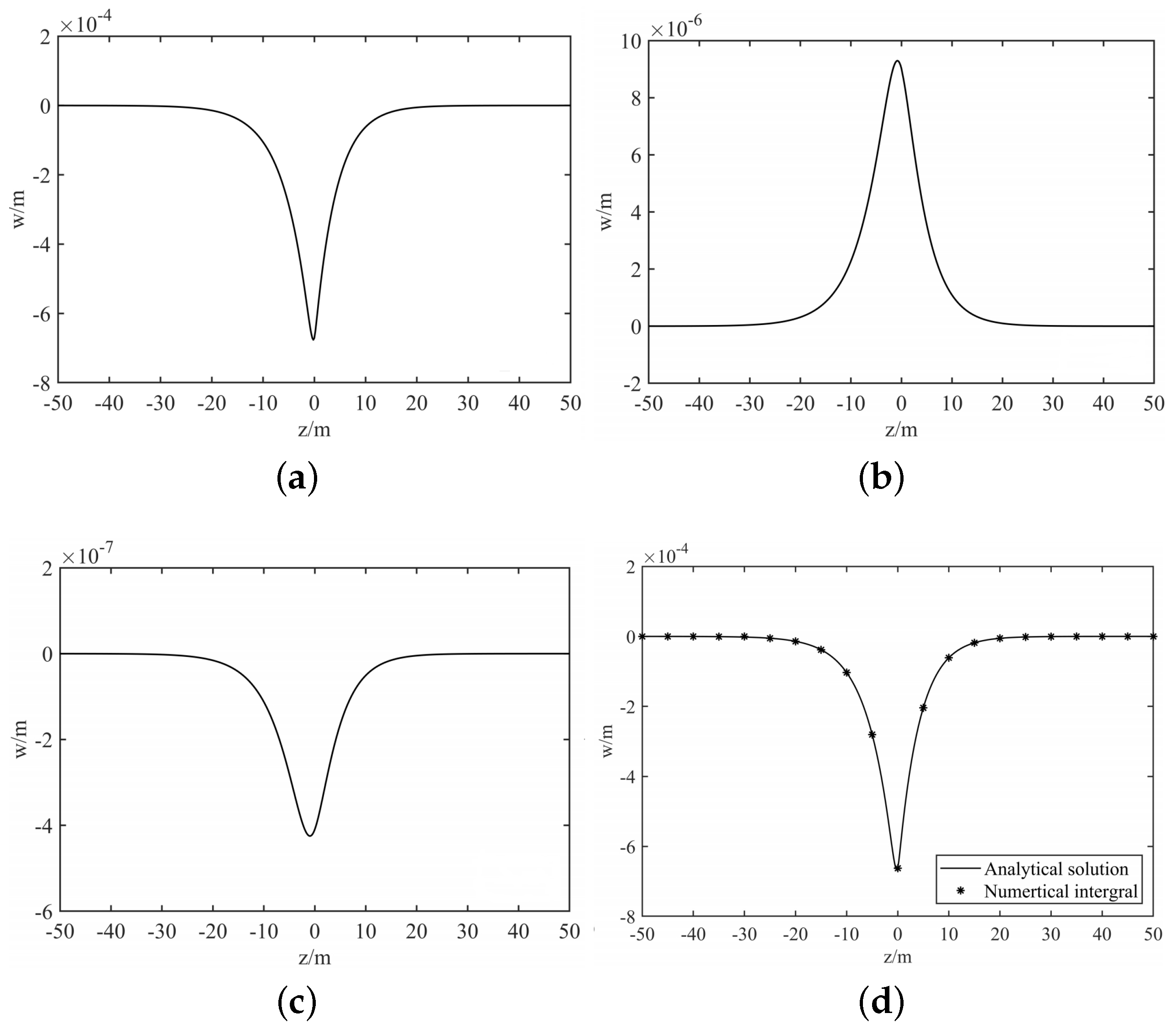
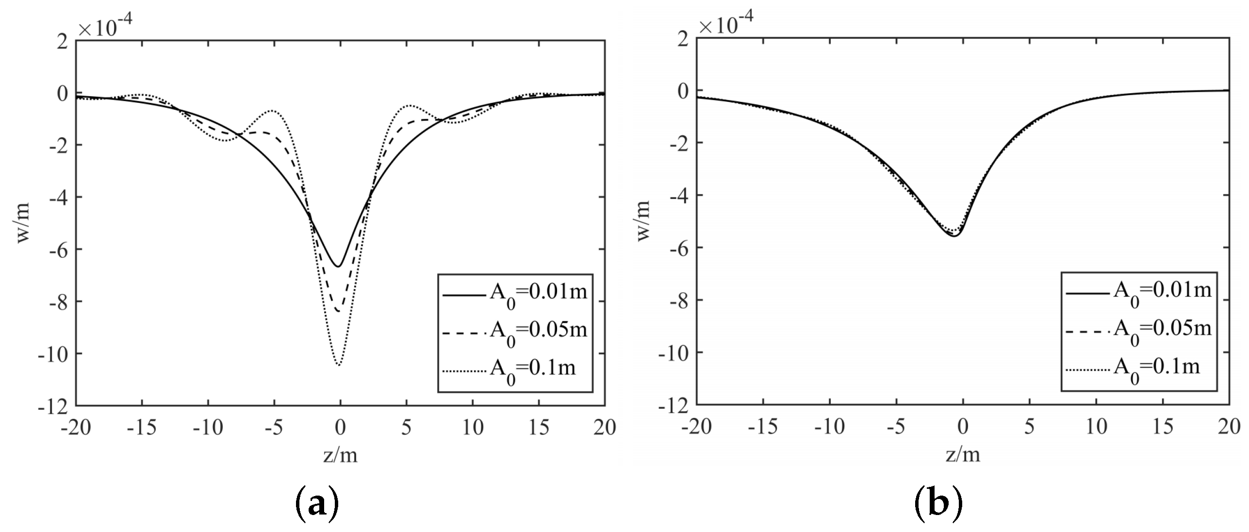
In this section, we initially validate the accuracy of the previous section’s analytical results by comparing them with numerical integration outcomes. Subsequently, we examine how different parameters, especially nonlinear stiffness, influence the vertical displacement of the pavement. Taking into account that the pavement is infinitely long and the vehicle velocity is constant, placing the coordinate system on the vehicle and setting $t=0$ can demonstrate the maximum amplitude of the pavement. The vehicle’s position serves as the reference origin for our comparative analysis.

3.1. The E-B Model

The beam, foundation, and vehicle load parameters for the numerical simulation of the E-B beam model are shown in

Table 1. Properties of the E-B beam, foundation [11] and vehicle [45].

Variable	Item	Notation	Value
Beam	Young’s modulus	E	$6.998\times {10}^9$ Pa
	Mass per unit Length	m	711.9 kg/m
	Sectional moment of inertia	I	$2.25\times {10}^{-3}$ m4
Roughness	Wavelength	$L_0$	10 m
	Amplitude	$A_0$	0.01 m
Foundation	Linear stiffness	k	$8\times {10}^6$ N/m2
	Nonlinear stiffness	$k_N$	$8\times {10}^{11}$ N/m4
	Viscous damping	c	$3\times {10}^5$ N·s/m2
Vehicle	Wheel mass	$m_1$	550 kg
	Suspension mass	$m_2$	4450 kg
	Tire stiffness	$K_1$	$1.75\times {10}^6$ N/m
	Suspension stiffness	$K_2$	$1\times {10}^6$ N/m
	Tire damping	$C_1$	$2\times {10}^3$ N·s/m2
	Suspension damping	$C_2$	$1.5\times {10}^4$ N·s/m2
	velocity	v	30 m/s

.

Figure 2 presents the variation in tire contact force over time. It can be observed from the figure that when the pavement roughness is a sine function, the tire contact force is a harmonic load that varies with time.

Using the parameters from Table 1, we calculate the vertical displacement of the pavement through Equation (19). According to Equation (18), it can be derived that

$$\begin{array}{cc}\hfill & ∥w_0∥=1.83\times {10}^{-3},∥w_1∥=3.08\times {10}^{-4},∥w_2∥=1.56\times {10}^{-4},\hfill \\ \hfill & {\varphi }_0={\displaystyle \frac{∥w_1∥}{∥w_0∥}}={\displaystyle \frac{3.08\times {10}^{-4}}{1.83\times {10}^{-3}}}\approx 0.168<1,\hfill \\ \hfill & {\varphi }_1={\displaystyle \frac{∥w_2∥}{∥w_1∥}}={\displaystyle \frac{1.56\times {10}^{-4}}{3.08\times {10}^{-4}}}\approx 0.506<1.\hfill \end{array}$$

(26)

Thus, the analytical solution derived from Equation (19) quickly converges to the precise solution of Equation (10). Figure 3 illustrates a comparison of the analytical solution for Equation (10) with numerical integration outcomes. It demonstrates that for this problem, summing the initial three terms of $w_j$ provides a close approximation to the actual value. Next, we focus on analyzing the impact of parameters on the vertical displacement of the beam using Equation (19).

Figure 4 shows the impact of pavement roughness amplitude variation on pavement deformation at different vehicle velocities, with all other parameters taking the values from Table 1. It can be seen from the figure that at lower vehicle velocity, the pavement deformation increases as the amplitude $A_0$ increases. However, when $A_0$ continues to increase, the pavement deformation remains almost unchanged. At higher vehicle velocity, the pavement deformation decreases as $A_0$ increases. But when $A_0$ continues to grow, the pavement deformation is hardly affected.

Figure 5 demonstrates how varying vehicle velocities and the nonlinear stiffness of the foundation affect the pavement response, given that $A_0$ = 0.01 m and all other parameters are fixed as per the values in Table 1. From Figure 5, it can be observed that when the coefficient $k_N$ is relatively small, it has almost no effect on the vertical deformation of the pavement; as $k_N$ increases, the maximum displacement of the pavement decreases slightly; when $k_N$ is further increased, there is a significant and substantial increase in the maximum displacement of the pavement. Comparing the pavement displacement at different velocities in Figure 5, the value of the nonlinear stiffness that affects displacement increases with increasing velocity. In other words, at higher velocities, a greater nonlinear stiffness is required to affect the maximum displacement of the pavement.

Figure 6 depicts the influence of varying vehicle velocities and the nonlinear stiffness on the pavement deformation, under the condition that $A_0$ = 0.05 m and with all remaining parameters aligning with the specifications detailed in Table 1. Comparing Figure 5 and Figure 6, the influence of vehicle velocity and nonlinear stiffness on pavement deformation is consistent under different pavement excitation amplitudes. Additionally, the position where the tire is located is not where the pavement experiences the greatest deformation, and the larger the $k_N$ value, the more pronounced this effect becomes.

Figure 7 and Figure 8 display the impact of varying viscous damping coefficients and the nonlinear stiffness of the foundation on pavement deformation at different vehicle velocities, with all other parameters set to the values listed in Table 1. It can be observed from the two figures that under varying foundation damping coefficients and vehicle velocities, there still exists a critical value for the nonlinear stiffness coefficient. When $k_N$ is less than the critical value, the pavement deformation remains largely unaffected by increases in $k_N$. When $k_N$ exceeds the critical value, the pavement deformation initially decreases and subsequently experiences a significant increase as $k_N$ grows. The critical value is influenced by both the foundation damping coefficient and the vehicle velocity; the greater the velocity and damping coefficient, the larger the critical value.

From the analysis of parameter influences in this subsection, it can be concluded that the impact of the foundation’s nonlinear stiffness on pavement deformation during vehicle travel is quite complex. For the nonlinear stiffness coefficient $k_N$, there exists a critical value, denoted as $k_{N0}$. If $k_N<k_{N0}$, changes in $k_N$ have almost no effect on pavement deformation; if $k_N>k_{N0}$, the deformation of the pavement initially diminishes and later escalates with the escalation of $k_N$. The critical value $k_{N0}$ is not fixed and is mainly related to vehicle velocity, foundation damping coefficient. An increase in vehicle velocity and foundation damping coefficient will significantly increase the value of $k_{N0}$. Changes in the pavement excitation amplitude do not significantly affect the critical value $k_{N0}$.

3.2. The Timoshenko Model

Table 2 displays the parameters of the beam and foundation utilized for the numerical simulation of the Timoshenko beam model. The vehicle parameters are taken from the values listed in Table 1. Similar to the previous subsection, the correctness of the analytical results is first verified. By substituting the parameter values from Table 1 and Table 2 into Equation (25), one can calculate

$$\begin{array}{cc}\hfill & ∥w_0∥=6.763\times {10}^{-4},∥w_1∥=9.134\times {10}^{-6},∥w_2∥=4.249\times {10}^{-7},\hfill \\ \hfill & {\varphi }_0={\displaystyle \frac{∥w_1∥}{∥w_0∥}}={\displaystyle \frac{9.134\times {10}^{-6}}{6.763\times {10}^{-4}}}\approx 0.0135<1,\hfill \\ \hfill & {\varphi }_1={\displaystyle \frac{∥w_2∥}{∥w_1∥}}={\displaystyle \frac{4.249\times {10}^{-7}}{9.134\times {10}^{-6}}}\approx 0.0465<1.\hfill \end{array}$$

(27)

Therefore, the approximate analytical solution obtained from Equation (25) will rapidly converge to the actual solution of Equation (20). Figure 9 presents the first three terms of $w_j$, along with a comparison between the approximate analytical solution and the numerical solution, demonstrating that Equation (25) is sufficiently accurate for discussing the impact of parameters on pavement deformation.

Figure 10 demonstrates how changes in the amplitude of pavement roughness affect pavement deformation across a range of vehicle velocities, using parameters as specified in Table 1 and Table 2. At lower vehicle velocities, pavement deformation increases with the growth of $A_0$; at higher vehicle velocities, pavement deformation is virtually unaffected by changes in $A_0$. Comparing Figure 10 with Figure 4, the patterns of influence by $A_0$ in the two different models are broadly similar, with the difference being that an increase in $A_0$ imparts a more pronounced fluctuation to the pavement deformation simulated by the Timoshenko beam model.

Table 2. Properties of the Timoshenko beam and foundation [11].

Variable	Item	Notation	Value
Beam	Young’s modulus	E	$6.998\times {10}^9$ Pa
	Shear modulus	G	$7.7\times {10}^{10}$ Pa
	Mass density	$\rho$	2373 kg/m3
	Cross sectional area	A	0.3 m2
	Sectional moment of inertia	I	$2.25\times {10}^{-3}$ m4
	Shear coefficients	$\lambda$	0.4
Roughness	Wavelength	$L_0$	10 m
	Amplitude	$A_0$	0.01 m
Foundation	Linear stiffness	$k_1$	$8\times {10}^6$ N/m2
	Nonlinear stiffness	$k_3$	$8\times {10}^{11}$ N/m4
	Viscous damping	c	$3\times {10}^5$ N·s/m2
	Shear parameter	$G_p$	$6.669\times {10}^7$ N
	Rocking stiffness	$k_f$	$1\times {10}^8$ N/m2
	Rocking damping	$c_f$	$1.5\times {10}^6$ N·s/m2

Table 2. Properties of the Timoshenko beam and foundation [11].

Variable	Item	Notation	Value
Beam	Young’s modulus	E	$6.998\times {10}^9$ Pa
	Shear modulus	G	$7.7\times {10}^{10}$ Pa
	Mass density	$\rho$	2373 kg/m3
	Cross sectional area	A	0.3 m2
	Sectional moment of inertia	I	$2.25\times {10}^{-3}$ m4
	Shear coefficients	$\lambda$	0.4
Roughness	Wavelength	$L_0$	10 m
	Amplitude	$A_0$	0.01 m
Foundation	Linear stiffness	$k_1$	$8\times {10}^6$ N/m2
	Nonlinear stiffness	$k_3$	$8\times {10}^{11}$ N/m4
	Viscous damping	c	$3\times {10}^5$ N·s/m2
	Shear parameter	$G_p$	$6.669\times {10}^7$ N
	Rocking stiffness	$k_f$	$1\times {10}^8$ N/m2
	Rocking damping	$c_f$	$1.5\times {10}^6$ N·s/m2

Figure 11 and Figure 12 show the influence of different vehicle velocities and the nonlinear stiffness of the foundation on the pavement response, with $A_0$ set to $0.01m$ and $0.05m$, respectively, and all other parameters maintained at the values listed in Table 1 and Table 2. The two figures reveal that for the nonlinear stiffness coefficient $k_3$, a threshold exists. If $k_3$ is less than the threshold, pavement deformation stays constant with an increase in $k_3$. Beyond this threshold, the pavement deformation first experiences a minor reduction and then escalates notably as $k_3$ rises. The critical value for $k_3$ is not static; it increases in conjunction with the vehicle velocity’s acceleration. Upon examining Figure 11 and Figure 12 in contrast to Figure 5 and Figure 6, it becomes clear that the wheel’s location does not coincide with the area of the pavement that undergoes the most significant deformation. Instead, there is a noticeable deviation between the two. When simulating the pavement with an E-B beam, this offset is quite pronounced and increases with the rise in nonlinear stiffness. However, when using a Timoshenko beam for the simulation, such offset is negligible and almost ignorable.

Figure 13 and Figure 14 illustrate the effects of different viscous damping coefficients and nonlinear stiffness coefficients of the foundation on the deformation of the pavement at various vehicle velocities, using all other parameters as specified in Table 1 and Table 2. The two figures reveal that, across a range of foundation damping coefficients and vehicle velocities, a critical value for the nonlinear stiffness coefficient persists. From these figures, it is evident that below a certain critical threshold, an increase in $k_3$ has minimal impact on pavement deformation. However, once $k_3$ surpasses this critical value, initially, the pavement deformation experiences a slight reduction, followed by a marked increase as $k_3$ continues to rise. The extent of this critical threshold is affected by the foundation’s damping coefficient and the vehicle’s velocity, with higher values of velocity and damping leading to a higher critical threshold.

The subsection’s parameter analysis reveals that the effect of the foundation’s nonlinear stiffness on pavement deformation during vehicle movement is intricate. For the nonlinear stiffness coefficient $k_3$, a critical threshold, referred to as $k_{30}$, is identified. Should $k_3$ be less than $k_{30}$, it minimally affects pavement deformation; nevertheless, if $k_3$ exceeds $k_{30}$, the deformation will initially drop and then ascend in tandem with the increase in $k_3$. The value of $k_{30}$ is not static, it fluctuates with variables such as vehicle velocity, the foundation’s damping coefficient, and the amplitude of pavement excitation. Specifically, an uptick in velocity and damping within the foundation notably raises $k_{30}$. Conversely, alterations in the amplitude of pavement excitation have a negligible effect on the critical threshold $k_{30}$. Comparing the analysis from the previous subsection, a critical value of foundation nonlinear stiffness, $k_{N0}$, also exists in the E-B beam model; with all other parameters being equal, $k_{30}$ is significantly larger than $k_{N0}$.

4. Discussion

In this section, we further compare the dynamic response of the E-B beam and the Timoshenko beam, as well as the critical values of nonlinear stiffness. Figure 15 illustrates the dynamic responses of E-B and Timoshenko beams when the vehicle speed, viscous damping coefficient, and foundation nonlinear stiffness coefficient are all the same, with $A_0=0.05\mathrm{m}$, and other parameters taken from Table 1 and Table 2. From Figure 15, it can be observed that when all parameters are the same, the maximum deformation of the E-B beam is significantly higher than that of the Timoshenko beam. As the viscous damping coefficient increases, the gap between the deformations of the two types of beams begins to narrow. Moreover, the critical value of nonlinear stiffness corresponding to the E-B beam is much smaller than that of the Timoshenko beam. When the nonlinear stiffness exceeds the critical value, the position of the maximum displacement on the beam starts to noticeably deviate from the wheel position. When the nonlinear stiffness of both types of beams is either less than or greater than their respective critical values, the offset between the maximum displacement and the wheel position is almost the same for both beams, aside from the difference in maximum deformation. The greatest difference between the two beams occurs when the nonlinear stiffness is just between the critical thresholds of the two types of beams.

This indicates that in pavement design, if the nonlinear stiffness is very small or very large, the dynamic behavior of the two types of beams will be relatively close, with the only difference being that the results calculated using the E-B beam are larger than those using the Timoshenko beam. In this case, the results obtained using the E-B beam are always on the safe side. However, if the nonlinear stiffness of the foundation is just between the critical values of the two types of beams, the difference in their dynamic behavior is the greatest. At this point, using the E-B beam does not guarantee the reliability of the calculated results.

5. Conclusions

In this research, we analytically investigate the dynamic response of the pavement subjected to a moving load from a vehicle, modeled as a two-degree-of-freedom system. The pavement is simulated with both the E-B beam and the Timoshenko beam theories, while the foundation is approximated by a nonlinear viscoelastic Winkler foundation featuring cubic characteristics. Using the Adomian decomposition method, combined with the Fourier transform and Duhamel’s integral, an integral form of the analytical solution for pavement deformation under the action of vehicles is obtained. Based on the analytical results, we conducted an in-depth study on the influence of the foundation’s nonlinear stiffness on the pavement deformation. The conclusions are as follows:

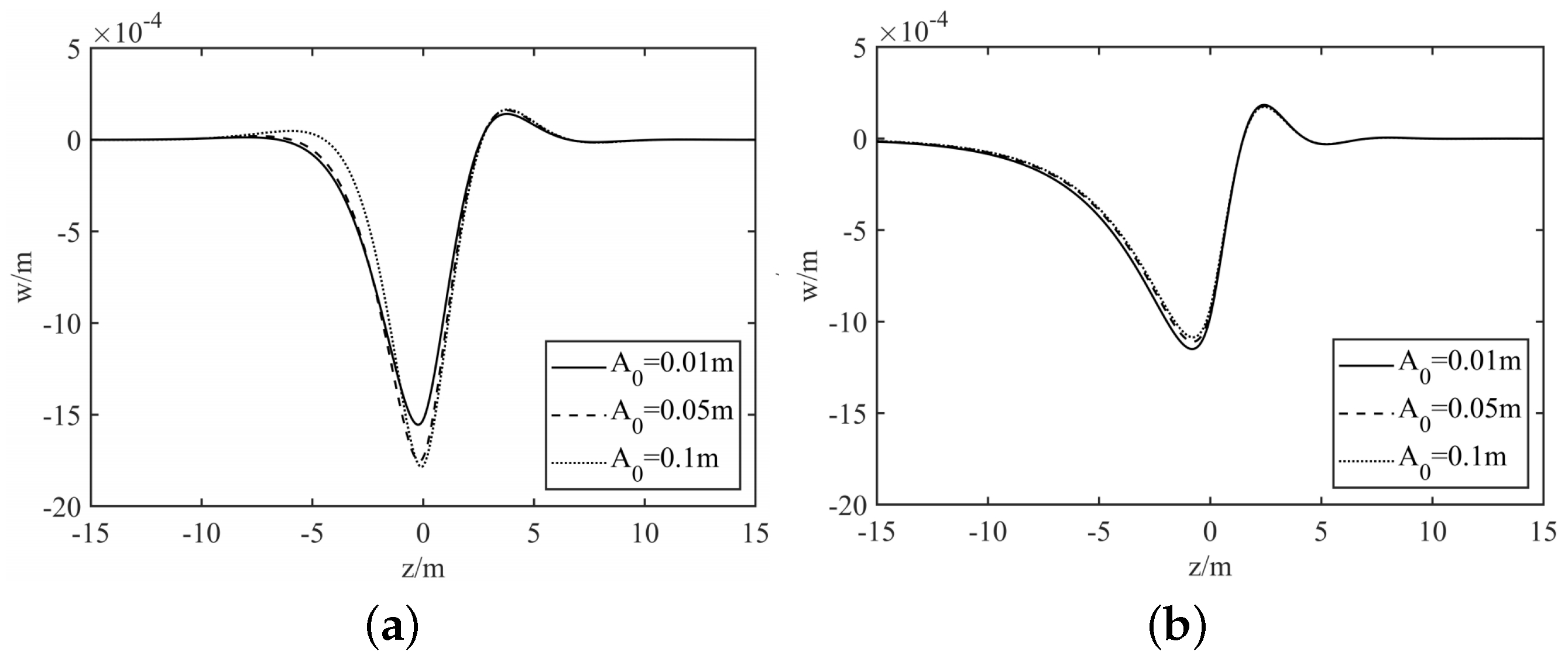
• When the excitation of the pavement takes the form of a sine wave, the force exerted by the tire upon contact is a harmonic load.
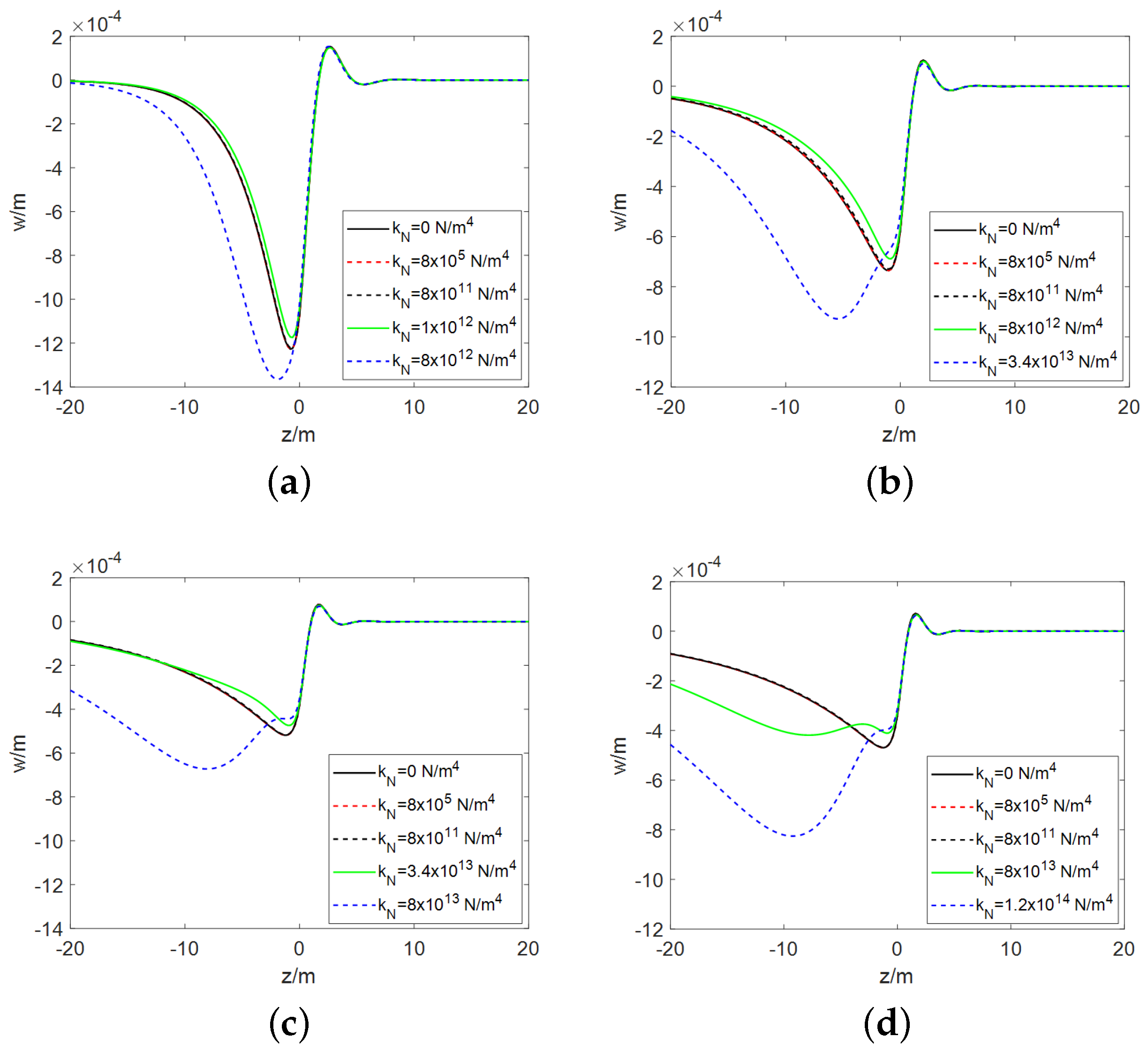
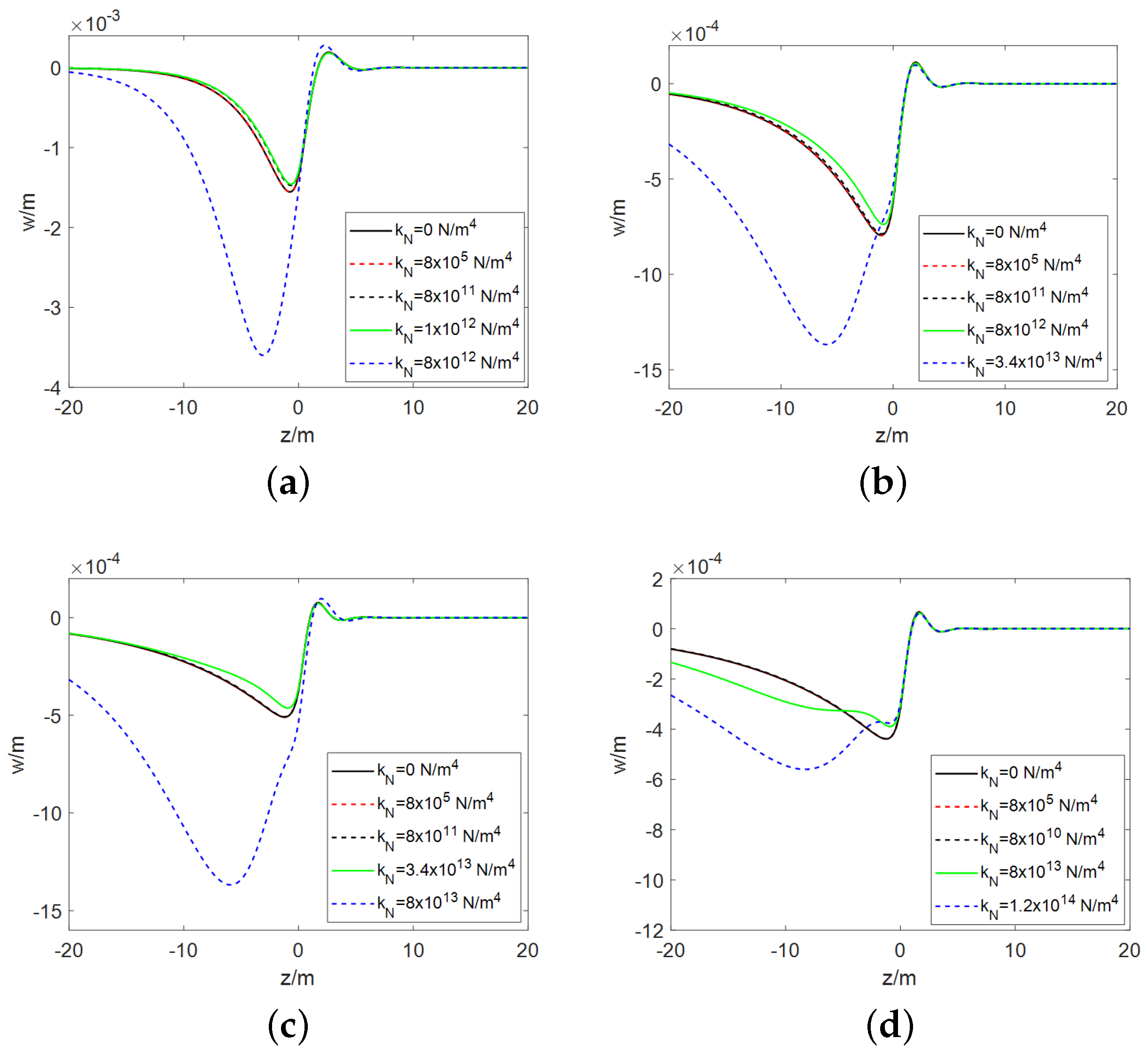
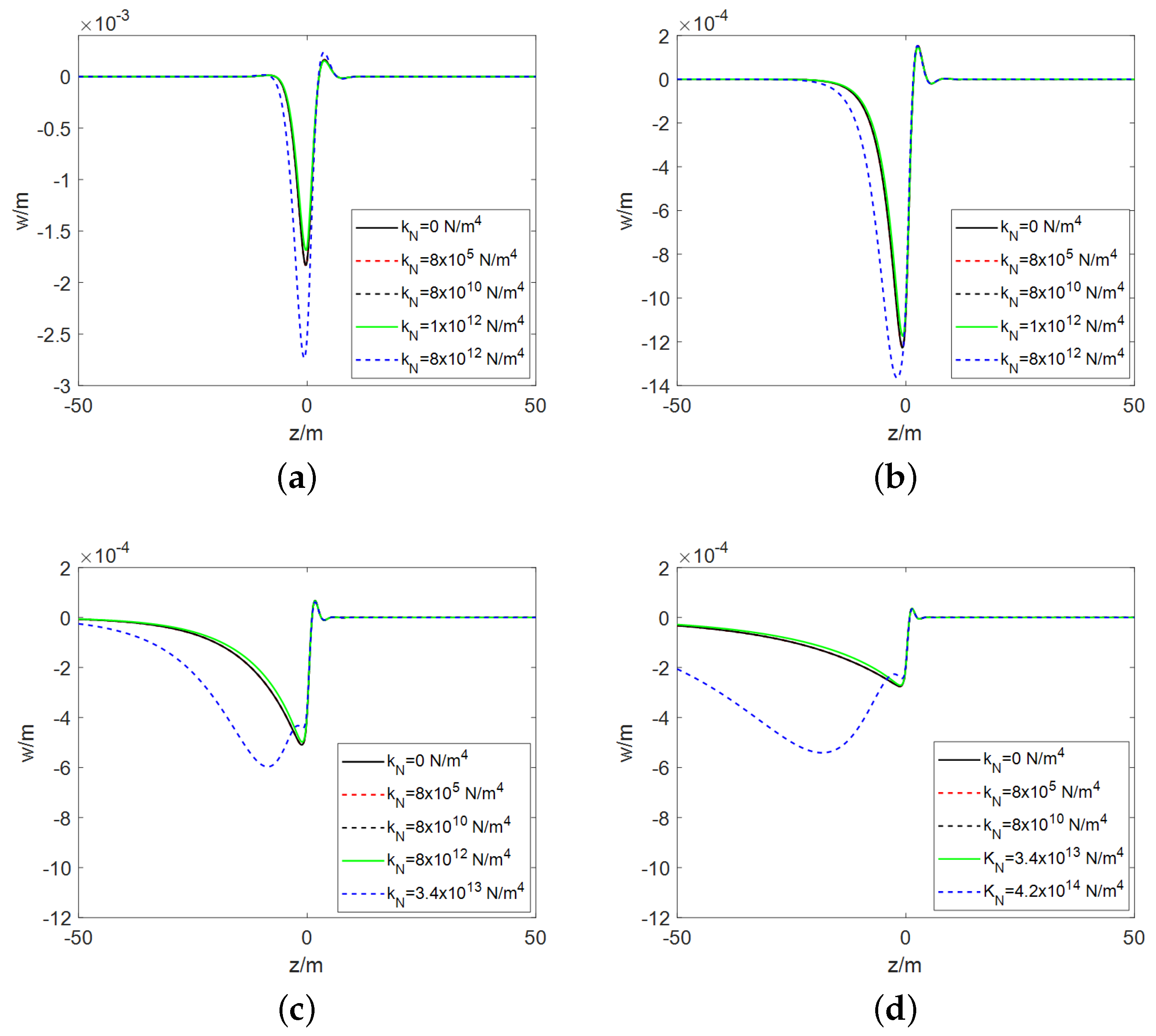
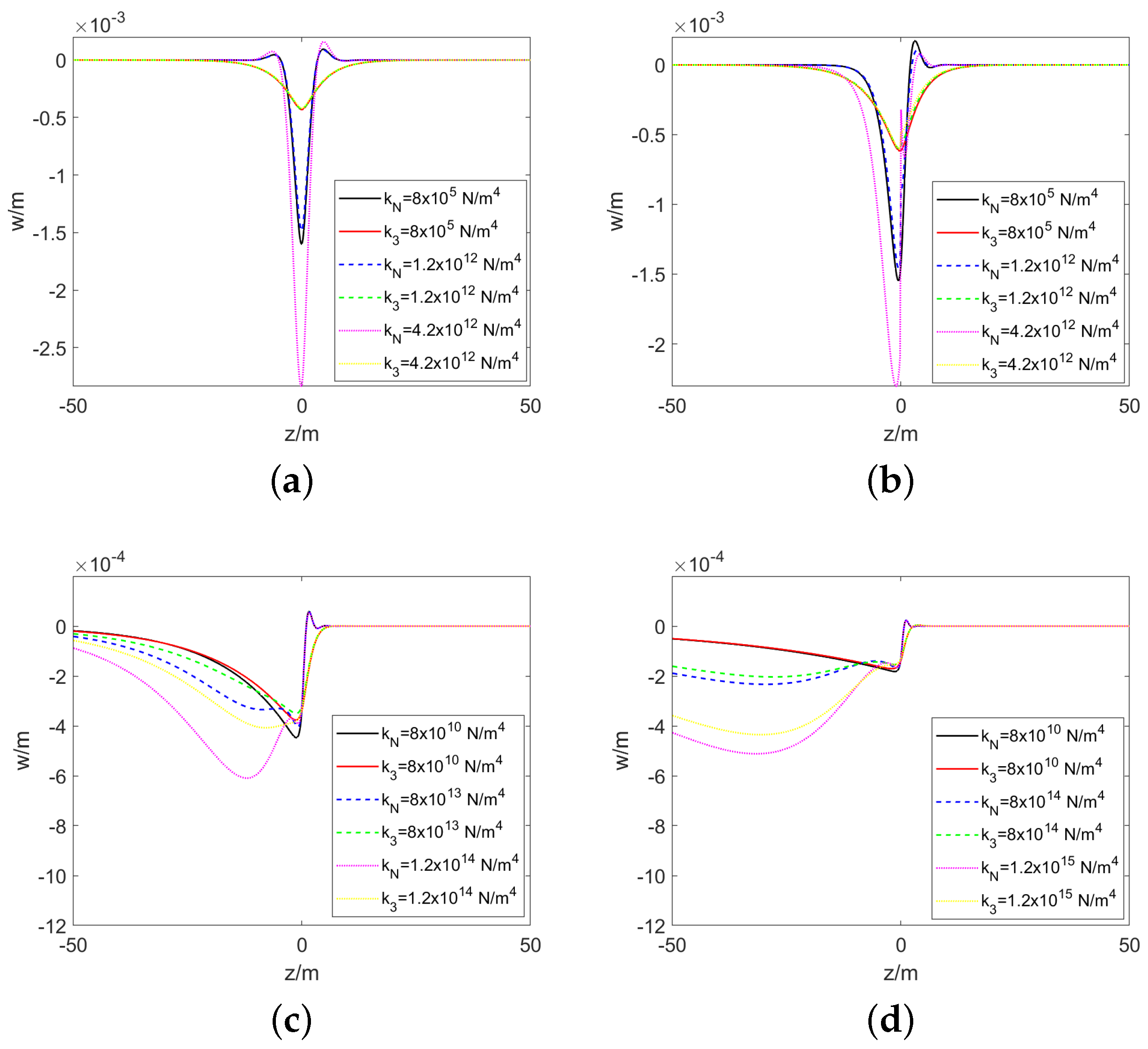
• Regardless of whether it is the E-B beam model or the Timoshenko beam model, the presence of cubic nonlinear stiffness will lead to an increase in the higher harmonic terms in the pavement response.
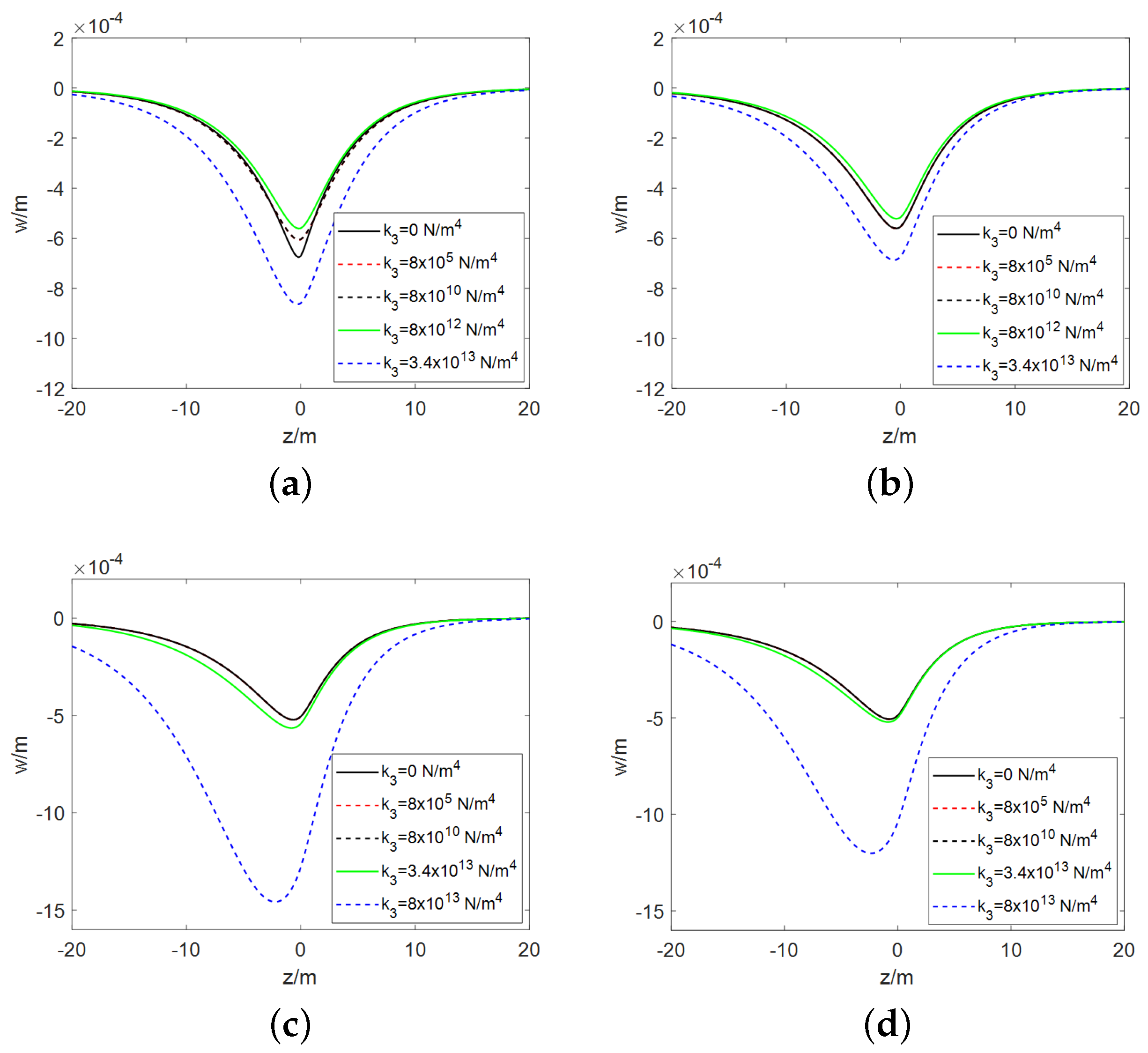
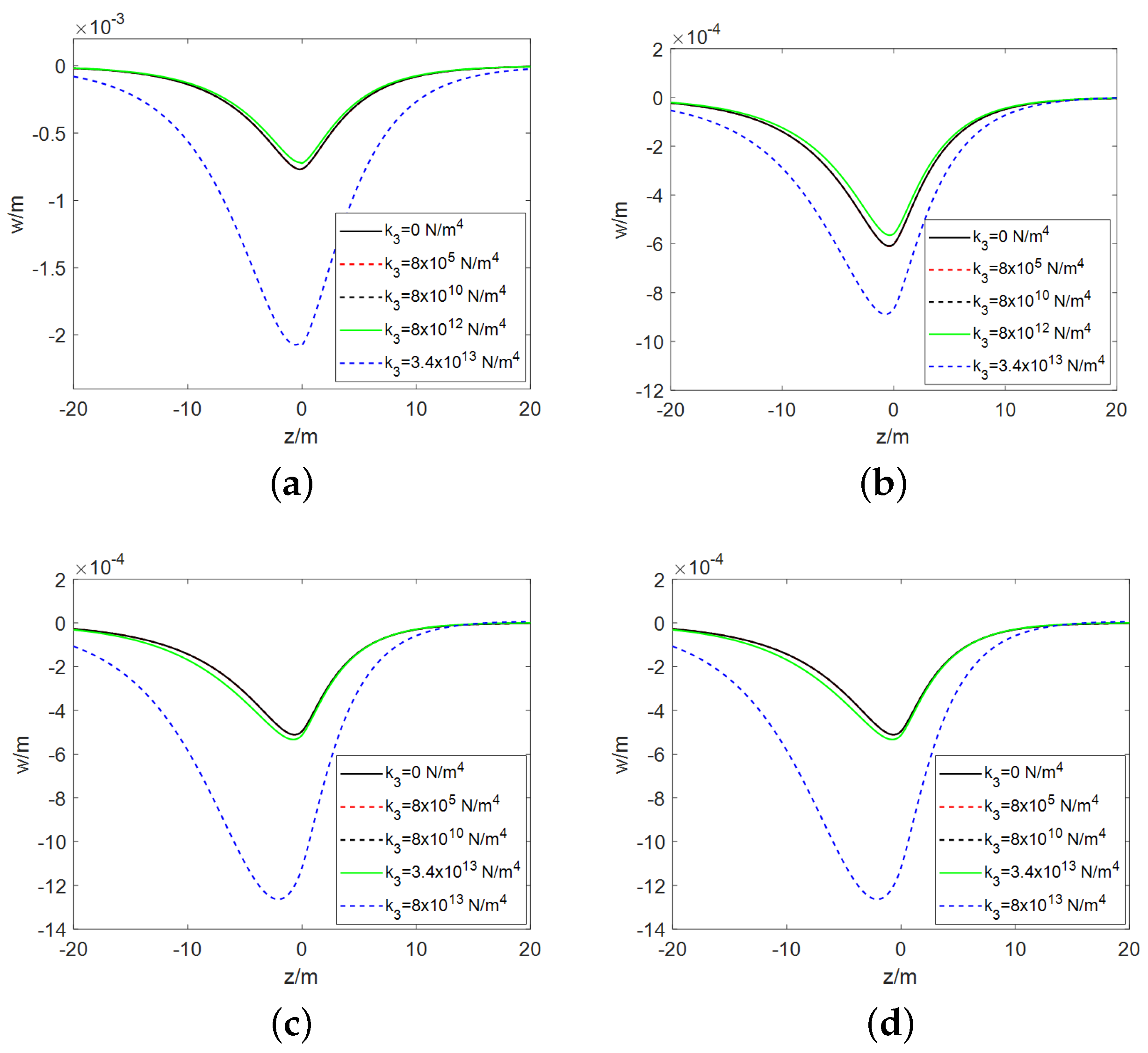
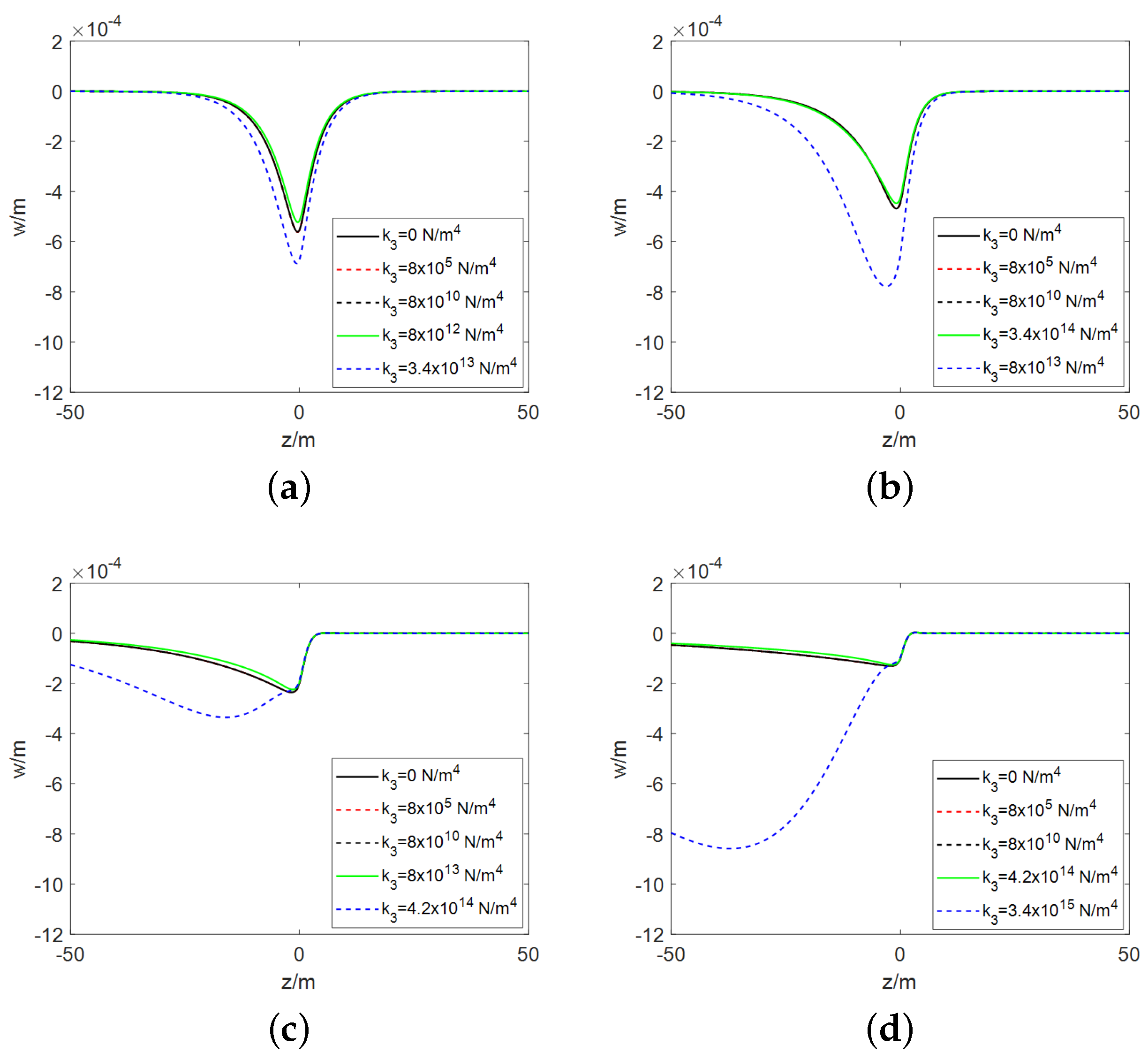
• Both the E-B beam model and the Timoshenko beam model have a threshold for the nonlinear stiffness of the foundation. When the nonlinear stiffness is below this threshold, its impact on the pavement deformation is negligible or minimal. However, when the nonlinear stiffness exceeds the threshold, the pavement deformation initially experiences a minor reduction, which is then followed by a substantial increase as the nonlinear stiffness rises. The magnitude of this threshold is not fixed and is primarily influenced by the vehicle velocity and the foundation damping coefficient, increasing with higher vehicle velocities and greater foundation damping. Under the same parameters, the threshold for the Timoshenko beam is significantly higher than that for the E-B beam.
• For both beam models, when the nonlinear stiffness is relatively low, the position of the wheel is almost coincident with the location of maximum pavement deformation. As the nonlinear stiffness increases, a noticeable offset occurs between the two positions, with the wheel positioned ahead of the area where the pavement deforms the most. The greater the nonlinear stiffness, the larger the offset between them. Comparatively, the offset effect is more pronounced in the E-B beam model.

In previous studies [46,47,48,49,50,51], it was commonly presumed that the beam was subjected to a moving force of unvarying magnitude. When the magnitude of the force is small, the foundation’s nonlinear stiffness has minimal impact on the beam deformation. However, when the force is substantial, the deformation of the beam increases with the growing nonlinear stiffness [8]. Under identical parameter conditions, the results derived from the E-B beam model are consistently higher than those from the Timoshenko beam model. Consequently, employing an E-B beam in design calculations for dynamic strength and fatigue is acceptable as it leads to an overestimation [52,53]. In this paper, the force acting on the beam is harmonic, and the research indicates that, under the same parameter conditions, the maximum deformation calculated using the E-B beam model exceeds that of the Timoshenko beam model. When the nonlinear stiffness is not significant, it is feasible to disregard the nonlinearity and use a linear model. When the nonlinear stiffness is considerable, there is a marked difference in the deformation distribution calculated by the E-B beam model compared to that of the Timoshenko beam model. If the concern extends beyond just the maximum value of deformation and also includes the discussion of deformation distribution along the beam, careful consideration in model selection is necessary. Our research results notably deepen the comprehension of the sophisticated, nonlinear mechanics that govern the dynamics of interactions between vehicles and pavements.

References

1. Niki, D.B.; Edmond, V.M. Review on dynamic response of road pavements to moving vehicle loads; part 1: Rigid pavements. Soil Dyn. Earthq. Eng. 2023, 175, 108249. [Google Scholar]
2. Niki, D.B.; Edmond, V.M. Review on dynamic response of road pavements to moving vehicle loads; part 2: Flexible pavements. Soil Dyn. Earthq. Eng. 2023, 175, 108248. [Google Scholar]
3. Wang, Y.; Li, S.W.; Wei, N. Dynamic response impact of vehicle braking on simply supported beam bridges with corrugated steel wE-Bs based on vehicle-bridge coupled vibration analysis. Comput. Model. Eng. Sci. 2024, 139, 3467–3493. [Google Scholar]
4. Ma, L.; Li, Z.; Xu, H.; Cai, C.S. Numerical study on the dynamic amplification factors of highway continuous beam bridges under the action of vehicle fleets. Eng. Struct. 2024, 304, 117638. [Google Scholar] [CrossRef]
5. Zhai, W.; Cai, Z. Dynamic interaction between a lumped mass vehicle and a discretely supported continuous rail track. Comput. Struct. 1997, 63, 987–997. [Google Scholar] [CrossRef]
6. Yuan, Z.H.; Xu, D.T.; Shi, L.; Pan, X.D.; He, B.; Hu, M.Y.; Cai, Y.Q. Hybrid analytical numerical modelling of ground vibrations from moving loads in a tunnel embedded in the saturated soil. Eur. J. Environ. Civil Eng. 2021, 26, 6047–6075. [Google Scholar] [CrossRef]
7. AASHTO. Mechanistic-Empirical Pavement Design Guide: A Manual of Practice; American Association of State Highway and Transportation Officials: Washington, DC, USA, 2020. [Google Scholar]
8. Ding, H.; Shi, K.L.; Chen, L.Q.; Yang, S.P. Dynamic response of an infinite Timoshenko beam on a nonlinear viscoelastic foundation to a moving load. Nonlinear Dyn. 2013, 73, 285–298. [Google Scholar] [CrossRef]
9. Chi, Z.Z.; He, Y.P.; Naterer, G.F. Design optimization of vehicle suspensions with a quarter-vehicle model. Trans. Can. Soc. Mech. Eng. 2008, 32, 297–312. [Google Scholar] [CrossRef]
10. Zhang, R.; Wang, X. Parameter study and optimization of a half-vehicle suspension system model integrated with an arm-teeth regenerative shock absorber using taguchi method. Mech. Syst. Signal Process. 2019, 126, 65–81. [Google Scholar] [CrossRef]
11. Yang, Y.; Ding, H.; Chen, L.Q. Dynamic response to a moving load of a timoshenko beam resting on a nonlinear viscoelastic foundation. Acta Mech. Sin. 2013, 29, 718–727. [Google Scholar] [CrossRef]
12. Sun, L.; Cai, X.M.; Yang, J. Genetic algorithm-based optimum vehicle suspension design using minimum dynamic pavement load as a design criterion. J. Sound Vib. 2007, 301, 18–27. [Google Scholar] [CrossRef]
13. Sarker, D.; Wang, J.X.; Khan, M.A. Development of the Virtual Load Method by Applying the Inverse Theory for the Analysis of Geosynthetic-Reinforced Pavement on Expansive Soils. In Proceedings of the Eighth International Conference on Case Histories in Geotechnical Engineering (GEO-CONGRESS 2019), Philadelphia, PA, USA, 24–27 March 2019. [Google Scholar]
14. Khan, M.A.; Wang, J.X. Application of Euler–Bernoulli Beam on Winkler Foundation for Highway Pavement on Expansive Soils. In Proceedings of the 2nd Pan-American Conference on Unsaturated Soils (PanAm-UNSAT), Dallas, TX, USA, 12–15 November 2017. [Google Scholar]
15. Zhang, M.; Jiang, X.; Liu, H.P.; Fu, Y.Q.; Abdelhaliem, B.L.E.; Qiu, Y.J. Development Optimization of Computer Programs for Asphalt Pavement Structure Based on Burmister’s Layered Theory from Application Perspective. Int. J. Pavement Res. Technol. 2024. [Google Scholar] [CrossRef]
16. Mamlouk, M.S. General outlook of pavement and vehicle dynamics. J. Transp. Eng. 1997, 123, 515–517. [Google Scholar] [CrossRef]
17. Fan, W.; Zhang, S.; Zhu, W.; Zhu, H. An efficient dynamic formulation for the vibration analysis of a multi-span power transmission line excited by a moving deicing robot. Appl. Math Model. 2022, 103, 619–635. [Google Scholar] [CrossRef]
18. Li, S.H.; Yang, S.P.; Chen, L.Q.; Lu, Y.J. Effects of parameters on dynamic responses for a heavy vehicle–pavement–foundation coupled system. Int. J. Heavy Veh. Syst. 2012, 19, 207–224. [Google Scholar] [CrossRef]
19. Li, S.H.; Yang, S.P.; Chen, L.Q. A nonlinear vehicle-road coupled model for dynamics research. J. Comput. Nonlinear Dyn. 2013, 8, 021001. [Google Scholar] [CrossRef]
20. Ding, H.; Yang, Y.; Chen, L.Q.; Yang, S.P. Vibration of vehicle–pavement coupled system based on a timoshenko beam on a nonlinear foundation. J. Sound Vib. 2014, 333, 6623–6636. [Google Scholar] [CrossRef]
21. Krishnanunni, C.G.; Rao, B.N. Decoupled technique for dynamic response of vehicle–pavement systems. Eng. Struct. 2019, 191, 264–279. [Google Scholar] [CrossRef]
22. Pirmoradian, M.; Torkan, E.; Karimpour, H. Parametric resonance analysis of rectangular plates subjected to moving inertial loads via IHB method. Int. J. Mech. Sci. 2018, 142, 191–215. [Google Scholar] [CrossRef]
23. Bucinskas, P.; Andersen, L.V. Dynamic response of vehicle-bridge-soil system using lumped-parameter models for structure-soil interaction. Comput. Struct. 2020, 238, 106270. [Google Scholar] [CrossRef]
24. Ma, X.Y.; Quan, W.W.; Dong, Z.J.; Dong, Y.K.; Si, C.D. Dynamic response analysis of vehicle and asphalt pavement coupled system with the excitation of road surface unevenness. Appl. Math. Model. 2022, 104, 421–438. [Google Scholar] [CrossRef]
25. Liou, J.Y.; Sung, J.C. Surface responses induced by point load or uniform traction moving steadily on an anisotropic half-plane. Int. J. Solid Struct. 2008, 45, 2737–2757. [Google Scholar] [CrossRef]
26. Dutykh, D. Moving Load on a Floating Ice Layer. Master’s Thesis, Khalifa University of Science and Technology, Abu Dhabi, United Arab Emirates, 2005. [Google Scholar]
27. Pegios, I.P.; Papargyri-Beskou, S.; Zhou, Y.; He, P. Steady-state dynamic response of a gradient elastic half-plane to a load moving on its surface with constant speed. Arch. Appl. Mech. 2019, 88, 1809–1824. [Google Scholar] [CrossRef]
28. Rys, D.; Burnos, P. Study on the accuracy of axle load spectra used for pavement design. Int. J. Pavement Eng. 2021, 23, 3706–3715. [Google Scholar] [CrossRef]
29. Zhu, X.Q.; Law, S.S. Structural health monitoring based on vehicle-bridge interaction: Accomplishments and challenges. Adv. Struct. Eng. 2015, 18, 1999–2015. [Google Scholar] [CrossRef]
30. Martínez, C.J.; Mazzola, L.; Baeza, L.; Bruni, S. Numerical estimation of stresses in railway axles using a train–track interaction model. Int. J. Fatigue 2013, 47, 18–30. [Google Scholar] [CrossRef]
31. Frýba, L. Vibration of Solids and Structures under Moving Loads; Springer Science & Business Media: Dordrecht, The Netherlands, 2013. [Google Scholar]
32. Cifuentes, A.O. Dynamic response of a beam excited by a moving mass. Finite Elem. Anal. Des. 1989, 5, 237–246. [Google Scholar] [CrossRef]
33. Sun, L. An explicit representation of steady state response of a beam on an elastic foundation to moving harmonic line loads. Int. J. Numer. Anal. Methods Geomech. 2003, 27, 69–84. [Google Scholar] [CrossRef]
34. Zhang, Y. Steady state response of an infinite beam on a viscoelastic foundation with moving distributed mass and load. Sci. China Phys. Mech. Astron. 2020, 63, 284611. [Google Scholar] [CrossRef]
35. Dimitrovová, Z. Complete semi-analytical solution for a uniformly moving mass on a beam on a two-parameter visco-elastic foundation with non-homogeneous initial conditions. Int. J. Mech. Sci. 2018, 144, 283–311. [Google Scholar] [CrossRef]
36. Chen, H.Y.; Ding, H.; Li, S.H.; Chen, L.Q. Convergent term of the Galerkin truncation for dynamic response of sandwich beams on nonlinear foundations. J. Sound Vib. 2020, 483, 115514. [Google Scholar] [CrossRef]
37. Zhen, B.; Xu, J.; Sun, J.Q. Analytical solutions for steady state responses of an infinite Euler–Bernoulli beam on a nonlinear viscoelastic foundation subjected to a harmonic moving load. J. Sound Vib. 2020, 476, 115271. [Google Scholar] [CrossRef]
38. Adomian, G.; Rach, R. Equality of partial solutions in the decomposition method for linear or nonlinear partial differential equations. Comput. Math. Appl. 1990, 19, 9–12. [Google Scholar] [CrossRef]
39. Snehasagar, G.; Krishnanunni, C.G.; Rao, B.N. Dynamics of vehicle–pavement system based on a viscoelastic Euler–Bernoulli beam model. Int. J. Pavement Eng. 2020, 21, 1669–1682. [Google Scholar] [CrossRef]
40. Zhang, S.H.; Fan, W.; Yang, C.J. Semi-analytical solution to the steady-state periodic dynamic response of an infinite beam carrying a moving vehicle. Int. J. Mech. Sci. 2022, 226, 107409. [Google Scholar] [CrossRef]
41. Wu, T.X.; Thompson, D.J. The effects of track non-linearity on wheel/rail impact. Proc. Inst. Mech. Eng. Part F J. Rail Rapid Transit 2004, 218, 1–15. [Google Scholar] [CrossRef]
42. Ding, H.; Chen, L.Q.; Yang, S.P. Convergence of Galerkin truncation for dynamic response of finite beams on nonlinear foundations under a moving load. J. Sound Vib. 2012, 331, 2426–2442. [Google Scholar] [CrossRef]
43. Yang, S.P.; Li, S.H.; Lu, Y.J. Investigation on dynamical interaction between a heavy vehicle and road pavement. Veh. Syst. Dyn. 2010, 48, 923–944. [Google Scholar] [CrossRef]
44. Wazwaz, A.M. Adomian decomposition method for a reliable treatment of Emden-Fowler equation. Appl. Math. Comput. 2003, 161, 543–560. [Google Scholar] [CrossRef]
45. Ma, X.Y.; Quan, W.W.; Dong, Z.J.; Si, C.D.; Li, S.H. Research on dynamic response of vehicle and asphalt pavement interaction under random unevenness Excitation. J. Mech. Eng. 2021, 57, 40–50. (In Chinese) [Google Scholar]
46. Ai, Z.Y.; Ren, G.P. Dynamic response of an infinite beam on a transversely isotropic multilayered half-space due to a moving load. Int. J. Mech. Sci. 2017, 133, 817–828. [Google Scholar] [CrossRef]
47. Fǎrǎgǎu, A.B.; Mazilu, T.; Metrikine, A.V.; Lu, T.; Van Dalen, K.N. Transition radiation in an infinite one-dimensional structure interacting with a moving oscillator-the Green’s function method. J. Sound Vib. 2021, 492, 115804. [Google Scholar] [CrossRef]
48. Liu, Z.H.; Niu, J.C.; Jia, R.H. Dynamic analysis of arbitrarily restrained stiffened plate under moving loads. Int. J. Mech. Sci. 2021, 200, 106414. [Google Scholar] [CrossRef]
49. Zhang, Y.; Liu, X. Response of an infinite beam resting on the tensionless Winkler foundation subjected to an axial and a transverse concentrated loads. Eur. J. Mech. A Solids 2019, 77, 103819. [Google Scholar] [CrossRef]
50. Phadke, H.; Jaiswal, O. Dynamic analysis of railway track on variable foundation under harmonic moving load. Proc. Inst. Mech. Eng. F J. Rail Rapid Transit 2022, 236, 302–316. [Google Scholar] [CrossRef]
51. Zhang, J.N.; Yang, S.P.; Li, S.H.; Ding, H.; Lu, Y.J.; Si, C.D. Study on crack propagation path of asphalt pavement under vehicle-road coupled vibration. Appl. Math. Model. 2022, 101, 481–502. [Google Scholar] [CrossRef]
52. Qiao, G.D.; Rahmatalla, S. Dynamics of Euler–Bernoulli beams with unknown viscoelastic boundary conditions under a moving load. J. Sound Vib. 2021, 491, 115771. [Google Scholar] [CrossRef]
53. Dimitrovová, Z. Dynamic interaction and instability of two moving proximate masses on a beam on a Pasternak viscoelastic foundation. Appl. Math. Model. 2021, 100, 192–217. [Google Scholar] [CrossRef]
Figure 1. The vehicle–pavement–foundation system.
Applsci 14 08705 g001
Figure 2. The tire contact force exerted by the vehicle on the pavement.
Applsci 14 08705 g002
Figure 3. Comparison between the approximate analytical solutions of Equation (10) and numerical results when the vehicle velocity is v = 30 m/s. (a) The first three terms of w j . (b) Comparison of two solutions.
Applsci 14 08705 g003
Figure 4. The impact of different vehicle velocities and pavement roughness amplitudes on the pavement response. (a) v = 30 m/s. (b) v = 90 m/s.
Applsci 14 08705 g004
Figure 5. The impact of different vehicle velocities and the nonlinear stiffness of the foundation on the pavement response when the pavement roughness amplitude is A 0 = 0.01 m. (a) v = 30 m/s. (b) v = 60 m/s. (c) v = 90 m/s. (d) v = 100 m/s.
Applsci 14 08705 g005
Figure 6. The impact of different vehicle velocities and the nonlinear stiffness of the foundation on the pavement response when the pavement roughness amplitude is A 0 = 0.05 m. (a) v = 30 m/s. (b) v = 60 m/s. (c) v = 90 m/s. (d) v = 100 m/s.
Applsci 14 08705 g006
Figure 7. The impact of different viscous damping coefficients and the nonlinear stiffness on the pavement response when the vehicle velocity is v = 30 m/s. (a) c = 3 × 10 5 N· s/m2. (b) c = 9 × 10 5 N· s/m2. (c) c = 3 × 10 6 N· s/m2. (d) c = 6 × 10 6 N· s/m2.
Applsci 14 08705 g007
Figure 8. The impact of different viscous damping coefficients and the coefficients of nonlinear stiffness on the pavement response when the vehicle velocity is v = 60 m/s. (a) c = 3 × 10 5 N· s/m2. (b) c = 9 × 10 5 N· s/m2. (c) c = 3 × 10 6 N· s/m2. (d) c = 6 × 10 6 N· s/m2.
Applsci 14 08705 g008
Figure 9. The first three terms of w j and the comparison between analytical solution in Equation (25) and numerical result for Equation (20). (a) w 0 . (b) w 1 . (c) w 2 . (d) Comparision of two solutions.
Applsci 14 08705 g009
Figure 10. The effects of varying vehicle velocities and amplitudes of pavement roughness on the pavement’s reactive performance. (a) v = 30 m/s. (b) v = 90 m/s.
Applsci 14 08705 g010
Figure 11. The impact of different vehicle velocities and the nonlinear stiffness coefficient of the foundation on the pavement response when the pavement roughness amplitude is A 0 = 0.01 m. (a) v = 30 m/s. (b) v = 60 m/s. (c) v = 90 m/s. (d) v = 100 m/s.
Applsci 14 08705 g011
Figure 12. The impact of different vehicle velocities and the nonlinear stiffness coefficient of the foundation on the pavement response when the pavement roughness amplitude is A 0 = 0.05 m. (a) v = 30 m/s. (b) v = 60 m/s. (c) v = 90 m/s. (d) v = 100 m/s.
Applsci 14 08705 g012
Figure 13. The effects of varying viscous damping coefficients and nonlinear stiffness coefficients on the pavement response are examined at a vehicle velocity of v = 30 m/s. (a) c = 3 × 10 5 N· s/m2. (b) c = 9 × 10 5 N· s/m2. (c) c = 3 × 10 6 N· s/m2. (d) c = 6 × 10 6 N· s/m2.
Applsci 14 08705 g013
Figure 14. The influence of assorted viscous damping factors and nonlinear stiffness factors of the foundation on the pavement’s reaction is depicted at a vehicle velocity of v = 60 m/s. (a) c = 3 × 10 5 N· s/m2. (b) c = 9 × 10 5 N· s/m2. (c) c = 3 × 10 6 N· s/m2. (d) c = 6 × 10 6 N· s/m2.
Applsci 14 08705 g014
Figure 15. Comparison of calculation results for the two types of beams under the same parameter conditions. (a) c = 3 × 10 5 N·s/m2, v = 10 m/s. (b) c = 9 × 10 5 N·s/m2, v = 20 m/s. (c) c = 3 × 10 6 N·s/m2, v = 40 m/s. (d) c = 6 × 10 6 N·s/m2, v = 50 m/s.
Applsci 14 08705 g015