Design of a Steady-State Adjustment Method and Sensitivity Analysis for an ORC System with Plate Heat Exchangers

Abstract

Because of its low concentration and low energy in an organic Rankine cycle (ORC) system, more than 50% of low-grade thermal energy with a temperature below 300 °C is not taken seriously. The relationship between changeable working condition parameters and operating parameters is typically not taken into account in a model while studying ORC systems. It is insufficient to analyze the system performance changes solely on changes in the performance parameters of the heat exchangers. Furthermore, a model perspective of the system control solution is absent from the steady-state control of the system when the heat source varies. In this paper, we created a system model for the application scenario of a 100–200 kW ORC system with brazed plate heat exchangers in order to address the aforementioned issues using MATLAB R2016b. Additionally, a sensitivity analysis of the system was conducted based on heat exchangers of performance variations. In addition, a modeling computation and adjustment scheme were put forth to guarantee that the system could continue to produce steady power production even when the temperature of the heat source fluctuated. Preliminary results showed that the system’s internal parameters included its evaporation pressure and condensation temperature. An increase in evaporation pressure will reduce the mass flow rate and heat flux of an evaporator, thus reducing the heat transfer coefficient. The two-phase region of the evaporator accounted for the highest proportion, of 70.22%, and continued to increase to 75.83%, followed by the supercooling region, and gradually decreasing. The utilization rate of the evaporator decreased from 74.85% to 38.32%. The system output power increased first and then decreased, with a maximum value of 153.11 kW. The system efficiency increased from 5.74% to 11.04%. The increase in condensation temperature increased the proportion of the two-phase region and the superheating region, and the mass flow rate did not change much. The increase in heat flux increased the heat transfer coefficient from 1721.31 W/(m²·K) to 2374.77 W/(m²·K), and the utilization rate of the evaporator decreased from 70.56% to 51.91%. The aforementioned change rules were used in the building of the steady-state regulation model to balance out the changes in the generating power as the heat source temperature increased. The model output was cross-checked and validated against pertinent experimental test literature data. The results of this research can serve as a valid and useful guide for ORC system design and practical applications.

1. Introduction

Although 60% of all energy is consumed in the industrial sector, less than 50% of that energy is used for waste heat utilization [1]. Because of its modest concentration and low energy, more than 50% of low-grade thermal energy at temperatures below 300 °C is not considered seriously [2]. After cooling, it is typically released straight into the atmosphere, wasting energy resources and polluting the environment. The Stirling cycle, Kalina cycle, triangle flash cycle, organic Rankine cycle (ORC), and other cycles are currently included in waste heat recovery. Low-boiling organics are used by the ORC as the working fluid among them. The ORC offers clear benefits because of its lower heat source temperature and pressure, liquid-free expansion process, and loose equipment requirements [3,4]. Furthermore, the ORC has over 50 years of experience with commercial applications. In the sphere of power generation, the cost can be recouped in 2.5 years on average. The prospects for applications are really bright. Systems for large-scale ORC equipment typically need steady power. The configuration and choice of heat exchangers have a significant effect on the performance of an ORC system since they are the piece of equipment with the biggest exergy loss. Therefore, when the external working conditions change greatly, the design and control of a multi-heat exchanger ORC system solution is particularly important. Consequently, the design and control of an ORC system solution with appropriate heat exchangers are especially crucial when the exterior working conditions change significantly.

1.1. ORC System

Over the past ten years, ORC system research has primarily concentrated on four key areas: the working fluid, numerical simulation, thermodynamic calculation and optimization, and experimental research.

For instance, a few researchers [5,6,7,8,9,10,11,12] have modeled and experimented with a variety of ORC types, including two-stage series, basic-type, extraction steam recovery, and reheating, as well as multi-objective system optimization. The low temperature and low density of low-temperature heat sources result in a high usage cost. System integration and cost benefits are typically less possible with more sophisticated system types [13,14]. Through neural networks and dynamic models, the optimal parameters for system operation can be successfully predicted. Additionally, they acquire the critical variables, assessment metrics, and influence guidelines that impact an ORC system’s thermal performance. By using energy analysis, optimization strategies for the system’s main components were suggested.

The selection of ORC working fluids has been extensively studied. More than 117 organic compounds, including R152a, R245fa, benzene, R134a, R113, ammonia, R123, R245ca, isobutylene, cyclohexane, isopentane, toluene, etc., have been the subject of studies by a number of researchers [15,16,17,18,19]. According to the different temperature levels of the heat source, organic working fluids are divided into two categories: high-temperature [20,21,22] and medium- and low-temperature working fluids [23,24,25,26]. The former has a relatively lower output power and efficiency using a low-temperature heat resource, mainly because the physical parameters such as the heat capacity of high-temperature working fluids such as MDM (octamethyltrisiloxane), MD2M (decamethyltetrasiloxane), and MM (hexamethyldisiloxane) are greatly affected by temperature [22], and the critical parameters are higher than the corresponding values of medium- and low-temperature working fluids. Their chemical properties and thermodynamic characteristics [21] are unstable. In addition, the inevitable mixing of oil and mineral lubricants during their operation can accelerate the decomposition of the working fluid, resulting in a decrease in system performance [20]. In medium- and low-temperature-level systems of a heat source, the physical properties of the refrigerant are better than those of other organic substances. The system’s thermoeconomic parameters such as the output power, efficiency, and cost were mainly affected by the heat source temperature range, the critical temperature of the refrigerant, the boiling temperature, and the pinch point temperature difference. The research of Yang et al. [23] showed that when the heat source temperature was in the range of 423.15–473.15 K, the maximum output power of their ORC system was affected by the critical temperature of the working fluid, but had nothing to do with the boiling point value. Zhai et al. [24] compared and evaluated the system exergy efficiency of 30 working fluids with critical temperatures ranging from 71.87 °C to 357.65 °C. Different heat sources and working conditions lead to different optimal working fluids. The key parameter is the critical temperature, which is determined by the heat source temperature, the pinch temperature difference, and the condensation temperature. Ye et al. [25] analyzed the economic benefits of the R12333zd(E), R1234ze(Z), R1366mzz(E), and R245fa working fluids and conducted experimental verification. When the evaporation temperature was 127 °C and the condensation temperature was 30 °C, R12333zd(E) was the best, and R245fa was very close to it in terms of physical properties. Zekeriya et al. [26] evaluated 29 different single-component refrigerants. The study showed that the steam expansion ratio of the dry working fluid was directly related to the net output work. When R113 replaced R600, the thermal efficiency and exergy efficiency were increased by 0.59% and 3.18%, respectively, and the levelized electrical cost was reduced by about 11%.

Some other scholars [27,28,29,30] have performed detailed design and modeling calculations on the core components of the ORC system, which contains an evaporator, a condenser, a pump, and an expander. Analysis was also conducted on the primary thermal factors that impacted the functionality of core components and how those factors impacted other factors like the system efficiency. Those research results offer a useful point of reference for resolving the coupling issue between system and component models.

1.2. Variable Heat Source Temperature of an ORC System

Usually, the heat source driving an ORC is erratic and variable. Overheating of the system will result in an excessive rise in pressure and temperature, as well as a cracking of the working fluid. Liquid shock in the expander is caused by insufficient heat absorption in the system, which prevents normal system operation [31,32]. As a result, the system’s performance in relation to heat source modifications has received a lot of attention.

Manente et al. [33] focused on the characteristics of an ORC system driven by geothermal energy under off-design conditions and studied the optimal operating parameters and maximum power generation of the ORC system under seasonal heat source temperature and cold source temperature changes during year-round operation. The outcomes demonstrated that the ORC system’s output power would be significantly influenced by the cold source temperature. Francesco et al. [34] investigated a solar-driven ORC system’s changeable working condition performance, established a collector model using a lumped model, and obtained how the system’s pressure and thermal efficiency changed at various temperatures and thermal oil flow rates. A geothermal energy-driven integrated cooling, heating, power, and fresh water supply system was also simulated and its reaction to winter temperatures and energy flow under various operating situations was examined by Ref. [35]. Rongqi et al. [36] studied a flue gas waste heat recovery system. By adjusting the temperature and flow rate of the flue gas entering the evaporator, a stable evaporator pressure and temperature were obtained under the condition of fluctuations in the heat source temperature and flow rate. Xinle Yang et al. [37] proposed an ORC with a heat source-regulated (ORC-R) system. They deduced from modeling simulations that when the ORC-R system achieved its optimal performance value, its evaporation temperature would be lower than that of the basic ORC system. The performance of the system was optimized by a heat source adjustment coefficient.

1.3. Evaporators in an ORC

The heat exchanger is the component with the largest exergy loss and cost consumption in an ORC system. Common heat exchanger types include plate, shell-and-tube, and fin-tube heat exchangers. Bull et al. [38] compared the heat transfer efficiency of plate heat exchangers and shell-and-tube heat exchangers under varying evaporation pressures and concluded that the plate heat exchanger had a lower cold end area requirement of nearly 40% at each pressure level. Xu et al. [39] proposed a fuzzy normalized optimization screening method and used a genetic algorithm to realize the parametric optimization of the detailed models of a shell-and-tube heat exchanger and plate heat exchanger in an ORC. The heat transfer coefficient of the plate condenser was higher than that of the shell-and-tube heat exchanger, while the pressure drop was slightly higher. Similarly, Walraven et al. [40] compared shell-and-tube heat exchangers and plate heat exchangers in low-temperature ORC systems and established single-phase flow heat exchangers, evaporators, and condenser models with different configurations. The results showed that the ORC with the full plate heat exchanger performed better than the ORC with the full shell-and-tube heat exchanger. Chatzopoulou et al. [41] established models of plate heat exchangers and double-tube heat exchangers. The study found that the area requirement of the double-tube heat exchanger was almost twice that of the plate heat exchanger, whether it was for the evaporator or the condenser, which highlights the physical compactness of the plate heat exchanger. At the same time, when the two heat exchangers were used as preheaters and evaporators, respectively, the total heat transfer coefficient of the plate heat exchanger system was 2.4 times that of the double-tube heat exchanger equivalent system, and the effectiveness and evaporation temperature of the two heat exchangers were close. C. Zhang et al. [42] presented a thermoeconomic evaluation and comparison of four ORC configurations (ORC-PP, ORC-SS, ORC-FP, and ORC-FS) with a plate heat exchanger (P), shell-and-tube heat exchanger (S), and finned-tube heat exchanger (F) to obtain the minimum electricity production costs (EPCs). The results showed that the EPCs of the ORC-PP and ORC-SS were apparently higher than that of the ORC-FP and ORC-FS. Therefore, considering its high compactness, small heat exchange area, and the large heat transfer coefficient of its heat exchanger, the plate heat exchanger (PHE) performed better. Traditional PHEs are inappropriate since the refrigerants used in ORCs are corrosive, high-pressure substances. Brazed plate heat exchangers (BPHEs) are made of stainless-steel plates that are vacuum-brazed together using copper as the brazing medium. Brazed plates are thinner and have no gaskets, eliminating corrosion issues and allowing them to withstand higher temperatures and pressure differences [43,44].

The experimental heat transfer properties of a brazed plate evaporator (BPE) during the flow boiling of R245fa in an ORC system were investigated by Z.G. Tari [45]. The results demonstrated that the flow boiling heat transfer coefficient was dependent upon the heat flux and mass flux. D.Y. Kim et al. [46] compared the experimental performance of a brazed nickel foam plate evaporator (BFPE) and a traditional BPE with R245fa as the working fluid. It showed that although the recovered waste heat and overall heat transfer coefficient of the BFPE were superior to those of the BPE, the BFPE had a greater pressure drop. Imran et al. [47] investigated the impact of the heat flow, refrigerant mass flux rate, and saturation temperature on a BPE’s convective heat transfer coefficients in an R245fa-ORC system. It was found that nucleate boiling was the dominant process in the evaporator and the convective heat transfer coefficient showed a strong dependence on the heat flux and vapor quality at the evaporator inlet.

Based on existing research content, it appears that the study of ORC systems with varied operating conditions has reached a relatively advanced stage. First of all, though, in the context of low-temperature industrial waste heat below 200 °C, design values, artificial assumptions, or experimental testing are typically where variable operating condition parameters originate. Actually, the range interval is directly related to the operating parameters of the component and system, which need to be considered in the model. Secondly, despite the heat exchanger being the system component most sensitive to changing operating conditions, almost none of the research has analyzed the reasons for the performance changes in the system combined with the performance parameter changes in the heat exchangers. Finally, most of the literature has provided control approaches using heat source variation rather than a model perspective from the system’s control solution in steady-state control. In order to solve the above problems, this paper proposes a system model for the application scenario of a 100–200 kW ORC system with BPHEs. Additionally, a sensitivity analysis of the system was conducted using the heat exchanger performance variations as a basis. Furthermore, an adjustment scheme and modeling calculation are proposed to guarantee that the system could continue to produce steady power production even when the heat source temperature is fluctuated. The model results were compared and verified with the data from the pertinent experimental test literature, which provided a foundation for the ORC system’s actual implementation and design. These research results can provide reasonable and effective reference for the design and practical application of an ORC system.

2. Mathematical Model

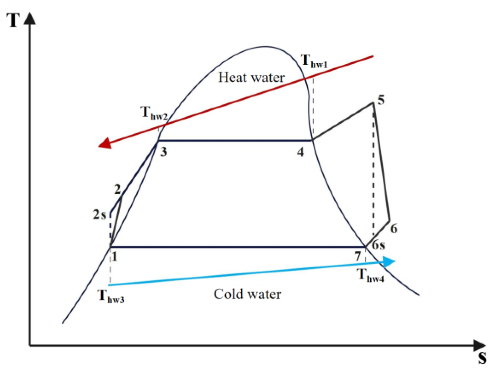
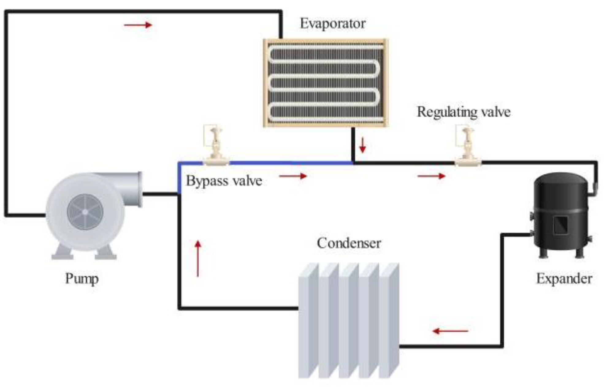
2.1. ORC System Description

In this paper, we chose a basic ORC system for waste heat recovery. The four main parts of a standard ORC system are the working fluid pump, expander, condenser, and evaporator, which together complete the work process. Its temperature–entropy (T-s) diagram is shown in Figure 1. The unsaturated liquid organic working fluid in process 2-5 becomes superheated after absorbing heat from the heat source in the evaporator. Then, the working fluid in processes 5-6 enters the expander, expands, and produces work. The overheated organic working fluid in the 6-1 process becomes a saturated liquid working fluid after passing through the condenser and dissipating system heat to the cold source. In the end, the pump presses it into the evaporator inlet, which is the 1-2 process. The dotted lines at 5-6s and 1-2s represent the ideal expansion and compression processes, respectively. The 2s and 6s points are the ideal state points. The open ORC system has a larger output power, but the closed ORC system has a higher thermal efficiency. In this paper, we selected an open ORC system as the working type.

2.2. Working Fluids

According to the above research, seven substances were selected as working fluids of the ORC system, as shown in

Table 1. Properties of 7 kinds of working fluids.

Name	M	Tcrit/°C	Pcrit/MPa	ODP-GWP	Tbp/°C	Ttp/°C	Safety a
R245fa	134	154.01	3.651	0-790	15.14	−102.1	B1
R114	171	145.68	3.257	0.85-4	3.59	−92.5	A1
R123	153	183.68	3.662	0.02-77	27.82	−107.15	B1
R601a	72	187.20	3.378	0-20	27.83	−160.5	A3
R601	72	196.55	3.370	0-20	36.06	−129.68	A3
R141b	117	204.35	4.212	0.086-0.15	32.05	−103.47	A1
R113	187	214.06	3.392	0.9-1.55	47.59	−36.22	A1

^a Refrigerant safety group classification. 1: No flammability; 2: Lower flammability; 3. Higher flammability; A: Lower toxicity; B: Higher toxicity.

. The output power and system efficiency of the seven working fluids under different heat source temperatures, different condensation temperatures, and different evaporation pressures were calculated by MATLAB R2016b-Refprop, as shown in Figure 2. As can be seen from the figure, R114 and R245fa obtained a higher output power under the set working conditions, because they had a critical temperature [26] that was relatively close to the heat source temperature, which conformed to the law. However, the system efficiency was relatively low, while R141b was the opposite. For every 1 °C increase in the heat source temperature, the difference between the maximum and minimum output powers of the different working fluids increased by an average of 46.44%, while the difference in the system efficiency only increased by 0.007%, and the maximum difference in the output power was 24.69 kW. Therefore, the working fluid with a larger system output power was preferred. Although R114 had lower toxicity than R245fa, it was eliminated due to cost, ozone layer depletion, and other issues. Therefore, R245fa was selected as the working fluid for the system in this paper.

2.3. Operating Conditions

The performance of the evaporator and system will be impacted to some extent by the presence of an evaporator pinch point temperature difference as well as the adaption of the heat source temperature and the evaporation temperature. The basic input operating parameters are shown in

Table 2. The basic input operating parameters.

Parameter	Value	Unit
vcw	0.2	m/s
Tcw	20	°C
Pcw	1000	kPa
Phw	1000	kPa
mhw	10	kg/s
Tair	25	°C
Tsh	5	K
Tsc	0	K
ΔTp	10	K
nexp	1500	r/min
Dexp	0.3556	m
ηpump	0.7	–
Thw_initial	125	°C
Tc_initial	45	°C

.

2.4. Model Assumptions and Construction

The following simplified assumptions were made about the model:

(1)

Assuming that there is equal heat exchange between the working medium side and the water side, the heat loss is not taken into account.

(2)

The flow pressure drop in the condenser is ignored, that is, the momentum equation is not considered.

(3)

The steady flow satisfies the mass equation (continuity equation), only considering the energy equation.

(4)

The mass flow rate at each position in the heat exchanger remains unchanged.

The following steps were included in the model’s construction process:

(1)

Under the initial design values in Table 2, calculate and obtain the initial value of the evaporation pressure when the expander output power is maximum, which was 827.46 kPa.

(2)

Calculate the pressure drop and actual heat exchange area of the heat exchanger, then select the appropriate type from the 12 brazed plate heat exchangers provided by the manufacturer [48].

(3)

Establish the range of changing working conditions through the self-regulation of the thermal parameters like the heat transfer coefficient and mass flow rate, etc., based on the structural and thermal parameters of the chosen heat exchanger type. The altering rules of the parameters under various working conditions were therefore obtained.

The structural parameters of the selected heat exchanger are shown in

Table 3. The structural parameters of the selected heat exchanger.

Parameter	Value	Unit
Single board channel volume	0.86	L
Maximum water flow rate	203	m3/h
Plate thickness	0.0004	m
Board spacing	0.0023	m
Effective heat exchange area of a single plate	0.45	m2
Single channel cross-sectional area	0.0014	m2
Process length	0.63	m
Plate width	0.42	m
Number of installed boards in the evaporator	41	–
Number of installed boards in the condenser	80	–

.

2.5. Mathematical Model

2.5.1. Heat Exchanger

Aspen plus-EDR was used to generate and draw a simple structural diagram of the heat exchanger, as shown in Figure 3.

The evaporator heat load is

$$Q_r=C\times q_r\times (h_5-h_2)$$

(1)

(1)

Water volume flow

$$V_{hw}=m_{hw\_in}\times 3600/{\rho }_{hw}$$

(2)

(2)

Number of flow channels and heat exchange area

$$n_e=V_{hw}/(s_e\times u_{hw}\times 3600)$$

(3)

$$A_{total}=(2\times n_e-1)\times f_e$$

(4)

(3)

Working fluid pressure drop and phase area ratio

(1) Two-phase area

Gas- and liquid-phase working fluid flow rates:

$$u_{rl,rg}=m_r\times (1-x_m)/(n_e\times {\rho }_{rl,rg}\times s_e)$$

(5)

Reynolds number of the gas- and liquid-phase working fluid:

$${\mathrm{Re}}_{rl,rg}=u_{rl,rg}\times d_e/{\upsilon }_{rl,rg}$$

(6)

Friction coefficients along the liquid phase and gas phase:

$$\left\{\begin{array}{l}{f}_{rl}=38/{\mathrm{Re}}_{rl}, f_{rg}=38/{\mathrm{Re}}_{rg} ({\mathrm{Re}}_{rl}\le 1000, {\mathrm{Re}}_{rg}\le 1000, C_2=5)\\ f_{rl}=38/{\mathrm{Re}}_{rl}, f_{rg}=1.22/{\mathrm{Re}}_{rg} ({\mathrm{Re}}_{rl}\le 1000, {\mathrm{Re}}_{rg}>1000, C_2=12)\\ f_{rl}=38/{\mathrm{Re}}_{rl}, f_{rg}=1.22/{\mathrm{Re}}_{rg} ({\mathrm{Re}}_{rl}>1000, {\mathrm{Re}}_{rg}\le 1000, C_2=10)\\ f_{rl}=1.22/{\mathrm{Re}}_{rl}, f_{rg}=1.22/{\mathrm{Re}}_{rg} ({\mathrm{Re}}_{rl}\le 1000, {\mathrm{Re}}_{rg}\le 1000, C_2=10)\end{array}\right.$$

(7)

The respective proportions of the three-phase areas:

$$l_{etp,esc,esh}=\mathsf{\Delta }{h}_{etp,esc,esh}/\mathsf{\Delta }{T}_{etp,esc,esh}$$

(8)

$$c_{etp,esh,esc}=l_{etp,esh,esc}/(l_{etp}+l_{esc}+l_{esh})$$

(9)

Length of each phase area:

$$L_{esc,esh,etp}=c_{esc,esh,etp}\times L_e$$

(10)

Liquid- and gas-phase pressure drops:

$$\mathsf{\Delta }{P}_{rl,rg}=\left(4\times f_{rl,rg}\times L_{etp}\times u_{rl,rg}^2\right)\times {10}^{-3}/\left(2\times d_e\right)$$

(11)

Martinelli parameters:

$$X_e=\sqrt{{\displaystyle \frac{\mathsf{\Delta }{\mathrm{P}}_{rl}}{\mathsf{\Delta }{P}_{rg}}}}$$

(12)

The square of the liquid-phase coefficient of friction: (C₂ = 12)

$${\phi }_{rl}^2=1+C_2/X_e+1/X_e^2$$

(13)

Pressure drop in the two-phase area:

$$\mathsf{\Delta }{P}_{etp}=1.25\times \mathsf{\Delta }{P}_{rl}\times {\phi }_{rl}$$

(14)

(2) Supercooled zone and superheated zone

Flow resistance coefficient:

$$\left\{\begin{array}{l}{\lambda }_{esc,esh}=0.3164\times {\mathrm{Re}}_{esc,esh}^{-0.25} ({\mathrm{Re}}_{esc,esh}>1000)\\ {\lambda }_{esc,esh}=64/{\mathrm{Re}}_{esc,esh} ({\mathrm{Re}}_{esc,esh}\le 1000)\end{array}\right.$$

(15)

Pressure drop:

$$\mathsf{\Delta }{P}_{esc,esh}={\lambda }_{esc,esh}\times L_{esc,esh}\times {\rho }_{esc,esh}\times u_{esc,esh}^2\times {10}^{-3}/\left(2\times d_e\right)$$

(16)

(3) Total pressure drop of the working fluid

$$\mathsf{\Delta }{P}_{etotal}=\mathsf{\Delta }{P}_{esc}+\mathsf{\Delta }{P}_{esh}+\mathsf{\Delta }{P}_{etp}$$

(17)

(4)

Heat transfer coefficient of water

$$N{u}_{hw}=0.023\times {\mathrm{Re}}_{hw}^{0.8}\times {\mathrm{Pr}}_{hw}^{0.3}$$

(18)

$${\alpha }_{hw}=N{u}_{he}\times K_{hw}/d_e$$

(19)

$$q_{hw1}={\alpha }_{hw}\times (T_{hw\_m}-T_{w\_e})$$

(20)

$$R_w={\delta }_e/K_w$$

(21)

Working fluid side wall temperature:

$$T_{w\_re}=T_{w\_e}-q_1\times R_w$$

(22)

(5)

Convection heat transfer coefficient on the working fluid side

$${\mathrm{Re}}_{etp}=m_r\times \left\{(1-x_m)+x_m\times \sqrt{{\displaystyle \frac{{\rho }_{rl}}{{\rho }_{rg}}}}\right\}\times {\displaystyle \frac{d_e}{{\mu }_{rl}}}$$

(23)

Nusselt number in the two-phase region:

$$\left\{\begin{array}{l}N{u}_{etp}=5.03\times {\mathrm{Pr}}_{le}^{1/3}\times {\mathrm{Re}}_{etp}^{1/3}({\mathrm{Re}}_{etp}<50000)\\ N{u}_{etp}=5.03\times {\mathrm{Pr}}_{le}^{1/3}\times {\mathrm{Re}}_{etp}^{0.8}({\mathrm{Re}}_{etp}\ge 50000)\end{array}\right.$$

(24)

Convection heat transfer coefficient on the working medium side:

$${\alpha }_{tp\_rside}=N{u}_{etp}\times K_{le}/d_e$$

(25)

Total flow heat transfer coefficient on the working fluid side:

$${\alpha }_r={\alpha }_{sc\_rside}\times c_{esc}+{\alpha }_{sh\_rside}\times c_{esh}+{\alpha }_{tp\_rside}\times c_{etp}$$

(26)

The heat transfer amount on the working fluid side was calculated based on the temperature difference between the wall surface and the working fluid:

$$q_r={\alpha }_r\times (T_{w\_re}-T_{r\_me})$$

(27)

Water side heat transfer coefficient:

$${\alpha }_{hw}=0.135\times {\mathrm{Re}}_{hw}^{0.73}\times {\mathrm{Pr}}_{hw}^{0.43}\times {({\displaystyle \frac{{\mathrm{Pr}}_{hw}}{{\mathrm{Pr}}_w}})}^{0.25}$$

(28)

Water side pressure drop:

$$\mathsf{\Delta }{P}_{hw}=1843\times {\mathrm{Re}}_{hw}^{-0.25}\times {\rho }_{hw}\times u_{hw}^2\times {10}^{-3}$$

(29)

(6)

Boiling heat transfer coefficient on the working fluid side

$$X_{pb}={\left({\displaystyle \frac{G_l}{G_g}}\right)}^{0.9}\times {\left({\displaystyle \frac{{\rho }_g}{{\rho }_l}}\right)}^{0.5}\times {\left({\displaystyle \frac{{\mu }_l}{{\mu }_g}}\right)}^{0.1}$$

(30)

Correction coefficient: (C₂ = 21)

$$F={\phi }_{pb}^{0.89}$$

(31)

Pool boiling heat transfer coefficient:

$${\alpha }_{pb}=0.00142\times \left({\displaystyle \frac{{\lambda }_l^{0.79}\times C_{pl}^{0.45}\times {\rho }_l^{0.49}\times g_c^{0.25}}{{\sigma }^{0.5}\times {\mu }_l^{0.29}\times r^{0.24}\times {\rho }_l^{0.24}}}\right)\times \mathsf{\Delta }{t}^{0.24}\times \mathsf{\Delta }{p}^{0.75}$$

(32)

(7)

Total working fluid side heat transfer coefficient

$${\alpha }_{r\_total}={\alpha }_{pb}+{\alpha }_{tp\_side}$$

(33)

(8)

Total heat transfer coefficient of the evaporator

$$K_e={({\displaystyle \frac{1}{{\alpha }_{r\_total}}}+{\displaystyle \frac{1}{{\alpha }_{hw}}}+1.0\times {10}^{-5}+{\displaystyle \frac{\delta }{\lambda }})}^{-1}$$

(34)

(9)

Logarithmic mean temperature difference

$$\mathsf{\Delta }{T}_{\log }={\displaystyle \frac{\mathsf{\Delta }{t}_{\max }-\mathsf{\Delta }{t}_{\min }}{\ln \frac{\mathsf{\Delta }{t}_{\max }}{\mathsf{\Delta }{t}_{\min }}}}$$

(35)

(10)

Actual heat exchange area

$$A_e=Q_r/(K_e\times \mathsf{\Delta }{T}_{\log })$$

(36)

The principles, methods, and calculating model and evaporator model are essentially the same and will not be described in detail here. The primary distinction is that in the condenser, the working fluid releases heat to the cooling water and condenses and transfers heat from the gas-phase working fluid to the liquid-phase working fluid. Therefore, what needed to be calculated was the condensation heat transfer coefficient. The formula is the following:

$${\alpha }_c={(1.47\times 1.25\times K_{lc}^3\times {\rho }_{lc}^2\times 1.27\times {10}^8/{\mu }_{lc}^2)}^{1/3}\times {\mathrm{Re}}^{-1/3}$$

(37)

2.5.2. Expander

The expander model mainly calculates the expander efficiency through the characteristic ratio, φ_exp, thereby obtaining the actual outlet enthalpy of the expander. The enthalpy difference and mass flow rate were used to obtain the output work and inlet specific volume. The calculation is the following:

$${\varphi }_{\exp }={\displaystyle \frac{\pi \times n_{\exp }\times D_{\exp }}{\sqrt{2\times (h_{\exp \_in}-h_{\exp \_out})}}}$$

(38)

$${\eta }_{\exp }=0.001\times {\varphi }_{\exp }^4-0.0075\times {\varphi }_{\exp }^3+0.0279\times {\varphi }_{\exp }^2-0.0373\times \varphi +0.8511$$

(39)

$$V_{\exp }=C\times v_5\times m_r\times 3600$$

(40)

$$W_{\exp }=m_r\times (h_{\exp \_in}-h_{\exp \_out})$$

(41)

2.5.3. Pump

The input and output status points of the pump in the actual ORC system are rather close together, and its efficiency has very little effect on the system computation [49]. Hence, it was enough to set the working fluid pump efficiency to a fixed value and perform thermal calculations to obtain the system efficiency.

Head:

$$H_{pump}=P_{pump\_out}/{\rho }_{pump\_in}$$

(42)

Volume flow:

$$V_{pump}=C\times v_{pump\_in}\times m_r\times 3600$$

(43)

Output work:

$$W_{pump}=m_r\times (h_{pump\_in}-h_{pump\_out})$$

(44)

2.5.4. System

$${\eta }_{sys}={\displaystyle \frac{W_{\exp }-W_{pump}}{Q_r}}$$

(45)

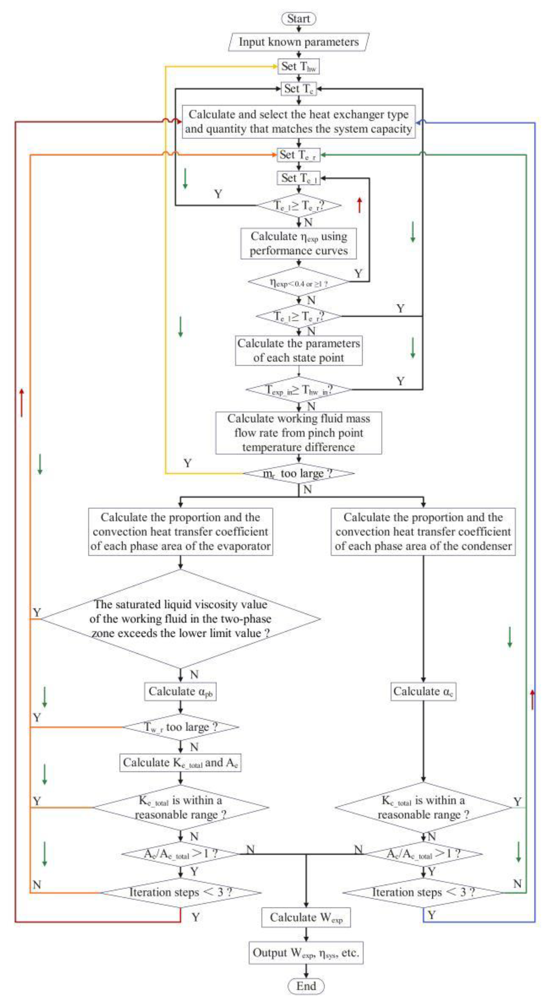
3. Algorithmic Logic Construction

An ORC system is difficult and expensive to construct because of its many relevant parameters, complicated shifting trends, serious component coupling errors, and nonlinear parameter correlation. When conditions do not allow, the numerical simulation of the system can grasp the changing rules of the system parameters and offer a sensible and useful guide for building experimental benches [50,51,52]. Parameters were separated into two categories in this paper: internal parameters and external parameters. External parameters are those that are external to a unit and are directly adjustable, whereas internal parameters are those that are present inside the unit cycle and cannot be directly changed. From the actual work process, when the system operating conditions changes, the external parameters, like the heat source water and the cooling water, can generally be directly altered. In addition to understanding the linear relationship between external parameters and core parameters, it is necessary to understand the linear relationship between some key internal parameters of a system to establish a logically correct mathematical model [53,54]. In this way, the relationship between these parameters can be used to construct a simplified model that makes sense and is better suited for the real work process when creating a feedback adjustment model of changing external parameters.

The actual ORC system consists of two parts: a main loop and a bypass loop. The heat source valve is opened initially, and when heat source water enters, the evaporator’s liquid level drops. After that, the pump is turned on, with the liquid level controlling its frequency. Next, the evaporator pressure progressively increases while the heat source valve position is kept open. The working fluid now completes the cycle via the bypass valve rather than passing through the host. As illustrated in Figure 4, after the pressure reaches an appropriate level, the main engine’s regulating valve should be gradually opened to raise speed and establish grid connection.

3.1. System Sensitivity Analysis

The sensitivity analysis model mainly includes variable evaporation pressure and condensation temperature system models, calculated by MATLAB. Both models follow the same essential steps. Variable evaporation pressure was used as an example in the following introductory analysis, which consisted of the following steps:

(1)

Define the target parameters.

(2)

Determine the input parameters.

(3)

Preliminarily give the range of variable evaporation pressures:

(1)

Lower the limit of the interval. In order to ensure that the temperature difference or pressure difference in the system drives heat conversion, the lower limit setting value of the evaporation pressure cannot be lower than or equal to the condensation pressure value.

(2)

Since the mass flow rate is iteratively obtained by setting the pinch point temperature difference value, and taking into account the critical parameters of the working fluid, there are initially two judgment conditions for the upper limit value:

a. The evaporation pressure is generally set to about 5 kPa lower than the critical pressure.

b. Assuming that the evaporator does not have any heat exchange, the temperature of the heat source water at the pinch point temperature difference is the heat source water inlet temperature. As of right now, the evaporation temperature value is the difference between the heat source water inlet temperature and the evaporator pinch point temperature difference. This value is the upper limit value. Since the heat source water inlet temperature and the pinch point temperature difference are both settable parameters, the upper limit value is modified each time the set value fluctuates.

c. It is not possible to continuously raise the evaporation pressure due to changes in other parameters. These need to be located by running multiple sets of working conditions during program operation and debugging.

(4)

Ascertain the quantity and content of judgment conditions based on the parameters that may cause errors and require debugging under the aforementioned fundamental presumptions. Apart from modifying the variable interval, the set input parameter values are subject to the following constraints:

(1) The heat source water temperature cannot be increased endlessly as an input value. The maximum heat load of the heat exchanger or the actual heat exchange area must be taken into consideration. Having too high of a heat source water temperature and flow rate can exceed the heat exchanger load and fail to converge.

(2) Considering that the evaporation pressure value is too high, the temperature value of the working fluid at the evaporator outlet is equal to or higher than the heat source temperature value.

(3) The heat transfer coefficient of the heat exchanger limits the upper limit of the interval.

(4) The difference in temperature between the saturated gaseous point of the working fluid and the corresponding water temperature of the heat source is too small due to an excessively high condensation temperature or evaporation pressure. To begin the procedure, a fair initial value must be chosen; if the issue still exists after a given number of iterations, the interval’s upper limit must be decreased.

(5)

Establish calculating models for each component.

(6)

Determine the output parameters and curves of the system.

(7)

Perform program debugging.

The algorithm logic diagram of the system sensitivity analysis is shown in Figure 5.

3.2. System Steady-State Adjustment

The actual operation of the ORC system usually requires stable or less fluctuating power generation output, that is, the output power must fluctuate less. The output power is obtained by multiplying the enthalpy difference between the inlet and outlet of the expander and the mass flow rate of the working fluid. The mass flow rate of the working fluid varies with the pump rotating speed. Both the pump frequency and the mass flow rate need to essentially stay the same after the system is operating steadily.

This led to the conclusion that the mass flow rate and the expander output power had tiny fluctuation errors, which was the system’s model constraint condition. The mass flow rate rises as the temperature of the heat water rises and falls as the evaporation pressure rises [55,56,57,58,59]. The algorithmic constraint conditions were modified based on how these relationships changed in MATLAB, as shown in Figure 6.

4. Results and Discussion

This paper focused on analyzing the performance variations in a BPE and its impact on the system, since the system parameters were directly related to the thermal characteristics of the evaporator. By calculating the output power W_exp of five points at a 5 °C pinch point temperature difference, the relative error between the model calculation value and the literature [60] value did not exceed 5%, and the system model was well verified, as shown in Figure 7.

4.1. Variable Working Condition Parameters and Interval Ranges

The obtained variable working condition parameters and interval ranges are shown in

Table 4. (a) Working conditions with the variable P_e. (b) Working conditions with the variable T_c. (c) Steady adjustment of the ORC system with the variable T_{hw_in}.

(a)
Parameter	Value	Unit
Thw_in	125	°C
Tc	45	°C
Interval ranges of Pe	600–1410	kPa
(b)
Parameter	Value	Unit
Thw_in	125	°C
Te	104	°C
Interval ranges of Tc	28–48	°C
(c)
Parameter	Value	Unit
Wexp	153.11	kW
mr	9.09	kg/s
Interval ranges of Thw_in	125–137	°C

.

4.2. Variable Evaporation Pressure

Figure 8 shows the change rule for each phase area ratio in the evaporator with P_e. With increasing evaporation pressure, the saturation temperature increases. It boils more easily and more bubbles form in the evaporator. At the same time, saturated gaseous working fluid also becomes more superheated. That is the reason why the ratio of the two-phase zone and superheated zone gradually rises. The two-phase zone represented the biggest share, increasing from 70.22% to 75.83%. The supercooled zone followed, decreasing from 27.56% to 20.72%. With the smallest percentage, the superheated zone rose from 1.53% to 3.44%.

The heat flux and mass flow rate have a direct impact on the heat transfer coefficient. Bubbles form more quickly when the heat flux rises. An increase in the mass flow rate expedites the removal of bubbles produced in the evaporator and promotes convective heat transfer. Consequently, the heat transfer coefficient increases. All of that can be seen in Figure 9. The values for the heat transfer coefficient, mass flow rate, and heat flux were 2264.65–3230.40 W/(m²·K), 3.14–11.55 kg/s, and 14.04–46.32 kW/m², respectively.

As Figure 10b illustrates, the mass flow rate of the working fluid decreased when the evaporation pressure increased. From the previous analysis, a drop in the mass flow rate can cause bubbles to deposit, which makes the utilization ratio of two heat exchangers decrease, as shown in Figure 10a. Among them, the evaporator utilization ratio decreased from 74.85% to 38.32% and the condenser utilization ratio decreased from 66.61% to 13.69%.

The output power of the expander is the product of the mass flow rate and the enthalpy difference between the inlet and outlet. The latter increases with evaporation pressure. When the evaporation pressure was less than 827.46 kPa, the increase in specific enthalpy difference was greater than the decrease in the mass flow rate, so the output power showed an increasing trend. The impact of mass flow on the output power started to outweigh the specific enthalpy difference when the evaporation pressure rose over 827.46 kPa, resulting in a decrease in output power. As a result, the output power had a maximum value of 153.11 kW. The system efficiency was 7.78% and mass flow rate was 9.13 kg/s when the output power reached its maximum.

As the evaporation pressure rises, the heat transfer amount of the evaporator is the product of the heat transfer coefficient, heat transfer area, and temperature difference. The decrease in the heat transfer coefficient and actual heat exchange area lead to the decrease in the heat transfer amount in the evaporator.

System efficiency is the ratio of the net output work to the evaporator heat transfer. Taking the evaporation pressure of 827.46 kPa as the boundary, its value increased because the heat transfer amount decreased and the net output power increased on the left side of it. While on the right side, the system efficiency increased because the decrease in the heat exchange amount was greater than the decrease in the output power of the expander. The system efficiency ranged from 5.74 to 11.04%.

4.3. Variable Condensation Temperature

First of all, it can be seen from Figure 13b that the mass flow rate was calculated by the evaporator model and was thus less susceptible to variations in the condensation temperature. It increases slightly as the condensation temperature rose and its average value was 3.36 kg/s, which was essentially stable.

The curve of evaporator-phase zone ratio, varying with the condensation temperature, is presented in Figure 11. The increase in the condensation temperature makes the inlet temperature of the evaporator increase, which leads to the supercooled zone decreasing. The tiny increase in the two-phase zone and superheated zone mainly occurs because the mass flow rate slightly increases. From the figure, the ratio of the two-phase zone increased from 74.91% to 75.81% and the superheated zone increased from 3.28% to 3.32%. The ratio of the supercooled zone decreased from 21.80% to 20.87%.

The data above show that the mass flow rate varied relatively little, indicating that the heat flow rate had the greatest impact on the evaporator heat transfer coefficient. As the condensation temperature increased, the evaporator inlet specific enthalpy and temperature increased, and the inlet and outlet specific enthalpy difference and heat transfer temperature difference decreased, resulting in a decrease in the evaporator heat load. However, the increase in the temperature of the working fluid side helped to increase the generation rate of bubbles, thus raising the heat transfer coefficient. As shown in Figure 12, when the heat flux increased from 52.83 kW/m² to 63.94 kW/m², the heat transfer coefficient increased from 1721.31 W/(m²·K) to 2374.77 W/(m²·K).

It can be seen from Figure 13a that, as the condensation temperature increased, the evaporator utilization ratio dropped from 70.56% to 51.91%, and the condenser utilization ratio dropped from 95.94% to 45.71%. This is because the heat transfer coefficient of the evaporator decreased, so the heat exchange process was suppressed. Therefore, the actual heat exchange area of the evaporator decreased; phase change heat can bring greater heat transfer benefits. The two-phase process of the condenser accounted for the largest proportion, which was reduced from 90.7% to 80.5%. The decrease in the proportion of the two-phase zone weakened the phase heat transfer process inside the condenser, which made its actual heat exchange area be reduced, resulting in a decrease in the utilization ratio.

The parameters of the system are presented in Figure 13b. The system efficiency dropped from 13.64% to 10.43%, and the expander output power dropped from 116.95 kW to 80.60 kW. As the condensation temperature increases, the specific enthalpy at the outlet of the expander increases, and the specific enthalpy difference between the inlet and outlet of the expander decreases. In addition, the mass flow rate decreases. Therefore, the output power showed a downward trend. From the above analysis, it can be seen that although the heat exchange amount of the evaporator decreased, the decrease in the output power was much greater than the decrease in the heat exchange amount in the evaporator, resulting in a continuous decline in system efficiency. Based on analysis from the perspective of system physics principles, the increase in the condensation temperature caused the total heat exchange temperature difference in the system to decrease, resulting in a continuous decline in system efficiency.

4.4. Steady-State Regulation

Figure 14 shows system and heat exchange parameter variation curves with the heat source temperature. The evaporation pressure increased from 814.46 kPa to 1136.46 kPa, the condensation temperature from 294.46 kPa to 412.01 kPa, and the system efficiency from 7.83% to 7.95%. This is because as the heat source temperature rises, the output power generation will fluctuate. To balance the fluctuations, it is necessary to adjust the changes in two parameters, which are the mass flow rate and the specific enthalpy difference between the inlet and outlet of the expander. The mass flow rate increases with a heat source temperature increase. The increase in evaporation pressure causes the heat transfer temperature difference in the evaporator to decrease, which can weaken the increase in the mass flow rate. This can simulate a basic change in the mass flow caused by the constant pumping power in the actual process.

After balancing out the fluctuations in mass flow, the increase in evaporation pressure increases the specific enthalpy difference between the inlet and outlet of the expander, resulting in output power fluctuations. Then, the condensation pressure decreases, which decreases the specific enthalpy difference to reduce the fluctuation in output power. The increase in the system temperature difference leads to an increase in the system efficiency. Among them, for every 1 °C increase in the heat source water temperature, the evaporation pressure increased by 26.83 kPa, an increase of 3.29%; the condensation pressure increased by 9.79 kPa, an increase of 3.32%; and the system efficiency increased by 1.2%.

Increases in the evaporation pressure and heat source temperature increase the overall temperature of the evaporator, which cause the working fluid to shift to a more superheated state. Since the increase in condensation temperature is smaller than the increase in the evaporation pressure, the supercooled zone proportion increases. The two-phase zone proportion decreased from 69.65% to 67.82%, the supercooled zone proportion increased from 28.70% to 30.12%, and the superheated zone proportion increased from 1.86% to 2.06%. These changing rules are shown in Figure 15.

Figure 16 presents the linear relationship between the heat transfer coefficient, mass flow rate, and heat flux in the evaporator. The mass flow rate was kept constant, so the heat transfer coefficient was mainly affected by the heat flux. As the heat flux increased from 59.40 kW/m² to 65.80 kW/m², the heat transfer coefficient increased from 2776.07 W/(m²·K) to 2992.74 W/(m²·K). This part of the results was mentioned before, so we will not go into much more detail.

5. Conclusions

Variable working condition parameters in ORC systems are typically derived from design values, artificial givens, or experiments, without taking into account their correlations with the operating parameters in the model. Analyzing the performance changes in the system based on the performance parameter changes in the heat exchangers is insufficient. In addition, a model perspective of the system control solution is absent from the steady-state control of the system when the heat source varies. In order to solve the above problems, this paper included the following working steps:

• A system model for the application scenario of a 100–200 kW ORC system with BPHEs was designed.
• A sensitivity analysis of the system was carried out based on the performance changes in the heat exchangers.
• To make sure the system could continue to produce a steady power output even when the heat source’s temperature fluctuated, an adjustment strategy and modeling computation were proposed.
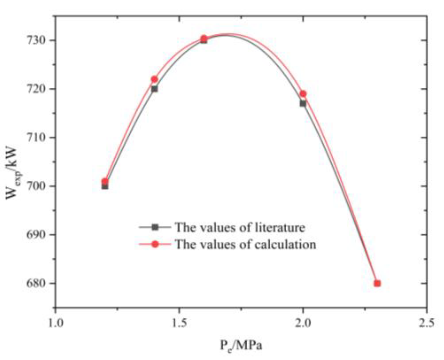
• The model results were compared and verified with the results of the R245fa-ORC experimental test papers, which provided a foundation for the design and practical application of the ORC system.

The main results were the following:

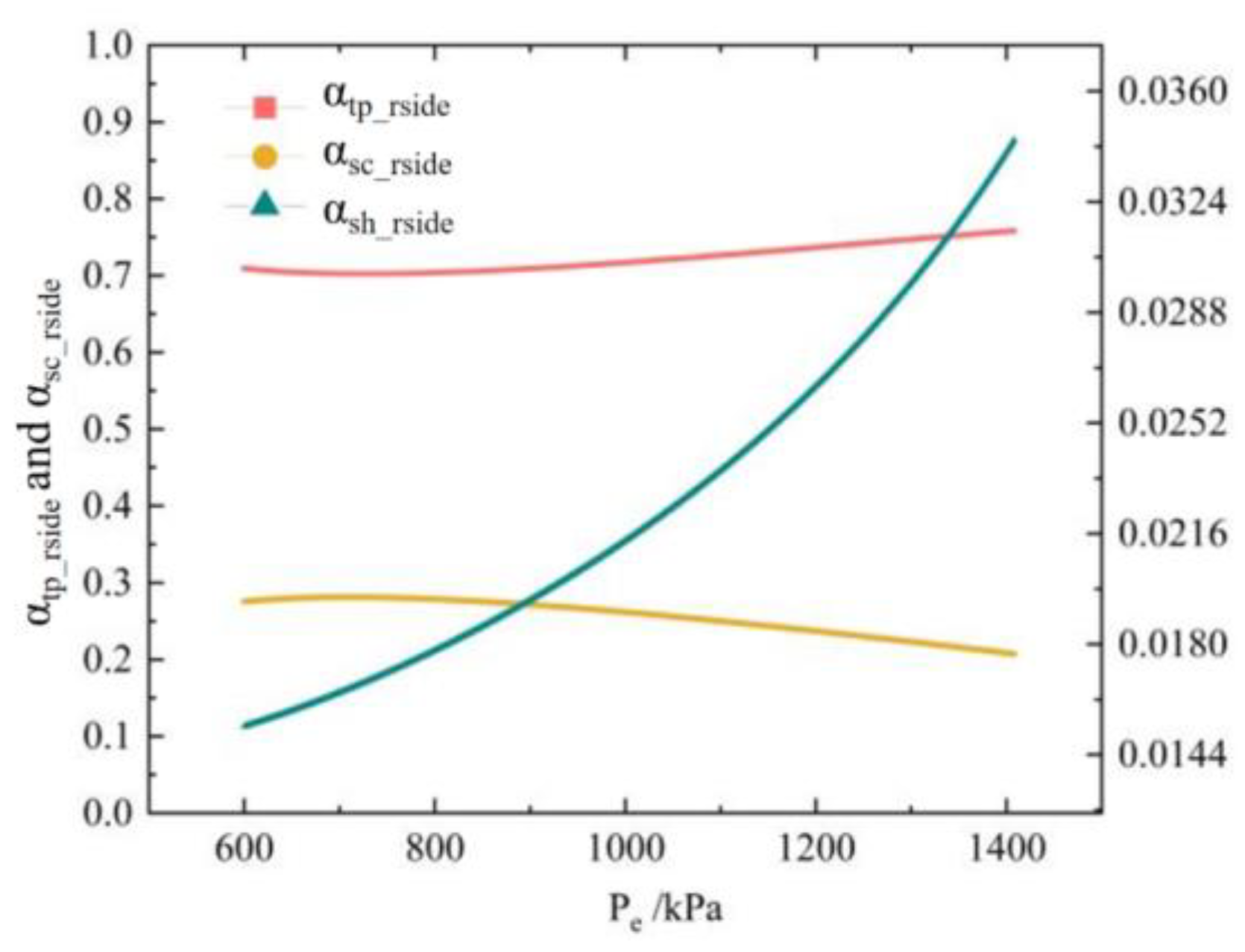
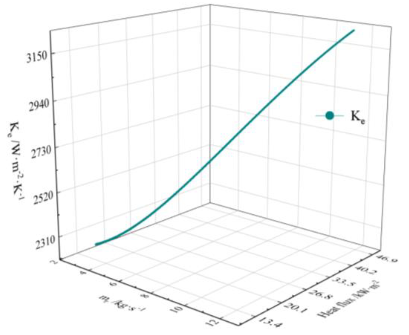
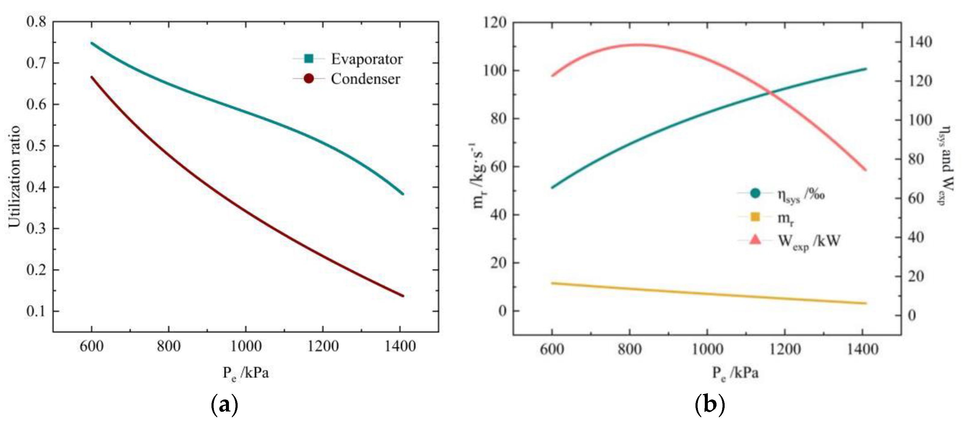
• When the heat source temperature was 125 °C and the condenser temperature was 45 °C, as the evaporation pressure increased from 600 to 1410 kPa, the two-phase zone in the evaporator accounted for the largest proportion, increasing from 70.22% to 75.83%. The supercooled zone followed, decreasing from 27.56% to 20.72%. The superheated zone, which accounted for the smallest proportion, increased from 1.53% to 3.44%. The decrease in the mass flow rate and heat flux made the heat transfer coefficient decrease from 46.32 kW/m² to 14.04 kW/m². The evaporator utilization ratio decreased from 74.85% to 38.32% and the condenser utilization ratio from 66.61% to 13.69%. The output power had a maximum value of 153.11 kW. When the output power reached its maximum, the system efficiency was 7.78% and the mass flow rate was 9.13 kg/s. The system efficiency increased from 5.74 to 11.04%.
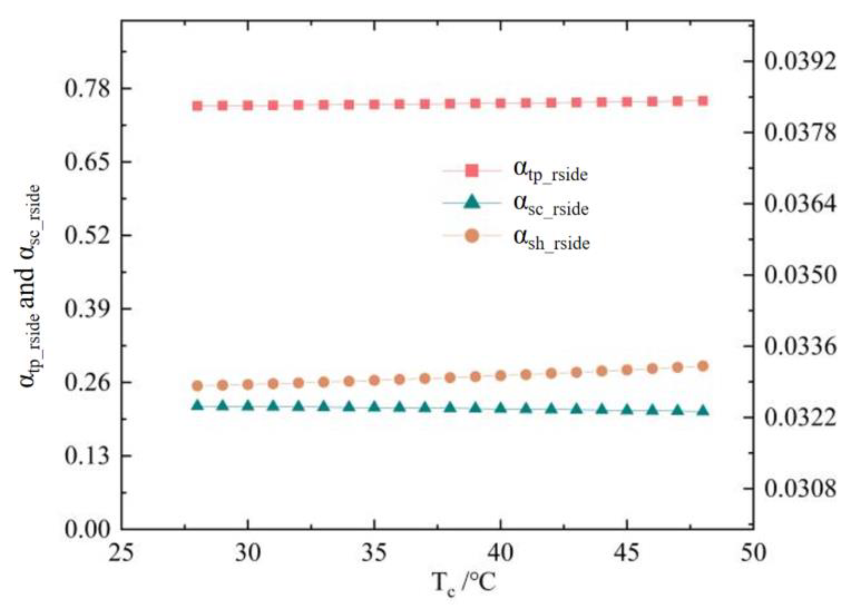
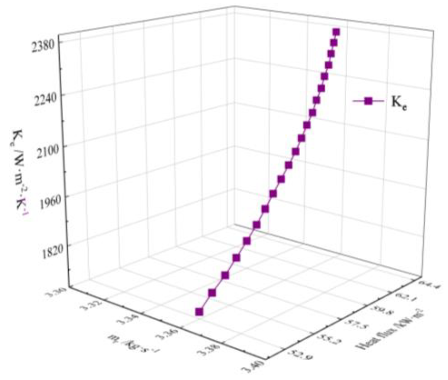
• When the heat source temperature was 125 °C and evaporation temperature was 104 °C, the increase in the condensation temperature from 28 to 48 °C made the mass flow rate have a tiny increase of 0.02% and an average value of 3.36 kg/s. The two-phase zone and superheated zone slightly increased from 74.91% to 75.81% and from 3.28% to 3.32%, respectively. The ratio of the supercooled zone decreased from 21.80% to 20.87%. The heat flux increased from 52.83 kW/m² to 63.94 kW/m², while the heat transfer coefficient increased from 1721.31 W/(m²·K) to 2374.77 W/(m²·K). The evaporator utilization ratio dropped from 70.56% to 51.91%, and the condenser utilization ratio dropped from 95.94% to 45.71%. The system efficiency dropped from 13.64% to 10.43%, and the expander output power dropped from 116.95 kW to 80.60 kW.
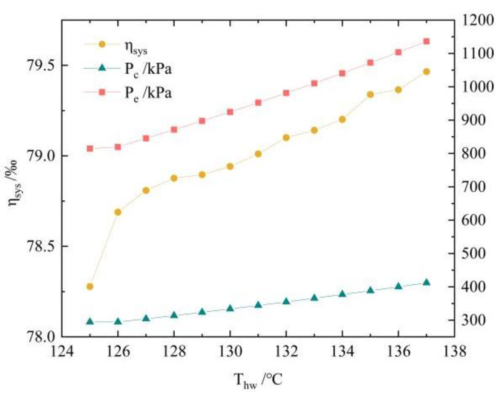
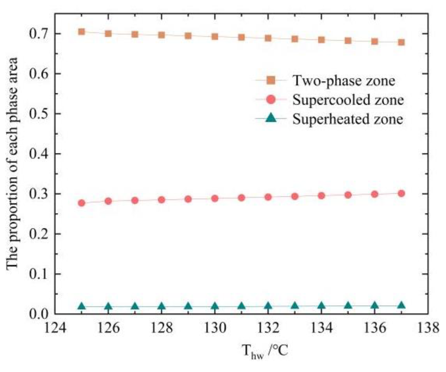
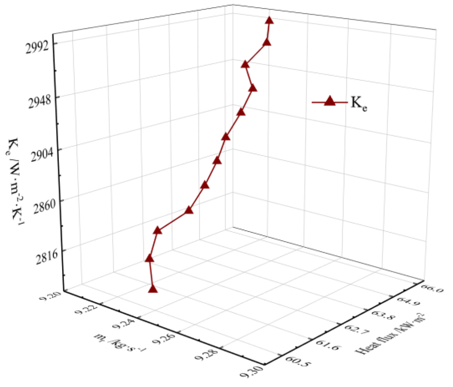
• When the heat source temperature increased, fluctuations in power generation were produced. The was in order to balance out these fluctuations and simulate the law that the mass flow rate was controlled by the working fluid pump and remained basically unchanged during actual stable operation. The evaporation pressure increased from 814.46 kPa to 1136.46 kPa, while the condensation temperature increased from 294.46 kPa to 412.01 kPa. System efficiency increased from 7.83% to 7.95%. At this time, in the BPE, the two-phase zone proportion decreased from 69.65% to 67.82%, the supercooled zone proportion increased from 28.70% to 30.12%, and the superheated zone proportion increased from 1.86% to 2.06%. The heat transfer coefficient increased from 2776.07 W/(m²·K) to 2992.74 W/(m²·K) as the heat flux increased.

These research results can provide a reasonable and effective reference for the design and practical application of an ORC system. In future research, the matching of different types of heat exchangers with system operating conditions can be considered, and testing and supplemental experimental data also need to be complemented. Improving the comparative analysis of condensers is also one of the important research directions of this work that need to be improved.

References

1. Thurairaja, K.; Wijewardane, A.; Jayasekara, S.; Ranasinghe, C. Working Fluid Selection and Performance Evaluation of ORC. Energy Procedia 2017, 156, 244–248. [Google Scholar] [CrossRef]
2. Mao, L.F.; Peng, H.; Zhao, J.W.; Hu, B.S. Generator Selection and Design of Grid-connected for ORC Power System. Energy Conserv. Technol. 2017, 35, 71–74. [Google Scholar]
3. Tang, H. Research on Twin-Screw Expander Characteristics and Organic Rankine Cycle System Performance. Ph.D. Thesis, Xi’an Jiaotong University, Xi’an, China, 2016. [Google Scholar]
4. Xing, C.D.; Peng, X.; Guo, R.L.; Zhang, H.G.; Yang, F.B.; Yu, M.Z.; Yang, A.R.; Wang, Y. Machine learning-based multi-objective optimization and thermodynamic evaluation of organic Rankine cycle (ORC) system for vehicle engine under road condition. Appl. Therm. Eng. 2023, 231, 120904. [Google Scholar] [CrossRef]
5. Li, T.L.; Wang, Q.L.; Zhu, J.L.; Hu, J.L.; Fu, W.C. Thermodynamic optimization of organic Rankine cycle using two-stage evaporation. Renew. Energy 2015, 75, 654–664. [Google Scholar] [CrossRef]
6. Mago, P.J.; Srinivasan, K.K.; Chamra, L.M.; Somayaji, C. An examination of exergy destruction in organic Rankine cycles. Int. J. Energ. Res. 2008, 32, 26–38. [Google Scholar] [CrossRef]
7. Tchanche, B.F.; Lambrinos, G.; Frangoudakis, A.; Papadakis, G. Exergy analysis of micro-organic Rankine power cycles for a small scale solar driven reverse osmosis desalination system. Appl. Energy 2010, 87, 306–1295. [Google Scholar] [CrossRef]
8. Yamamoto, T.; Furuhata, T.; Arai, N.; Mori, K. Design and testing of the Organic Rankine Cycle. Energy 2001, 26, 239–251. [Google Scholar] [CrossRef]
9. Hou, S.Y.; Zhou, Y.D.; Yu, L.J.; Zhang, F.Y.; Cao, S.; Wu, Y.D. Optimization of a novel cogeneration system including a gas turbine, a supercritical CO2 recompression cycle, a steam power cycle and an organic Rankine cycle. Energy Convers. Manag. 2018, 172, 457–471. [Google Scholar] [CrossRef]
10. Wang, W.; Deng, S.; Zhao, D.P.; Zhao, L.; Lin, S.; Chen, M.C. Application of machine learning into organic Rankine cycle for prediction and optimization of thermal and exergy efficiency. Energy Convers. Manag. 2020, 210, 112700. [Google Scholar] [CrossRef]
11. Wei, D.; Lu, X.; Lu, Z.; Gu, J. Dynamic modeling and simulation of an organic Rankine cycle (ORC) system for waste heat recovery. Appl. Therm. Energy 2008, 28, 1216–1224. [Google Scholar] [CrossRef]
12. Feng, X. Theoretical Research on Low-Temperature Waste Heat Power Generation System in Organic Rankine Cycle. Master’s Thesis, Shanghai Jiaotong University, Shanghai, China, 2011. [Google Scholar]
13. Zhar, R.; Allouhi, A.; Jamil, A.; Lahrech, K. A comparative study and sensitivity analysis of different ORC configurations for waste heat recovery. Case Stud. Therm. Eng. 2021, 28, 101608. [Google Scholar] [CrossRef]
14. Fan, G.L.; Gao, Y.J.; Ayed, H.; Marzouki, R.; Aryanfar, Y.; Jarad, F.; Guo, P.X. Energy and exergy and economic (3E) analysis of a two-stage organic Rankine cycle for single flash geothermal power plant exhaust exergy recovery. Case Stud. Therm. Eng. 2021, 28, 101554. [Google Scholar] [CrossRef]
15. Wang, J.L.; Zhao, L.; Wang, X.D. A comparative study of pure and zeotropic mixtures in low-temperature solar Rankine cycle. Appl. Therm. Energy 2010, 87, 66–73. [Google Scholar] [CrossRef]
16. Hung, T.C.; Shai, T.Y.; Wang, S.K. A review of organic Rankine cycles (ORCs) for the recovery of low-grade waste heat. Energy 1997, 22, 7–661. [Google Scholar] [CrossRef]
17. Pedro, J.M.; Louay, M.C.; Kalyan, S.; Chandramohan, S. An examination of regenerative organic Rankine cycles using dry fluids. Appl. Therm. Energy 2008, 28, 998–1007. [Google Scholar]
18. Chacartegui, R.; Sanchez, D.; Munoz, J.M.; Sanchez, T. Alternative ORC bottoming cycles for combined cycle power plants. Appl. Energy 2009, 86, 662–670. [Google Scholar] [CrossRef]
19. Rayegan, R.; Tao, Y.X. A procedure to select working fluids for solar Organic Rankine Cycles (ORCs). Renew. Energy 2011, 36, 659–670. [Google Scholar] [CrossRef]
20. Yu, W.; Ban, X.; Liu, C.; Li, Q.B.; Xin, L.Y.; Huang, Z.Y.; Wang, S.K. Experimental and Theoretical Study on the Thermal Stability and Pyrolysis Mechanism of Octamethyltrisiloxane (MDM) with Lubricating Oil. J. Anal. Appl. Pyrolysis 2024, 179, 106521. [Google Scholar] [CrossRef]
21. Liu, Y.; Jing, Y.; Liu, C. Heat Capacity of Liquid Octamethyltrisiloxane (MDM) and Hexamethyldisiloxane (MM): Measurement and Molecular Dynamics Study. J. Mol. Liq. 2024, 404, 124937. [Google Scholar] [CrossRef]
22. Yu, W.; Liu, C.; Tan, L.; Li, Q.B.; Xin, L.Y.; Wang, S.K. Thermal Stability and Thermal Decomposition Mechanism of Octamethyltrisiloxane (MDM): Combined Experiment, ReaxFF-MD and DFT Study. Energy 2023, 284, 129289. [Google Scholar] [CrossRef]
23. Yang, L.; Gong, M.; Guo, H.; Dong, X.Q.; Shen, J.; Wu, J.F. Effects of Critical and Boiling Temperatures on System Performance and Fluid Selection Indicator for Low Temperature Organic Rankine Cycles. Energy 2016, 109, 830–844. [Google Scholar] [CrossRef]
24. Zhai, H.; An, Q.; Shi, L. Analysis of the Quantitative Correlation Between the Heat Source Temperature and the Critical Temperature of the Optimal Pure Working Fluid for Subcritical Organic Rankine Cycles. Appl. Therm. Eng. 2016, 99, 383–391. [Google Scholar] [CrossRef]
25. Ye, Z.; Yang, J.; Shi, J.; Chen, J. Thermo-economic and Environmental Analysis of Various Low-GWP Refrigerants in Organic Rankine Cycle System. Energy 2020, 199, 117344. [Google Scholar] [CrossRef]
26. Özcan, Z.; Ekici, Ö. A Novel Working Fluid Selection and Waste Heat Recovery by An Exergoeconomic Approach for a Geothermally Sourced ORC System. Geothermics 2021, 95, 102151. [Google Scholar] [CrossRef]
27. Sylvain, Q.L.; Lemort, V.; Lebrun, J. Experimental study and modeling of an Organic Rankine Cycle using scroll expander. Appl. Energy 2010, 87, 1260–1268. [Google Scholar]
28. Kane, H.E. Intégration et Optimisation Thermoéconomique and Environomique de Centrales Thermiques Solaires Hybrides. Ph.D. Thesis, Laboratoire d’ Energétique Industrielle, Ecole Polytechnique Fédérale de Lausanne, Lausanne, Switzerland, 2002. [Google Scholar]
29. Qi, F.L. Experimental Research and Simulation of Organic Rankine Cycle; North China Electric Power University: Beijing, China, 2017. [Google Scholar]
30. Zhang, Y.; Wu, Y.; Xia, G.; Ma, C.; Ji, W.; Liu, S.; Yang, K.; Yang, F. Development and experimental study on organic Rankine cycle system with single-screw expander for waste heat recovery from exhaust of diesel engine. Energy 2014, 77, 499–508. [Google Scholar] [CrossRef]
31. Ni, J.X. Analysis to the Dynamic Performance with Variable Conditions and Simulation to Organic Rankine Cycle. Master’s Thesis, Tianjin University, Tianjin, China, 2017. [Google Scholar]
32. Tchanche, B.F.; Lambrinos, G.; Frangoudakis, A.; Papadakis, G. Low-grade heat conversion into power using organic Rankine cycles-A review of various applications. Renew. Sustain. Energy Rev. 2011, 15, 3963–3979. [Google Scholar] [CrossRef]
33. Manente, G.; Toffolo, A.; Lazzaretto, A.; Paci, M. An Organic Rankine Cycle off-design model for the search of the optimal control strategy. Energy 2013, 58, 97–106. [Google Scholar] [CrossRef]
34. Calise, F.; Capuozzo, C.; Carotenuto, A.; Vanoli, L. Thermoeconomic analysis and off-design performance of an organic Rankine cycle powered by medium-temperature heat sources. Sol. Energy 2014, 103, 595–609. [Google Scholar] [CrossRef]
35. Calise, F.; D’Accadia, M.D.; Macaluso, A.; Piacentino, A.; Vanoli, L. Exergetic and exergoeconomic analysis of a novel hybrid solar-geothermal polygeneration system producing energy and water. Energy Convers. Manag. 2016, 115, 200–220. [Google Scholar] [CrossRef]
36. Shi, R.; He, T.; Peng, J.; Zhang, Y.; Zhuge, W. System design and control for waste heat recovery of automotive engines based on Organic Rankine Cycle. Energy 2016, 102, 276–286. [Google Scholar] [CrossRef]
37. Yang, X.L.; Huang, S.R.F.F.; Dai, W.Z. Analysis of thermal performance of heat source-regulated organic Rankine cycle power generation system. J. Eng. Therm. Energy Power 2017, 32, 34–40. [Google Scholar]
38. Bull, J.; Buick, J.M.; Radulovic, J. Heat exchanger sizing for organic Rankine cycle. Energies 2020, 13, 3615. [Google Scholar] [CrossRef]
39. Xu, J.; Luo, X.; Chen, Y.; Mo, S. Multi-criteria design optimization and screening of heat exchangers for a subcritical ORC. Energy Procedia 2015, 75, 1639–1645. [Google Scholar] [CrossRef]
40. Walraven, D.; Laenen, B.; D’haeseleer, W. Comparison of shell-and-tube with plate heat exchangers for the use in low-temperature organic Rankine cycles. Energy Convers. Manag. 2014, 87, 227–237. [Google Scholar] [CrossRef]
41. Chatzopoulou, M.A.; Lecompte, S.; Markides, N.C. Off-design optimisation of organic Rankine cycle (ORC) engines with different heat exchangers and volumetric expanders in waste heat recovery applications. Appl. Energy 2019, 253, 113442. [Google Scholar] [CrossRef]
42. Zhang, C.; Liu, C.; Wang, S.K.; Xu, X.X.; Li, Q.B. Thermo-economic comparison of subcritical organic Rankine cycle based on different heat exchanger configurations. Energy 2017, 123, 728–741. [Google Scholar] [CrossRef]
43. Hu, K.Y.; Zhu, J.L.; Li, T.L.; Zhang, W. R245fa Evaporation Heat Transfer and Pressure Drop in a Brazed Plate Heat Exchanger for Organic Rankine Cycle (ORC). In Proceedings of the World Geothermal Congress, Melbourne, Australia, 16–24 April 2015. [Google Scholar]
44. Longo, G.A.; Gasparella, A. Refrigerant R134a vaporisation heat transfer and pressure drop inside a small brazed plate heat exchanger. Int. J. Refrig. 2007, 30, 821–830. [Google Scholar] [CrossRef]
45. Tari, Z.G. Flow boiling heat transfer characteristics of R245fa refrigerant in a plate heat exchanger. J. Phys. Conf. Ser. 2020, 1599, 012007. [Google Scholar] [CrossRef]
46. Kim, D.Y.; Kim, K.C. Thermal performance of brazed metalfoam-plate heat exchanger as an evaporator for organic Rankine cycle. Energy Procedia 2017, 129, 451–458. [Google Scholar] [CrossRef]
47. Muhammad, I.; Muhammad, U.; Yang, Y.; Park, B.S. Flow boiling of R245fa in the brazed plate heat exchanger: Thermal and hydraulic performance assessment. Int. J. Heat Mass Transf. 2017, 110, 657–670. [Google Scholar]
48. Cheng, B.H.; Li, X.R.; Yao, R.Y. Plate Heat Exchanger and Heat Exchange Device Technical Application Manual; China Architecture & Building Press: Beijing, China, 2005. [Google Scholar]
49. Zhang, H.G.; Yang, Y.X.; Meng, F.X.; Zhao, R.; Tian, Y.M.; Liu, Y. Running performance of working fluid pump for organic Rankine cycle system. CIESC J. 2017, 68, 3573–3579. [Google Scholar]
50. Pei, G.; Wang, D.Y.; Li, J.; Li, Y.Z.; Ji, J. Experimental study on organic Rankine cycle combined heat and power system. CIESC J. 2013, 64, 1994–2000. [Google Scholar]
51. Hu, B.; Ma, W.B. Thermodynamic analysis of low-temperature geothermal refrigeration system based on organic Rankine cycle. Adv. New Renew. Energy 2014, 2, 122–128. [Google Scholar]
52. Shao, Y.J.; Jin, B.S.; Zhong, W.Q.; Hao, L. Modeling and performance analysis of micro organic Rankine cycle thermoelectric system. J. Southeast Univ. 2013, 43, 798–802. [Google Scholar]
53. Muhammad, I.; Muhammad, U.M.; Sik, P.B.; Yang, Y.M. Comparative assessment of Organic Rankine Cycle integration for low temperature geothermal heat source applications. Energy 2016, 102, 473–490. [Google Scholar]
54. Li, Y.R.; Wang, X.Q.; Li, C.C.; Wu, S.Y.; Liu, C. Performance analysis of a coupled transcritical and subcritical organic Rankine cycle. J. Eng. Thermophys. 2015, 36, 176–1181. [Google Scholar]
55. Roy, J.P.; Mishra, M.K.; Misra, A. Performance analysis of an organic Rankine cycle with superheating under different heat source temperature conditions. Appl. Energy 2011, 88, 2995–3004. [Google Scholar] [CrossRef]
56. Wei, D.H.; Lu, X.S.; Lu, Z.; Gu, J.M. Performance analysis and optimization of organic Rankine cycle (ORC) for waste heat recovery. Energy Convers. Manag. 2007, 48, 1113–1119. [Google Scholar] [CrossRef]
57. Weng, Y.W. Low Grade Heat Energy Conversion Processes and Their Utilizations; Shanghai Jiaotong University Press: Shanghai, China, 2014. [Google Scholar]
58. Twomey, B.; Jacobs, P.A.; Gurgenci, H. Dynamic performance estimation of small-scale solar cogeneration with an organic Rankine cycle using a scroll expander. Appl. Therm. Eng. 2013, 51, 1307–1316. [Google Scholar] [CrossRef]
59. Zhang, J.; Zhou, Y.; Wang, R.; Xu, J.L.; Fang, F. Modeling and constrained multivariable predictive control for ORC (Organic Rankine Cycle) based waste heat energy conversion systems. Energy 2014, 66, 128–138. [Google Scholar] [CrossRef]
60. Lin, Q.Y.; Wang, D.; Zhao, Y.Y. Impact analysis of key design parameters on ORC system performance. Turbine Technol. 2023, 65, 352–370. [Google Scholar]
Figure 1. T-s diagram of the ORC system.
Applsci 14 08728 g001
Figure 2. Working fluid calculation comparison.
Applsci 14 08728 g002
Figure 3. A simple structural diagram of the heat exchanger.
Applsci 14 08728 g003
Figure 4. The actual working process of the ORC system.
Applsci 14 08728 g004
Figure 5. The algorithmic logic diagram of the system sensitivity analysis.
Applsci 14 08728 g005
Figure 6. The algorithmic logic diagram of the system steady-state adjustment.
Applsci 14 08728 g006
Figure 7. Model validation.
Applsci 14 08728 g007
Figure 8. The curves of the evaporator-phase zone ratios varying with Pe.
Applsci 14 08728 g008
Figure 9. The linear relationship between the Ke, mr, and heat flux in the evaporator.
Applsci 14 08728 g009
Figure 10. The influence of Pe on the system and heat exchangers. (a) The utilization ratios of the heat exchangers. (b) Parameters of the system.
Applsci 14 08728 g010
Figure 11. The curves of the evaporator-phase zone ratios varying with Tc.
Applsci 14 08728 g011
Figure 12. The linear relationship between the Ke, mr, and heat flux in the evaporator.
Applsci 14 08728 g012
Figure 13. The influence of the condensation temperature on the system and heat exchangers. (a) The utilization ratios of the heat exchangers. (b) Parameters of the system.
Applsci 14 08728 g013
Figure 14. System and heat exchanger parameter variation curves with Thw.
Applsci 14 08728 g014
Figure 15. The curve of the evaporator-phase zone ratio varying with Thw.
Applsci 14 08728 g015
Figure 16. The linear relationship between the Ke, mr, and heat flux in the evaporator.
Applsci 14 08728 g016