Abstract
When considering agricultural commodity transaction data, long sampling intervals or data sparsity may lead to small samples. Furthermore, training on small samples can lead to overfitting and makes it hard to capture the fine-grained fluctuations in the data. In this study, a multi-scale forecasting approach combined with a Generative Adversarial Network (GAN) and Temporal Convolutional Network (TCN) is proposed to address the problems related to small sample prediction. First, a Time-series Generative Adversarial Network (TimeGAN) is used to expand the multi-dimensional data and t-SNE is utilized to evaluate the similarity between the original and synthetic data. Second, a greedy algorithm is exploited to calculate the information gain, in order to obtain important features, based on XGBoost. Meanwhile, TCN residual blocks and dilated convolutions are used to tackle the issue of gradient disappearance. Finally, an attention mechanism is added to the TCN, which is beneficial in terms of improving the forecasting accuracy. Experiments are conducted on three products, garlic, ginger and chili. Taking garlic as an example, the RMSE of the proposed method was reduced by 1.7% and 1% when compared to the SVR and RF models, respectively. Its accuracy was also improved (by 4.3% and 3.4%, respectively). Furthermore, TCN-attention and TCN were found to require less time compared to GRU and LSTM. The accuracy of the proposed method increased by about 5% when compared to that without TimeGAN in the ablation study. Moreover, compared with TCN, the Gated Recurrent Unit (GRU), and the Long Short-term Memory (LSTM) model in the multi-scale price forecasting task, the proposed method can better utilize small samples and high-dimensional data, leading to improved performance. Additionally, the proposed model is compared to the Transformer and TimesNet models in terms of its accuracy, deployment cost, and other metrics.
1. Introduction
With the globalization of the economy, the impacts of commodity price fluctuations have emerged as a significant concern in the context of sustainable socio-economic development. Yu-Yue Hu [1] proposed that when commodity prices rise too quickly, potential risks may arise in financial markets. Moreover, cost-driven inflation can occur, affecting the profits of small and medium-sized Enterprises in the midstream and downstream, which are intermediate links of the supply chain. Yukui Sun et al. [2] have reported that the accurate prediction of price fluctuations is beneficial with regard to risk management and helps in the pricing of downstream products. Meanwhile, the price fluctuation of agricultural products is related to the income of farmers and the living standard of residents and also has an impact on the stability of the social economy.
Regarding the actual transaction of bulk commodities, there exist small samples with short collection periods or sparse data recorded with low trading frequency. The use of such data for model training can lead to overfitting and makes it difficult to determine fine-grained changes in the process of price forecasting. Data augmentation is beneficial to monitor price fluctuations and provide insights for intelligent decision-making. Data augmentation is often used in image processing, such as translation, rotation, scaling, and other affine transformations. As for time-series data, geometric transformations are often adopted, as well as window cropping or the addition of noise in the time and frequency domains. There still exist shortcomings regarding the data analysis of the overall distribution characteristics [3]. Generative Adversarial Networks (GANs) can be utilized to generate data, such as T-CGAN, RCGAN, and so on. However, these methods face challenges related to parallelization, and it is necessary to further validate their generalization ability.
Forecasting algorithms commonly include statistical, machine learning (ML), deep learning (DL), and Integrated Learning methods, among others. Traditionally, statistical methods are based on linear structures and may not perform well on complex, multi-feature, and non-linear data. Machine learning approaches offer flexibility in feature correlation analysis, overfitting, and regularization techniques but face performance and accuracy bottlenecks when dealing with long time series. Deep learning approaches have the potential to reduce human involvement in feature engineering and enable the rapid perception of market changes. Small sample-based prediction poses difficulties related to capturing the intrinsic complex relationships among features and the regularity of distributions when using traditional algorithms.
Taking into account the above, the purpose of this research is not only to apply TimeGAN to augment the obtained data in order to prevent overfitting on sparse or small samples but also to reduce the runtime and computing costs. For this purpose, a multi-scale comparison method is proposed. The key contributions of this study are summarized as follows: (1) In the field of commodities, traditional machine learning methods often struggle with low prediction accuracy when using sparse and small sample data sets, whereas deep learning techniques are prone to overfitting. Our study mainly focuses on utilizing TimeGAN to augment the data and improving the training performance of the models.
(2) A multi-scale forecasting strategy is employed, which combines XGBoost with TCN-attention to predict the short-term price of agricultural commodities at daily and hourly levels. The proposed method is compared with the GRU, LSTM, and TCN algorithms in terms of computational cost, time, and accuracy. Additionally, the Transformer and TimesNet methods are also considered for comparison.
The experiment involves data augmentation of hourly and daily data for electronic trading or spot transactions. Moreover, the study compares the outcomes of price and volatility predictions obtained with different methods. The remainder of the paper is structured as follows: The related work on data augmentation and price forecasting is presented in Section 2. The methodologies of data augmentation, feature extraction, and TCN-Attention are described in Section 3. The experimental results of the proposed method, in comparison with those of TCN, GRU, LSTM, Transformer, and TimesNet models, are detailed in Section 4 and Section 5. Finally, Section 6 provides the Conclusions.
2. Literature Review
The related work is mainly presented in terms of two aspects: the methods of data augmentation and an overview of price prediction.
2.1. Data Augmentation
Zhao et al. [4] divided the approaches to small sample learning into three categories: model fine-tuning, data augmentation, and transfer learning. Data augmentation methods involve enhancing the features and expanding the target data sets with auxiliary data or information. Based on the learning method, they further categorized learning methods into three kinds: based on unlabeled data, data synthesis, and feature enhancement by data augmentation. Pan Y. et al. [5] have proposed a data augmentation method based on knowledge to monitor oil conditions using sparse and small samples. Furthermore, data augmentation was carried out using particle filtering algorithms after data decomposition. However, this method has a high computational complexity, and it may be hard to efficiently compute the solution. Li D. C. et al. [6] have put forward a noise-based spatial clustering method based on DBSCAN and AICc density for small sample clustering. It utilizes a Maximum P-Value method to estimate whether each sample distribution is unimodal or multimodal and creates virtual samples based on the sample distributions. Wang et al. [7] proposed generating virtual data to improve sample diversity. The method jointly trains the generation model and classification algorithms by means of an end-to-end strategy combined with meta-learning methods. Timestamps are used as an input in the T-CGAN method in order to handle irregular time intervals [8]. Hyland S. L. et al. have combined an RNN with GAN in RGAN and RCGAN to generate multi-dimensional time-series data; however, this method suffers from insufficient parallelization, and further validation of its generalization ability is required.
2.2. Price Forecasting
2.2.1. Statistical Methods
The price volatility is a crucial element in evaluating risk and determining the pricing of downstream commodities. Guangwei Shi [9] has noted that fluctuations in the trading prices of commodities often present characteristics such as a spiky thick-tailed distributions of returns, the aggregation of fluctuations, persistence, leverage effects, volatility spillover effects, and interdependence among higher-order error terms. Engle [10] introduced an Autoregressive Conditional Heteroskedasticity Model (ARCH) and applied this model to study the volatility of the U.K. inflation index. However, its limitation is that it treats positive and negative fluctuations as having the same impact on volatility and imposes strict parameter constraints. Bollerslev [11] proposed the Generalized Autoregressive Conditional Heteroskedasticity (GARCH) model based on the ARCH model, providing a more detailed description of asset volatility dynamics. The ARCH model can capture the interdependence between errors and describe the temporal aggregation and variation of time-series. It is frequently employed in the forecasting of financial asset volatility. Taylor [12] introduced the stochastic volatility model, which is capable of capturing abrupt changes in financial time-series.
The abovementioned models are primarily based on low-frequency data. Andersen et al. [13] put forth the realized volatility, which is applicable to high-frequency data for assessing price volatility. This method boasts ease of computation and non-parametric modeling characteristics. While the ARIMA model can predict non-stationary time-series and offers quick computation, its accuracy is compromised when the series presents higher volatility.
2.2.2. Machine Learning Methods
Traditional statistical methods are often built upon assumptions and still exhibit limitations when tasked with analyzing intricate non-linear data sets. In contrast, machine learning approaches offer superior flexibility in correlation analysis, dealing with overfitting and regularization, among other aspects. Jabeur et al. [14] harnessed the XGBOOST algorithm to forecast the price volatility of gold, followed by comparing its performance with six alternative machine learning models to confirm the efficacy of the algorithm. Valente [15] predicted high-frequency, multi-seasonal time-series data sets using a forward feature selection based on the SVR. Meanwhile, Shaolong Sun et al. [16] have integrated the Ensemble Empirical Mode Decomposition, Least Squares Support Vector Regression, and K-means clustering methods, which proved valuable in forecasting foreign exchange rates. Advancements in deep learning technology coupled with the better computational capabilities of hardware make it possible to reduce the need for manual intervention, process vast amounts of multi-source heterogeneous data concurrently, and rapidly perceive market exigencies.
2.2.3. Forecasting Methods Based on Deep Learning
Deep learning techniques have undergone significant advancements across various fields, which have empowered machines to grasp abstract concepts and enhance their capabilities in representational learning. Neural networks have emerged as universal frameworks for dealing with issues in multiple research fields. Wang et al. [17] proposed Recurrent Neural Network (RNNs), which are commonly employed for processing time-series data; however, they have issues with handling the gradient disappearance problem, long-term dependencies, and parallelization. In this regard, gating mechanisms can be utilized to mitigate gradient disappearance and better capture temporal dependencies in LSTM networks. Shaolong Sun [16] combined wavelet analysis with LSTM to develop financial time-series prediction models that overcome the challenges posed by complex features and non-linear correlations. Comparing LSTM and Gated Recurrent Units (GRUs), the latter exhibit faster convergence due to their fewer number of parameters. Furthermore, CNNs offer efficient parallel data processing, and one-dimensional convolutions can be substituted for RNNs in sequence modeling. Liu Suhui [18] has exploited a deep learning model combined with news event data for stock price prediction. Moreover, a convolutional neural network based on event information was established using a text representation in the form of event triples and an attention mechanism. The WaveNet model, introduced by Oord et al. [19], serves as an autoregressive probabilistic model. It employs extended causal convolutions and has been used in audio generation, time-series prediction, and machine translation. Bai et al. [20] introduced the TCN for processing time-series data. Cao et al. [21] developed a discrete dynamic model, utilizing TCN to compute the conditional probabilities for different kinds of stocks. Meanwhile, attention mechanisms can be added to capture the time-varying distribution. As for graph convolutional neural networks, Wei et al. [22] introduced the Spectral Temporal Graph Neural Network (StemGNN) model, which exploits the Graph Fourier Transform (GFT) and Discrete Fourier Transform (DFT) to transform the spatio-temporal domain into the frequency domain, effectively capturing time–space dependencies. Cheng et al. [23] proposed the Multimodal Graph Neural Network (MAGNN) for financial forecasting, which integrates intra-modal graph attention and inter-modal attention mechanisms, providing a solution to crucial issues related to financial price forecasting.
Duan Z. et al. [24] introduced CauGNN, a model that incorporates neural Granger causal graphs to delineate causal relationships among multiple variables. Lim B. et al. [25] provided an overview of time-series forecasting based on deep learning. Their work focused on the evolution of hybrid deep models that integrate statistical models with neural networks. Wen Q. et al. [26] discussed the performance of Transformer models in handling time-series data, including assessments of robustness, model dimensions, and seasonal trend decomposition. Zhou H. [27] supposed that the limitations of Transformers (e.g., quadratic time complexity and high memory consumption) hinder their direct application to long-term time-series prediction. Wu H. et al. [28] introduced Autoformer based on a deep decomposition architecture and an autocorrelation mechanism, which is an intricate forecasting model for long-term time series that can decompose intricate time series into manageable elements. Next, Informer was used to mitigate the time complexity of the model, handle lengthy sequences, and improve the inference speed. Wu H. et al. [29] proposed the extension of one-dimensional sequences into a multi-period 2D tensor and encapsulated changes in intra- or inter-periodic variations into rows and columns of the tensor. The algorithm’s efficacy covers short- and long-term time-series prediction, a filling task, classification, and anomaly detection. Fanling Huang et al. [8] introduced TCGAN, a convolutional approach that is designed for time-series classification and clustering. The solution is particularly exploited to handle challenges associated with the shortage of labeled data and imbalanced sample distributions. Furthermore, Zhang C. et al. [30] investigated four deep time-series generation methods for commodity markets and compared them with classical probabilistic models. As a result, they proposed a data-driven approach to commodity risk management. The key characteristics of various methods are detailed in Table 1.

Table 1.
The key characteristics of various methods.
We previously published a paper [31] in which the XGBoost and TCN-attention methods were applied for the short-term forecasting of power load, incorporating influencing factors such as weather, exchange rate, and electricity consumption, among others. This approach is considered generalizable and was further extended to tackle small sample prediction issues. During the research, it was found that data of seasonal commodities typically present a small sample size and long data-collection intervals, prompting us to conduct further exploration. In another study [32], we combined XGBoost with TCN-attention for cotton price forecasting, incorporating nine influencing factors, including the supply and demand relationship, the exchange rate, macroeconomics, and the industrial chain. We examined the impacts of multiple factors on agricultural product prices. However, this study focused on small-sample forecasting using real data from the Peony International Trading Market in which factors such as weather and exchange rate are treated as static data.
Finally, while TimeGAN has been typically used for data augmentation in engineering applications, its use in the financial field has been limited. Therefore, this study focuses on integrating the TimeGAN method with TCN-attention to forecast short-term prices across multiple scales, with an emphasis on assessing the model’s usability.
3. Principles of Price Forecasting Combined with GAN
This study focuses on utilizing TimeGAN to generate data for small samples of agricultural products. Meanwhile, similarity evaluation is used to assess the difference between the generated data and the original data. Furthermore, the XGBoost method is utilized to extract important features, followed by price prediction using a TCN-attention network.
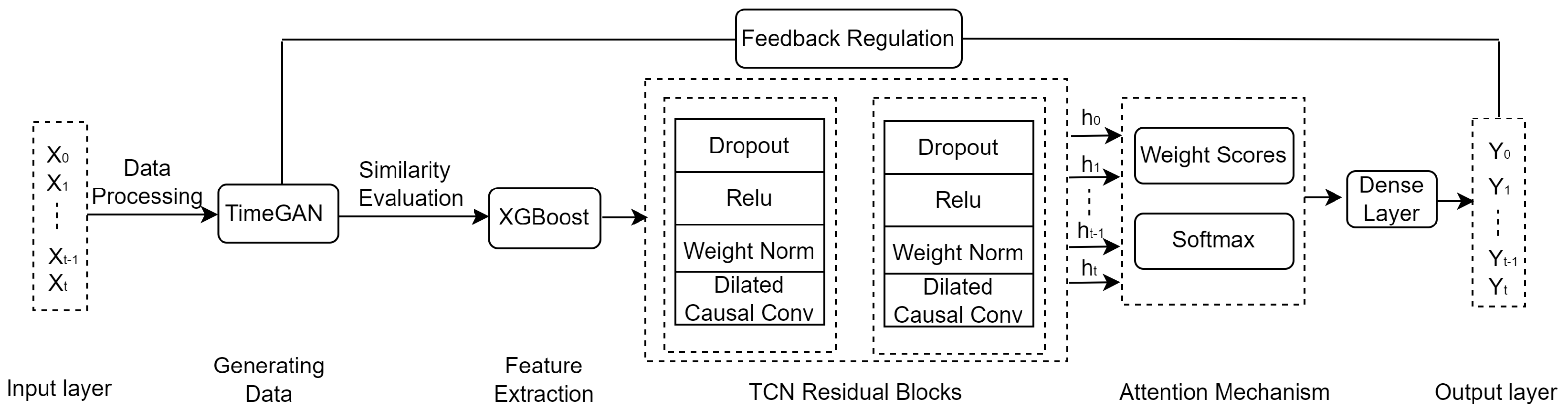
The price forecasting model is composed of an input layer, data generation, feature extraction, TCN Residual Blocks, an attention mechanism, and an output layer, as shown in Figure 1.
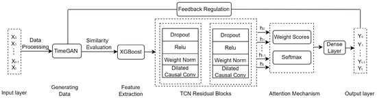
Figure 1.
Framework of price forecasting.
Step 1: Multi-dimensional data of agricultural products (e.g., garlic or ginger) are used as input. Data pre-processing mainly deals with the original data using a sliding window method and includes excluding outliers, filling missing values, and other processes.
Step 2: New data are generated using the TimeGAN framework [33], and a dual-scale measurement approach is used to evaluate the quality of the generated data. To measure the proximity between the generated and original data, the t-distributed Stochastic Neighbor Embedding (t-SNE) method and a visualization approach are utilized.
Step 3: Correlation analysis among features is carried out, exploiting XGBoost to extract important features.
Step 4: TCN residual blocks and dilated convolution are leveraged to reduce the processing time for long sequences. Meanwhile, an attention mechanism is used to improve the forecasting accuracy.
Step 5: Three groups of agricultural product data are used for experimentation in order to compare the predictive outcomes of the proposed model at multiple scales with those obtained using LSTM, GRU, TCN, Transformer, and TimesNet models. A comparative analysis is conducted by evaluating metrics such as R-squared (), Root Mean Squared Error (RMSE), and so on.
During model training, small samples can lead to the overfitting of deep learning models, while they may result in lower prediction accuracy of machine learning methods. TimeGAN can capture correlations between time series to generate highly similar data. Therefore, it is utilized in this study to increase the data volume, with the aim of improving model performance. Important features are extracted using XGBoost, which helps to reduce the computational complexity. A dilated convolutional network can compute data across time steps in parallel, thus capturing long-term dependencies with fewer parameters. Therefore, it is employed for price forecasting and is found to converge fasterthan the GRU and LSTM models.
3.1. Data Generation
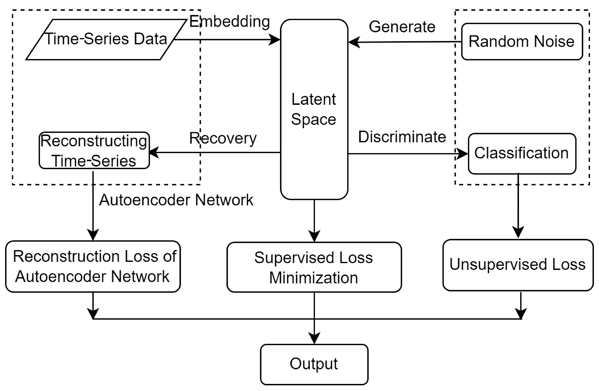
TimeGAN can generate time-series data that retain the intricate temporal dynamics inherent to the original data. It merges the adaptability of the unsupervised GAN framework with the controllability of supervised learning using autoregressive models. The TimeGAN model mainly encompasses four components—the Embedding Network, the Recovery Network, the Generator, and the Discriminator—as illustrated in Figure 2.

Figure 2.
TimeGAN framework.
The Embedding Network serves a crucial purpose, namely, establishing an invertible mapping between features and feature representations of the latent layer, which contributes to reducing the dimensionality of data in an adversarial learning space. The embedding function is shown in Equation (1):
where the feature spaces are denoted by and , while the corresponding latent vector spaces are represented by and respectively. S represents the static features , whereas indicate temporal features in the time-series. The tuples conform to a certain joint distribution P, where T is a random variable. Meanwhile, are instantiated as , and the set X contains n feature vectors, where . Here, s represents the high-dimensional static eigenvectors of trading data, indicates the mapped low-dimensional static eigenvectors, represents the high-dimensional temporal eigenvectors at time t, represents the low-dimensional temporal eigenvectors at time t, and e is the embedding function implemented via recurrent networks. The training data set is denoted as .
The recovery function reconstructs the original high-dimensional static and temporal features from the low-dimensional feature vectors of the data. The recovery function is represented as shown in Equation (2):
where and serve as the recovery Embedding Networks for the static and temporal embeddings, respectively; represents the recovered high-dimensional static feature vector; and represents the recovered high-dimensional temporal feature vector at time t.
The loss function for the embedding and recovery functions during the construction of the low-dimensional feature space for the data and recovery of the high-dimensional feature space is shown in Equation (3):
The output results of the Generator, along with the low-dimensional feature vectors from the embedded functions, are inputted into the Discriminator through joint encoding, as illustrated in Equation (4). For the purpose of generating data, it is necessary to enter the output of the Generator into the Discriminator. We have
where and represent the static and temporal vector spaces for known distributions, respectively; and are random noise, where is sampled from a Gaussian distribution and follows the Wiener process; and denote the generated static feature vectors and temporal feature vectors, respectively; and g is a generating function. Furthermore, is a generative network for static features and is a recurrent Generator for temporal features.
The Discriminator compares the output generated data with real transaction data in order to determine whether the generative data closely resemble real data in order to obtain classification results. Hence, we have
The Discriminator function d is implemented by a bi-directional recurrent network with a feed-forward output layer, where and are the output layer classification functions and represents the synthetic output. The unsupervised joint loss function for the Generator and Discriminator is denoted as , as shown in Equation (6):
where and correspond to the classification results of the static and temporal features of real data, respectively, while and denote those of synthetic data; and indicate the classification results for the static and temporal features, which include real or synthetic transaction data; and the synthetic data follow the probability distribution .
The supervised loss is minimized through joint training of the embedded and generative networks, as shown in Equation (7):
The optimization loss function for TimeGAN is expressed in Equation (8):
where and are hyperparameters and the weight parameter sets for the embedded network, Recovery Network, Generator, and Discriminator network are denoted as , , , and , respectively.
3.2. Quality Assessment of t-SNE
For the t-SNE algorithm [34], a similarity matrix is established according to the likeness among data points existing in a high-dimensional space. The matrix lays the foundation for constructing a conditional probability distribution. In essence, the distribution quantifies the likelihood that other points are chosen as neighbors for a given data point.
Subsequently, the similarity distribution allows for the construction of relationships among points in a lower-dimensional space. Meanwhile, the proximity of data points in the space has an effect on assigned probabilities: the closer the distance, the higher the probability.
The t-SNE method exploits the minimization of the Kullback–Leibler (KL) divergence to make the similarity distribution in the low-dimensional space as close as possible to the conditional probability distribution of the high-dimensional space. The steps are described as follows.
Step 1: The data in the high-dimensional space are mapped into in the low-dimensional space, which are then visually represented using a scatter plot. For each point in the high-dimensional space, the probability distribution of the similarity between and is denoted as , as shown in Equation (9):
where denotes the variance of the Gaussian distribution centered around . A probability distribution, with a fixed degree of complexity set by the user, is achieved by a bisection search process for [35].
Step 2: The joint probability density function is calculated for high-dimensional samples, as shown in Equation (10):
Step 3: The low-dimensional data are initialized as .
Step 4: A Student’s t-distribution with a single degree of freedom is employed as the heavy-tailed distribution in the low-dimensional graph. The joint probability in the lower-dimensional space is defined as shown in Equation (11):
The similarity between the distributions of the high- and low-dimensional spaces is computed according to the Kullback–Leibler (KL) divergence. The gradient descent method is used to minimize the cost function, while the gradient is computed as illustrated in Equation (12):
where the cost function C is calculated according to the KL divergence: .
Step 5: A large momentum term is added into the gradient in order to avoid becoming trapped in a local minimum, thus accelerating optimization. The output is updated as shown in Equation (13):
where signifies the solution obtained in iteration , denotes the learning rate, and m() denotes the momentum factor at iteration .
Step 6: Iteratively execute Steps 4 and 5 until the cost function tends to convergence.
3.3. Important Feature Extraction
The feature importance can be evaluated using the average information gain, average coverage, or feature split counts [35] in the XGBoost algorithm. This study utilizes a greedy algorithm [36] to calculate the information gain of multiple features in order to perform feature extraction. The principle is described as follows.
The objective function consists of the loss function and the regularization term shown in Equations (14) and (15), respectively:
where and are penalty coefficients, denotes the number of leaves, and is the L2 norm of the leaf scores.
In the loss function , is an observed value, the predicted value of the sample is , and represents the predicted value of the first trees to the sample.
The first-order partial derivative and the second-order partial derivative are computed based on the second-order Taylor expansion of the loss function. Let , , where refers to the sample set on the leaf node.
The information gain before and after node splitting is shown in Equation (16), where and stand for the before- and after-split minima of the objective function, respectively, and l and r represent the left and right subtrees, respectively.
Variable gain refers to the maximum information gain among various splits based on a specific eigenvalue. For the purpose of calculating feature importance in the model, the gains of each tree need to be summed, and the gain proportion of a given feature with respect to the entire model must be computed.
3.4. Price Forecasting Based on TCN-Attention Principle
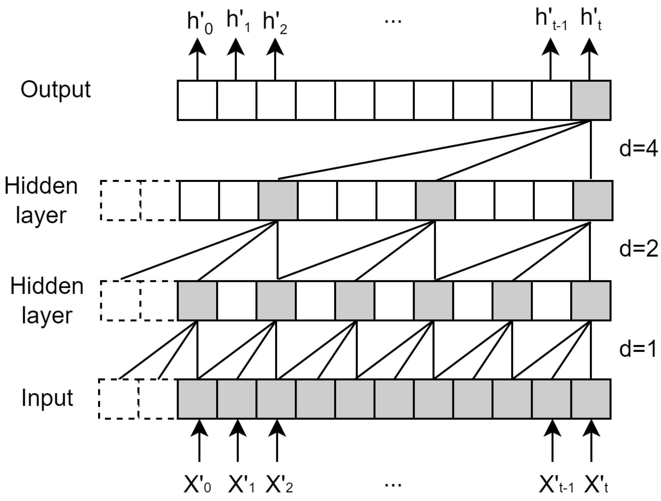
The vector (,…,,) derived from XGBoost is utilized as the input for TCN. Let , and (t) be an output vector. The hidden layer of TCN is padded in order to maintain consistency in length, matching that of the input layer. The ranges of receptive fields mainly depend on the network depth (n), the size of the convolution kernel (k), and the dilation factor (d), as shown in Figure 3.
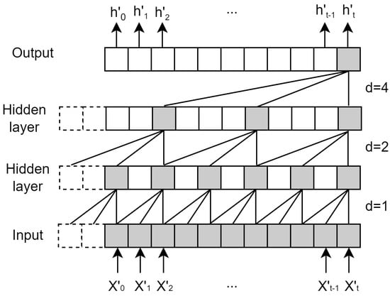
Figure 3.
The principle of TCN.
In Equation (17), F() represents a convolution operation on the sequence element .
supposing that we have a filter , and where denotes the direction of the past. From the input layer to the output layer, the higher the layer, the larger the receptive field. Residual blocks are exploited to deal with the degradation issue in the TCN algorithm. The residual blocks consist of double-layer networks, including dilated causal convolution, weight normalization, and activation function (e.g., ReLU). Meanwhile, convolution is used to enable elements to be added with tensors of the same shape [19,20].
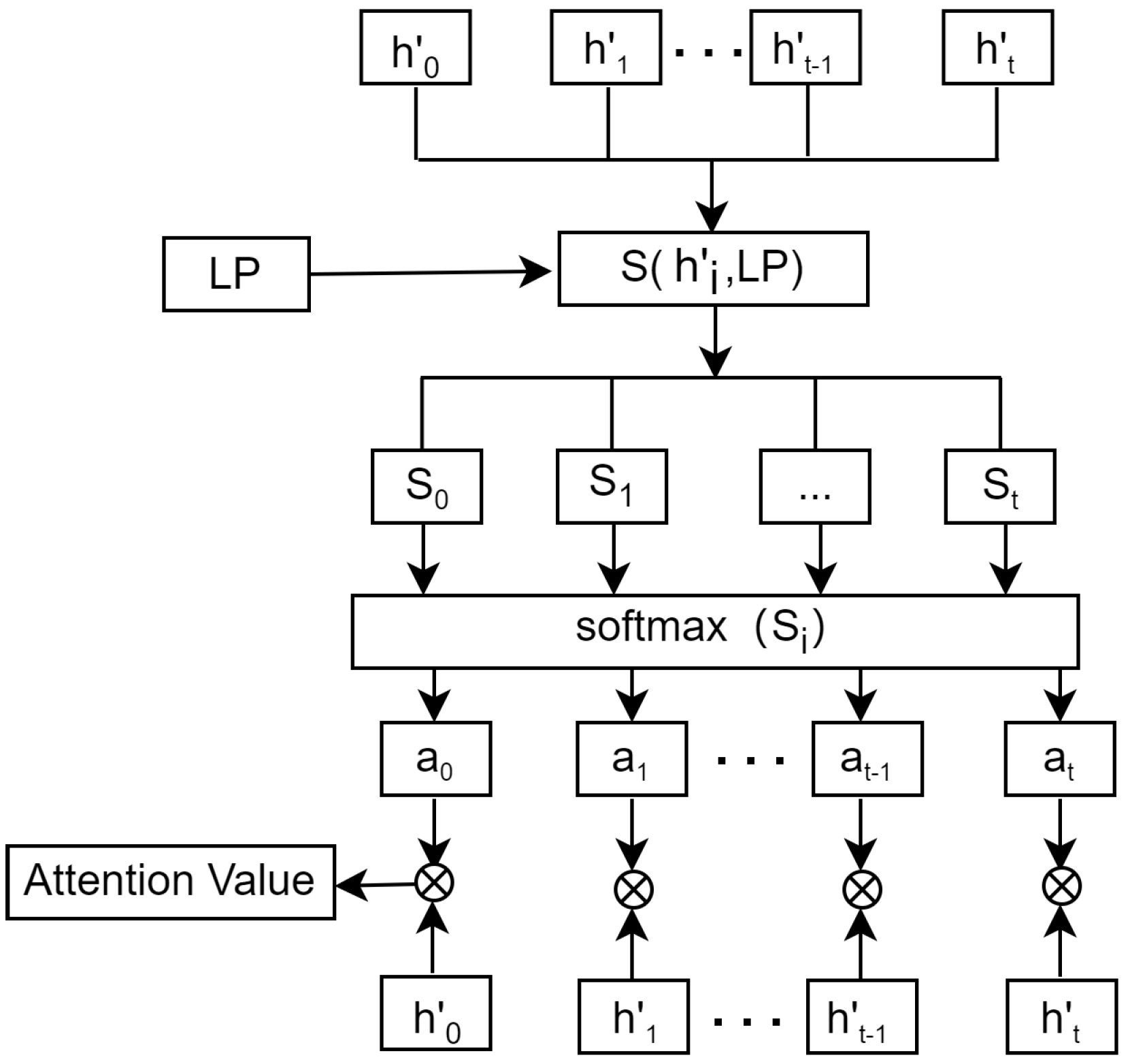
As shown in Figure 4, () is an output eigenvector from the TCN network. LP refers to the forecasting vector. The similarity of (t) and LP is calculated using Equation (18). The attention score can be obtained using the softmax() function. The vector added attention is computed by summing the product of and , as illustrated in Equations (19) and (20). The final prediction value is obtained using a fully connected layer.

Figure 4.
Attention mechanism architecture.
3.5. Price Volatility
Price volatility refers to the fluctuation in price returns within a designated timeframe. When volatility is high, investing in a commodity becomes more precarious. Logarithmic returns offer a more accurate description of price performance. The computation for log returns is illustrated in Equation (21).
where represents the rate of return (…n) and n signifies the sample size. Additionally, stands for the variable’s price at the conclusion of the ith time interval. Simultaneously, the standard deviation of the sample is outlined in Equation (22). The volatility is determined using the sliding window method.
where the standard deviation is computed within each window, represents the mean of logarithmic returns within the sliding window, and represents the overall volatility as shown in Equation (23).
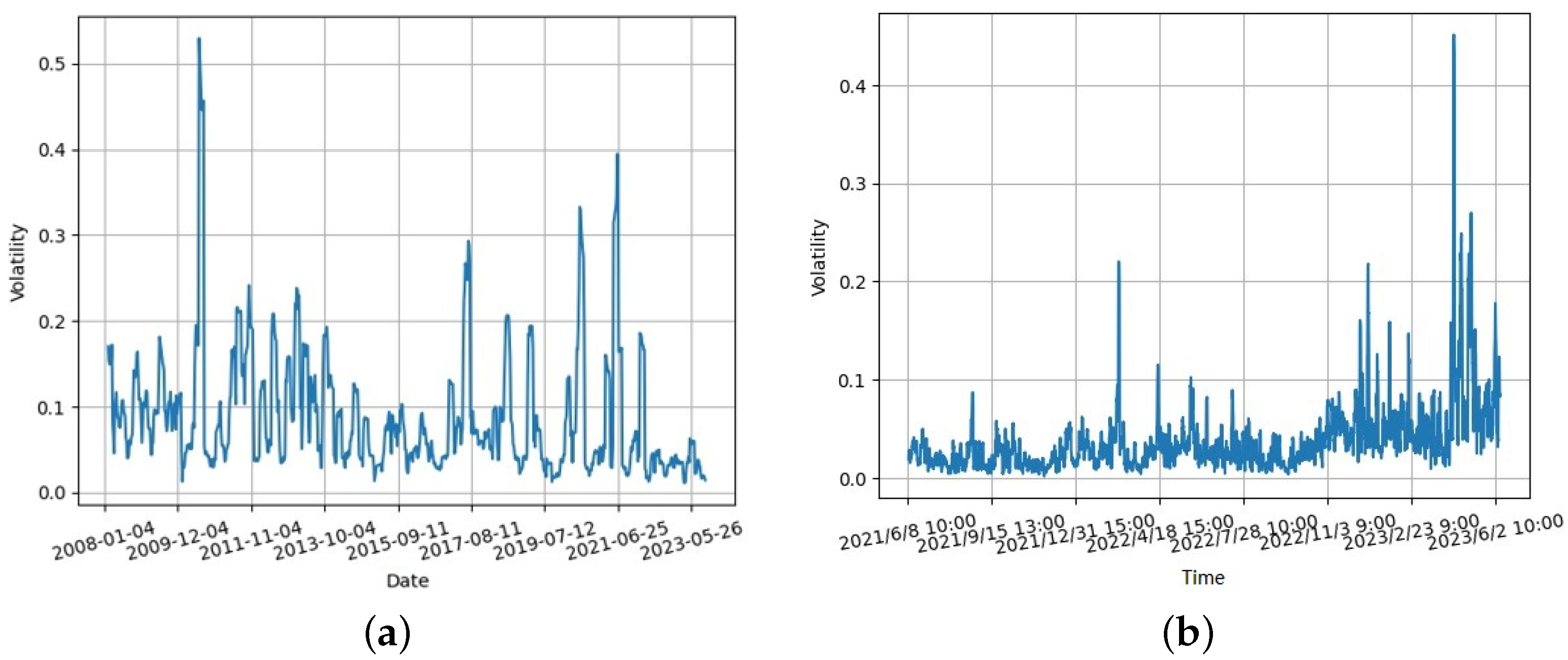
where T is the minimum period required to specify the minimum number of non-missing values needed in the rolling window. The calculation of volatility involves the use of the rolling window method with a minimum period of 5 and a window size set to 7. The changes in price volatility shown in Figure 5a,b were obtained based on original garlic prices from 2008 to 2023 and from June 2021 to June 2023, respectively.

Figure 5.
Price volatility for garlic: (a) spot transaction; and (b) electronic trading.
3.6. Error Evaluation
The metrics , , and are calculated using Equations (24)–(26):
where , , and indicate the actual value, the predicted value, and the average value, respectively, and n denotes the sample size.
4. Experimental Results
4.1. Actual and Synthetic Values
The used data sets were mainly sourced from domestic exchanges of international bulk commodities (https://www.pibce.com/, accessed on 24 September 2024), including 15 features such as trade funds, trade quantity, and trade price. The online electronic trading data for garlic, ginger, and chili span two years, with 3524, 3584, and 2152 records from 9 June 2021 to 7 June 2023, respectively.
Each data set comprises seven points, selected each day for two years. Differencing and normalization were applied in the pre-processing stage, and each data set was increased to 24 times the size of the original data set through data augmentation. The resulting data sets of garlic, ginger, and chili prices were utilized to forecast data across various scales, such as at the hourly or daily level.
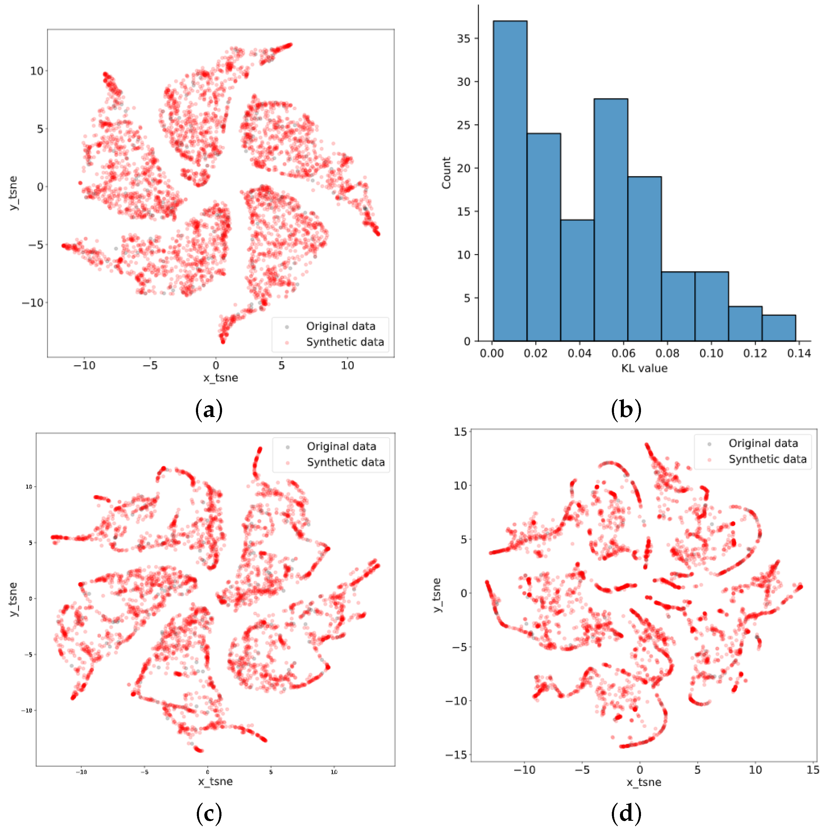
During the training of TimeGAN, the sequence length was set to 24, the learning rate was set to , and 5000 epochs were set. After dimensionality reduction using t-SNE, the original data points fit well with the synthetic data points and had substantial similarity. The results of t-SNE for garlic, ginger, and chili data are depicted in Figure 6. Meanwhile, the KL divergence was calculated for the purpose of quantitative analysis, comparing original data with synthetic data based on 24 records for each group within the first 3504 records, as shown in Figure 6b.

Figure 6.
Results of t-SNE: (a) garlic; (b) KL of garlic; (c) ginger; and (d) chili.
4.2. Feature Importance
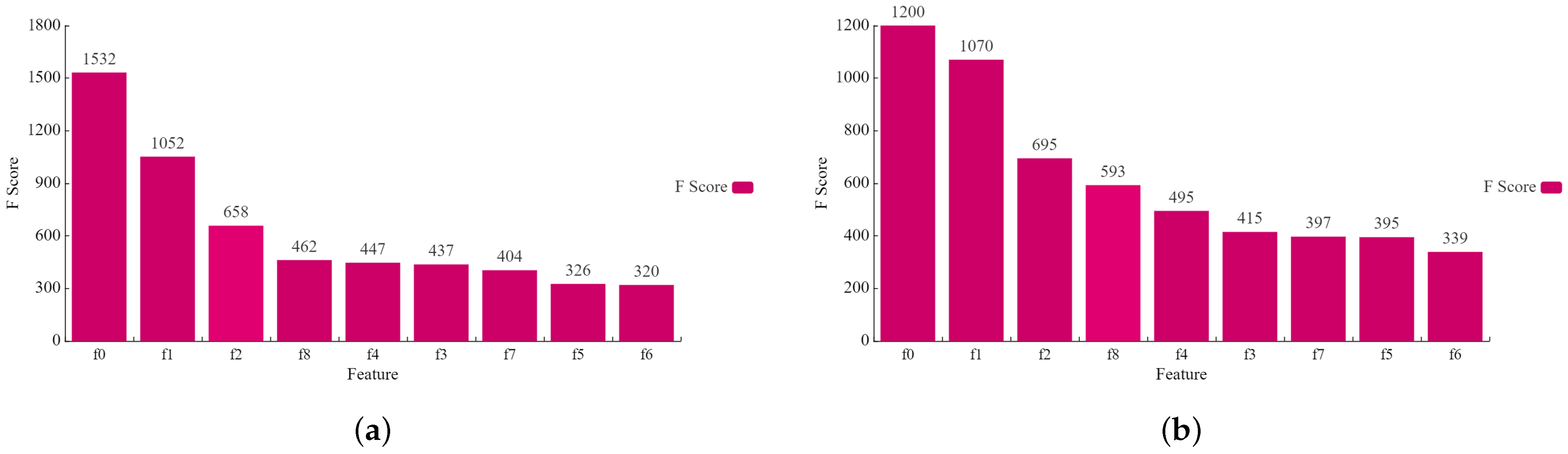
Feature extraction was performed using the XGBoost algorithm, with important features chosen based on F-scores. These important features were then used as input for the TCN-Attention model. Figure 7 shows the feature scores of the synthetic data for garlic and chili data.

Figure 7.
Feature importance results: (a) garlic; and (b) chili.
4.3. Price Forecasting
The experiment leveraged electronic transaction data to assess the effectiveness of the proposed model. The garlic, ginger, and chili data sets were utilized for forecasting at various intervals, including hourly and daily scales. Each data set comprised 10 features relevant to prediction, structured in hourly units, with seven data points chosen per day. Daily data were derived from the averaging of hourly data points for each day.
4.3.1. Data Training and Prediction at the Hourly Level
For the hourly data, the original data were utilized to generate the data set, with a sliding window size of 24 and a stride of 1, via data augmentation. During pre-processing, standardization and normalization were carried out. The training data were enhanced by generating additional data, with the training set being composed of generated data and a portion of the original data set. Additionally, a similarity comparison was conducted using t-SNE.
The experimental results of forecasting were evaluated according to the MAE, RMSE, MAPE, and values. Multi-scale prediction for the three commodities was performed based on the hourly or daily data. The parameter settings were as follows: kernel size of 3, 30 and 100 iterations, learning rate of 0.001, time window set to 5, and Adam optimizer.
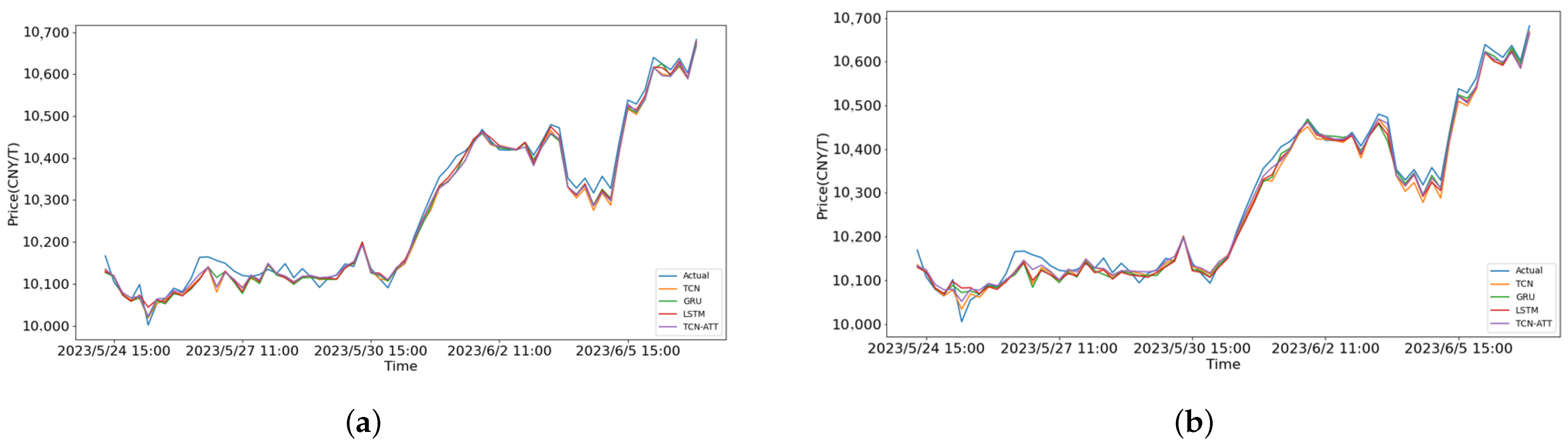
From Table 2, we can see that the TCN-attention and TCN models took less time than GRU or LSTM, and TCN-attention generally performed better overall. Meanwhile, the outcomes of training data for garlic, ginger, and chili with 30 and 100 iterations are presented. Traditional methods such as SVM, RF, and ARIMAX, along with univariate analysis, were added at an hourly level for chili, as shown in Table 3. It can be seen that the accuracy for different species is lower than that of the proposed method. In Table 4, the forecasting results for the next 5 and 10 h on the test sets are presented. Compared with GRU and LSTM, TCN-Attention had better accuracy, slightly outperforming TCN. The comparison of various forecasting methods, including TCN, GRU, LSTM, and TCN-Attention, is illustrated in Figure 8. The figures depict a performance comparison between 30 epochs and 100 epochs for forecasting within the next 10 days. Additionally, the proposed model tended to converge after 30 training iterations.
Table 2.
Training evaluation.
Table 3.
Training evaluation of ML methods.
Table 4.
Forecasting at the hourly level.
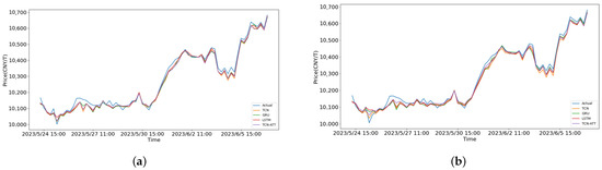
Figure 8.
The forecasting results for garlic in the next 10 days: (a) 30 epochs; and (b) 100 epochs.
4.3.2. Price Forecasting at the Daily Level
The results of price prediction for the next 5 and 10 days at a daily level are compared in Table 5 with 30 iterations. The accuracy of the 5-day forecast is better than that of the 10-day forecast. For garlic, TCN achieved the lowest MAE and RMSE in price forecasting. For chili, TCN-Attention demonstrated better predictive performance in terms of MAE, RMSE, and MAPE; however, it is worth noting that the forecasting accuracy at the daily level was lower than that at the hourly level, and the attention mechanism was not always effective.
Table 5.
Forecasting at the daily level.
4.3.3. Ablation Study
In the ablation experiments, XGBoost+TCN-Att and Timegan+TCN-Att are univariate price prediction, while XGBoost+TCN-Att and the proposed method are multi-variate forecasting as shown in Table 6. The R² of the proposed method is higher than that of several other univariate and multivariate prediction methods. Although the accuracy of proposed method is similar to that without TimeGAN, the method presented may avoid overfitting and better reflect the relationships among time-series, ensuring stable forecasting performance.
Table 6.
Ablation experiments.
5. Discussion
During the development of our research, it was observed that seasonal commodities typically have a small sample size and long data collection intervals, prompting us to propose a strategy to address this issue. TimeGAN has been widely used in engineering fields, but is less common in the domain of bulk commodities. Our experiments revealed that the accuracy of forecasts for periods extending beyond 10 days or 10 h is relatively low. However, predictions for 5 days and 5 h tended to converge after approximately 30 iterations, demonstrating practical value. During the experiments, a low-cost GPU was used, and the model’s stability was validated through the ablation experiments detailed in Section 4.3.3. As the model was applied to real-time data, only its usability was verified in this study. In future research, more influencing factors—such as weather, exchange rates, and regional differences—should be incorporated for further validation. Based on the experimental results, we discuss various issues below.
On one hand, the error evaluation indicated that the proposed method may provide improved accuracy when compared to various existing methods. It performed better than machine learning methods such as SVR or RF. Furthermore, TCN-attention and TCN cost less time than GRU and LSTM, but the running time is also related to parameter settings. The traditional Transformer model presented a negative and, so, does not accurately capture the relationships between sequences. The accuracy ofTimesNet was similar to that of the proposed method, and its accuracy is closely related to its parameter adjustment. For the TimesNet algorithm, the values for the next 5 h were 0.981, 0.874, and 0.328, while those for the next 5 days were 0.950, 0.793, and 0.806. Considering its deployment cost and parameter volume, it was not adopted in the proposed application. On the other hand, the proposed model converged in accuracy at 30 iterations, and excessive iterations in training may lead to overfitting or decreased accuracy. Additionally, the limited range of volatility values has an impact on the accuracy of volatility prediction. In future work, the generalization ability of the model should be further improved.
6. Conclusions
This study proposed a cost-effective method with low run-time for predictive analysis using deep learning models on small sample data. Furthermore, the generalization ability of the model in a practical application considering bulk agricultural commodities was assessed based on previous research outcomes from different perspectives.
A forecasting method combining TimeGAN with TCN-attention was presented for small sample data of agricultural commodities. The proposed approach tackles the issues of overfitting and gradient disappearance, enabling prediction on small sample data. TimeGAN is utilized to augment the obtained data, with similarity evaluation of the synthetic data conducted using t-SNE. Meanwhile, XGBoost is exploited to extract important features. Subsequently, price forecasting is performed with TCN-attention. The results of experiments comparing the proposed model with the TCN, GRU, and LSTM models demonstrated that the proposed method can increase the data volume for small samples, mitigate overfitting, and enhance the prediction accuracy.
When dealing with small-sample data, the proposed method improves the model’s training performance. However, for different varieties, accuracy improvement requires parameter adjustment, and it is essential to further enhance the generalization ability of the model with respect to different varieties. In practical applications, method selection must also take deployment costs into account, as newer methods with deep network layers often pose higher demands regarding the hardware configuration. Additionally, attention should be paid to the interpretability of prediction models in order to improve the reliability of price forecasting in real-world scenarios. The presented method is not limited to agricultural products. Additionally, the method combining XGBoost with TCN-Attention was utilized in our previous publications on power load forecasting, demonstrating the method’s generalization performance. However, the proposed method faces limitations in terms of volatility forecasting, due to the minimal fluctuations in the normalized data. Optimizing the data augmentation algorithm is crucial for enhancing the effectiveness of model training in improving its volatility prediction performance, and further research is needed to tackle the issue of sparse data forecasting.
Author Contributions
Methodology, T.Y. and Y.L.; validation, T.Y. and Y.L.; data curation, T.Y. and Y.L.; writing—original draft preparation, Y.L.; writing—review and editing, Y.L.; visualization, T.Y.; project administration, Y.L.; funding acquisition, Y.L. All authors have read and agreed to the published version of the manuscript.
Funding
The work was supported in part by the Science and Technology Planning Project of Beijing Municipal Education Commission (No. KM202011232022).
Institutional Review Board Statement
Not applicable.
Informed Consent Statement
Not applicable.
Data Availability Statement
The original contributions presented in the study are included in the article, further inquiries can be directed to the corresponding author.
Acknowledgments
The authors wish to thank H.L. Jiang for valuable advice and S.J. Wang for assistance with the experiments.
Conflicts of Interest
The authors declare no conflicts of interest.
References
- Hu, Y. Research on the Characteristics, Reasons and Countermeasures of Current Bulk Commodity Price Rising. Price Theory Pract. 2021, 61–64. [Google Scholar] [CrossRef]
- Liu, X.; Wang, S. Research on mean spillover effect of Sino US soybean futures. Price Theory Pract. 2018, 86–89+102. [Google Scholar] [CrossRef]
- Ge, Y.; Xu, X.; Yang, S.; Zhou, Q.; Shen, F. Survey on Sequence Data Augmentation. J. Front. Comput. Sci. Technol. 2021, 15, 1207–1219. [Google Scholar]
- Zhao, K.; Jin, X.; Wang, Y. Survey on Few-shot Learning. J. Softw. 2021, 32, 349–369. [Google Scholar]
- Pan, Y.; Jing, Y.; Wu, T.; Kong, X. Knowledge-based data augmentation of small samples for oil condition prediction. Reliab. Eng. Syst. Saf. 2022, 217, 108114. [Google Scholar] [CrossRef]
- Li, D.C.; Lin, L.S.; Chen, C.C.; Yu, W.H. Using virtual samples to improve learning performance for small datasets with multimodal distributions. Soft Comput. 2019, 23, 11883–11900. [Google Scholar] [CrossRef]
- Wang, Y.X.; Girshick, R.; Hebert, M.; Hariharan, B. Low-shot learning from imaginary data. In Proceedings of the IEEE Conference on Computer Vision and Pattern Recognition, Salt Lake City, UT, USA, 18–23 June 2018; pp. 7278–7286. [Google Scholar]
- Ramponi, G.; Protopapas, P.; Brambilla, M.; Janssen, R. T-cgan: Conditional generative adversarial network for data augmentation in noisy time series with irregular sampling. arXiv 2018, arXiv:1811.08295. [Google Scholar]
- Shi, G. The Impact of High-Frequency Trading on Market Risk in China’s Stock Index Futures Market and Risk Warning Research. Ph.D. Thesis, Shanghai University of Finance and Economics, Shanghai, China, 2020. [Google Scholar]
- Engle, R.F. Autoregressive conditional heteroscedasticity with estimates of the variance of United Kingdom inflation. Econom. J. Econom. Soc. 1982, 50, 987–1007. [Google Scholar] [CrossRef]
- Bollerslev, T. Generalized autoregressive conditional heteroskedasticity. J. Econom. 1986, 31, 307–327. [Google Scholar] [CrossRef]
- Taylor, S.J. Modelling Financial Time Series; World Scientific: Singapore, 2008. [Google Scholar]
- Andersen, T.G.; Bollerslev, T. Answering the Skeptics: Yes, Standard Volatility Models Do Provide Accurate Forecasts. Int. Econ. Rev. 1998, 39, 885–905. [Google Scholar] [CrossRef]
- Jabeur, S.B.; Mefteh-Wali, S.; Viviani, J.L. Forecasting gold price with the XGBoost algorithm and SHAP interaction values. Ann. Oper. Res. 2021, 334, 679–699. [Google Scholar] [CrossRef]
- Valente, J.M.; Maldonado, S. SVR-FFS: A novel forward feature selection approach for high-frequency time series forecasting using support vector regression. Expert Syst. Appl. 2020, 160, 113729. [Google Scholar] [CrossRef]
- Sun, S.; Wei, Y.; Wang, S. Exchange Rates Forecasting with Decomposition-clustering-ensemble Learning Approach. Syst. Eng. Theory Pract. 2022, 42, 664–677. [Google Scholar]
- Wang, X.; Wang, Y.; Weng, B.; Vinel, A. Stock2Vec: A hybrid deep learning framework for stock market prediction with representation learning and temporal convolutional network. arXiv 2020, arXiv:2010.01197. [Google Scholar]
- Suhui, L. Stock Price Movement Prediction Based on Multi-sources and Heterogeneous Data. Ph.D. Thesis, University of Science and Technology Beijing, Beijing, China, 2021. [Google Scholar]
- van den Oord, A.; Dieleman, S.; Zen, H.; Simonyan, K.; Vinyals, O.; Graves, A.; Kalchbrenner, N.; Senior, A.W.; Kavukcuoglu, K. WaveNet: A Generative Model for Raw Audio. arXiv 2016, arXiv:1609.03499. [Google Scholar]
- Bai, S.; Kolter, J.Z.; Koltun, V. An Empirical Evaluation of Generic Convolutional and Recurrent Networks for Sequence Modeling. arXiv 2018, arXiv:1803.01271. [Google Scholar]
- Cao, D.; Wang, Y.; Duan, J.; Zhang, C.; Zhu, X.; Huang, C.; Tong, Y.; Xu, B.; Bai, J.; Tong, J.; et al. Spectral Temporal Graph Neural Network for Multivariate Time-series Forecasting. arXiv 2020, arXiv:2103.07719. [Google Scholar]
- Dai, W.; An, Y.; Long, W. Price change prediction of Ultra high frequency financial data based on temporal convolutional network. In Proceedings of the International Conference on Information Technology and Quantitative Management, Chengdu, China, 9–11 July 2021. [Google Scholar]
- Cheng, D.; Yang, F.; Xiang, S.; Liu, J. Financial time series forecasting with multi-modality graph neural network. Pattern Recognit. J. Pattern Recognit. Soc. 2022, 121, 108218. [Google Scholar] [CrossRef]
- Xu, H.; Huang, Y.; Duan, Z.; Wang, X.; Feng, J.; Song, P. Multivariate Time Series Forecasting with Transfer Entropy Graph. Tsinghua Sci. Technol. 2020, 28, 141–149. [Google Scholar]
- Lim, B.; Zohren, S. Time-series forecasting with deep learning: A survey. Philos. Trans. R. Soc. A 2020, 379, 20200209. [Google Scholar] [CrossRef]
- Wen, Q.; Zhou, T.; Zhang, C.; Chen, W.; Ma, Z.; Yan, J.; Sun, L. Transformers in time series: A survey. arXiv 2022, arXiv:2202.07125. [Google Scholar]
- Zhou, H.; Zhang, S.; Peng, J.; Zhang, S.; Li, J.; Xiong, H.; Zhang, W. Informer: Beyond Efficient Transformer for Long Sequence Time-Series Forecasting. In Proceedings of the AAAI Conference on Artificial Intelligence, New York, NY, USA, 7–12 February 2020. [Google Scholar]
- Wu, H.; Xu, J.; Wang, J.; Long, M. Autoformer: Decomposition Transformers with Auto-Correlation for Long-Term Series Forecasting. In Proceedings of the Neural Information Processing Systems, Online, 6–14 December 2021. [Google Scholar]
- Wu, H.; Hu, T.; Liu, Y.; Zhou, H.; Wang, J.; Long, M. TimesNet: Temporal 2D-Variation Modeling for General Time Series Analysis. arXiv 2022, arXiv:2210.02186. [Google Scholar]
- Boursin, N.; Remlinger, C.; Mikael, J.; Hargreaves, C.A. Deep Generators on Commodity Markets Application to Deep Hedging. Risks 2022, 11, 7. [Google Scholar] [CrossRef]
- Liu, Y.; Wang, X.; Wang, S.; Xu, Z. Short-term power load forecasting based on temporal convolutional network. In Proceedings of the 2022 International Conference on Information, Control, and Communication Technologies (ICCT), Astrakhan, Russia, 3–7 October 2022; pp. 1–4. [Google Scholar]
- Wang, S.; Wang, X.; Ting, Y. Feature extraction and price forecasting of Multiple Influencing Factors for Cotton based on XGBoost and TCN-Attention. Comput. Syst. Appl. 2023, 32, 10–21. [Google Scholar]
- Yoon, J.; Jarrett, D.; van der Schaar, M. Time-series Generative Adversarial Networks. In Proceedings of the Neural Information Processing Systems, Vancouver, BC, Canada, 8–14 December 2019. [Google Scholar]
- Van der Maaten, L.; Hinton, G.E. Visualizing Data using t-SNE. J. Mach. Learn. Res. 2008, 9, 2579–2605. [Google Scholar]
- Li, Z.; Liu, Z. Feature selection algorithm based on XGBoost. J. Commun. 2019, 40, 101–108. [Google Scholar]
- Chen, T.; Guestrin, C. XGBoost: A Scalable Tree Boosting System. In Proceedings of the 22nd ACM SIGKDD International Conference on Knowledge Discovery and Data Mining, San Francisco, CA, USA, 13–17 August 2016. [Google Scholar]
Disclaimer/Publisher’s Note: The statements, opinions and data contained in all publications are solely those of the individual author(s) and contributor(s) and not of MDPI and/or the editor(s). MDPI and/or the editor(s) disclaim responsibility for any injury to people or property resulting from any ideas, methods, instructions or products referred to in the content. |
© 2024 by the authors. Licensee MDPI, Basel, Switzerland. This article is an open access article distributed under the terms and conditions of the Creative Commons Attribution (CC BY) license (https://creativecommons.org/licenses/by/4.0/).