Abstract
In wireless communication and radar systems, long-distance signal transmission poses significant challenges that affect overall system performance. In this paper, we propose an innovative bistatic radar cross section (RCS) testing system designed to address these challenges, with a particular focus on its long-distance signal transmission capabilities. This system is capable of accurately measuring the RCS of a target and improving multipath channel modeling accuracy by using precise RCS values. The integrated upper computer software extracts amplitude and phase information from received echo signals, processes these data, and provides detailed outputs including the target’s RCS, one-dimensional image, and two-dimensional image. The experimental results obtained prove that this system can not only achieve effective long-distance signal transmission but also substantially enhance the accuracy of RCS measurements, offering reliable support for multipath channel modeling. However, the conclusions drawn are preliminary and require further experimental validation to fully substantiate this system’s performance. Future work will focus on improving system accuracy, minimizing the impact of environmental noise, and optimizing data-processing methods to enhance the efficiency of wireless communication and radar applications.
1. Introduction
In the last two decades, modern wireless communication system technologies have undergone rapid growth in response to the corresponding demand [1]. The multipath effect, a prevalent phenomenon in wireless communication, occurs when radio signals arrive at the receiving antenna via multiple paths. This effect can arise from factors such as atmospheric ducting, ionospheric reflection, and reflections from surfaces like water bodies, mountains, and buildings. Interference and phase shifts can ensue when the same signal follows different paths to the receiver. Destructive interference resulting from this can cause signal fading, which may render a signal too weak to be reliably received in certain areas. This phenomenon is one of the most important causes of system fading. On the other hand, if multipath effects are utilized effectively, communication efficiency can also be improved. For example, using drones as relay stations can create intentional multipath effects, enabling transmission across obstacles in complex environments [2,3] or ensuring reliable long-distance communication [4,5].
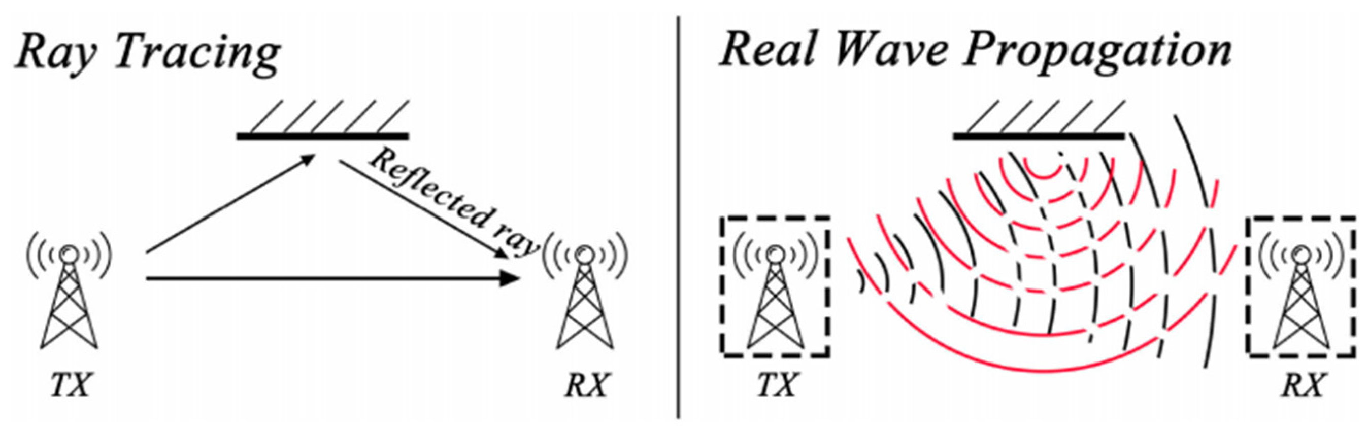
Consequently, a comprehensive understanding of multipath fading channels is crucial for the efficient design of wireless communication systems [6]. In statistical channel models, distribution parameters are typically derived from extensive field measurement data [7], which are used to characterize typical scenarios. Several classical models have been established, such as the 3GPP/ITU 2D/3D channel models and the 3D millimeter-wave channel model [8,9]. However, statistical models frequently fail to precisely capture channel performance at specific locations, leading to the widespread adoption of the ray-tracing method. As shown in Figure 1, the ray-tracing channel model simplifies the wavefront into multiple small ray tubes that propagate along their respective incident directions [10]. It is a deterministic model based on high-frequency electromagnetic simulation technology and uses Maxwell’s equations and appropriate boundary conditions to develop a deterministic model that can ascertain the details of multipath propagation and derive the impulse response of multipath fading for specific environmental conditions [11,12,13].
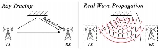
Figure 1.
Comparison between the ray-tracing method and a real situation.
Despite its advantages in providing accurate and detailed modeling of multipath propagation, ray tracing has several inherent drawbacks. One major limitation is its high computational complexity. Additionally, ray-tracing models are highly dependent on detailed and accurate environmental information. Constructing a precise geometric model of the propagation environment, including the shapes, positions, and material properties of all relevant obstacles, can be labor-intensive and time-consuming. Furthermore, while ray tracing can provide detailed insights into a signal’s propagation paths, it does not inherently account for all wave phenomena, such as wave polarization and material anisotropy, which might be relevant in certain scenarios.
Given these challenges, improving the accuracy of multipath channel modeling remains a significant concern in the wireless communication and radar community. Some researchers are attempting to improve the ray-tracing channel model. In [14], Yi Chen et al. explored combining ray-tracing techniques with terahertz communication to enhance multipath channel modeling. Their hybrid approach outperformed conventional models by better capturing the temporal–spatial characteristics of multipath channels and the role of ray tracing in accurate multipath propagation. However, it still faced challenges related to the high computational demands of ray tracing. In [15], Yuanzhe Wang et al. introduced Massive MIMO Communications, emphasizing the need to account for reflection, scattering, and diffraction to obtain more precise results. But they were unable to overcome the challenge of modeling multipath channels in complex environments.
Some other researchers hope to improve the accuracy of multipath channel models by using more novel techniques. Anh Hong Nguyen et al. developed a higher-precision model for specular multipath components (SMCs) using gaussian processes, thereby improving the accuracy of multipath channel modeling for ultra-wideband (UWB) and mm-wave signals [16]. However, in some complex scenarios, Non-Line-of-Sight (NLoS) conditions can severely distort UWB signals, thereby affecting modeling accuracy [17]. To address this issue, Qiu Wang et al. introduced a 1D-ConvLSTM-Attention network (1D-CLANet) enhanced by Squeeze-and-Excitation (SE). This SE-enhanced 1D-CLANet can identify NLoS conditions during modeling. They will use this 1D-CLANet in future research to reduce the modeling errors caused by NLoS conditions [18].
Among the work of researchers, Abdelfattah Fawky et al. creatively demonstrated the importance of incorporating radar cross sections (RCSs) into channel modeling, creating a high-precision 3D deterministic model that provided more accurate predictions of signal behavior in complex environments [19]. This suggests that by accounting for the scattering processes occurring along the signal path in more detail, including the precise RCS values of various scatterers, the overall channel model can be made significantly more accurate. In our paper, we aim to obtain higher-precision RCS values by introducing bistatic testing, and we hope that this high-precision RCS can contribute to developing multipath channel modeling methods that are accurate, have low computational complexity, and are less affected by complex environments.
The RCS of a target represents the effective area perceived by the radar. The formula for defining the RCS is shown in Equation (1) [20]. It is the ratio of the power reflected by a target towards the emission source within a unit solid angle to the plane wave power density incident on the target from a given direction.
In this formula, denotes the RCS, typically measured in or ; represent the distances between the target and the radar’s transmitting and receiving antennas, respectively; is the electric field strength of the scattered wave at the receiving antenna; and is the strength of the incident wave at the target. The RCS is the hypothetical area that intercepts a specific amount of power, which, when scattered uniformly in all directions, produces an echo at the radar station equivalent to that of the actual target. The RCS is the hypothetical area that intercepts a quantity of power such that, when scattered uniformly in all directions, it generates an echo at the radar station equivalent to that of the target. In wireless communication, the radar’s transmitting antenna can be equivalent to the radio wave’s transmitting station, and the radar receiving antenna can be equivalent to the radio wave’s receiving station. Thus, the RCS can characterize the scattering of radio waves by obstacles along the propagation path. The RCS values of some common objects are shown in Table 1 below.

Table 1.
RCS values of common objects [21].
In practical engineering, the RCS definition formula is generally not used. Instead, the radar equation, as shown in Equation (2), is used for RCS measurement [22]. In this formula, represent the radar’s transmitted power and received power, respectively, while correspond to the gains of the transmitting and receiving antennas, respectively. denotes the radar’s operating wavelength.
Traditional RCS testing systems typically use a monostatic radar configuration, where the transmitting and receiving antennas are located at the same radar station. However, with continuous technological advancements, bistatic radar RCS measurements are attracting attention due to their higher accuracy and efficiency [23]. The RCS testing system must ensure coherence between the transmitted and received signals. In monostatic radar systems, where the transmitter and receiver are co-located at the same base station, time and frequency synchronization is readily achievable through the use of a shared clock source, ensuring signal coherence. In bistatic radar systems, where the transmitter and receiver are spatially separated, each must use its own clock. The differences between these clocks make it difficult to coordinate transmission and reception. There are two common methods: One consists of equipping both bases with high-precision atomic clocks. The coherent population trapping (CPT) atomic clock, widely used in synchronization communications, has a frequency stability of approximately , while the highest-precision rubidium atomic clocks can achieve a frequency stability of [24]. However, the production and maintenance costs of high-precision atomic clocks are extremely high. Another method consists of extracting a synchronization signal from one base and transmitting it to another base, thereby achieving synchronization between the two bases. The key to this method is ensuring that the synchronization signal maintains phase stability after long-distance transmission between the two bases.
This article presents a signal transmission system designed for a bistatic RCS testing system to address the issue of time synchronization. As the testing system is an electromagnetic measurement system and the distance between the two radar stations is over 300 m, using wireless electrical signal transmission could interfere with the scattered waves, affecting the test results. On the other hand, using wired electrical signal transmission over such distances would lead to significant attenuation. Therefore, our design adopts an optoelectronic conversion approach. Before transmission, the reference signal is converted into an optical signal, transmitted via optical fiber to the other base station, and then demodulated back into an electrical signal. The optoelectronic conversion system is linear and does not disrupt the coherence of the entire testing system. The linearity of this system is a key indicator in determining whether RCS measurements can be performed. In the following Section 3, the phase stability of the system is specifically tested, and in Section 4, the negative impacts that system nonlinearity may have on the overall RCS measurements are analyzed.
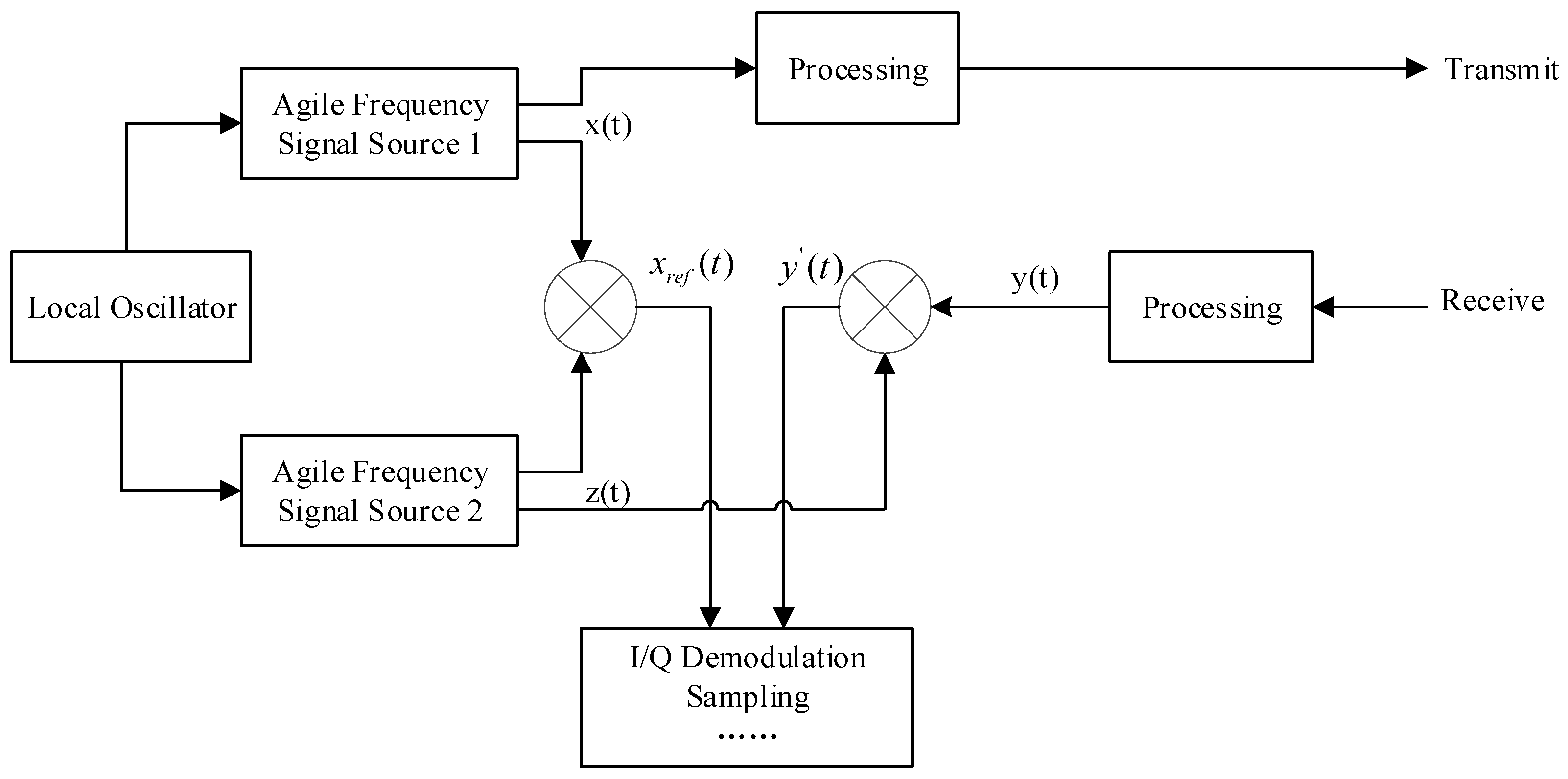
2. System Principle and Simulation
The entire testing system is an inter-pulse frequency-hopping radar, and its operating principle is illustrated in Figure 2. A local oscillator signal provides the time base for two agile frequency signal sources, ensuring time synchronization between them. Agile frequency signal source 1 generates a signal with a frequency , which is split into two paths. One path is used as the transmission signal, which, after modulation, amplitude control, and power amplification, is transmitted towards the target by the antenna. The other path serves as the intermediate frequency (IF) for down-conversion to obtain the signal . The signal generated by agile frequency signal source 2, with a frequency , is also split into two paths. One path is used as the reference local oscillator and mixed with the processed echo signal to obtain signal . The other path serves as the RF input for down-conversion to obtain the signal . Thus, the frequency of signal should be . Finally, the signal this time acts as the IF, and the other signal, , undergoes a series of processes, including sampling, digital phase locking, quadrature digital down-conversion, and baseband signal post-processing. This process allows one to obtain various measurements, such as the target’s RCS, one-dimensional image, and two-dimensional image.

Figure 2.
Schematic diagram of the bistatic testing system.
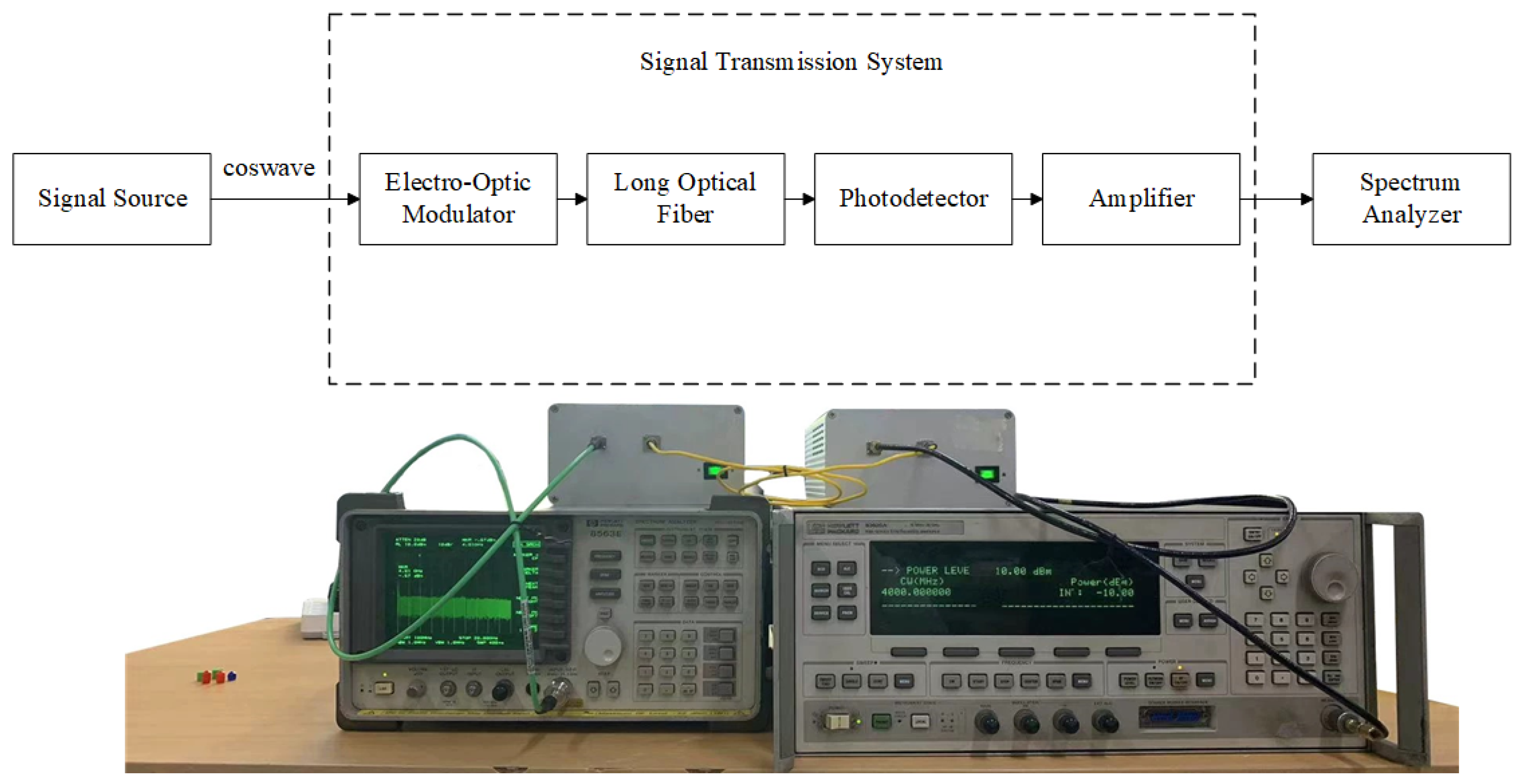
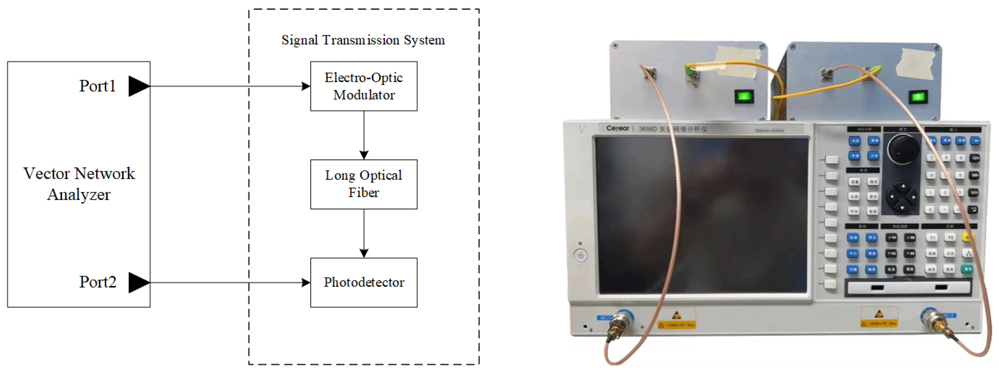
Additionally, the signal transmission system can theoretically be connected at any point in the entire testing system to increase the extent of signal transmission. A schematic diagram of this system is shown in Figure 3.
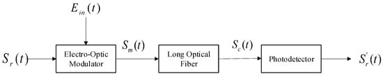
Figure 3.
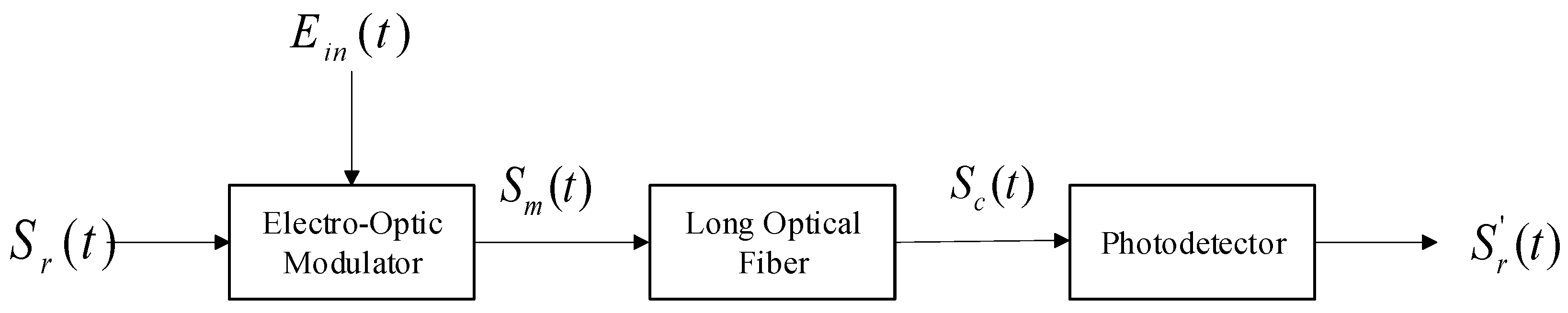
Schematic diagram of the signal transmission system.
The modulated signal, , is input into an electro-optical modulator, where it modulates the optical carrier signal, , generated within the modulator, forming the modulated optical signal, . After long-distance optical fiber transmission, undergoes a phase shift and attenuation, resulting in the optical signal . then enters a photodetector and is converted back into the electrical signal, .
2.1. Selection of an Electro-Optic Modulator
Optical modulators encode an electrical signal onto an optical wave, known as the optical carrier. This encoding can manipulate the amplitude, phase, frequency, polarization, or any combination of these properties of the optical carrier [25]. To meet the demand for long-distance and high-capacity service in modern optical transmission networks, high speed, compactness, and low power have become the mainstream development themes for future electro-optical modulators [26,27]. Among the various electro-optical modulators, the Mach–Zehnder modulator has become one of the most widely used types in recent years due to its advantages: high speed, low cost, and low complexity [28].
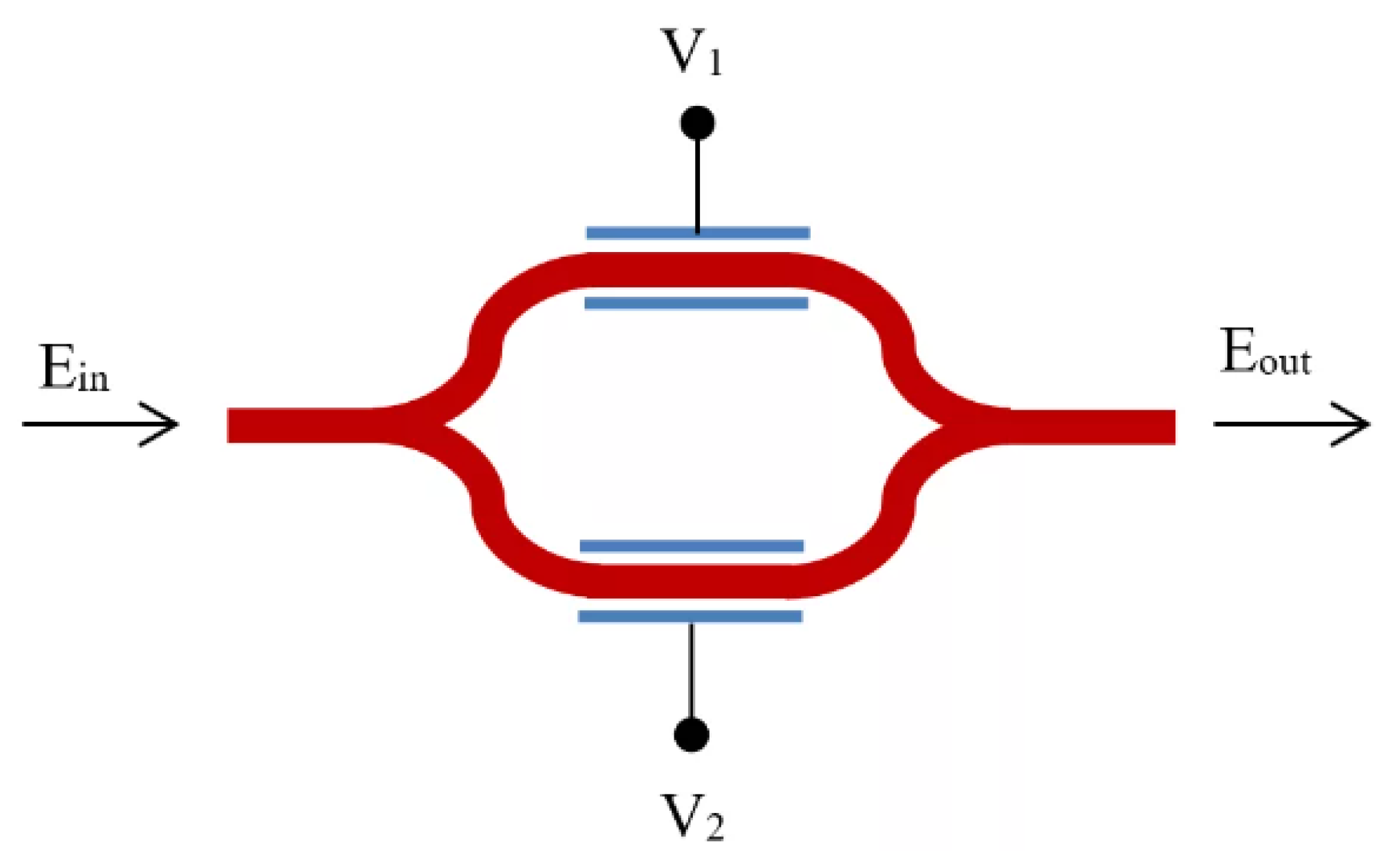
The Mach–Zehnder modulator (MZM) is an interferometric device constructed from a material exhibiting a strong electro-optic effect (such as ). Lithium niobate ()-based MZMs are commonly used for modulation in communication systems with a capacity of up to . However, their application is constrained by high drive voltages, a large physical footprint, and a lack of integrability [29]. In contrast, indium phosphide ()-based MZMs offer higher 3 dB bandwidths and require lower drive voltages [30]. But they are also more expensive than the former. The structure of the MZM is illustrated in Figure 4. The optical input is divided between the upper and lower modulator arms, where phase modulation occurs via two phase shifters driven by the electrical signals . The modulated signals are then recombined to produce the optical output .

Figure 4.
A schematic diagram of the MZM.
The MZM has three operating modes: Maximum Transmission Point (MATP), Quadrature Point (QTP), and Minimum Transmission Point (MITP). By setting an appropriate DC bias voltage, the operating mode of the MZM can be selected. When the bias voltage is set to 0, the MZM is in the MATP mode, and the output optical intensity is at its maximum. In this mode, since the bias voltage is 0, the refractive indices of the upper and lower arms do not change, and the optical signals in both arms are not modulated. When the bias voltage is set to half of the modulator’s half-wave voltage, the MZM is in the QTP mode, and the output optical intensity is half of the maximum optical intensity. The externally applied voltage alters the refractive indices of the upper and lower arms, causing the optical signals in each arm to undergo varying levels of phase modulation. This process induces a phase shift between the optical signals in the two arms, resulting in a coherent superposition within the optical coupler. When the bias voltage is set to the modulator’s half-wave voltage, the MZM is in the MITP mode, and the output optical intensity is 0. In this mode, when the DC bias voltage is equal to the MZM’s half-wave voltage, the optical amplitudes in the upper and lower arms cancel each other out in the optical coupler, resulting in an output optical field of 0.
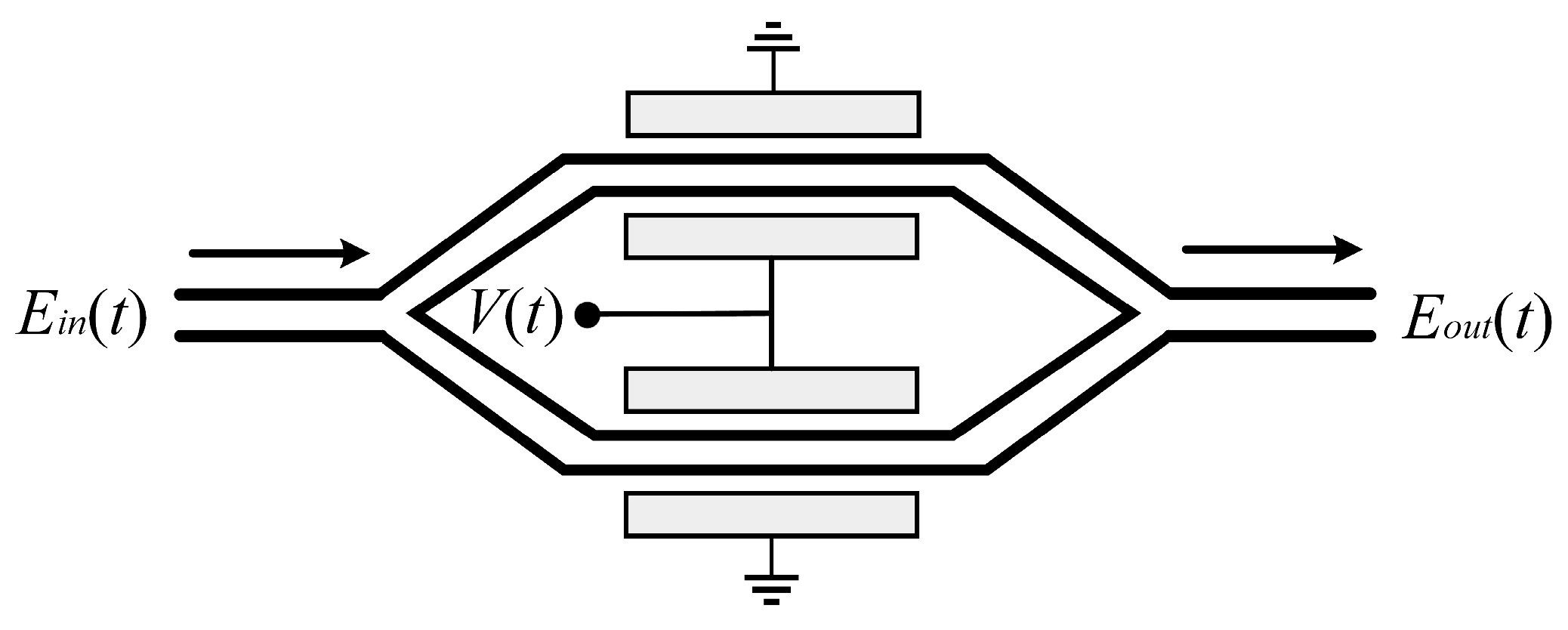
As the MZM is one of the more mature technologies among the various optoelectronic modulation methods, with relatively simple principles and moderate hardware costs, we employed an MZM operating in single-drive push–pull mode, which modulates the signal in terms of amplitude. In the push–pull-mode MZM, there is only one radio frequency (RF) electrode and one direct current (DC) electrode, as depicted in Figure 5. Two RF signals of equal amplitude and opposite phases are applied to the upper and lower arms of the MZM. The MZM operates in the QTP state to avoid the need for carrier and phase recovery [31]. In this state, only the intensity modulation of the input optical signal occurs. The output of the modulator in this operating mode can be represented as follows:
in which represents the optical carrier signal input to the MZM, denotes the insertion loss of the MZM, is the half-wave voltage of the modulator, and represent the amplitude, angular frequency, and initial phase of the modulating signal , respectively. represents the DC bias voltage applied to the upper and lower arms.
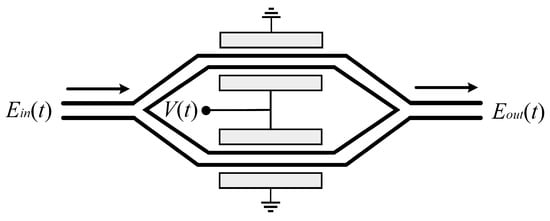
Figure 5.
A schematic diagram of the single-drive push–pull-mode MZM.
2.2. Derivation of the System Formulas
Let us assume the modulating signal in Figure 2 is a standard cosine signal:
is the amplitude of the modulating signal. and represent the angular frequency (the following will be referred to as “frequency”) and initial phase of the modulating signal, respectively. Since the MZM operates in QTP mode, . Therefore, the modulated optical signal obtained after the modulating signal passes through the electro-optic converter can be represented as follows:
In this formula, represents the optical carrier signal:
represents the amplitude of the optical carrier signal, and represent the frequency and phase of the optical carrier signal. denotes the insertion loss of the modulator, and is approximately 6 V in this design. is referred to as the modulation index.
According to the Jacobi–Anger expansion,
By substituting Equation (7) into Equation (5), we obtain the following:
Here, represents the first-kind n-order Bessel function. In the case of small signal modulation, only the DC component and the first-order component are considered. Therefore, the above equation can be written as follows:
The signal undergoes transmission through a single-mode fiber (SMF) with a length of , wherein the transfer function of the SMF is given by the following:
represent the length, propagation constant, and amplitude attenuation coefficient of the SMF, respectively. By performing a Taylor expansion on and using to denote the propagation constant at point and the values of the first and second derivatives, we can obtain the following:
From Equations (9)–(11), we can obtain the expression for the modulated optical signal obtained after it propagates through the SMF with a length of as follows:
Finally, the photocurrent detected by the photodetector is given by the following:
Here, is the responsivity of the photodetector, and represents the power attenuation coefficient of the optical wave during transmission in the fiber. Considering the Taylor series expansion of , the photocurrent can be expressed as follows:
Here, is referred to as the group delay of the carrier, , where , and represent the fiber’s dispersion coefficient, optical wavelength, and the speed of light in a vacuum, respectively. By comparing the input and output of the photoelectric conversion system, it can be observed that, after considering the negative sign in the phase of the first harmonic term of , it can be simplified to . When comparing the phase of the modulating signal , the difference between the two is . The parameter represents the group delay of the entire system, which is solely determined by the system itself and the length of the optical fiber, making a fixed constant.
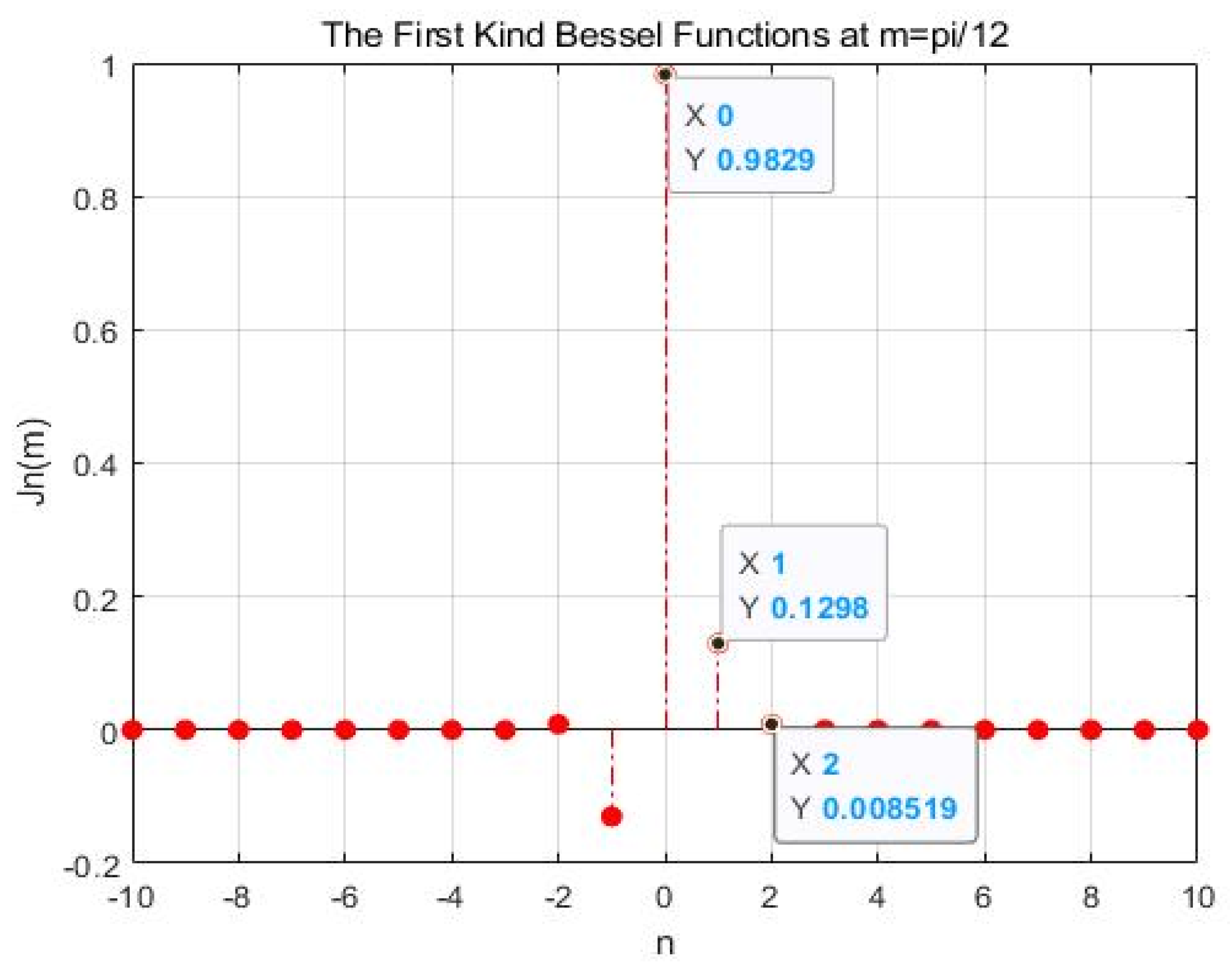
Moreover, as shown by Equation (12), it is evident that the primary factor determining the intensity of the n-th harmonic is the n-th order Bessel function value of the modulation index . As shown in Figure 6, in the case of small-signal modulation, where m is relatively small, for becomes significantly smaller than and ; thus, it can be considered negligible.
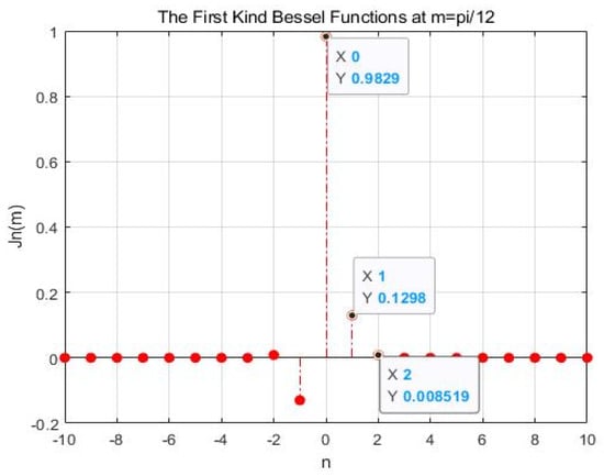
Figure 6.
Bessel function values for .
2.3. System Simulation
In the previous section, we concluded through theoretical derivation that the system fundamentally meets the phase stability requirements. In this stage, we used Matlab 2020a to conduct simulations to gain an intuitive understanding of the waveform and phase variations at each node of the system as well as observe the impact of various component parameters on system gain and waveform.
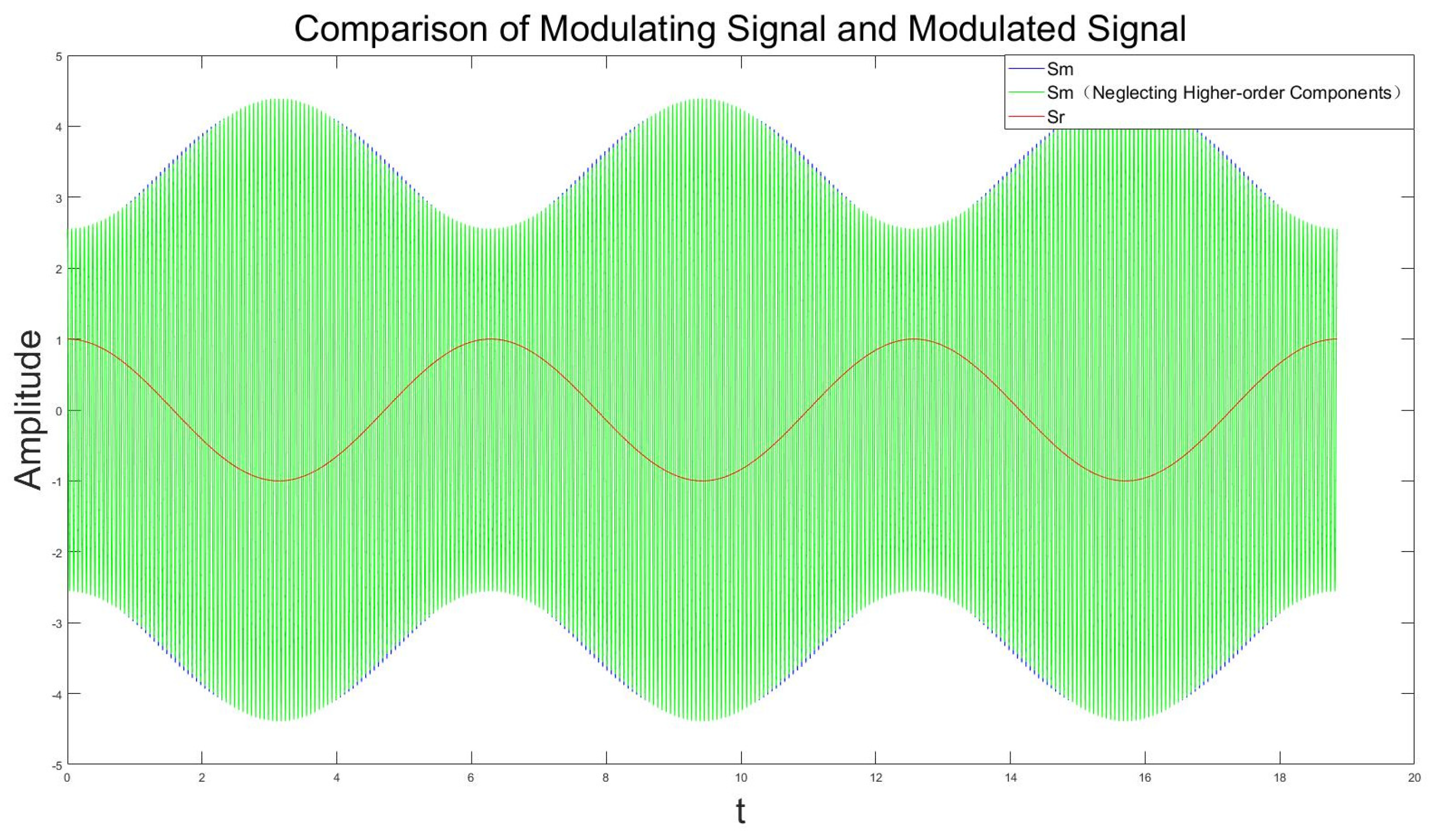
Firstly, we set the simulation parameters for the system. Since the carrier used in the photoelectric conversion is typically a laser with a wavelength of 1550 nm, which corresponds to a frequency of approximately , and the frequency range of the modulated electrical signal is , it follows that in practical applications, . Thus, for the modulating signal, we set the parameters as follows: amplitude , frequency , and initial phase . For the optical carrier signal, we set the amplitude , carrier signal frequency to satisfy the condition for amplitude modulation, and carrier signal initial phase . The half-wave voltage of a MZM is generally between 3 and 10 V. A lower half-wave voltage can enhance the performance of the MZM by increasing the modulation speed, reducing the heat generation, and lowering the drive voltage requirements, thereby improving overall efficiency. However, MZMs with lower half-wave voltages require more complex fabrication processes and incur higher production costs. After comprehensive consideration, the half-wave voltage of the MZM was set to , which is also the voltage used for the actual product. Thus, the modulation index . The insertion loss is . A waveform comparison between the modulated signal and the modulating signal is shown in Figure 7.

Figure 7.
Comparison of the modulating signal and the modulated signal.
In the figure above, the blue and green curves represent the complete modulated signal and the signal with only the DC and first-order components retained, respectively. The red curve represents the modulating signal . It is evident from the figure that the envelopes of the blue and green curves almost entirely match the red curve. Unlike traditional amplitude modulation, the envelope of the modulated signal is no longer perfectly aligned with the phase of the modulated signal but instead undergoes a phase inversion. This is due to the inherent principles of the MZM, as shown in Equation (9). Comparing the blue and green curves shows that they overlap almost completely, with only slight differences around the peaks, confirming the approximation mentioned in Equation (9) that “In the case of small signal modulation, only the DC component and the first-order component are considered”.
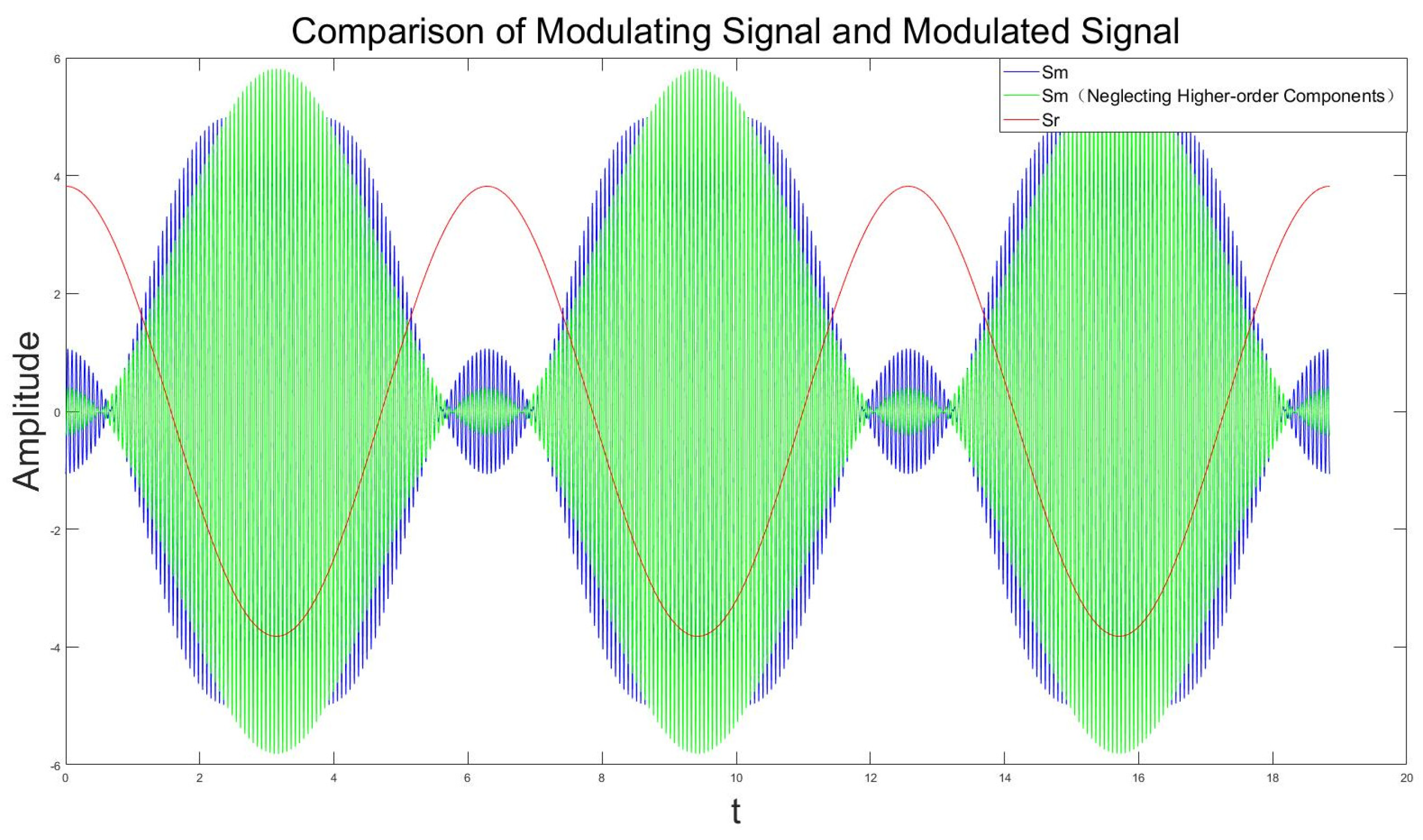
Regarding the case where the modulation index is increased to , a comparison between the true values and the approximate values is shown in Figure 8. At this point, there is a significant difference between the true and approximate values, and neither envelope matches the modulated signal anymore, indicating that the intensity modulation of a single push–pull MZM is only applicable when the modulating signal amplitude is less than the half-wave voltage of the modulator. Therefore, in practical applications, it is essential to control the amplitude of the modulating signal.

Figure 8.
Comparison of the modulating and modulated signals with m = 1.
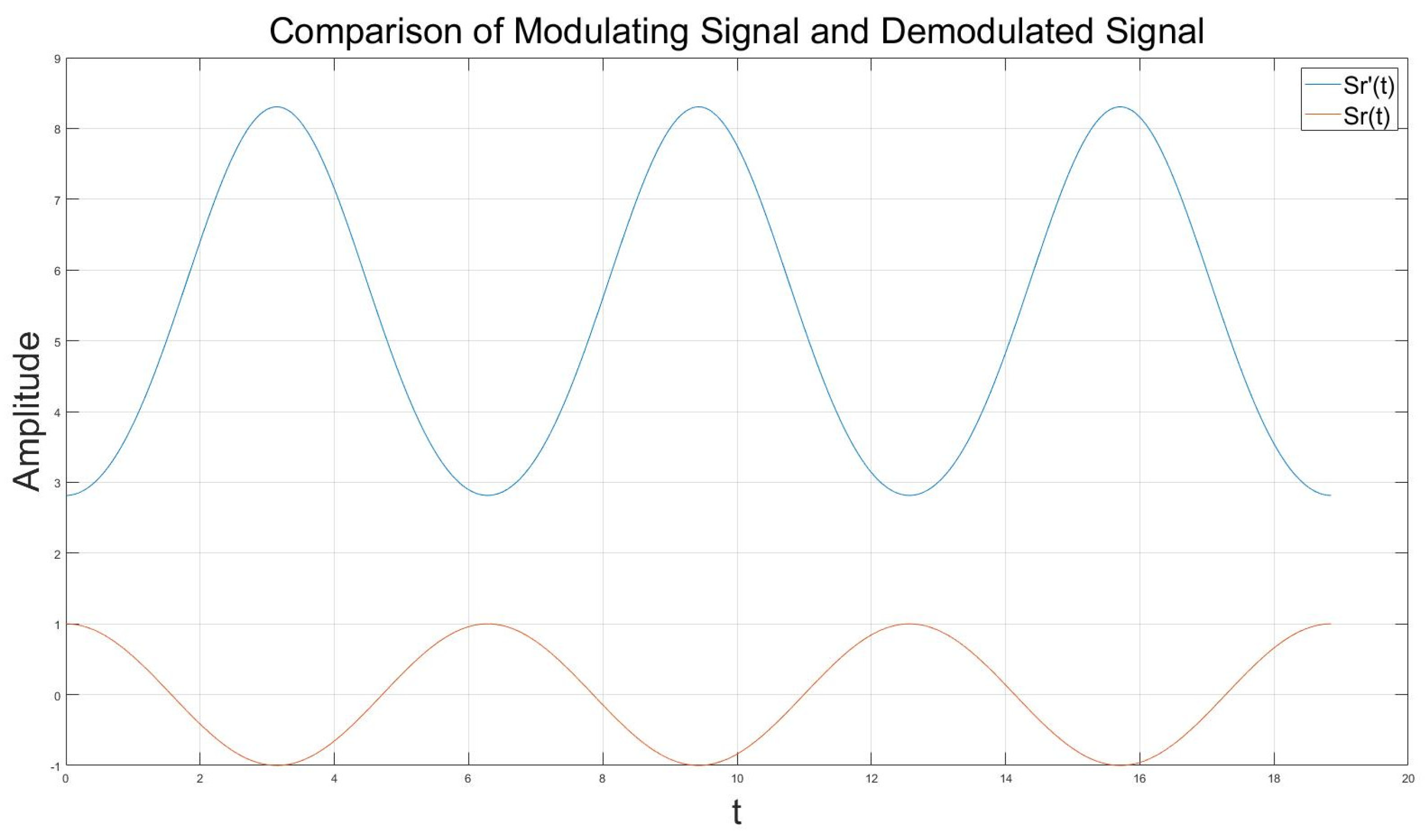
For the optical fiber in the system, the simulation parameters were set as follows: the attenuation coefficient of the fiber , the refractive index , the operating wavelength , and the dispersion coefficient . The length was set to , and a rough calculation revealed that the group delay is . For the photodetector, the responsivity is a positive number that is always less than 1. For convenience in calculations, it was set to . A comparison between the system’s output signal and input signal is shown in Figure 9:
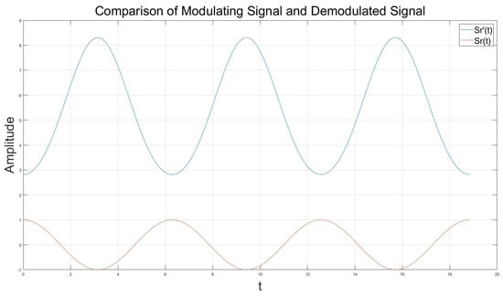
Figure 9.
Comparison of modulating signal and demodulated signal.
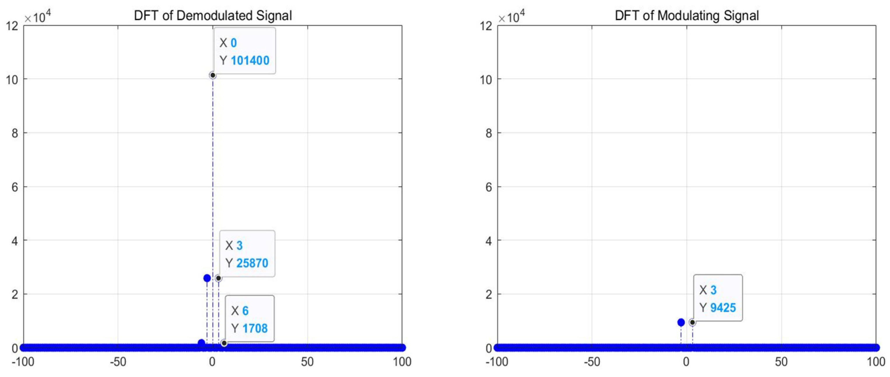
In the figure, it can be observed that the demodulated signal has an added DC component and a higher amplitude than the modulating signal, while the frequency remains almost identical to the input signal. Due to the group delay being only 2420 ns, the phase difference in caused by the group delay is negligible, resulting in a phase difference of between the two signals. Performing a discrete Fourier transform with 18,850 points on the demodulated signal yields the results shown in Figure 10.

Figure 10.
DFT of the demodulated and modulating signals.
Upon comparing the DFT results of the demodulated and modulating signals, it becomes evident that the proportion of the second harmonic component in the demodulated signal is much smaller than that of the first harmonic and the DC component. This also confirms that neglecting the higher-order components of the demodulated signal, as mentioned in Equation (14), is a reasonable approximation.
The simulation results corroborate the theoretical derivations, with both confirming that the system is fundamentally feasible. These findings provided a solid foundation for the subsequent practical measurements. Moving forward, real-world testing will further validate the system’s feasibility and help identify any potential issues that may not have been captured in the theoretical analysis.
3. System Testing
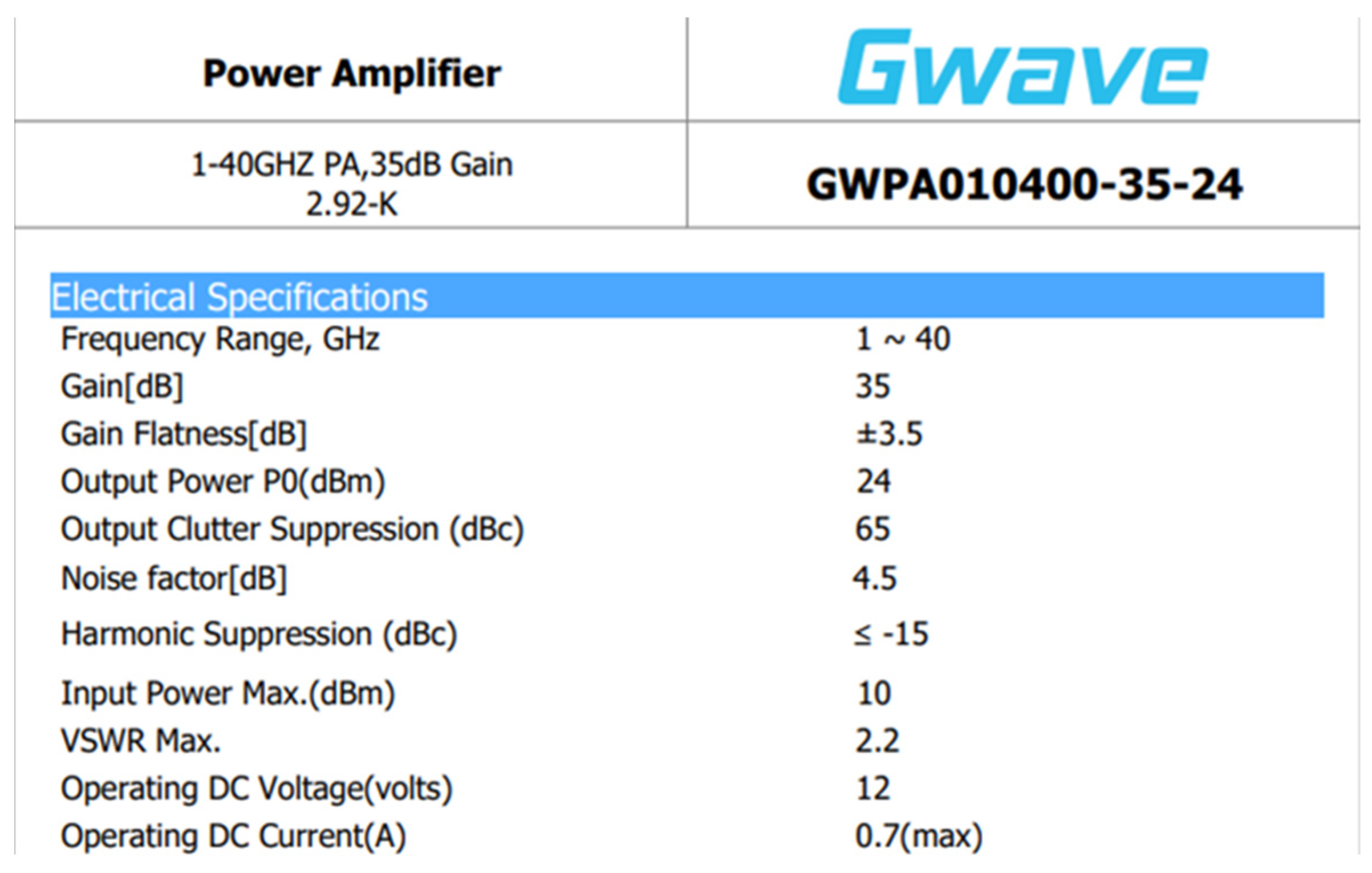
The main goal of these system tests was to validate the performance of the long-distance signal transmission system within the bistatic RCS testing configuration. The tests were designed to obtain information on the gain and phase stability of the signal transmission system to determine whether its integration into the entire testing system would affect the system’s functionality. Additionally, the tests involved the observation of the clutter and higher-order harmonics introduced by the system to assess whether a filtering device was needed. To prevent the amplitude of the photocurrent detected by the photodetector module from being too small, which could affect subsequent signal processing, the system cascades an amplifier model GWPA010400-35-24, made by Beijing Gwave Technology Co., Ltd. (Beijing, China), after the photodetector. The detailed parameters are shown in Figure 11.
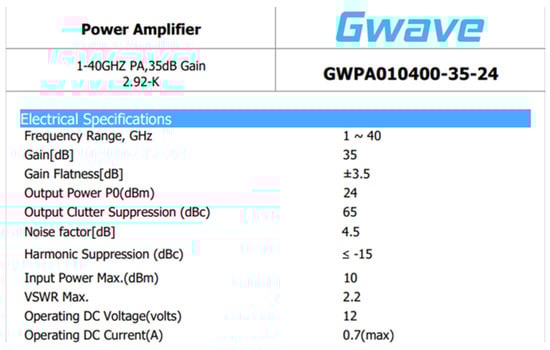
Figure 11.
Parameters of the system-cascaded amplifier.
3.1. Spurious and Higher-Harmonic Testing
When conducting spurious and higher-harmonic testing, a standard cosine signal generated by a signal source is used as the input for the system, and the electrical signal outputted by the system is connected to a spectrum analyzer for analysis. A schematic diagram and the actual setup of the system for testing are depicted in Figure 12.

Figure 12.
Schematic and test setup of the spurious and higher-harmonic test.
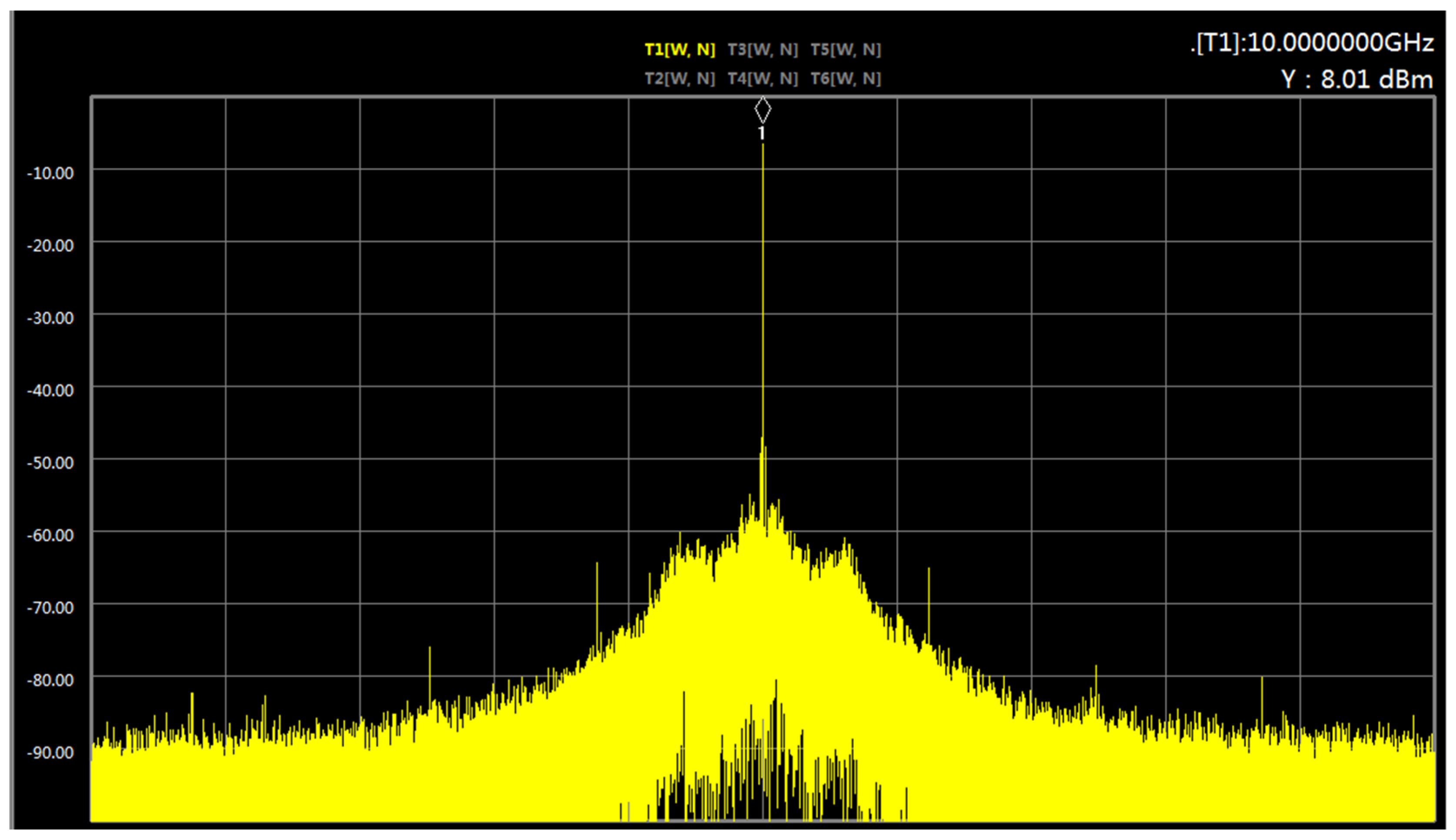
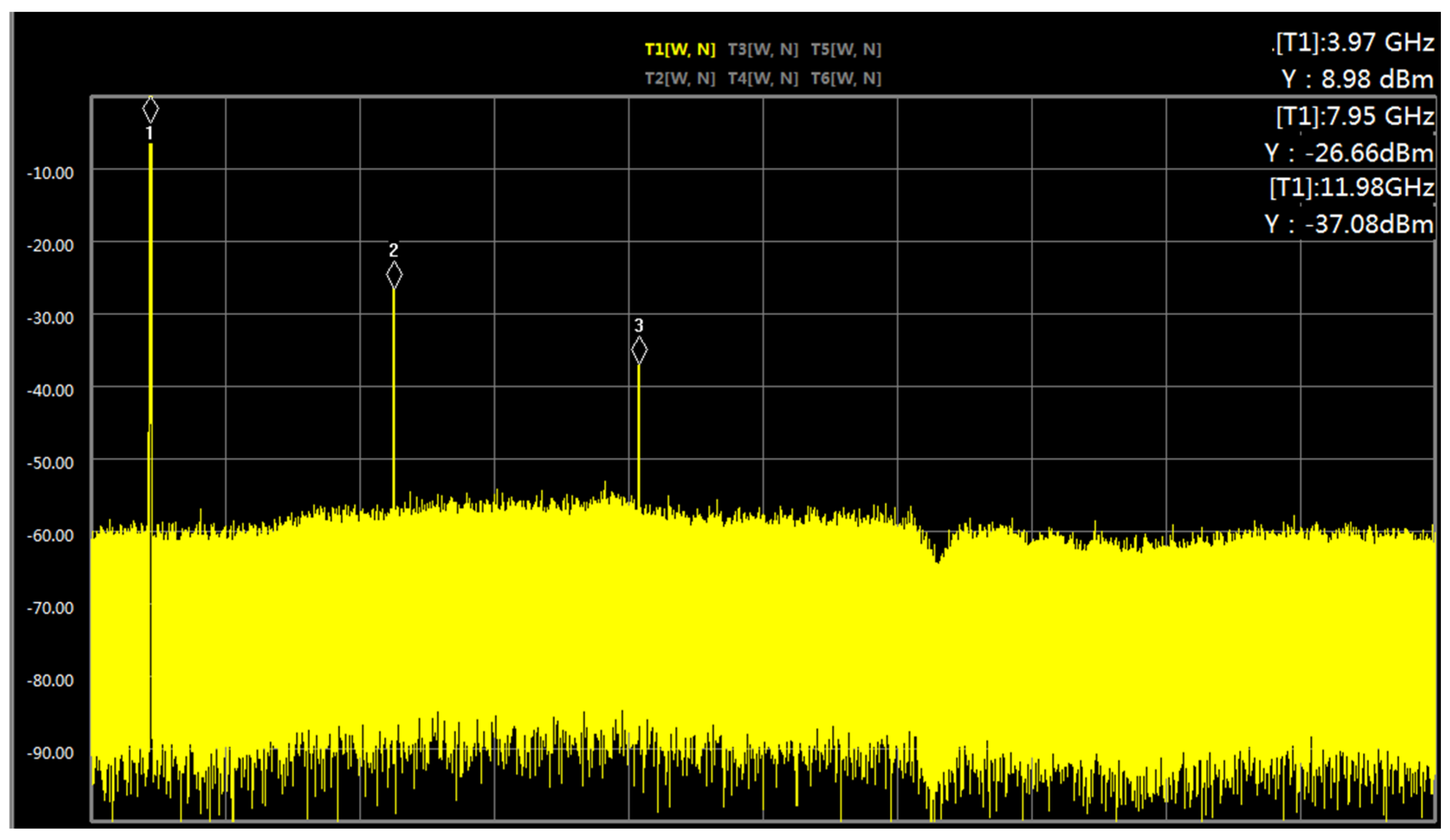
Starting with a representative 10 GHz signal, the spurious conditions of the system were tested. The output frequency of the signal source was set to 10 GHz with a power output of −10 dBm. The resolution bandwidth (RBW) and video bandwidth (VBW) of the spectrum analyzer were set to 10 Hz and 300 Hz, respectively. The spurious conditions around the center frequency were observed, and the results are shown in Figure 13. From the results, it can be gleaned that there was almost no spurious interference from other frequencies near the center frequency. Subsequently, using a 4 GHz signal as a representative, the higher-harmonic conditions of the system were tested. The output frequency of the signal source was set to 4 GHz with a power output of −10 dBm. The frequency sweep range (span) of the spectrum analyzer was set from 1 to 20 GHz to observe the higher-harmonic conditions. The results are shown in Figure 14.

Figure 13.
Spurious test results (diamond shape represents marker).
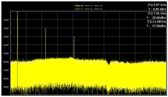
Figure 14.
Higher harmonics at a 4 GHz input (diamond shapes represent markers).
The figure shows that the power of the first harmonic in the output signal is 8.98 dBm, while the power of the second harmonic is only −26.66 dBm, which is 35.64 dB lower than the first harmonic, consistent with the conclusion in Section 2. Additionally, it can be noted that there are third-order harmonics present in the system output; these were introduced by the amplifier cascaded after the photodetector. The power of the third harmonic is 46.06 dB lower than that of the first harmonic, almost negligible, and does not affect the normal operation of the system. The test results for higher harmonics at other frequencies are summarized in Table 2.
Table 2.
Higher harmonics at various frequencies with −10 dBm of input power.
The test results indicate that the signal transmission system does not necessarily require a filtering device. However, if conditions allow for the introduction of a filtering device, such a device can reduce the interference from the existing spurious and higher-order harmonics.
3.2. Dynamic Range Testing
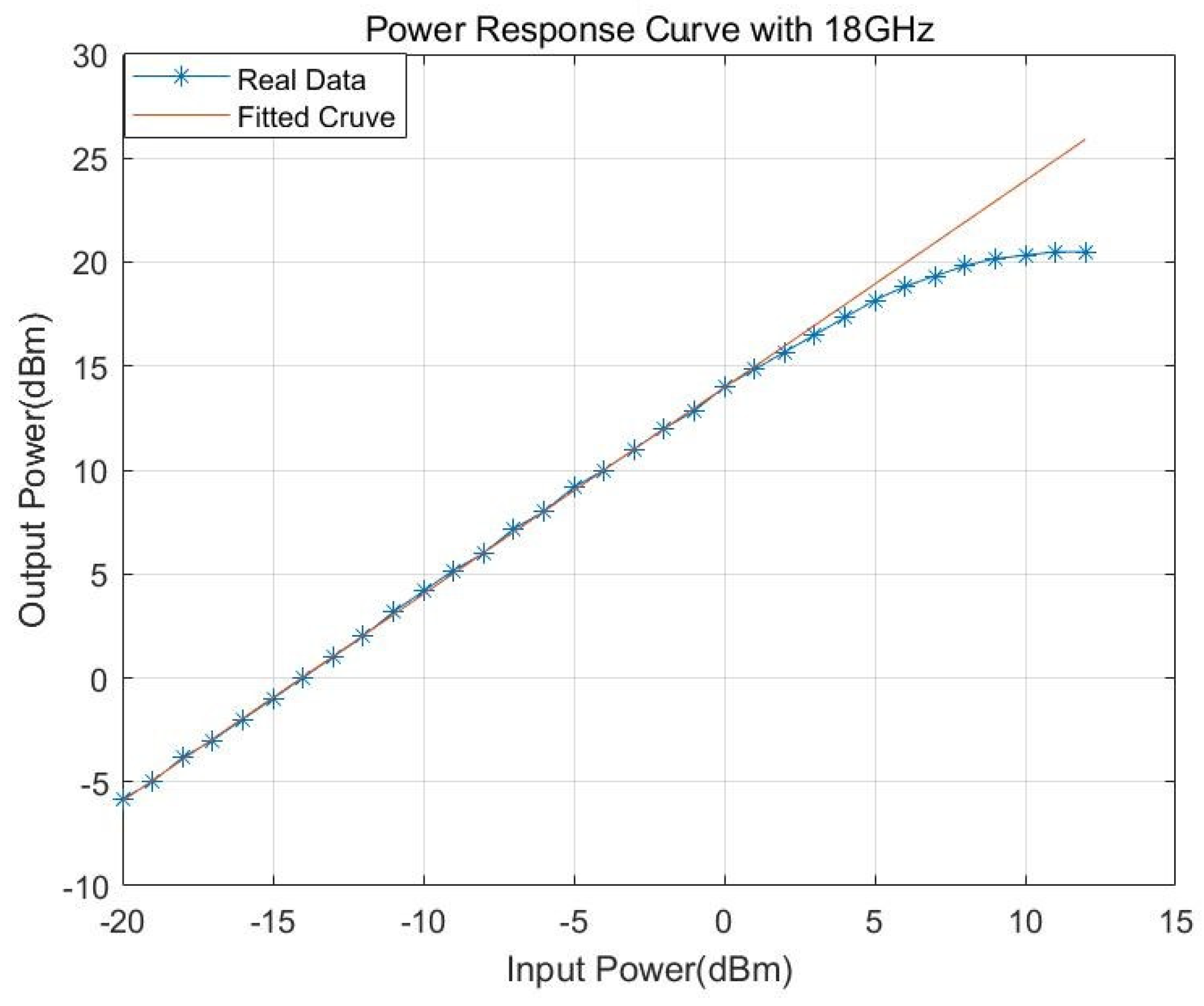
The principle and environment for dynamic range testing are the same as those in Section 3.1. Using an input signal frequency of 18 GHz as an example, the input–output response curve of the system is shown in Figure 15.
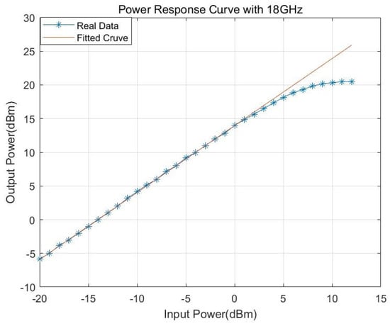
Figure 15.
Power response curve with 18 GHz.
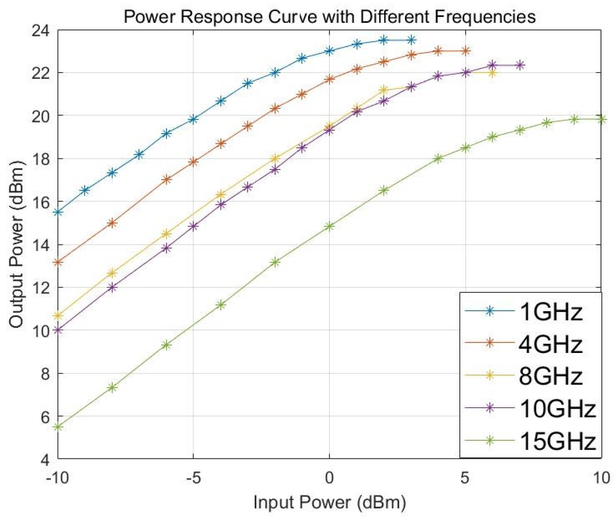
In the figure, the blue curve represents the measured data, while the red curve is the fitted curve for the linear region, with the following fitting equation: . The line loss at 18 GHz is 4.65 dBm, resulting in a calculated linear region gain of 18.66 dBm for the system at 18 GHz. The saturation input power is approximately 10 dBm, and the saturation output power is around 20.5 dBm. Using the same method, the test results at 1 GHz, 4 GHz, 8 GHz, 10 GHz, and 15 GHz are shown in Figure 16.

Figure 16.
Power response curve with different frequencies.
Finally, the system’s gain, saturation input power, and saturation output power are summarized in Table 3.
Table 3.
Dynamic range test results for the system.
3.3. Phase Stability and Group Delay Testing
A principle diagram and the testing environment for system phase stability testing are shown in Figure 17. The system was connected to a vector network analyzer, and the S21 parameter of the network analyzer was used to obtain the group delay and the phase variation of the system over 8 h of continuous operation at different frequencies. The system group delay was determined to be 1503 ns.

Figure 17.
Diagram and test setup of the phase stability and group delay test.
During testing, the system needed to operate for 1 h to reach a stable state. Using the phase at the 1 h mark as a reference, the subsequent hourly phase changes relative to the 1 h mark were recorded. The results are shown in Table 4.
Table 4.
Phase stability test results.
The testing results indicate that the system meets the functional requirements: clutter and high-order harmonics are within acceptable limits, with no need for additional filtering; the gain levels satisfy the RCS testing criteria; and the phase stability is adequate for both one-dimensional and two-dimensional imaging. Overall, the system performs as required for practical applications.
4. System Application
The actual structure of the bistatic testing system after integrating the signal transmission system into the entire testing setup is shown in Figure 18. Except for the transmitting antenna and the photodetector in the signal transmission system located at the Transmitting Base, all the other components of the testing system are situated at the Receiving Base. The Core contains the local oscillator clock source and the two agile frequency signal sources. It also performs mixing to obtain the intermediate frequency reference signal, as well as the final sampling, quadrature demodulation, and other processing tasks.
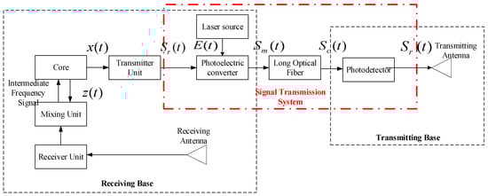
Figure 18.
The principle diagram of the dual-station RCS testing system.
Via analysis in conjunction with Figure 2, it can be gleaned that for a series of n frequency incrementation pulses with a carrier frequency of , the transmission of a specific pulse can be represented as follows:
where is the base frequency, which can be set according to the testing requirements, with the test system covering a frequency range of 1–40 GHz; is the inter-pulse frequency increment, set to 1 MHz; is the pulse width, determined by the maximum size of the target; and is the pulse repetition period, determined by the distance to the target. The target echo signal can be represented as follows:
where , is the target distance, and is the speed of light. The signal generated by agile frequency signal source 2 is as follows:
where one path, after mixing with signal , yields the reference intermediate frequency (IF) signal , while the other path, after mixing with the echo signal , produces signal :
After undergoing a series of processes including sampling, digital phase locking, quadrature digital down-conversion, and baseband signal post-processing, signals and yield the processed result :
Each pulse corresponds to a result, , and the system emits 30 pulses per measurement. As a result, a series of 30 echo information samples was obtained. Performing an IDFT on the echo data yielded the target’s distance and position information, i.e., the one-dimensional image. Next, the region of interest was centered around the target position, with zero-padding applied before performing a DFT. The frequency domain data were then used to compute the power spectrum of the echo, which allowed for the calculation of the target’s RCS value.
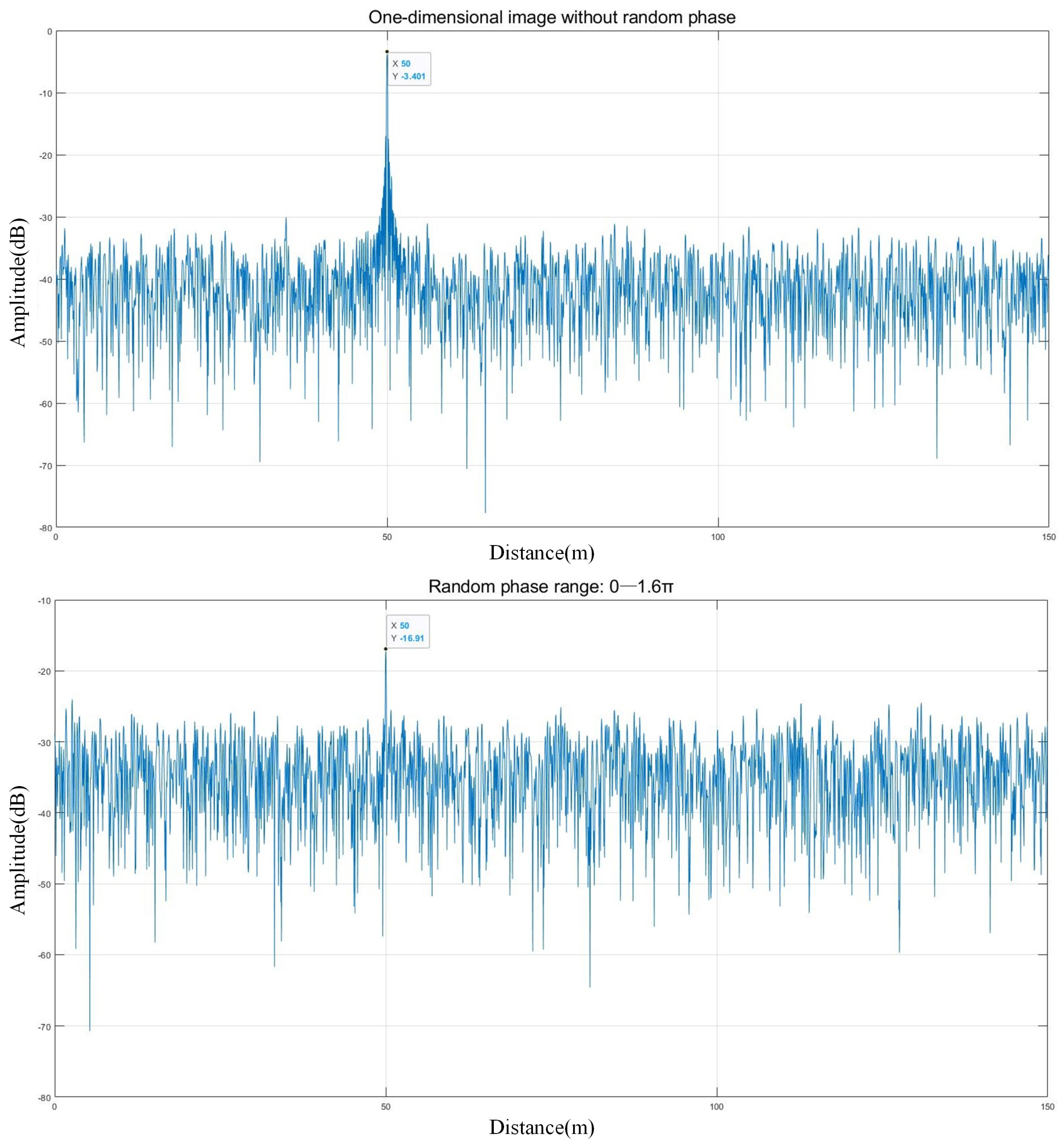
According to the system specifications, the transmission power of the system needs to reach at least to meet the testing requirements. Before introducing the long-distance signal transmission system, the system’s achieved transmission power was . Therefore, as long as the loss introduced by the signal transmission system is within , the requirements will be met. As indicated by the previous test results, the system not only did not undergo attenuation but also provided a gain of at least . Thus, its integration would not affect the overall transmission power of the system. Moreover, the results shown in Figure 19 indicate that the positional information in the one-dimensional image is only obscured when the introduced random phase error reaches around . In the test results, the phase error of the signal transmission system is less than 3 degrees (), which meets the required specifications.
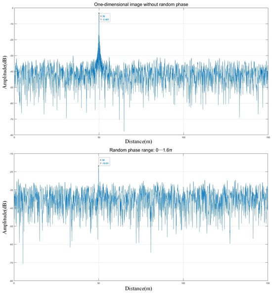
Figure 19.
The impact of random phase error on the one-dimensional image ().
Finally, after integrating the optoelectronic conversion system into the entire bistatic RCS testing system, we completed the measurement of the target’s RCS. Due to the lack of a physical vehicle or model, we selected a standard metal sphere as the test target. The metal sphere had a radius of approximately meters, and the RCS value for a sphere of this size is around . The testing environment is shown in Figure 20.

Figure 20.
Scenes depicting the RCS test.
The frequency chosen for the test was 10 GHz, with elevation angles of 0°, 45°, and 90° and horizontal angles ranging from −45° to 45°. The final measurement results are shown in Figure 21. From the figure, it can be gleaned that the measurement results differ from the theoretical value of by no more than 0.1 dB, indicating that the introduction of the optoelectronic conversion system did not affect the accuracy of the RCS measurement.

Figure 21.
RCS test results.
5. Conclusions
Combining an RCS with multipath effects allows a more detailed consideration of the scattering process when electromagnetic waves encounter obstacles, which is beneficial for improving the accuracy of multipath channel modeling. To achieve more accurate RCS measurements, we designed a signal transmission system between the bases of a bistatic RCS measurement system to achieve time synchronization between the bases. The operating frequency of the system can cover 1–40 GHz and remains linear, ensuring the phase coherence of the entire RCS testing system. The accompanying upper computer software for the system extracts amplitude and phase information from the received echo signals. After computational processing, the target’s RCS, one-dimensional image, and two-dimensional image can be obtained. However, the system currently only reaches the stage where it can function normally. In upcoming work, we will try to improve the accuracy of the testing system. Specific efforts will include reducing or eliminating the coupling between the test target and the ground during testing, minimizing the impact of environmental noise on the test results, and incorporating near-field-to-far-field transformation theory in data processing. The more accurate the RCS values obtained by the testing system, the higher the accuracy of multipath channel modeling.
Future research will focus on integrating RCS scattering characteristics with wireless communication in both vehicular networks and UAV communication systems. With this approach, we aim to incorporate more detailed scattering effects from vehicles and drones into channel modeling, thereby achieving greater accuracy [32].
Author Contributions
Conceptualization, T.H.; methodology, Y.H.; validation, Z.C. and P.L.; investigation, Y.H.; resources, Z.C. and P.L.; writing—original draft, Y.H.; writing—review and editing, T.H. and Y.W.; visualization, Y.H.; supervision, T.H.; project administration, T.H. All authors have read and agreed to the published version of the manuscript.
Funding
The work conducted by Tao Hong is funded by the National Natural Science Foundation of China [№ 3F72F5D9].
Institutional Review Board Statement
Not applicable.
Informed Consent Statement
Not applicable.
Data Availability Statement
The original contributions presented in the study are included in the article; further inquiries can be directed to the corresponding author.
Conflicts of Interest
The authors declare no conflicts of interest. The company had no role in the design of the study; in the collection, analyses, or interpretation of data; in the writing of the manuscript; or in the decision to publish the results.
References
- Andrews, J.G.; Buzzi, S.; Choi, W.; Hanly, S.V.; Lozano, A.; Soong, A.C.; Zhang, J.C. What will 5G be? IEEE J. Sel. Areas Commun. 2014, 32, 1065–1082. [Google Scholar] [CrossRef]
- Hirata, K.; Hiraguri, T.; Kimura, T.; Matsuda, T.; Imai, T.; Hirokawa, J.; Maruta, K.; Ujigawa, S. Study on Drone Handover Methods Suitable for Multipath Interference Due to Obstacles. Drones 2024, 8, 32. [Google Scholar] [CrossRef]
- Ali, S.; Abu-Samah, A.; Abdullah, N.F.; Kamal, N.L.M. Propagation Modeling of Unmanned Aerial Vehicle (UAV) 5G Wireless Networks in Rural Mountainous Regions Using Ray Tracing. Drones 2024, 8, 334. [Google Scholar] [CrossRef]
- Pokhrel, S.R.; Mandjes, M. Internet of Drones: Improving multipath TCP over WiFi with federated multi-armed bandits for limitless connectivity. Drones 2022, 7, 30. [Google Scholar] [CrossRef]
- Güldenring, J.; Gorczak, P.; Eckermann, F.; Patchou, M.; Tiemann, J.; Kurtz, F.; Wietfeld, C. Reliable long-range multi-link communication for unmanned search and rescue aircraft systems in beyond visual line of sight operation. Drones 2020, 4, 16. [Google Scholar] [CrossRef]
- Wang, S.; Gao, S.; Qin, F.; Yang, W. A Decomposition-Based Analysis of Wireless Multipath Channel with Full-Wave Simulation. IEEE Antenn. Wirel. Pr. 2022, 21, 1615–1619. [Google Scholar] [CrossRef]
- Clarke, R.H. A statistical theory of mobile-radio reception. Bell Syst. Tech. J. 1968, 47, 957–1000. [Google Scholar] [CrossRef]
- Almesaeed, R.; Ameen, A.S.; Doufexi, A.; Dahnoun, N.; Nix, A.R. A comparison study of 2D and 3D ITU channel model. In Proceedings of the 2013 IFIP Wireless Days (WD), Valencia, Spain, 13–15 November 2013. [Google Scholar]
- Samimi, M.K.; Rappaport, T.S. 3-D millimeter-wave statistical channel model for 5G wireless system design. IEEE Trans. Microw. Theory Tech. 2016, 64, 2207–2225. [Google Scholar] [CrossRef]
- Gao, M.; Wei, Y.; Guo, L.; Li, K. Atmospheric Duct 3D Propagation Model of Electromagnetic Wave Based on Ray Tracing Method. In Proceedings of the 2021 13th International Symposium on Antennas, Propagation and EM Theory (ISAPE), Zhuhai, China, 1–4 December 2021. [Google Scholar]
- Chang, Y.; Baek, S.; Hur, S.; Mok, Y.; Lee, Y. A novel dual-slope mm-Wave channel model based on 3D ray-tracing in urban environments. In Proceedings of the 2014 IEEE 25th Annual International Symposium on Personal, Indoor, and Mobile Radio Communication (PIMRC), Washington, DC, USA, 2–5 September 2014. [Google Scholar]
- Guan, K.; Lin, X.; He, D.; Ai, B.; Zhong, Z.; Zhao, Z.; Miao, D.; Guan, H.; Kürner, T. Scenario modules and ray-tracing simulations of millimeter wave and terahertz channels for smart rail mobility. In Proceedings of the 2017 11th European Conference on Antennas and Propagation (EUCAP), Paris, France, 19–24 March 2017. [Google Scholar]
- Jiang, Y.; Wang, M.; Ren, S. Modeling and experimental verification of space-time multipath wireless channel based on ray tracing. In Proceedings of the 2021 6th International Conference on Intelligent Computing and Signal Processing (ICSP), Xi’an, China, 9–11 April 2021. [Google Scholar]
- Chen, Y.; Li, Y.; Han, C.; Yu, Z.; Wang, G. Channel Measurement and Ray-Tracing-Statistical Hybrid Modeling for Low-Terahertz Indoor Communications. IEEE Trans. Wirel. Commun. 2021, 20, 8163–8176. [Google Scholar] [CrossRef]
- Wang, Y.; Cao, H.; Jin, Y.; Zhou, Z.; Wang, Y.; Huang, J.; Li, Y.; Huang, J.; Wang, C.X. An SBR Based Ray Tracing Channel Modeling Method for THz and Massive MIMO Communications. In Proceedings of the 2022 IEEE 96th Vehicular Technology Conference (VTC2022-Fall), London, UK, 1–6 September 2022. [Google Scholar]
- Nguyen, A.H.; Rath, M.; Leitinger, E.; Nguyen, K.V.; Witrisal, K. Gaussian process modeling of specular multipath components. Appl. Sci. 2020, 10, 5216. [Google Scholar] [CrossRef]
- Ding, R.; Wang, Z.; Jiang, L.; Zheng, S. Radar target localization with multipath exploitation in dense clutter environments. Appl. Sci. 2023, 13, 2032. [Google Scholar] [CrossRef]
- Wang, Q.; Chen, M.; Liu, J.; Lin, Y.; Li, K.; Yan, X.; Zhang, C. 1D-CLANet: A Novel Network for NLoS Classification in UWB Indoor Positioning System. Appl. Sci. 2024, 14, 7609. [Google Scholar] [CrossRef]
- Fawky, A.; Mohammed, M.; El-Hadidy, M.; Kaiser, T. UWB chipless RFID system performance based on real world 3D-deterministic channel model and ZF equalization. In Proceedings of the 8th European Conference on Antennas and Propagation (EuCAP 2014), The Hague, The Netherlands, 6–11 April 2014. [Google Scholar]
- Ge, D.; Wei, B. Electromagnetic Wave Theory; Science Press: Beijing, China, 2011. [Google Scholar]
- Richards, M.A. Fundamentals of Radar Signal Processing, 2nd ed.; Routledge: New York, NY, USA, 2005. [Google Scholar]
- Stimson, G.W. Stimson’s Introduction to Airborne Radar: Third Edition. J. Electron. Def. 2014, 37, 45. [Google Scholar]
- Shi, J.; Hu, G.; Zhu, S.; Luo, Y. Analysis and Progress of Radar Anti Stealth Technology. Mod. Def. Technol. 2015, 43, 124–130. [Google Scholar]
- Cui, J.; Ming, G.; Wang, F.; Li, J.; Wang, P.; Kang, S.; Zhao, F.; Zhong, D.; Mei, G. Realization of a Rubidium Atomic Frequency Standard with Short-Term Stability in 10−14 τ−1/2 Level. In Proceedings of the IEEE Transactions on Instrumentation and Measurement, New York, NY, USA, 1 January 2024. [Google Scholar]
- Sinatkas, G.; Christopoulos, T.; Tsilipakos, O.; Kriezis, E.E. Electro-optic modulation in integrated photonics. J. Appl. Phys. 2021, 130, 10901. [Google Scholar] [CrossRef]
- Yamada, E.; Ohki, A.; Kikuchi, N.; Shibata, Y.; Yasui, T.; Watanabe, K.; Ishii, H.; Iga, R.; Oohashi, H. Full C-band 40-Gbit/s DPSK tunable transmitter module developed by hybrid integration of tunable laser and InP npin Mach-Zehnder modulator. In Proceedings of the Optical Fiber Communication Conference, San Diego, CA, USA, 21–25 March 2010; Optica Publishing Group: Washington, DC, USA, 2010. [Google Scholar]
- Kikuchi, N.; Sanjoh, H.; Shibata, Y.; Tsuzuki, K.; Sato, T.; Yamada, E.; Ishibashi, T.; Yasaka, H. 80-Gbit/s InP DQPSK modulator with an npin structure. In Proceedings of the 33rd European Conference and Exhibition of Optical Communication, Berlin, Germany, 16–20 September 2007. [Google Scholar]
- Winzer, P.J.; Essiambre, R.J. Advanced modulation formats for high-capacity optical transport networks. J. Lightw. Technol. 2006, 24, 4711–4728. [Google Scholar] [CrossRef]
- Yang, H.; Crowley, M.; Marraccini, P.J.; Morrissey, P.E.; Li, Y.; Gao, L.; Corbett, B.; Peters, F.H. 50Gb/s InP-base Mach-Zehnder modulator. In Proceedings of the 2017 International Topical Meeting on Microwave Photonics (MWP), Beijing, China, 23–26 October 2017. [Google Scholar]
- Brast, T.; Kaiser, R.; Velthaus, K.O.; Gruner, M.; Maul, B.; Hamacher, M.; Hoffmann, D.; Schell, M. Monolithic 100 Gb/s twin-IQ Mach-Zehnder modulators for advanced hybrid high-capacity transmitter boards. In Proceedings of the Optical Fiber Communication Conference, Los Angeles, CA, USA, 6–10 March 2011. [Google Scholar]
- Zhang, J.; Yu, J.; Li, X.; Wang, K.; Zhou, W.; Xiao, J.; Zhao, L.; Pan, X.; Liu, B.; Xin, X. 200 Gbit/s/λ PDM-PAM-4 PON system based on intensity modulation and coherent detection. J. Opt. Commun. Netw. 2020, 12, A1–A8. [Google Scholar] [CrossRef]
- Qi, W.; Bian, J.; Wang, Z.; Liu, W. A Novel UAV Air-to-Air Channel Model Incorporating the Effect of UAV Vibrations and Diffuse Scattering. Drones 2024, 8, 194. [Google Scholar] [CrossRef]

Disclaimer/Publisher’s Note: The statements, opinions and data contained in all publications are solely those of the individual author(s) and contributor(s) and not of MDPI and/or the editor(s). MDPI and/or the editor(s) disclaim responsibility for any injury to people or property resulting from any ideas, methods, instructions or products referred to in the content. |
© 2024 by the authors. Licensee MDPI, Basel, Switzerland. This article is an open access article distributed under the terms and conditions of the Creative Commons Attribution (CC BY) license (https://creativecommons.org/licenses/by/4.0/).