
Study of the Sliding Friction Coefficient of Different-Size Elements in Discrete Element Method Based on an Experimental Method


Abstract
1. Introduction
2. Experimental Method
3. Simulation Model
4. Results and Discussion
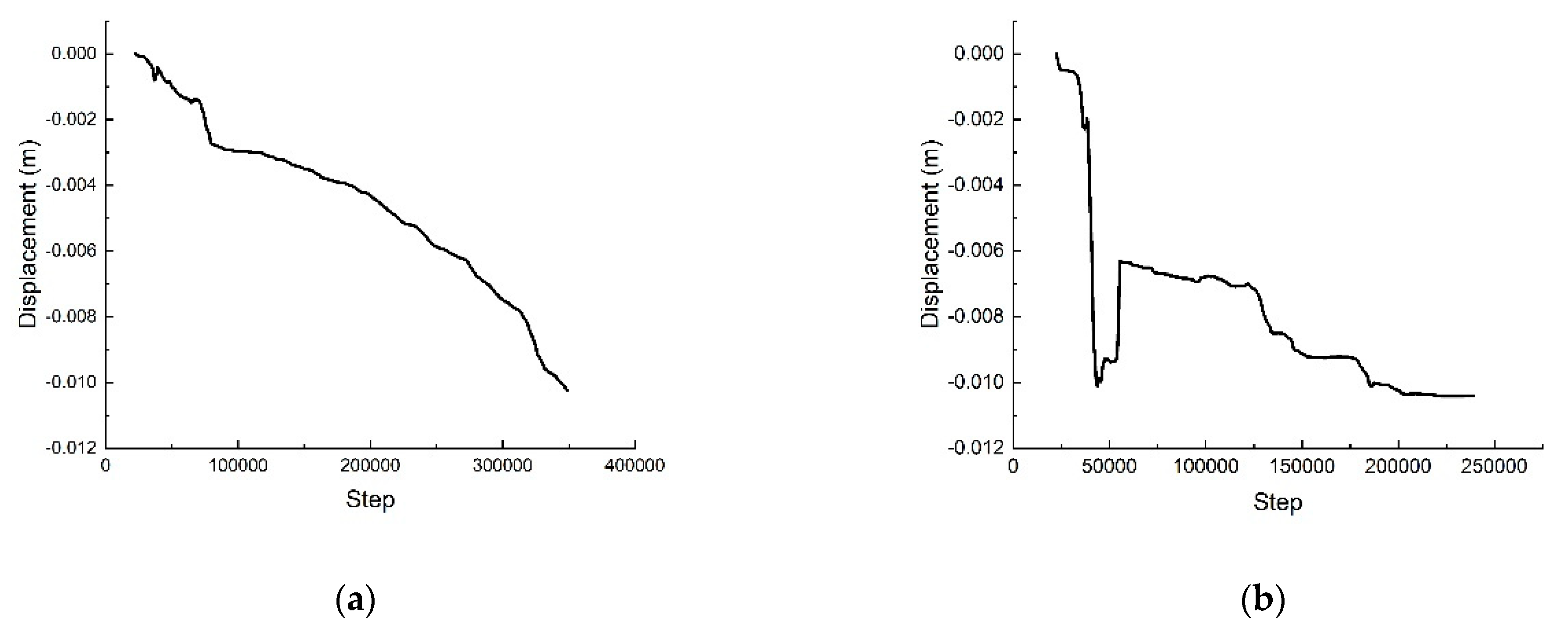
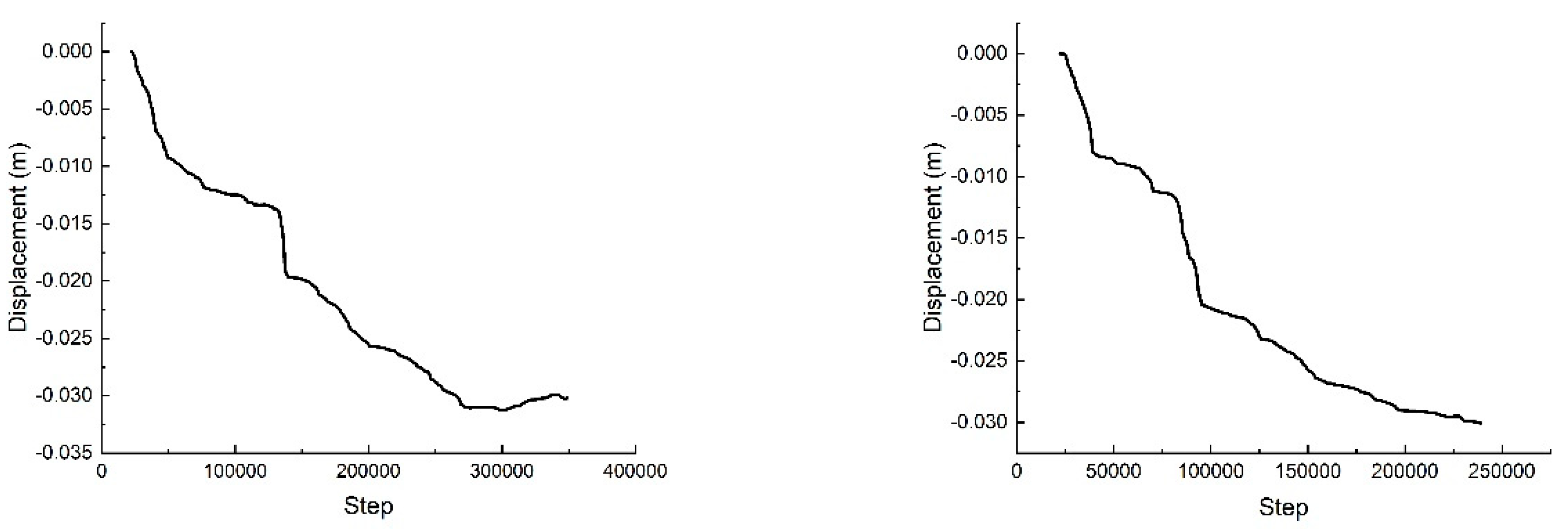
- (1)
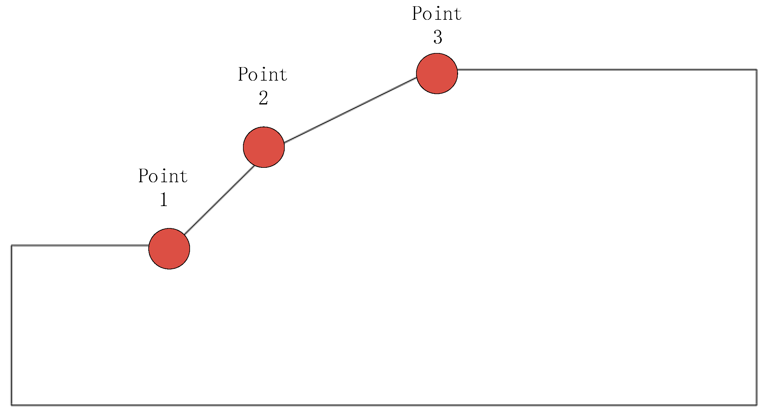
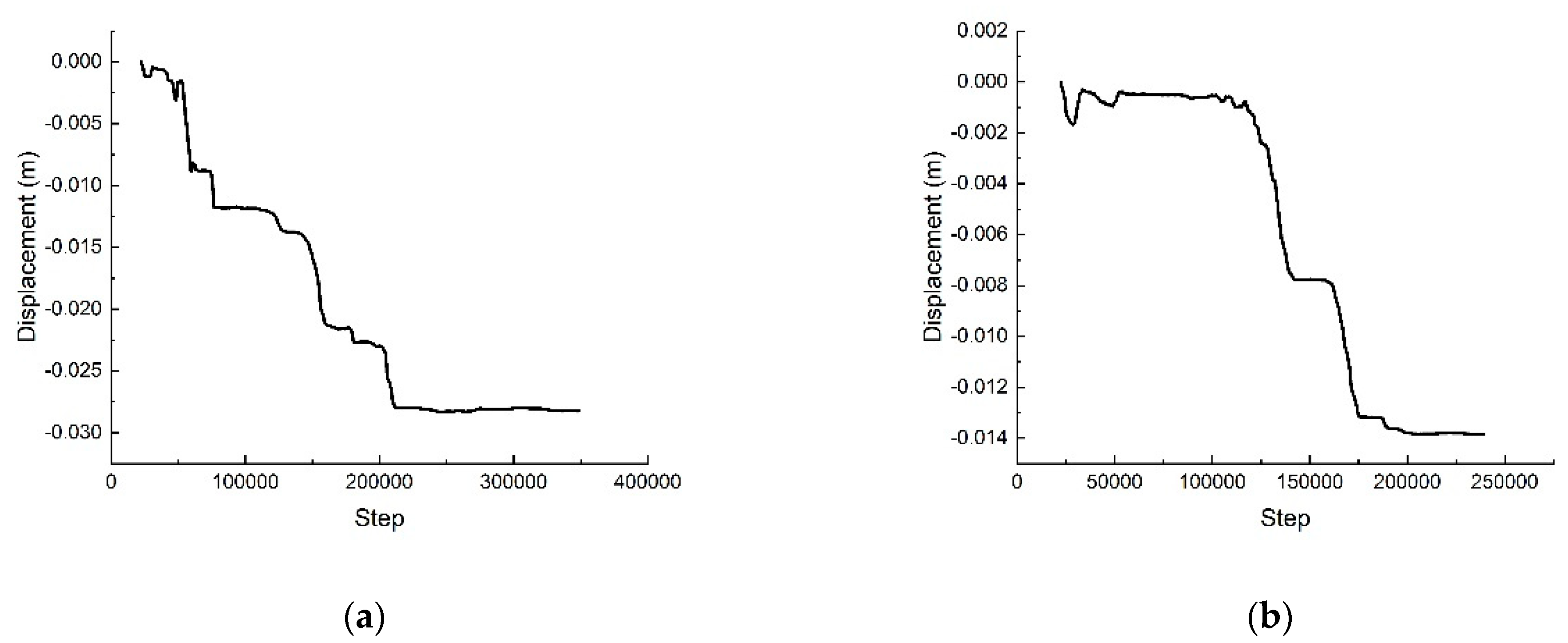
- The horizontal displacement trend of each measuring point is roughly the same: each measuring point develops in the direction away from the slope, showing a trend of gradual sliding. The displacement diagrams of measuring points 1 and 2 clearly fluctuate. The reason for this is that the elements constituting the slope model are discrete, and there is a certain gap between the circular elements. During the development of the sliding surface, there is a certain probability that a smaller element will fall into the gap due to gravity. However, the overall development trend of each measuring point of the two models is basically the same.
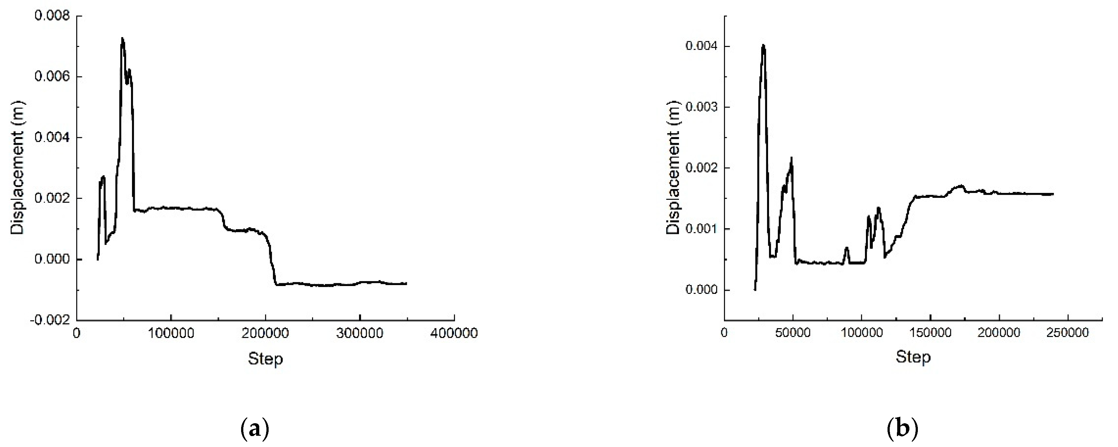
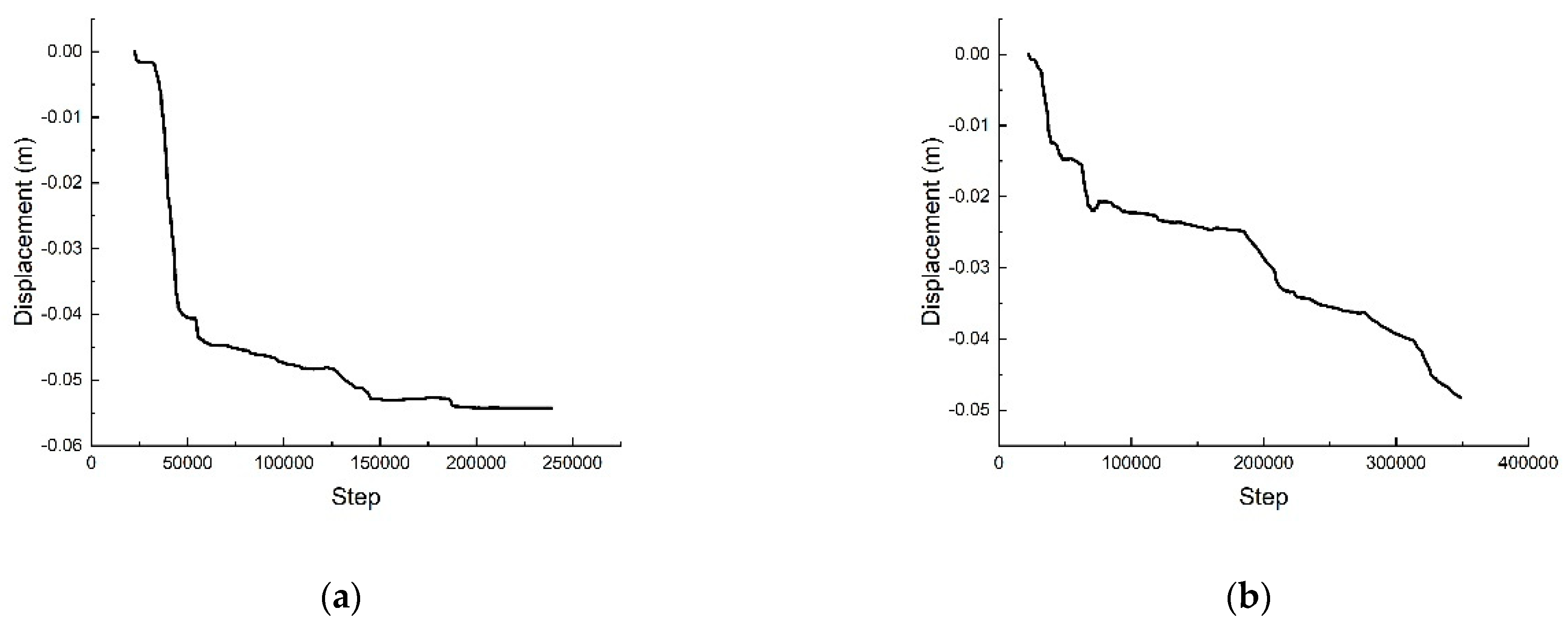
- (2)
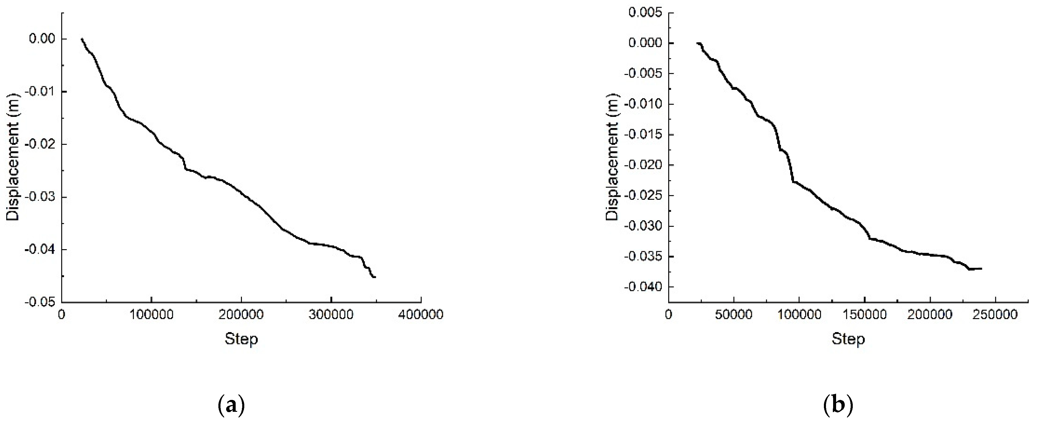
- The vertical displacement trend of each measuring point is the same: each measuring point develops in the direction of deviation from the slope, showing a trend of gradual sliding. The displacement diagram of measuring point 2 has clear fluctuations due to reasons similar to those above, owing to the discrete elements and different-sized elements. However, the overall development trend of each measuring point of the two models is basically the same.
- (3)
- By comparing the two DEM slope models, it can be seen that the displacement of the DEM model embedded into the sliding friction coefficient algorithm is larger. The reason for this is that for larger-size elements, the contact information between a single sliding friction coefficient and the DEM elements embedded in the sliding friction coefficient algorithm is basically the same. For smaller-sized elements, the sliding friction coefficient between the DEM elements with a single sliding friction coefficient will be larger, resulting in a change in contact information. The contact information is related to many DEM parameters. Although the sliding friction coefficient algorithm will increase the calculation time, the calculation accuracy can be improved from a mechanical point of view.
5. Conclusions
- (1)
- We compared and analyzed the horizontal displacement and vertical displacement of an original DEM model and a DEM slope model embedded with a sliding friction coefficient algorithm. The sliding friction coefficient has an influence on the calculation of the discrete element model. That is, in the DEM model, different sliding friction coefficients should be set between different-sized elements to improve the accuracy of the DEM simulation.
- (2)
- By comparing and analyzing the changing horizontal and vertical displacement trends of each measuring point of the original DEM model and the DEM model with the sliding friction coefficient algorithm, we found that the two have the same trend at each measuring point. Each measuring point develops in the direction away from the slope, showing a trend of gradual sliding.
- (3)
- There are some fluctuations in the displacement curve. The reason for this is that the elements are discrete, and there is a certain gap between the elements. During the development of the sliding surface, there is a certain probability that smaller elements will fall into the gap due to gravity. However, the overall development trend of each measuring point of the two models is basically the same.
Author Contributions
Funding
Institutional Review Board Statement
Informed Consent Statement
Data Availability Statement
Acknowledgments
Conflicts of Interest
References
- Kasai, M.; Ikeda, M.; Asahina, T.; Fujisawa, K. LiDAR-derived DEM evaluation of deep-seated landslides in a steep and rocky region of Japan. Geomorphology 2009, 113, 57–69. [Google Scholar] [CrossRef]
- Mao, J.; Zhao, L.; Di, Y.; Liu, X.; Xu, W. A resolved CFD–DEM approach for the simulation of landslides and impulse waves. Comput. Methods Appl. Mech. Eng. 2020, 359, 112750. [Google Scholar] [CrossRef]
- Bao, X.; Wu, H.; Xiong, H.; Chen, X. Particle shape effects on submarine landslides via CFD-DEM. Ocean Eng. 2023, 284, 115140. [Google Scholar] [CrossRef]
- Tappin, D.R. Digital elevation models in the marine domain: Investigating the offshore tsunami hazard from submarine landslides. Geol. Soc. Lond. Spec. Publ. 2010, 345, 81–101. [Google Scholar] [CrossRef]
- Teufelsbauer, H.; Wang, Y.; Chiou, M.-C.; Wu, W. Flow–obstacle interaction in rapid granular avalanches: DEM simulation and comparison with experiment. Granul. Matter 2009, 11, 209–220. [Google Scholar] [CrossRef]
- Kalokhe, A.; Patil, D. Study of Particle Avalanches: A Discrete Element Method Approach. In Proceedings of the Conference on Fluid Mechanics and Fluid Power, Pilani, India, 27–29 December 2021; pp. 49–54. [Google Scholar]
- Zhang, Y.; Li, L. Introduction and implementation of fluid forces in a DEM code for simulating particle settlement in fluids. Powder Technol. 2024, 433, 119238. [Google Scholar] [CrossRef]
- Ahmadi, H.; Sizkow, S.F. Numerical analysis of ground improvement effects on dynamic settlement of uniform sand using DEM. SN Appl. Sci. 2020, 2, 689. [Google Scholar] [CrossRef]
- Aranson, I.S.; Tsimring, L.S. Patterns and collective behavior in granular media: Theoretical concepts. Rev. Mod. Phys. 2006, 78, 641–692. [Google Scholar] [CrossRef]
- Seiden, G.; Thomas, P.J. Complexity, segregation, and pattern formation in rotating-drum flows. Rev. Mod. Phys. 2011, 83, 1323–1365. [Google Scholar] [CrossRef]
- Cundall, P.A. A computer model for simulating progressive, large-scale movement in blocky rock system. In Proceedings of the International Symposium on Rock Mechanics, Nancy, France, 4–6 October 1971; pp. 129–136. [Google Scholar]
- Cundall, P.A.; Strack, O.D.L. A discrete numerical model for granular assemblies. Géotechnique 1979, 29, 47–65. [Google Scholar] [CrossRef]
- Cundall, P. Computer simulations of dense sphere assemblies. In Studies in Applied Mechanics; Elsevier: Amsterdam, The Netherlands, 1988; Volume 20, pp. 113–123. [Google Scholar]
- Ting, J.M.; Khwaja, M.; Meachum, L.R.; Rowell, J.D. An ellipse-based discrete element model for granular materials. Int. J. Numer. Anal. Methods Geomech. 1993, 17, 603–623. [Google Scholar] [CrossRef]
- Ting, J.M.; Meachum, L.; Rowell, J.D. Effect of particle shape on the strength and deformation mechanisms of ellipse-shaped granular assemblages. Eng. Comput. 1995, 12, 99–108. [Google Scholar] [CrossRef]
- Ng, T.-T. Numerical simulations of granular soil using elliptical particles. Comput. Geotech. 1994, 16, 153–169. [Google Scholar] [CrossRef]
- Lin, X.; Ng, T.-T. A three-dimensional discrete element model using arrays of ellipsoids. Geotechnique 1997, 47, 319–329. [Google Scholar] [CrossRef]
- Chen, H.; Zhao, S.; Zhou, X. DEM investigation of angle of repose for super-ellipsoidal particles. Particuology 2020, 50, 53–66. [Google Scholar] [CrossRef]
- Liu, Z.; Zhao, Y. Multi-super-ellipsoid model for non-spherical particles in DEM simulation. Powder Technol. 2020, 361, 190–202. [Google Scholar] [CrossRef]
- Liu, P.; Liu, J.; Du, H.; Yin, Z. A method of normal contact force calculation between spherical particles for discrete element method. In Proceedings of the 1st International Conference on Mechanical System Dynamics (ICMSD 2022), Nanjing, China, 24–27 August 2022; pp. 45–52. [Google Scholar]
- Yin, Z.; Liu, J.; Du, H.; Liu, P. An improved ellipsoid-ellipsoid discrete element framework algorithm design and code development. In Proceedings of the 1st International Conference on Mechanical System Dynamics (ICMSD 2022), Nanjing, China, 24–27 August 2022; pp. 76–82. [Google Scholar]
- Mori, Y.; Sakai, M. Advanced DEM simulation on powder mixing for ellipsoidal particles in an industrial mixer. Chem. Eng. J. 2022, 429, 132415. [Google Scholar] [CrossRef]
- Hoorijani, H.; Esgandari, B.; Zarghami, R.; Sotudeh-Gharebagh, R.; Mostoufi, N. Predictive modeling of mixing time for super-ellipsoid particles in a four-bladed mixer: A DEM-based approach. Powder Technol. 2023, 430, 119009. [Google Scholar] [CrossRef]
- Xia, X.; Zhou, L.; Ma, H.; Xie, C.; Zhao, Y. Reliability study of super-ellipsoid DEM in representing the packing structure of blast furnace. Particuology 2022, 70, 72–81. [Google Scholar] [CrossRef]
- Chang, J.; Wang, W.; Zhao, M.; Liu, K. Experimental study and simulation analysis on friction behavior of a mechanical surface sliding on hard particles. Proc. Inst. Mech. Eng. Part J J. Eng. Tribol. 2017, 231, 1371–1379. [Google Scholar] [CrossRef]
- Bek, M.; Gonzalez-Gutierrez, J.; Lopez, J.A.M.; Bregant, D.; Emri, I. Apparatus for measuring friction inside granular materials—Granular friction analyzer. Powder Technol. 2016, 288, 255–265. [Google Scholar] [CrossRef]
- Wang, W.; Zhang, J.; Yang, S.; Zhang, H.; Yang, H.; Yue, G. Experimental study on the angle of repose of pulverized coal. Particuology 2010, 8, 482–485. [Google Scholar] [CrossRef]
- Liu, P.; Liu, J.; Gao, S.; Wang, Y.; Zheng, H.; Zhen, M.; Zhao, F.; Liu, Z.; Ou, C.; Zhuang, R. Calibration of Sliding Friction Coefficient in DEM between Different Particles by Experiment. Appl. Sci. 2023, 13, 11883. [Google Scholar] [CrossRef]
- Wang, H.; Jia, P.; Wang, L.; Yun, F.; Wang, G.; Wang, X.; Liu, M. Research on the loading–unloading fractal contact model between two three-dimensional spherical rough surfaces with regard to friction. Acta Mech. 2020, 231, 4397–4413. [Google Scholar] [CrossRef]
- Shi, C.; Yang, W.; Yang, J.; Chen, X. Calibration of micro-scaled mechanical parameters of granite based on a bonded-particle model with 2D particle flow code. Granul. Matter 2019, 21, 38. [Google Scholar] [CrossRef]
- Sakaguchi, H.; Ozaki, E.; Igarashi, T. Plugging of the flow of granular materials during the discharge from a silo. Int. J. Mod. Phys. B 1993, 7, 1949–1963. [Google Scholar] [CrossRef]
- Iwashita, K.; Oda, M. Micro-deformation mechanism of shear banding process based on modified distinct element method. Powder Technol. 2000, 109, 192–205. [Google Scholar] [CrossRef]
- Markauskas, D.; Kačianauskas, R.; Džiugys, A.; Navakas, R. Investigation of adequacy of multi-sphere approximation of elliptical particles for DEM simulations. Granul. Matter 2010, 12, 107–123. [Google Scholar] [CrossRef]
- Popova, E.; Popov, V.L. The research works of Coulomb and Amontons and generalized laws of friction. Friction 2015, 3, 183–190. [Google Scholar] [CrossRef]
- Greenwood, J.A.; Tripp, J.H. The Elastic Contact of Rough Spheres. J. Appl. Mech. 1967, 34, 153–159. [Google Scholar] [CrossRef]
- Ghatrehsamani, S.; Akbarzadeh, S. Predicting the wear coefficient and friction coefficient in dry point contact using continuum damage mechanics. Proc. Inst. Mech. Eng. Part J J. Eng. Tribol. 2019, 233, 447–455. [Google Scholar] [CrossRef]
- Ghatrehsamani, S.; Akbarzadeh, S.; Khonsari, M. Experimentally verified prediction of friction coefficient and wear rate during running-in dry contact. Tribol. Int. 2022, 170, 107508. [Google Scholar] [CrossRef]
- Zhao, Y.; Maietta, D.M.; Chang, L. An asperity microcontact model incorporating the transition from elastic deformation to fully plastic flow. J. Tribol. 2000, 122, 86–93. [Google Scholar] [CrossRef]
- Hurtado, J.A.; Kim, K.S. Scale effects in friction of single–asperity contacts. I. From concurrent slip to single–dislocation–assisted slip. Proc. R. Soc. Lond. Ser. A Math. Phys. Eng. Sci. 1999, 455, 3363–3384. [Google Scholar] [CrossRef]
- Asaf, Z.; Rubinstein, D.; Shmulevich, I. Determination of discrete element model parameters required for soil tillage. Soil Tillage Res. 2007, 92, 227–242. [Google Scholar] [CrossRef]
- Adams, G.G.; Müftü, S.; Azhar, N.M. A scale-dependent model for multi-asperity contact and friction. J. Tribol. 2003, 125, 700–708. [Google Scholar] [CrossRef]
- Zhuravlev, V. The model of dry friction in the problem of the rolling of rigid bodies. J. Appl. Math. Mech. 1998, 62, 705–710. [Google Scholar] [CrossRef]
- Wang, L.; Xiang, Y. Elastic-plastic contact analysis of a deformable sphere and a rigid flat with friction effect. Adv. Mater. Res. 2013, 644, 151–156. [Google Scholar] [CrossRef]
- Chen, Z.; Etsion, I. Model for the static friction coefficient in a full stick elastic-plastic coated spherical contact. Friction 2019, 7, 613–624. [Google Scholar] [CrossRef]
- Cheng, Y.M.; Lansivaara, T.; Wei, W. Two-dimensional slope stability analysis by limit equilibrium and strength reduction methods. Comput. Geotech. 2007, 34, 137–150. [Google Scholar] [CrossRef]


| Label | Average Diameter (mm) | Standard Deviation (mm) | Number of Particles |
|---|---|---|---|
| S3 | 29.62 | 0.49 | 32 |
| S3.5 | 34.69 | 0.38 | 32 |
| S4 | 40.08 | 0.45 | 32 |
| S4.5 | 45.02 | 0.40 | 32 |
| S5 | 49.72 | 0.39 | 32 |
| S5.5 | 55.26 | 0.42 | 32 |
| S6 | 60.12 | 0.42 | 32 |
| Label | S3 | S3.5 | S4 | S4.5 | S5 | S5.5 | S6 |
|---|---|---|---|---|---|---|---|
| S3 | 0.46 | 0.47 | 0.48 | 0.49 | 0.49 | 0.50 | 0.51 |
| S3.5 | 0.47 | 0.48 | 0.48 | 0.49 | 0.50 | 0.50 | 0.52 |
| S4 | 0.48 | 0.48 | 0.50 | 0.50 | 0.51 | 0.52 | 0.53 |
| S4.5 | 0.49 | 0.49 | 0.50 | 0.50 | 0.52 | 0.52 | 0.53 |
| S5 | 0.49 | 0.50 | 0.51 | 0.52 | 0.53 | 0.54 | 0.56 |
| S5.5 | 0.50 | 0.50 | 0.52 | 0.52 | 0.54 | 0.57 | 0.58 |
| S6 | 0.51 | 0.52 | 0.53 | 0.53 | 0.56 | 0.58 | 0.58 |
| Label | Symbol | Value |
|---|---|---|
| Young’s modulus | E | 14.0 MPa |
| Poisson’s ratio | ν | 0.3 |
| Gravity | g | 9.8 m/s2 |
| Friction coefficient | μs | 0.58 |
| Measuring Point | Original Model (mm) | Modified Model (mm) |
|---|---|---|
| Horizontal displacement of point 1 | −1.4 | −2.7 |
| Vertical displacement of point 1 | −3.7 | −4.6 |
| Horizontal displacement of point 2 | −0.1 | −0.1 |
| Vertical displacement of point 2 | −0.1 | 0.2 |
| Horizontal displacement of point 3 | −3.0 | −3.0 |
| Vertical displacement of point 3 | −4.8 | −5.4 |
Disclaimer/Publisher’s Note: The statements, opinions and data contained in all publications are solely those of the individual author(s) and contributor(s) and not of MDPI and/or the editor(s). MDPI and/or the editor(s) disclaim responsibility for any injury to people or property resulting from any ideas, methods, instructions or products referred to in the content. |
© 2024 by the authors. Licensee MDPI, Basel, Switzerland. This article is an open access article distributed under the terms and conditions of the Creative Commons Attribution (CC BY) license (https://creativecommons.org/licenses/by/4.0/).
Share and Cite
Liu, P.; Rui, Y.; Wang, Y. Study of the Sliding Friction Coefficient of Different-Size Elements in Discrete Element Method Based on an Experimental Method. Appl. Sci. 2024, 14, 8802. https://doi.org/10.3390/app14198802
Liu P, Rui Y, Wang Y. Study of the Sliding Friction Coefficient of Different-Size Elements in Discrete Element Method Based on an Experimental Method. Applied Sciences. 2024; 14(19):8802. https://doi.org/10.3390/app14198802
Chicago/Turabian StyleLiu, Pengcheng, Yi Rui, and Yue Wang. 2024. "Study of the Sliding Friction Coefficient of Different-Size Elements in Discrete Element Method Based on an Experimental Method" Applied Sciences 14, no. 19: 8802. https://doi.org/10.3390/app14198802
APA StyleLiu, P., Rui, Y., & Wang, Y. (2024). Study of the Sliding Friction Coefficient of Different-Size Elements in Discrete Element Method Based on an Experimental Method. Applied Sciences, 14(19), 8802. https://doi.org/10.3390/app14198802