Robust H_∞ Control for Autonomous Underwater Vehicle’s Time-Varying Delay Systems under Unknown Random Parameter Uncertainties and Cyber-Attacks

Abstract

This paper investigates robust $H_{\infty }$-based control for autonomous underwater vehicle (AUV) systems under time-varying delay, model uncertainties, and cyber-attacks. Sensor and actuator cyber-attacks can cause faults in the overall AUV system. In addition, the behavior of the system can be affected by the presence of complexities, such as unknown random uncertainties that occur in system modeling. In this paper, the robustness against unpredictable random uncertainties is investigated by considering unknown but norm-bounded (UBB) random uncertainties. By constructing a proper Lyapunov–Krasovskii functional (LKF) and using linear matrix inequality (LMI) techniques, new stability criteria in the form of LMIs are derived such that the AUV system is stable. Moreover, this work is novel in addressing robust $H_{\infty }$ control, which considers time-varying delay, cyber-attacks, and randomly occurring uncertainties for AUV systems. Finally, the effectiveness of the proposed results is demonstrated through two examples and their computer simulations.

1. Introduction

Autonomous underwater vehicles (AUVs) have become indispensable robotic devices for ocean exploration that carry out various military and civilian applications, including ocean floor surveying, oceanographic data gathering, minefield surveying, pipeline inspection, and anti-submarine warfare [1,2,3]. Research in underwater vehicles has been very active in the past few decades with the advancement of control, sensing, communication, and computing technologies. In practice, controlling the stability of AUV is a challenging task during underwater operations and time-varying disturbances [4], i.e., the payload, mass, dynamics, and buoyancy will change when performing different tasks. In addition, AUV suffers from marine environmental external disturbances, i.e., wakes, ocean currents [5,6], and unpredictable uncertainties [7,8,9].

In recent years, the security of autonomous marine vehicles has attracted much attention because attackers can access a set of sensors and actuator devices, modify their software or environment, and carry out coordinated attacks on the system design. In cyber-security, control technology has been widely applied, and it is well known that control performance depends on the quality of control input and sensor measurement signals [10]. Recently, sensor and actuator attacks were presented in adaptive neural dissipative control for Markovian jump cyber-physical systems [11], resilient control of cyber-physical systems [12], and cyber-attacks in industrial control systems [13]. A secure tracking control was developed in [14] to guarantee the prescribed security in systems with sensor and actuator attacks. Actuator saturation and probabilistic cyber-attacks were discussed in uncertain networked control systems [15]. The hybrid-driven-based resilient control for T-S fuzzy systems with time-delay and cyber-attack was investigated in [16].

The behavior of the system can be affected by complexities such as random uncertainties that occur during system modeling. These complexities are subject to random changes in complicated circumstances, exceptional environmental disturbances, random failures, modeling errors, varying geometry and material properties, repairs of system components, and so forth, which may occur in a probabilistic way. The appearance of parameter uncertainties often exhibits a random nature, because of unpredictable changes. As a result, the so-called randomly occurring uncertainty (ROU) is usually controlled by Bernoulli-distributed stochastic variables. In recent years, the concept of randomly occurring uncertainties has been investigated in [17,18].

Time-varying delay frequently occurs in AUV controls, and it may cause undesirable transient system responses, diminish system performance, and even lead to instability. References [19,20] discussed unknown uncertainties and time-varying delays in AUV systems. In recent years, the concept of time-varying delay and delays in vehicle systems has been investigated [21,22,23]. In [19,20], robustness against unpredictable uncertainties was investigated by considering unknown but norm-bounded (UBB) uncertainties. However, note that UBB random uncertainties were not handled in [19,20].

Inspired by [19,20], our paper addresses robustness against unpredictable random uncertainties by considering UBB random uncertainties. Moreover, we handle time-varying delay in AUV controls. However, to the best of our knowledge, cyber-attacks were not handled in the control of AUV systems. To the best of our knowledge, no papers are available on the stabilization of AUV systems with time-varying delay, randomly occurring uncertainties, and cyber-attacks.

In our paper, we design a robust $H_{\infty }$ control for autonomous underwater vehicle systems under time-varying delay, uncertain random models, and cyber-attacks. The AUV model and schematic of the AUV system in the presence of cyber-attacks and external disturbances are shown in Figure 1. The effectiveness of the proposed $H_{\infty }$ control is demonstrated by two examples and their computer simulations. Using computer simulations, we compare the performance of our robust $H_{\infty }$ control with controls in [19,20], and present the outperformance of the proposed $H_{\infty }$ control.

The remainder of this article is summarized as follows: Section 2 provides the problem formulation and preliminaries. Section 3 presents the stability of the proposed AUV systems. Section 4 provides two examples using the MATLAB R2023b Toolbox. Section 5 provides the conclusion of this paper.

2. Problem Formulation and Preliminaries

In this section, problem formulation, basic assumptions, definition, and lemma are given.

Notations: In this work, ${\mathbb{R}}^n$ and ${\mathbb{R}}^{n\times m}$ denotes the n-dimensional Euclidean real space, and the set of $n\times m$ real matrices; “T” is the superscript for matrix transposition; “(−1)” is the superscript for matrix inverse. In a symmetric matrix, the symmetric term is indicated by the symbol “∗”. The notation P > 0 (<0) indicates that positive definite (negative definite) symmetric matrix and “I” is the identity matrix with the proper dimension.

2.1. AUV System I with Time-Varying Delay

Motivated by [19], we consider the class of continuous-time linear uncertain time-varying delay systems of the form:

$$\begin{array}{c}\hfill \begin{array}{ccc}\dot{x}\left(t\right)& =\hfill & (A+\Delta A)x\left(t\right)+(A_d+\Delta A_d)x(t-\tau \left(t\right))+Bu\left(t\right)+B_{w}w\left(t\right),\hfill \\ y\left(t\right)& =\hfill & Cx\left(t\right),\hfill \\ x\left(t\right)& =\hfill & \varphi \left(t\right),t\in [-{\tau }_M,0],\hfill \end{array}\end{array}$$

(1)

where $x\left(t\right)\in {\mathbb{R}}^n$ is the state at time t, $u\left(t\right)\in {\mathbb{R}}^m$ is the control input, $w\left(t\right)\in {\mathbb{R}}^p$ is the external disturbance that belongs to ${\mathbb{L}}_2[0,+\infty )$, $y\left(t\right)\in {\mathbb{R}}^q$ is the measured output, and $\varphi \left(t\right)$ is the initial state condition. A, $A_d$, B, $B_w$, and C are known matrices of appropriate dimensions. $\tau \left(t\right)$ is a nonnegative time-varying delay affecting the system states, assumed to be bounded as $0\le {\tau }_m\le \tau \left(t\right)\le {\tau }_M$ and $\dot{\tau }\left(t\right)\le \mu <\infty$, where $\mu \in {\mathbb{R}}^{+}$. The state feedback controller can be designed and formulated as follows:

$$\begin{array}{c}\hfill u\left(t\right)=Kx\left(t\right)\end{array}$$

(2)

where K is the feedback control gain.

According to [19,20], $\Delta A$ and $\Delta A_d$ represent the UBB uncertainties in system (1) satisfying:

$$\begin{array}{c}\hfill \begin{array}{c}\Delta A=M_1\Delta \left(t\right)N_1,\Delta A_d=M_2\Delta \left(t\right)N_2\end{array}\end{array}$$

(3)

where $M_1$, $N_1$, $M_2$, and $N_2$ are known as constant matrices with appropriate dimensions and $\Delta \left(t\right)$ is an unknown matrix with Lebesgue measurable elements and satisfies $\Delta {\left(t\right)}^T\Delta \left(t\right)\le I$.

Note that the behavior of the system can be affected by the presence of complexities, such as random uncertainties that occur during the process of system modeling. The appearance of parameter uncertainties often exhibits a random nature, due to unpredictable changes. As a result, the ROU is usually controlled by Bernoulli-distributed stochastic variables. In recent years, the concept of randomly occurring uncertainties has been investigated [17,18].

In our paper, the randomly occurring UBB uncertainties are assumed to follow a Bernoulli distribution, which is expressed as follows:

$$\begin{array}{c}\hfill Prob\{\alpha \left(t\right)=1\}=\overline{\alpha },Prob\{\alpha \left(t\right)=0\}=1-\overline{\alpha },\end{array}$$

where $\overline{\alpha }\in [0,1]$ is a known constant. The stochastic variable $\alpha \left(t\right)\in \mathbb{R}$ is introduced to characterize the randomly occurring uncertainties.

Now, considering the randomly occurring uncertainties [17] and the sensor and actuator attacks [24] in system (1), we have the following formulation:

$$\begin{array}{c}\hfill \begin{array}{ccc}\dot{x}\left(t\right)& =\hfill & (A+\alpha \left(t\right)\Delta A)x\left(t\right)+(A_d+\alpha \left(t\right)\Delta A_d)x(t-\tau \left(t\right))\hfill \\ & & +B[u\left(t\right)+\beta \left(t\right){\chi }_a\left(t\right)]+B_{w}w\left(t\right),\hfill \\ y\left(t\right)& =\hfill & Cx\left(t\right)+\gamma \left(t\right){\chi }_s\left(t\right),\hfill \\ x\left(t\right)& =\hfill & \varphi \left(t\right),t\in [-{\tau }_M,0],\hfill \end{array}\end{array}$$

(4)

where $x\left(t\right)\in {\mathbb{R}}^n$ denotes the state vector affected by the actuator attack ${\chi }_a\left(t\right)$, $y\left(t\right)\in {\mathbb{R}}^q$ is the measurable output affected by the sensor attack ${\chi }_s\left(t\right)$, and nonlinear functions ${\chi }_a\left(t\right)$ and ${\chi }_s\left(t\right)$ are used to model the cyber signals inserted by attackers. The probability of the event that the system’s actuator or sensor has been affected by a cyber-attack is denoted by ${\overline{\chi }}_a\in [0,1]$ (or ${\overline{\chi }}_s\in [0,1]$).

According to [25], both $\beta \left(t\right)$ and $\gamma \left(t\right)$ are Markovian stochastic processes with the binary state (0 or 1), which satisfy the following probability:

$$\begin{array}{c}\hfill \begin{array}{c}E\left\{\beta \left(t\right)\right\}=Prob\{\beta \left(t\right)=1\}=\overline{\beta },\\ E\left\{\gamma \left(t\right)\right\}=Prob\{\gamma \left(t\right)=1\}=\overline{\gamma }.\end{array}\end{array}$$

(5)

where an actuator cyber-attack ${\chi }_a\left(t\right)$ (or a sensor cyber-attack ${\chi }_s\left(t\right)$) happens when event $\beta \left(t\right)=1$ (or $\gamma \left(t\right)=1$), which indicates that the actuator (or the sensor) of the system is the target of a cyber-attack. On the other hand, event $\beta \left(t\right)=0$ (or $\gamma \left(t\right)=0$) indicates that there is no cyber-attack on the actuator (or on the sensor). A cyber-attack on the system’s actuator (or sensor) is represented as $\overline{\beta }\in [0,1]$ (or $\overline{\gamma }\in [0,1]$), which indicates the possibility of the attack.

2.2. AUV System II with Time-Varying Delays

Motivated by [20], we consider the continuous-time linear uncertain time-varying delays system of the form:

$$\begin{array}{c}\hfill \begin{array}{ccc}\dot{x}\left(t\right)& =\hfill & (A+\alpha \left(t\right)\Delta A)x\left(t\right)+(A_d+\alpha \left(t\right)\Delta A_d)x(t-\tau \left(t\right))\hfill \\ & & +B[u\left(t\right)+\beta \left(t\right){\chi }_a\left(t\right)]+B_{d}u(t-\tau \left(t\right))+B_{w}w\left(t\right),\hfill \\ y\left(t\right)& =\hfill & Cx\left(t\right)+\gamma \left(t\right){\chi }_s\left(t\right),\hfill \\ x\left(t\right)& =\hfill & \varphi \left(t\right),t\in [-{\tau }_M,0],\hfill \end{array}\end{array}$$

(6)

where $\tau \left(t\right)$ is a time-varying delay that affects both the state and the input. $\tau \left(t\right)$ is assumed to be bounded by $0<{\tau }_m\le \tau \left(t\right)\le {\tau }_M$, and other parameters are defined in (1) and (2).

2.3. AUV Auxiliary State Dynamics System

Let us consider a continuous-time reference model described as follows:

$$\begin{array}{c}\hfill \begin{array}{ccc}{\dot{x}}_r\left(t\right)& =\hfill & A_r{x}_r\left(t\right)\hfill \\ y_r\left(t\right)& =\hfill & C_r{x}_r\left(t\right).\hfill \end{array}\end{array}$$

(7)

where $x_r\in {\mathbb{R}}^{n_r}$ and $y_r\in {\mathbb{R}}^{q_r}$ are the state and the output of the reference model, respectively. We define an auxiliary state vector $z\left(t\right)$ as follows:

$$z\left(t\right)=x\left(t\right)-G{x}_r\left(t\right).$$

(8)

where $G\in {\mathbb{R}}^{n\times n_r}$ is a matrix, as defined in [19]. By using outputs (1) and (13), we have an output tracking error:

$$e\left(t\right)=y\left(t\right)-y_r\left(t\right)=Cz\left(t\right).$$

(9)

Now, by combining the systems (4) and (13), the auxiliary state dynamics system is obtained:

$$\begin{array}{c}\hfill \begin{array}{ccc}\dot{z}\left(t\right)& =\hfill & (A+\Delta A)z\left(t\right)+(A_d+\Delta A_d)z(t-\tau \left(t\right))+Bu\left(t\right)\hfill \\ & & +B_{w}w\left(t\right)+\Delta AG{x}_r\left(t\right)+(A_d+\Delta A_d)G{x}_r(t-\tau \left(t\right)).\hfill \end{array}\end{array}$$

(10)

Next, by combining the systems (6) and (13), the auxiliary state dynamics system is obtained:

$$\begin{array}{c}\hfill \begin{array}{ccc}\dot{z}\left(t\right)& =\hfill & (A+\Delta A)z\left(t\right)+(A_d+\Delta A_d)z(t-\tau \left(t\right))+Bu\left(t\right)+B_{d}u(t-\tau \left(t\right))\hfill \\ & & +B_{w}w\left(t\right)+\Delta AG{x}_r\left(t\right)+(A_d+\Delta A_d)G{x}_r(t-\tau \left(t\right)).\hfill \end{array}\end{array}$$

(11)

 Definition 1 

([26]). System $\left(1\right)$ is said to satisfy robust $H_{\infty }$ performance if the following conditions are satisfied:

 (1) 

The closed-loop system from $\left(1\right)$ with $w\left(t\right)=0$ is asymptotically stable for admissible uncertainties satisfying $\left(3\right)$.

 (2) 

Under the zero initial condition, one satisfies:

$$\begin{array}{c}\hfill {\int }_0^{\infty }{y}^T\left(t\right)y\left(t\right)dt\le {\gamma }^2{\int }_0^{\infty }{w}^T\left(t\right)w\left(t\right)dt\end{array}$$

where $\gamma >0$ is a given constant.

Note that the output tracking error $e\left(t\right)=y\left(t\right)-y_r\left(t\right)$ depends on the auxiliary state dynamics system $\left(10\right)$; we define the $H_{\infty }$ tracking performance index as follows:

$$\begin{array}{c}\hfill {\int }_0^{\infty }{e}^T\left(t\right)e\left(t\right)dt\le {\gamma }^2{\int }_0^{\infty }{w}^T\left(t\right)w\left(t\right)dt.\end{array}$$

 Lemma 1 

([27]). (Schur complement) For a given matrix $S=\left[\begin{array}{cc}{S}_1& S_3\\ \ast & S_2\end{array}\right]$ with $S_1=S_1^T$ and $S_2=S_2^T$, then the following conditions are equivalent:

 (1) 

$S<0$;

 (2) 

$S_2<0$, $S_1-S_3{S}_2^{-1}{S}_3^T<0$.

 Lemma 2 

([28]). (Jensen’s Inequality) For any symmetric positive definite matrix $S\in {\mathbb{R}}^{n\times n}$, scalars ${\tau }_m$ and ${\tau }_M$ satisfying ${\tau }_m<{\tau }_M$, vector function $x:[{\tau }_m,{\tau }_M]\to {\mathbb{R}}^{n\times n}$, the following integral inequality holds:

$$\begin{array}{c}\hfill {\left({\int }_{{\tau }_m}^{{\tau }_M}x\left(s\right)ds\right)}^{T}S\left({\int }_{{\tau }_m}^{{\tau }_M}x\left(s\right)ds\right)\le ({\tau }_M-{\tau }_m){\int }_{{\tau }_m}^{{\tau }_M}{x}^T\left(s\right)Sx\left(s\right)ds.\end{array}$$

3. Main Results

3.1. Stability of AUV System with Time-Varying Delays

In this subsection, we present the stability proof of AUV systems I (4) and II (6).

 Theorem 1. 

For given positive scalars ${ϵ}_i,i=1,2,3,\dots ,6$, ρ, $0\le {\tau }_m<{\tau }_M$, the uncertain time-varying delay system (4) under controller (2) is asymptotically stable and satisfies the $H_{\infty }$ performance level γ, if there exist symmetric positive definite matrices $\hat{P}$, ${\hat{T}}_1$, ${\hat{T}}_2$, ${\hat{T}}_3$, ${\hat{T}}_4$, ${\hat{T}}_5$, and for any matrix $\hat{S}$, $\hat{K}$ with compatible dimensions, one satisfies $\left[\begin{array}{cc}{\hat{T}}_5& \hat{S}\\ {\hat{S}}^T& {\hat{T}}_5\end{array}\right]\ge 0$, such that the following LMI holds:

$$\begin{array}{c}\hfill {\left[{\widehat{\Omega }}_s\right]}_{24\times 24}=\left[\begin{array}{ccccc}{\left[{\widehat{\Omega }}_{os}\right]}_{20\times 20}& \overline{\beta }B& 0& \overline{\gamma }& 0\\ \ast & -{\kappa }^{-1}& 0& 0& 0\\ \ast & \ast & -\kappa {\overline{\chi }}_a^{-1}& 0& 0\\ \ast & \ast & \ast & -{\kappa }^{-1}& 0\\ \ast & \ast & \ast & \ast & -\kappa {\overline{\chi }}_s^{-1}\end{array}\right]<0,\end{array}$$

(12)

where

$$\begin{array}{c}\hfill {\left[{\widehat{\Omega }}_{os}\right]}_{20\times 20}=\left[\begin{array}{ccc}{\left[{\widehat{\Omega }}_1\right]}_{8\times 8}& {\left[{\widehat{\Omega }}_2\right]}_{8\times 4}& {\left[{\widehat{\Omega }}_3\right]}_{8\times 8}\\ \ast & {\left[{\widehat{\Omega }}_4\right]}_{4\times 4}& 0\\ \ast & \ast & {\left[{\widehat{\Omega }}_5\right]}_{8\times 8}\end{array}\right],\end{array}$$

$$\begin{array}{c}\hfill {\left[{\widehat{\Omega }}_1\right]}_{8\times 8}=\left[\begin{array}{cccccccc}{\widehat{O}}_{1,1}& {\widehat{O}}_{1,2}& {\widehat{O}}_{1,3}& 0& {\widehat{O}}_{1,5}& {\widehat{O}}_{1,6}& {\widehat{O}}_{1,7}& {\widehat{O}}_{1,8}\\ \ast & {\widehat{O}}_{2,2}& {\widehat{O}}_{2,3}& {\widehat{O}}_{2,4}& 0& {\widehat{O}}_{2,6}& {\widehat{O}}_{2,7}& 0\\ \ast & \ast & {\widehat{O}}_{3,3}& \widehat{S}& 0& 0& 0& 0\\ \ast & \ast & \ast & {\widehat{O}}_{4,4}& 0& 0& 0& 0\\ \ast & \ast & \ast & \ast & -{\gamma }^2& {\tau }_m{B}_w^T& \delta B_w^T& 0\\ \ast & \ast & \ast & \ast & \ast & {\widehat{O}}_{6,6}& 0& 0\\ \ast & \ast & \ast & \ast & \ast & \ast & {\widehat{O}}_{7,7}& 0\\ \ast & \ast & \ast & \ast & \ast & \ast & \ast & -I\end{array}\right],\end{array}$$

$\begin{array}{l}{\widehat{O}}_{1,1}=A\widehat{P}+\widehat{P}{A}^T+B\widehat{K}+{\widehat{K}}^T{B}^T+{\widehat{T}}_1+{\widehat{T}}_2+{\widehat{T}}_3-\widehat{T_4},{\widehat{O}}_{1,2}=A_d\widehat{P},{\widehat{O}}_{1,3}={\widehat{T}}_4,{\widehat{O}}_{1,5}=B_w,{\widehat{O}}_{1,6}={\tau }_m(\widehat{P}{A}^T+{\widehat{K}}^T{B}^T),{\widehat{O}}_{1,7}=\delta (\widehat{P}{A}^T+{\widehat{K}}^T{B}^T),{\widehat{O}}_{1,8}=\widehat{P}{C}^T,{\widehat{O}}_{2,2}=-(1-\mu ){\widehat{T}}_3-2{\widehat{T}}_5+\widehat{S}+{\widehat{S}}^T,{\widehat{O}}_{2,3}={\widehat{T}}_5-{\widehat{S}}^T,{\widehat{O}}_{2,4}={\widehat{T}}_5-\widehat{S},{\widehat{O}}_{2,6}={\tau }_m\widehat{P}{A}_d^T,{\widehat{O}}_{2,7}=\delta \widehat{P}{A}_d^T,{\widehat{O}}_{3,3}=-{\widehat{T}}_1-{\widehat{T}}_4-{\widehat{T}}_5,{\widehat{O}}_{4,4}=-{\widehat{T}}_2-{\widehat{T}}_5,{\widehat{O}}_{6,6}=-2\rho \widehat{P}+{\rho }^2{\widehat{T}}_4,{\widehat{O}}_{7,7}=-2\rho \widehat{P}+{\rho }^2{\widehat{T}}_5,{\widehat{\Omega }}_2=\left[\begin{array}{ccc}{\widehat{\Omega }}_2^1;& {\widehat{\Omega }}_2^2;& {\widehat{\Omega }}_2^3\end{array}\right],{\widehat{\Omega }}_2^1=\left[\begin{array}{cccc}\sqrt{\overline{\alpha }}{M}_1\widehat{P}& {ϵ}_1\sqrt{\overline{\alpha }}{N}_1^T& \sqrt{\overline{\alpha }}{M}_2\widehat{P}& 0\end{array}\right],{\widehat{\Omega }}_2^2=\left[\begin{array}{cccc}0& 0& 0& {ϵ}_2\sqrt{\overline{\alpha }}{N}_2^T\end{array}\right],{\widehat{\Omega }}_2^3={\left[0\right]}_{6\times 4},\\ {\widehat{\Omega }}_3=\left[\begin{array}{cccccc}{\widehat{\Omega }}_3^1;& {\widehat{\Omega }}_3^2;& {\widehat{\Omega }}_3^3;& {\widehat{\Omega }}_3^4;& {\widehat{\Omega }}_3^5;& {\widehat{\Omega }}_3^6\end{array}\right],\\ {\widehat{\Omega }}_3^1=\left[\begin{array}{cccccccc}{\tau }_m\sqrt{\overline{\alpha }}{\widehat{T}}_4{M}_1& 0& \delta \sqrt{\overline{\alpha }}{\widehat{T}}_5{M}_1& 0& 0& 0& 0& 0\end{array}\right],\\ {\widehat{\Omega }}_3^2=\left[\begin{array}{cccccccc}0& 0& 0& 0& {\tau }_m\sqrt{\overline{\alpha }}{\widehat{T}}_4{M}_2& 0& \delta \sqrt{\overline{\alpha }}{\widehat{T}}_5{M}_2& 0\end{array}\right],{\widehat{\Omega }}_3^3={\left[0\right]}_{3\times 8},\\ {\widehat{\Omega }}_3^4=\left[\begin{array}{cccccccc}0& {ϵ}_3{\tau }_m\sqrt{\overline{\alpha }}{N}_1^T& 0& 0& 0& {ϵ}_5{\tau }_m\sqrt{\overline{\alpha }}{N}_2^T& 0& 0\end{array}\right],\\ {\widehat{\Omega }}_3^5=\left[\begin{array}{cccccccc}0& 0& 0& {ϵ}_4\delta \sqrt{\overline{\alpha }}{N}_1^T& 0& 0& 0& {ϵ}_6\delta \sqrt{\overline{\alpha }}{N}_2^T\end{array}\right],{\widehat{\Omega }}_3^6={\left[0\right]}_{1\times 8},\\ {\widehat{\Omega }}_4=-diag\{{ϵ}_{1}I,{ϵ}_{1}I,{ϵ}_{2}I,{ϵ}_{2}I\},{\widehat{\Omega }}_5=-diag\{{ϵ}_{3}I,{ϵ}_{3}I,{ϵ}_{4}I,{ϵ}_{4}I,{ϵ}_{5}I,{ϵ}_{5}I,{ϵ}_{6}I,{ϵ}_{6}I\}.\\ \mathit{Furthermore},\mathit{the\; controller\; gain\; matrix\; is\; given\; by} K=\widehat{K}{\widehat{P}}^{-1}.\end{array}$

Proof. 

Let us consider the following Lyapunov–Krasovskii functional:

$$\begin{array}{ccc}\hfill V(t,x(t\left)\right)& =& \sum _{p=1}^3{V}_p(t,x\left(t\right)),\hfill \end{array}$$

(13)

where

$$\begin{array}{ccc}\hfill V_1(t,x\left(t\right))& =& x^T\left(t\right)Px\left(t\right),\hfill \\ \hfill V_2(t,x\left(t\right))& =& {\displaystyle {\int }_{t-{\tau }_m}^t{x}^T\left(s\right)T_{1}x\left(s\right)\mathrm{d}s+{\int }_{t-{\tau }_M}^t{x}^T\left(s\right)T_{2}x\left(s\right)\mathrm{d}s}\hfill \\ & & {\displaystyle +{\int }_{t-\tau \left(t\right)}^t{x}^T\left(s\right)T_{3}x\left(s\right)\mathrm{d}s,}\hfill \\ \hfill V_3(t,x\left(t\right))& =& {\displaystyle {\tau }_m{\int }_{-{\tau }_m}^0{\int }_{t+\theta }^t{\dot{x}}^T\left(s\right)T_4\dot{x}\left(s\right)\mathrm{d}s\mathrm{d}\theta +\delta {\int }_{-{\tau }_M}^{-{\tau }_m}{\int }_{t+\theta }^t{\dot{x}}^T\left(s\right)T_5\dot{x}\left(s\right)\mathrm{d}s\mathrm{d}\theta .}\hfill \end{array}$$

Calculating the derivative of $\left(13\right)$ along the trajectories of system (4) yields:

$$\begin{array}{ccc}\hfill {\dot{V}}_1(t,x\left(t\right))& =& 2x^T\left(t\right)P\dot{x}\left(t\right)\hfill \\ \hfill {\dot{V}}_2(t,x\left(t\right))& \le & x^T\left(t\right)T_{1}x\left(t\right)-x^T(t-{\tau }_m)T_{1}x(t-{\tau }_m)+x^T\left(t\right)T_{2}x\left(t\right)\hfill \end{array}$$

(14)

$$\begin{array}{ccc}& & -x^T(t-{\tau }_M)T_{2}x(t-{\tau }_M)+x^T\left(t\right)T_{3}x\left(t\right)\hfill \\ & & -(1-\mu )x^T(t-\tau \left(t\right))T_{3}x(t-\tau \left(t\right))\hfill \end{array}$$

(15)

$$\begin{array}{c}\hfill \begin{array}{ccc}\hfill {\dot{V}}_3(t,x\left(t\right))& =& {\displaystyle {\tau }_m{\int }_{-{\tau }_m}^0{\dot{x}}^T\left(t\right)T_4\dot{x}\left(t\right)\mathrm{d}\theta -{\tau }_m{\int }_{-{\tau }_m}^0{\dot{x}}^T(t+\theta )T_4\dot{x}(t+\theta )\mathrm{d}\theta }\hfill \\ & & {\displaystyle +\delta {\int }_{-{\tau }_M}^{-{\tau }_m}{\dot{x}}^T\left(t\right)T_5\dot{x}\left(t\right)\mathrm{d}\theta -\delta {\int }_{-{\tau }_M}^{-{\tau }_m}{\dot{x}}^T(t+\theta )T_5\dot{x}(t+\theta )\mathrm{d}\theta }\hfill \\ & \le & {\displaystyle {\dot{x}}^T\left(t\right)({\tau }_m^2{T}_4+{\delta }^2{T}_5)\dot{x}\left(t\right)-{\tau }_m{\int }_{t-{\tau }_m}^t{\dot{x}}^T\left(s\right)T_4\dot{x}\left(s\right)\mathrm{d}s}\hfill \\ & & {\displaystyle -\delta {\int }_{t-{\tau }_M}^{t-{\tau }_m}{\dot{x}}^T\left(s\right)T_5\dot{x}\left(s\right)\mathrm{d}s}\hfill \end{array}\end{array}$$

(16)

where

$$\begin{array}{ccc}\hfill {\displaystyle -{\tau }_m{\int }_{t-{\tau }_m}^t{\dot{x}}^T\left(s\right)T_4\dot{x}\left(s\right)\mathrm{d}s}& \le & -{[x\left(t\right)-x(t-{\tau }_m)]}^T{T}_4[x\left(t\right)-x(t-{\tau }_m)]\hfill \end{array}$$

(17)

$$\begin{array}{ccc}\hfill {\displaystyle -\delta {\int }_{t-{\tau }_M}^{t-{\tau }_m}{\dot{x}}^T\left(s\right)T_5\dot{x}\left(s\right)\mathrm{d}s}& =& {\displaystyle -\delta {\int }_{t-\tau \left(t\right)}^{t-{\tau }_m}{\dot{x}}^T\left(s\right)T_5\dot{x}\left(s\right)\mathrm{d}s}\hfill \\ \hfill & & {\displaystyle -\delta {\int }_{t-{\tau }_M}^{t-\tau \left(t\right)}{\dot{x}}^T\left(s\right)T_5\dot{x}\left(s\right)\mathrm{d}s.}\hfill \end{array}$$

(18)

Each term on the right-hand side of (18) can be written as:

$$\begin{array}{c}\hfill \begin{array}{c}\hfill {\displaystyle -\delta {\int }_{t-\tau \left(t\right)}^{t-{\tau }_m}{\dot{x}}^T\left(s\right)T_5\dot{x}\left(s\right)\mathrm{d}s\le -\frac{\delta }{\tau \left(t\right)-{\tau }_m}{[x(t-{\tau }_m)-x(t-\tau \left(t\right))]}^T{T}_5}\\ \hfill \times [x(t-{\tau }_m)-x(t-\tau \left(t\right))]\end{array}\end{array}$$

(19)

$$\begin{array}{c}\hfill \begin{array}{c}\hfill {\displaystyle -\delta {\int }_{t-{\tau }_M}^{t-{\tau }_m}{\dot{x}}^T\left(s\right)T_5\dot{x}\left(s\right)\mathrm{d}s\le -\frac{\delta }{{\tau }_M-\tau \left(t\right)}{[x(t-\tau \left(t\right))-x(t-{\tau }_M)]}^T{T}_5}\\ \hfill \times [x(t-\tau \left(t\right))-x(t-{\tau }_M)].\end{array}\end{array}$$

(20)

Applying the inequalities (17), (19), and (20) in (16), we have:

$$\begin{array}{c}\hfill \begin{array}{c}\hfill {\dot{V}}_3(t,x\left(t\right))\le {\dot{x}}^T\left(t\right)({\tau }_m^2{T}_4+{\delta }^2{T}_5)\dot{x}\left(t\right)-{[x\left(t\right)-x(t-{\tau }_m)]}^T{T}_4[x\left(t\right)-x(t-{\tau }_m)]\\ \hfill -{\left[\begin{array}{c}x(t-{\tau }_m)-x(t-\tau \left(t\right))\\ x(t-\tau \left(t\right)-x(t-{\tau }_M)\end{array}\right]}^T\left[\begin{array}{cc}{T}_5& S\\ S^T& T_5\end{array}\right]\left[\begin{array}{c}x(t-{\tau }_m)-x(t-\tau \left(t\right))\\ x(t-\tau \left(t\right)-x(t-{\tau }_M)\end{array}\right].\end{array}\end{array}$$

(21)

It should be noted that the inequalities (17), (19), and (20) come from Jensen’s inequality (Lemma 2), and the inequality (21) comes from Theorem 1 of [29].

By using Definition 1 and combining it with (14), (16) and (21), we have:

$$\dot{V}(t,x\left(t\right))+y^T\left(t\right)y\left(t\right)-{\gamma }^2{w}^T\left(t\right)w\left(t\right)\le {\zeta }^T\left(t\right)[\Omega ]\zeta \left(t\right)$$

(22)

where ${\zeta }^T\left(t\right)=\left[x^T\left(t\right)x^T(t-\tau \left(t\right))x^T(t-{\tau }_m)x^T(t-{\tau }_M)w^T\left(t\right){\dot{x}}^T\left(t\right){\dot{x}}^T\left(t\right)\right]$ and

$$\begin{array}{c}\hfill {[\Omega ]}_{7\times 7}=\left[\begin{array}{ccccccc}{O}_{1,1}^c& O_{1,2}& O_{1,3}& 0& O_{1,5}& O_{1,6}& O_{1,7}\\ \ast & O_{2,2}& O_{2,3}& O_{2,4}& 0& O_{2,6}& O_{2,7}\\ \ast & \ast & O_{3,3}& \widehat{S}& 0& 0& 0\\ \ast & \ast & \ast & O_{4,4}& 0& 0& 0\\ \ast & \ast & \ast & \ast & -{\gamma }^2& {\tau }_m{B}_w^T& \delta B_w^T\\ \ast & \ast & \ast & \ast & \ast & -T_4^{-1}& 0\\ \ast & \ast & \ast & \ast & \ast & \ast & -T_5^{-1}\end{array}\right],\end{array}$$

$O_{1,1}^c=P\overline{A}+{\overline{A}}^{T}P+PBK+K^T{B}^{T}P+2\overline{\beta }{\overline{\chi }}_{a}PB+T_1+T_2+T_3-T_4+C^{T}C$$+\overline{\gamma }{\overline{\chi }}_s$, $O_{1,2}=P{\overline{A}}_d$, $O_{1,3}=T_4$, $O_{1,5}=P{B}_w$, $O_{1,6}={\tau }_m({\overline{A}}^{T}P+K^T{B}^{T}P)$, $O_{1,7}=\delta ({\overline{A}}^{T}P+K^T{B}^{T}P)$, $O_{2,2}=-(1-\mu )T_3-2T_5+S+S^T$, $O_{2,3}=T_5-S^T$, $O_{2,4}=T_5-S$, $O_{2,6}={\tau }_m{\overline{A}}_d^{T}P$, $O_{2,7}=\delta {\overline{A}}_d^{T}P$, $O_{3,3}=-T_1-T_4-T_5$, $O_{4,4}=-T_2-T_5$.

Pre- and post-multiplying both sides of $\Omega$ by diag $\{P^{-1},P^{-1},P^{-1},P^{-1},I,$$P^{-1},P^{-1}\}>0$ and matrix variables denoted by $P^{-1}=\widehat{P},\widehat{P}{T}_1\widehat{P}={\widehat{T}}_1,\widehat{P}{T}_2\widehat{P}={\widehat{T}}_2,\widehat{P}{T}_3\widehat{P}={\widehat{T}}_3,\widehat{P}{T}_4\widehat{P}={\widehat{T}}_4,\widehat{P}{\widehat{T}}_5\widehat{P}={\widehat{T}}_5,\widehat{P}S\widehat{P}=\widehat{S},K\widehat{P}=\widehat{K}$, $\overline{A}=A+\alpha \left(t\right)\Delta A,{\overline{A}}_d=A_d+\alpha \left(t\right)\Delta A_d$, then, one gets:

$$\begin{array}{c}\hfill {\left[\widehat{\Omega }\right]}_{7\times 7}=\left[\begin{array}{ccccccc}{\widehat{O}}_{1,1}^c& {\widehat{O}}_{1,2}& {\widehat{O}}_{1,3}& 0& {\widehat{O}}_{1,5}& {\widehat{O}}_{1,6}& {\widehat{O}}_{1,7}\\ \ast & {\widehat{O}}_{2,2}& {\widehat{O}}_{2,3}& {\widehat{O}}_{2,4}& 0& {\widehat{O}}_{2,6}& {\widehat{O}}_{2,7}\\ \ast & \ast & {\widehat{O}}_{3,3}& \widehat{S}& 0& 0& 0\\ \ast & \ast & \ast & {\widehat{O}}_{4,4}& 0& 0& 0\\ \ast & \ast & \ast & \ast & -{\gamma }^2& {\tau }_m{B}_w^T& \delta B_w^T\\ \ast & \ast & \ast & \ast & \ast & -\widehat{P}{\widehat{T}}_4^{-1}\widehat{P}& 0\\ \ast & \ast & \ast & \ast & \ast & \ast & -\widehat{P}{\widehat{T}}_5^{-1}\widehat{P}\end{array}\right].\end{array}$$

(23)

It is noted that (23) is not an LMI condition because of the term $-\widehat{P}{\widehat{T}}_k^{-1}\widehat{P},$ $k=4,5$. In view of the inequality $-\widehat{P}{\widehat{T}}_k^{-1}\widehat{P}\le -2\rho \widehat{P}+{\rho }^2{\widehat{T}}_k,({\widehat{T}}_k>0,k=4,5)$, we have:

$$\begin{array}{c}\hfill {\left[\widehat{\Omega }\right]}_{7\times 7}=\left[\begin{array}{ccccccc}{\widehat{O}}_{1,1}^c& {\widehat{O}}_{1,2}& {\widehat{O}}_{1,3}& 0& {\widehat{O}}_{1,5}& {\widehat{O}}_{1,6}& {\widehat{O}}_{1,7}\\ \ast & {\widehat{O}}_{2,2}& {\widehat{O}}_{2,3}& {\widehat{O}}_{2,4}& 0& {\widehat{O}}_{2,6}& {\widehat{O}}_{2,7}\\ \ast & \ast & {\widehat{O}}_{3,3}& \widehat{S}& 0& 0& 0\\ \ast & \ast & \ast & {\widehat{O}}_{4,4}& 0& 0& 0\\ \ast & \ast & \ast & \ast & -{\gamma }^2& {\tau }_m{B}_w^T& \delta B_w^T\\ \ast & \ast & \ast & \ast & \ast & -2\rho \widehat{P}+{\rho }^2{\widehat{T}}_4& 0\\ \ast & \ast & \ast & \ast & \ast & \ast & -2\rho \widehat{P}+{\rho }^2{\widehat{T}}_5\end{array}\right].\end{array}$$

Now, separating the measured output and uncertainties from $\overline{A}$ and ${\overline{A}}_d$ in $\widehat{\Omega }$, we have:

$$\begin{array}{ccc}\hfill {\left[\widehat{\Omega }\right]}_{20\times 20}& =& {\left[{\widehat{\Omega }}_1\right]}_{8\times 8}+\sum _{i=1}^6({\mathcal{M}}_i\Delta \left(t\right){\mathcal{N}}_i+{\mathcal{N}}_i^T\Delta {\left(t\right)}^T{\mathcal{M}}_i^T),\hfill \end{array}$$

where

$$\begin{array}{c}\hfill {\mathcal{M}}_1=\left[\begin{array}{c}\sqrt{\overline{\alpha }}\widehat{P}{M}_1\\ {\left[0\right]}_{7\times 1}\end{array}\right],{\mathcal{N}}_1=\left[\begin{array}{c}\sqrt{\overline{\alpha }}{N}_1^T\\ {\left[0\right]}_{7\times 1}\end{array}\right],{\mathcal{M}}_2=\left[\begin{array}{c}\sqrt{\overline{\alpha }}\widehat{P}{M}_2\\ {\left[0\right]}_{7\times 1}\end{array}\right],{\mathcal{N}}_2=\left[\begin{array}{c}0\\ \sqrt{\overline{\alpha }}{N}_2^T\\ {\left[0\right]}_{6\times 1}\end{array}\right],\end{array}$$

$$\begin{array}{c}\hfill {\mathcal{M}}_3=\left[\begin{array}{c}{\tau }_m\sqrt{\overline{\alpha }}{\widehat{T}}_4{M}_1\\ {\left[0\right]}_{7\times 1}\end{array}\right],{\mathcal{N}}_3=\left[\begin{array}{c}{\left[0\right]}_{5\times 1}\\ {\tau }_m\sqrt{\overline{\alpha }}{N}_1^T\\ {\left[0\right]}_{2\times 1}\end{array}\right],{\mathcal{M}}_4=\left[\begin{array}{c}\delta \sqrt{\overline{\alpha }}{\widehat{T}}_5{M}_1\\ {\left[0\right]}_{7\times 1}\end{array}\right],{\mathcal{N}}_4=\left[\begin{array}{c}{\left[0\right]}_{6\times 1}\\ \delta \sqrt{\overline{\alpha }}{N}_1^T\\ 0\end{array}\right],\end{array}$$

$$\begin{array}{c}\hfill {\mathcal{M}}_5=\left[\begin{array}{c}0\\ {\tau }_m\sqrt{\overline{\alpha }}{\widehat{T}}_4{M}_2\\ {\left[0\right]}_{6\times 1}\end{array}\right],{\mathcal{N}}_5=\left[\begin{array}{c}{\left[0\right]}_{5\times 1}\\ {\tau }_m\sqrt{\overline{\alpha }}{N}_2^T\\ {\left[0\right]}_{2\times 1}\end{array}\right],{\mathcal{M}}_6=\left[\begin{array}{c}0\\ \delta \sqrt{\overline{\alpha }}{\widehat{T}}_5{M}_2\\ {\left[0\right]}_{6\times 1}\end{array}\right],{\mathcal{N}}_6=\left[\begin{array}{c}{\left[0\right]}_{6\times 1}\\ \delta \sqrt{\overline{\alpha }}{N}_2^T\\ 0\end{array}\right].\end{array}$$

Using Lemma 2 of [20], we have:

$$\begin{array}{ccc}\hfill {\left[\widehat{\Omega }\right]}_{20\times 20}& =& {\left[{\widehat{\Omega }}_1\right]}_{8\times 8}+\sum _{i=1}^6({ϵ}_i^{-1}{\left[{\mathcal{M}}_i\right]}_{8\times 1}{\left[{\mathcal{M}}_i\right]}_{8\times 1}^T+{ϵ}_i{\left[{\mathcal{N}}_i\right]}_{8\times 1}{\left[{\mathcal{N}}_i\right]}_{8\times 1}^T).\hfill \end{array}$$

By applying Schur Complement Lemma 1 to $\widehat{\Omega }$, we can guarantee that LMI (12) holds, that is, ${\widehat{\Omega }}_s<0$. Thus, we concludes that the system (4) is asymptotically stable and satisfies the $H_{\infty }$ performance level $\gamma$. This completes the proof. □

 Theorem 2. 

For given positive scalars ${ϵ}_i,i=1,2,3,\dots ,6$, ρ, $0\le {\tau }_m<{\tau }_M$, the uncertain time-varying delays system (6) under controller (2) is asymptotically stable and satisfies the $H_{\infty }$ performance level γ, if there exist symmetric positive definite matrices $\hat{P}$, ${\hat{T}}_1$, ${\hat{T}}_2$, ${\hat{T}}_3$, ${\hat{T}}_4$, ${\hat{T}}_5$, and for any matrix $\hat{S}$, $\hat{K}$ with compatible dimensions, one satisfies $\left[\begin{array}{cc}{\hat{T}}_5& \hat{S}\\ {\hat{S}}^T& {\hat{T}}_5\end{array}\right]\ge 0$, such that the following LMI holds:

$$\begin{array}{c}\hfill {\left[{\widehat{\Xi }}_s\right]}_{24\times 24}=\left[\begin{array}{ccccc}{\left[{\widehat{\Xi }}_{os}\right]}_{20\times 20}& \overline{\beta }B& 0& \overline{\gamma }& 0\\ \ast & -{\kappa }^{-1}I& 0& 0& 0\\ \ast & \ast & -\kappa {\overline{\chi }}_a^{-1}& 0& 0\\ \ast & \ast & \ast & -{\kappa }^{-1}I& 0\\ \ast & \ast & \ast & \ast & -\kappa {\overline{\chi }}_s^{-1}\end{array}\right]<0,\end{array}$$

(24)

where

$$\begin{array}{c}\hfill {\left[{\widehat{\Xi }}_{os}\right]}_{20\times 20}=\left[\begin{array}{ccc}{\left[{\widehat{\Xi }}_1\right]}_{8\times 8}& {\left[{\widehat{\Omega }}_2\right]}_{8\times 4}& {\left[{\widehat{\Omega }}_3\right]}_{8\times 8}\\ \ast & {\left[{\widehat{\Omega }}_4\right]}_{4\times 4}& 0\\ \ast & \ast & {\left[{\widehat{\Omega }}_5\right]}_{8\times 8}\end{array}\right],\end{array}$$

${\widehat{\Xi }}_{1,1}=A\widehat{P}+\widehat{P}{A}^T+B\widehat{K}+{\widehat{K}}^T{B}^T+{\widehat{T}}_1+{\widehat{T}}_2+{\widehat{T}}_3-\widehat{T_4}$, ${\widehat{\Xi }}_{1,2}=A_d\widehat{P}+B_d\widehat{K}$, ${\widehat{\Xi }}_{1,3}={\widehat{T}}_4$, ${\widehat{\Xi }}_{1,5}=B_w$, ${\widehat{\Xi }}_{1,6}={\tau }_m(\widehat{P}{A}^T+{\widehat{K}}^T{B}^T)$, ${\widehat{\Xi }}_{1,7}=\delta (\widehat{P}{A}^T+{\widehat{K}}^T{B}^T)$, ${\widehat{\Xi }}_{1,8}=\widehat{P}{C}^T$, ${\widehat{\Xi }}_{2,2}=-(1-\mu ){\widehat{T}}_3-2{\widehat{T}}_5+\widehat{S}+{\widehat{S}}^T$, ${\widehat{\Xi }}_{2,3}={\widehat{T}}_5-{\widehat{S}}^T$, ${\widehat{\Xi }}_{2,4}={\widehat{T}}_5-\widehat{S}$, ${\widehat{\Xi }}_{2,6}={\tau }_m(\widehat{P}{A}_d^T+\widehat{P}{B}_d^T)$, ${\widehat{\Xi }}_{2,7}=\delta (\widehat{P}{A}_d^T+\widehat{P}{B}_d^T)$, ${\widehat{\Xi }}_{3,3}=-{\widehat{T}}_1-{\widehat{T}}_4-{\widehat{T}}_5$, ${\widehat{\Xi }}_{3,4}=\widehat{S}$, ${\widehat{\Xi }}_{4,4}=-{\widehat{T}}_2-{\widehat{T}}_5$, ${\widehat{\Xi }}_{5,5}=-{\gamma }^2$, ${\widehat{\Xi }}_{5,6}={\tau }_m{B}_w^T$, ${\widehat{\Xi }}_{5,7}=\delta B_w^T$, ${\widehat{\Xi }}_{6,6}=-2\rho \widehat{P}+{\rho }^2{\widehat{T}}_4$, ${\widehat{\Xi }}_{7,7}=-2\rho \widehat{P}+{\rho }^2{\widehat{T}}_5$, ${\widehat{\Xi }}_{8,8}=-I$ and all other parameters are defined in Theorem 1. Furthermore, the controller gain matrix is given by $K=\widehat{K}{\widehat{P}}^{-1}$.

Proof. 

Let us consider the Lyapunov–Krasovskii functional (13) as in Theorem 1 and take its derivative along the trajectories of system (6) yields:

$$\begin{array}{ccc}\hfill {\dot{V}}_1(t,x\left(t\right))& =& 2x^T\left(t\right)P\dot{x}\left(t\right)\hfill \\ & =& 2x^T\left(t\right)P[(A+\alpha \left(t\right)\Delta A)x\left(t\right)+(A_d+\alpha \left(t\right)\Delta A_d)x(t-\tau \left(t\right))\hfill \\ & & +B[u\left(t\right)+\beta \left(t\right){\chi }_a\left(t\right)]+B_{d}u(t-\tau \left(t\right))+B_{w}w\left(t\right)].\hfill \end{array}$$

(25)

By utilizing Equations (16)–(21) and Definition 1, we obtain:

$$\dot{V}(t,x\left(t\right))+y^T\left(t\right)y\left(t\right)-{\gamma }^2{w}^T\left(t\right)w\left(t\right)\le {\zeta }^T\left(t\right)[\Xi ]\zeta \left(t\right)$$

(26)

where ${\zeta }^T\left(t\right)=\left[x^T\left(t\right)x^T(t-\tau \left(t\right))x^T(t-{\tau }_m)x^T(t-{\tau }_M)w^T\left(t\right){\dot{x}}^T\left(t\right){\dot{x}}^T\left(t\right)\right]$ and

$$\begin{array}{c}\hfill {[\Xi ]}_{7\times 7}=\left[\begin{array}{ccccccc}{O}_{1,1}^c& O_{1,2}^{\Xi }& O_{1,3}& 0& O_{1,5}& O_{1,6}& O_{1,7}\\ \ast & O_{2,2}& O_{2,3}& O_{2,4}& 0& O_{2,6}^{\Xi }& O_{2,7}^{\Xi }\\ \ast & \ast & O_{3,3}& \widehat{S}& 0& 0& 0\\ \ast & \ast & \ast & O_{4,4}& 0& 0& 0\\ \ast & \ast & \ast & \ast & -{\gamma }^2& {\tau }_m{B}_w^T& \delta B_w^T\\ \ast & \ast & \ast & \ast & \ast & -T_4^{-1}& 0\\ \ast & \ast & \ast & \ast & \ast & \ast & -T_5^{-1}\end{array}\right],\end{array}$$

$O_{1,1}^c=P\overline{A}+{\overline{A}}^{T}P+PBK+K^T{B}^{T}P+2\overline{\beta }{\overline{\chi }}_{a}PB+T_1+T_2+T_3-T_4+C^{T}C$$+\overline{\gamma }{\overline{\chi }}_s$, $O_{1,2}^{\Xi }=P{\overline{A}}_d+P{B}_{d}K$, $O_{1,3}=T_4$, $O_{1,5}=P{B}_w$, $O_{1,6}={\tau }_m({\overline{A}}^{T}P+K^T{B}^{T}P)$, $O_{1,7}=\delta ({\overline{A}}^{T}P+K^T{B}^{T}P)$, $O_{2,2}=-(1-\mu )T_3-2T_5+S+S^T$, $O_{2,3}=T_5-S^T$, $O_{2,4}=T_5-S$, $O_{2,6}^{\Xi }={\tau }_m({\overline{A}}_d^{T}P+K^T{B}_d^{T}P)$, $O_{2,7}^{\Xi }=\delta ({\overline{A}}_d^{T}P+K^T{B}_d^{T}P)$, $O_{3,3}=-T_1-T_4-T_5$, $O_{4,4}=-T_2-T_5$.

The rest of the proof is similar to that in Theorem 1. Then, we can easily obtain the LMI (24). This implies that the uncertain time-varying delays system (6) is asymptotically stable and satisfies the $H_{\infty }$ performance level $\gamma$. This completes the proof. □

3.2. Stability of Auxiliary State Dynamics System

In this subsection, we establish the stability of the auxiliary state dynamics system.

 Theorem 3. 

For given positive scalars ${ϵ}_i,i=1,2,3,\dots ,6$, ρ, $0\le {\tau }_m<{\tau }_M$, the auxiliary system (10) under controller (2) is asymptotically stable and satisfies the $H_{\infty }$ tracking performance level γ, if there exist symmetric positive definite matrices $\widehat{P}$, ${\widehat{P}}_r$, ${\widehat{T}}_1$, ${\widehat{T}}_2$, ${\widehat{T}}_3$, ${\widehat{T}}_4$, ${\widehat{T}}_5$, ${\widehat{T}}_r$, and for any matrix $\widehat{S}$, $\widehat{K}$ with compatible dimensions, one satisfies $\left[\begin{array}{cc}{\widehat{T}}_5& \widehat{S}\\ {\widehat{S}}^T& {\widehat{T}}_5\end{array}\right]\ge 0$, such that the following LMI holds:

$$\begin{array}{c}\hfill {\left[{\widehat{\Pi }}_s\right]}_{24\times 24}=\left[\begin{array}{ccccc}{\left[{\widehat{\Pi }}_1\right]}_{10\times 10}& {\left[{\widehat{\Pi }}_2\right]}_{10\times 1}& {\left[{\widehat{\Pi }}_3\right]}_{10\times 1}& {\left[{\widehat{\Pi }}_4\right]}_{10\times 4}& {\left[{\widehat{\Pi }}_5\right]}_{10\times 8}\\ \ast & -I& 0& 0& 0\\ \ast & \ast & -I& 0& 0\\ \ast & \ast & \ast & {\left[{\widehat{\Omega }}_4\right]}_{4\times 4}& 0\\ \ast & \ast & \ast & \ast & {\left[{\widehat{\Omega }}_5\right]}_{8\times 8}\end{array}\right]<0,\end{array}$$

(27)

where

$$\begin{array}{c}\hfill {\left[{\widehat{\Pi }}_1\right]}_{10\times 10}=\left[\begin{array}{cccccccccc}{\widehat{\Pi }}_{1,1}& 0& {\widehat{\Pi }}_{1,3}& {\widehat{\Pi }}_{1,4}& 0& {\widehat{\Pi }}_{1,6}& {\widehat{\Pi }}_{1,7}& 0& {\widehat{\Pi }}_{1,9}& 0\\ \ast & {\widehat{\Pi }}_{2,2}& 0& 0& 0& 0& 0& {\widehat{\Pi }}_{2,8}& 0& {\widehat{\Pi }}_{2,10}\\ \ast & \ast & {\widehat{\Pi }}_{3,3}& {\widehat{\Pi }}_{3,4}& {\widehat{\Pi }}_{3,5}& 0& {\widehat{\Pi }}_{3,7}& 0& {\widehat{\Pi }}_{3,9}& 0\\ \ast & \ast & \ast & {\widehat{\Pi }}_{4,4}& \widehat{S}& 0& 0& 0& 0& 0\\ \ast & \ast & \ast & \ast & {\widehat{\Pi }}_{5,5}& 0& 0& 0& 0& 0\\ \ast & \ast & \ast & \ast & \ast & -{\gamma }^2& {\tau }_m{B}_w^T& 0& \delta B_w^T& 0\\ \ast & \ast & \ast & \ast & \ast & \ast & {\widehat{\Pi }}_{7,7}& 0& 0& 0\\ \ast & \ast & \ast & \ast & \ast & \ast & \ast & {\widehat{\Pi }}_{8,8}& 0& 0\\ \ast & \ast & \ast & \ast & \ast & \ast & \ast & \ast & {\widehat{\Pi }}_{9,9}& 0\\ \ast & \ast & \ast & \ast & \ast & \ast & \ast & \ast & \ast & {\widehat{\Pi }}_{10,10}\end{array}\right],\end{array}$$

$\begin{array}{l}{\widehat{\Pi }}_{1,1}=A\widehat{P}+\widehat{P}{A}^T+B\widehat{K}+{\widehat{K}}^T{B}^T+{\widehat{T}}_1+{\widehat{T}}_2+{\widehat{T}}_3-\widehat{T_4},{\widehat{\Pi }}_{1,3}=A_d\widehat{P},{\widehat{\Pi }}_{1,4}={\widehat{T}}_4,{\widehat{\Pi }}_{1,6}=B_w,\\ {\widehat{\Pi }}_{1,7}={\tau }_m(\widehat{P}{A}^T+{\widehat{K}}^T{B}^T),{\widehat{\Pi }}_{1,9}=\delta (\widehat{P}{A}^T+{\widehat{K}}^T{B}^T),{\widehat{\Pi }}_{1,11}=\widehat{P}{C}^T,{\widehat{\Pi }}_{2,2}=-A_r{\widehat{P}}_r-{\widehat{P}}_r{A}_r^T,\\ {\widehat{\Pi }}_{2,8}=-{\tau }_m{\widehat{P}}_r{A}_r^T,{\widehat{\Pi }}_{2,10}=-\delta {\widehat{P}}_r{A}_r^T,{\widehat{\Pi }}_{2,12}=-{\widehat{P}}_r{C}_r^T,{\widehat{\Pi }}_{3,3}=-(1-\mu ){\widehat{T}}_3-2{\widehat{T}}_5+\widehat{S}+{\widehat{S}}^T,\\ {\widehat{\Pi }}_{3,4}={\widehat{T}}_5-{\widehat{S}}^T,{\widehat{\Pi }}_{3,5}={\widehat{T}}_5-\widehat{S},{\widehat{\Pi }}_{3,7}={\tau }_m\widehat{P}{A}_d^T,{\widehat{\Pi }}_{3,9}=\delta \widehat{P}{A}_d^T,{\widehat{\Pi }}_{4,4}=-{\widehat{T}}_1-{\widehat{T}}_4-{\widehat{T}}_5,\\ {\widehat{\Pi }}_{5,5}=-{\widehat{T}}_2-{\widehat{T}}_5,{\widehat{\Pi }}_{7,7}=-2\rho \widehat{P}+{\rho }^2{\widehat{T}}_4,{\widehat{\Pi }}_{8,8}=-2\rho {\widehat{P}}_r+{\rho }^2{\widehat{T}}_r,{\widehat{\Pi }}_{9,9}=-2\rho \widehat{P}+{\rho }^2{\widehat{T}}_5,\\ {\widehat{\Pi }}_{10,10}=-2\rho {\widehat{P}}_r+{\rho }^2{\widehat{T}}_r,{\widehat{\Pi }}_2=\left[\begin{array}{cccccccccc}{\widehat{\Pi }}_{1,11};& 0;& 0;& 0;& 0;& 0;& 0;& 0;& 0;& 0\end{array}\right],\\ {\widehat{\Pi }}_3=\left[\begin{array}{cccccccccc}0;& {\widehat{\Pi }}_{2,12};& 0;& 0;& 0;& 0;& 0;& 0;& 0;& 0\end{array}\right],{\widehat{\Pi }}_4=\left[\begin{array}{cccc}{\widehat{\Pi }}_4^1;& {\widehat{\Pi }}_4^2;& {\widehat{\Pi }}_4^3;& {\widehat{\Pi }}_4^4\end{array}\right],\\ {\widehat{\Pi }}_4^1=\left[\begin{array}{cccc}\sqrt{\overline{\alpha }}{M}_1\widehat{P}& {ϵ}_1\sqrt{\overline{\alpha }}{N}_1^T& \sqrt{\overline{\alpha }}{M}_2\widehat{P}& 0\end{array}\right], {\widehat{\Pi }}_4^2=\left[\begin{array}{cccc}0& 0& 0& 0\end{array}\right],{\widehat{\Pi }}_4^3=\left[\begin{array}{cccc}0& 0& 0& {ϵ}_2\sqrt{\overline{\alpha }}{N}_2^T\end{array}\right],\\ {\widehat{\Pi }}_4^4={\left[0\right]}_{7\times 4},{\widehat{\Pi }}_5=\left[\begin{array}{cccccccccc}{\widehat{\Omega }}_3^1;& 0;& {\widehat{\Omega }}_3^2;& 0;& 0;& 0;& {\widehat{\Omega }}_3^4;& 0;& {\widehat{\Omega }}_3^5;& 0\end{array}\right], \mathit{and\; all\; other\; parameters\; are\; defined\; in\; Theorem\; 1.\; Furthermore,\; the\; controller\; gain\; matrix\; is\; given\; by} K=\widehat{K}{\widehat{P}}^{-1}\end{array}$.

Proof. 

Let us consider the following Lyapunov–Krasovskii functional:

$$\begin{array}{c}\hfill V(t,z\left(t\right))=\sum _{p=1}^3{V}_p(t,z\left(t\right)),\end{array}$$

(28)

where

$$\begin{array}{ccc}\hfill V_1(t,z\left(t\right))& =& z^T\left(t\right)\mathcal{P}z\left(t\right),\hfill \\ \hfill V_2(t,z\left(t\right))& =& {\displaystyle {\int }_{t-{\tau }_m}^t{z}^T\left(s\right)T_{1}z\left(s\right)\mathrm{d}s+{\int }_{t-{\tau }_M}^t{z}^T\left(s\right)T_{2}z\left(s\right)\mathrm{d}s}\hfill \\ & & {\displaystyle +{\int }_{t-\tau \left(t\right)}^t{z}^T\left(s\right)T_{3}z\left(s\right)\mathrm{d}s,}\hfill \\ \hfill V_3(t,z\left(t\right))& =& {\displaystyle {\tau }_m{\int }_{-{\tau }_m}^0{\int }_{t+\theta }^t{\dot{z}}^T\left(s\right)T_4\dot{z}\left(s\right)\mathrm{d}s\mathrm{d}\theta +\delta {\int }_{-{\tau }_M}^{-{\tau }_m}{\int }_{t+\theta }^t{\dot{z}}^T\left(s\right)T_5\dot{z}\left(s\right)\mathrm{d}s\mathrm{d}\theta }\hfill \end{array}$$

Calculating the derivative of (28) along the trajectories of system (10), we obtain:

$$\begin{array}{ccc}\hfill {\dot{V}}_1(t,z\left(t\right))& =& 2z^T\left(t\right)\mathcal{P}\dot{z}\left(t\right),\hfill \end{array}$$

(29)

$$\begin{array}{ccc}\hfill {\dot{V}}_2(t,z\left(t\right))& \le & z^T\left(t\right)T_{1}z\left(t\right)-z^T(t-{\tau }_m)T_{1}z(t-{\tau }_m)+z^T\left(t\right)T_{2}z\left(t\right)\hfill \\ & & -z^T(t-{\tau }_M)T_{2}z(t-{\tau }_M)+z^T\left(t\right)T_{3}z\left(t\right)\hfill \\ & & -(1-\mu )z^T(t-\tau \left(t\right))T_{3}z(t-\tau \left(t\right))\hfill \end{array}$$

(30)

$$\begin{array}{c}\hfill \begin{array}{ccc}\hfill {\dot{V}}_3(t,z\left(t\right))& =& {\displaystyle {\tau }_m{\int }_{-{\tau }_m}^0{\dot{z}}^T\left(t\right)T_4\dot{z}\left(t\right)\mathrm{d}\theta -{\tau }_m{\int }_{-{\tau }_m}^0{\dot{z}}^T(t+\theta )T_4\dot{z}(t+\theta )\mathrm{d}\theta }\hfill \\ & & {\displaystyle +\delta {\int }_{-{\tau }_M}^{-{\tau }_m}{\dot{z}}^T\left(t\right)T_5\dot{z}\left(t\right)\mathrm{d}\theta -\delta {\int }_{-{\tau }_M}^{-{\tau }_m}{\dot{z}}^T(t+\theta )T_5\dot{z}(t+\theta )\mathrm{d}\theta }\hfill \\ & \le & {\displaystyle {\dot{z}}^T\left(t\right)({\tau }_m^2{\mathcal{T}}_4+{\delta }^2{\mathcal{T}}_5)\dot{z}\left(t\right)-{\tau }_m{\int }_{t-{\tau }_m}^t{\dot{z}}^T\left(s\right)T_4\dot{z}\left(s\right)\mathrm{d}s}\hfill \\ & & {\displaystyle -\delta {\int }_{t-{\tau }_M}^{t-{\tau }_m}{\dot{z}}^T\left(s\right)T_5\dot{z}\left(s\right)\mathrm{d}s.}\hfill \end{array}\end{array}$$

(31)

It should be noted that the positive definite matrices $\mathcal{P}=$ diag {P, $P_r\}$, ${\mathcal{T}}_4=$ diag {$T_4$, $T_r\}$, and ${\mathcal{T}}_5=$ diag {$T_5$, $T_r\}$. From Equation (29)–(31), the solution is similar to that of Equations (17)–(21). Now, consider the $H_{\infty }$ condition following index:

$$\mathcal{J}={\int }_0^{\infty }[e^T\left(t\right)e\left(t\right)-{\gamma }^2{w}^T\left(t\right)w\left(t\right)+\dot{V}{(t,z\left(t\right))]dt+V(t,z\left(t\right))|}_{t=0}{-V(t,z\left(t\right))|}_{t=\infty }.$$

Under zero-initial conditions, we have ${V(t,z\left(t\right))|}_{t=0}=0$ and ${V(t,z\left(t\right))|}_{t=\infty }\ge 0$, which leads to the following result:

$$\mathcal{J}\le {\int }_0^{\infty }[e^T\left(t\right)e\left(t\right)-{\gamma }^2{w}^T\left(t\right)w\left(t\right)+\dot{V}(t,z\left(t\right))]dt.$$

(32)

Then, combining (29)–(32), we have the expression:

$$e^T\left(t\right)e\left(t\right)-{\gamma }^2{w}^T\left(t\right)w\left(t\right)+\dot{V}(t,z\left(t\right))\le {\zeta }^T\left(t\right)\left[\overline{\Pi }\right]\zeta \left(t\right)$$

(33)

where ${\zeta }^T\left(t\right)=\left[z^T\left(t\right)z^T(t-\tau \left(t\right))z^T(t-{\tau }_m)z^T(t-{\tau }_M)w^T\left(t\right)e^T\left(t\right){\dot{z}}^T\left(t\right){\dot{z}}^T\left(t\right)\right]$ and $\overline{\Pi }$ is defined as later. Using the Schur complement lemma, the right-hand side of inequality (33) is equivalent to the matrix ${\Pi }_1+{\Pi }_2+{\Pi }_3$, resulting in:

$$\begin{array}{c}\hfill {[\Pi ]}_{12\times 12}=\left[\begin{array}{cccccccccc}{\Pi }_{1,1}& 0& {\Pi }_{1,3}& {\Pi }_{1,4}& 0& {\Pi }_{1,6}& {\Pi }_{1,7}& 0& {\Pi }_{1,9}& 0\\ \ast & {\Pi }_{2,2}& 0& 0& 0& 0& 0& {\Pi }_{2,8}& 0& {\Pi }_{2,10}\\ \ast & \ast & {\Pi }_{3,3}& {\Pi }_{3,4}& {\Pi }_{3,5}& 0& {\Pi }_{3,7}& 0& {\Pi }_{3,9}& 0\\ \ast & \ast & \ast & {\Pi }_{4,4}& S& 0& 0& 0& 0& 0\\ \ast & \ast & \ast & \ast & {\Pi }_{5,5}& 0& 0& 0& 0& 0\\ \ast & \ast & \ast & \ast & \ast & -{\gamma }^2& {\tau }_m{B}_w^T{T}_4& 0& \delta B_w^T{T}_5& 0\\ \ast & \ast & \ast & \ast & \ast & \ast & {\Pi }_{7,7}& 0& 0& 0\\ \ast & \ast & \ast & \ast & \ast & \ast & \ast & {\Pi }_{8,8}& 0& 0\\ \ast & \ast & \ast & \ast & \ast & \ast & \ast & \ast & {\Pi }_{9,9}& 0\\ \ast & \ast & \ast & \ast & \ast & \ast & \ast & \ast & \ast & {\Pi }_{10,10}\end{array}\right]\\ \hfill +\left[\begin{array}{cc}{\Pi }_{1,11};& {\left[0\right]}_{9\times 1}\end{array}\right]+\left[\begin{array}{ccc}0;& {\Pi }_{2,12};& {\left[0\right]}_{8\times 1}\end{array}\right]\\ \hfill ={\Pi }_1+{\Pi }_2+{\Pi }_3,\end{array}$$

where ${\Pi }_{1,1}=P\overline{A}+{\overline{A}}^{T}P+PBK+K^T{B}^{T}P+T_1+T_2+T_3-T_4$, ${\Pi }_{1,3}=P{\overline{A}}_d$, ${\Pi }_{1,4}=T_4$, ${\Pi }_{1,6}=P{B}_w$, ${\Pi }_{1,7}={\tau }_m({\overline{A}}^T+K^T{B}^T)T_4$, ${\Pi }_{1,9}=\delta ({\overline{A}}^T+K^T{B}^T)T_5$, ${\Pi }_{1,11}=C^T$, ${\Pi }_{2,2}=-P_r{A}_r-A_r^T{P}_r$, ${\Pi }_{2,8}=-{\tau }_m{A}_r^T{T}_r$, ${\Pi }_{2,10}=-\delta A_r^T{T}_r$, ${\Pi }_{2,12}=-C_r^T$, ${\Pi }_{3,3}=-(1-\mu )T_3-2T_5+S+S^T$, ${\Pi }_{3,4}=T_5-S^T$, ${\Pi }_{3,5}=T_5-S$, ${\Pi }_{3,7}={\tau }_m{\overline{A}}_d^T{T}_4$, ${\Pi }_{3,9}=\delta {\overline{A}}_d^T{T}_5$, ${\Pi }_{4,4}=-T_1-T_4-T_5$, ${\Pi }_{5,5}=-T_2-T_5$, ${\Pi }_{7,7}=-T_4^{-1}$, ${\Pi }_{8,8}=-T_r^{-1}$, ${\Pi }_{9,9}=-T_5^{-1}$, ${\Pi }_{10,10}=-T_r^{-1}.$

Pre- and post-multiplying both sides of ${\Pi }_1+{\Pi }_2+{\Pi }_3$ by diag {$P^{-1}$, $P_r^{-1}$, $P^{-1}$, $P^{-1}$, $P^{-1}$, I, $P^{-1}$, $P_r^{-1}$, $P^{-1}$, $P_r^{-1}$, I, I} and using similar arguments from Theorem 1 with $\widehat{P}{\widehat{T}}_r^{-1}\widehat{P}\le -2\rho \widehat{P}+{\rho }^2{\widehat{T}}_r$, we obtain the following result. Separating the uncertainties from $\overline{A}$ and ${\overline{A}}_d$ in ${\Pi }_1$, we have:

$$\begin{array}{c}\hfill {[\Pi ]}_{24\times 24}={\widehat{\Pi }}_1+{\widehat{\Pi }}_2+{\widehat{\Pi }}_3+\sum _{i=1}^6({\mathcal{M}}_i\Delta \left(t\right){\mathcal{N}}_i+{\mathcal{N}}_i^T\Delta {\left(t\right)}^T{\mathcal{M}}_i^T).\end{array}$$

Using Lemma 2 of [20], we have:

$$\begin{array}{c}\hfill {[\Pi ]}_{24\times 24}={\widehat{\Pi }}_1+{\widehat{\Pi }}_2+{\widehat{\Pi }}_3+\sum _{i=1}^6({ϵ}_i^{-1}{\mathcal{M}}_i{\mathcal{M}}_i^T+{ϵ}_i{\mathcal{N}}_i{\mathcal{N}}_i^T).\end{array}$$

By applying Schur complement Lemma 1 in $\Pi$, we can guarantee that LMI (27) holds, that is, ${\widehat{\Pi }}_s<0$. Thus, we concludes that the auxiliary system (10) is asymptotically stable and satisfies the $H_{\infty }$ performance level $\gamma$. This completes the proof. □

 Theorem 4. 

For given positive scalars ${ϵ}_i,i=1,2,3,\dots ,6$, ρ, $0\le {\tau }_m<{\tau }_M$, the auxiliary system (11) under controller (2) is asymptotically stable and satisfies the $H_{\infty }$ tracking performance level γ, if there exist symmetric positive definite matrices $\widehat{P}$, ${\widehat{P}}_r$, ${\widehat{T}}_1$, ${\widehat{T}}_2$, ${\widehat{T}}_3$, ${\widehat{T}}_4$, ${\widehat{T}}_5$, ${\widehat{T}}_r$, and for any matrix $\widehat{S}$, $\widehat{K}$ with compatible dimensions, one satisfies $\left[\begin{array}{cc}{\widehat{T}}_5& \widehat{S}\\ {\widehat{S}}^T& {\widehat{T}}_5\end{array}\right]\ge 0$, such that the following LMI holds:

$${\left[{\widehat{\Gamma }}_s\right]}_{24\times 24}=\left[\begin{array}{ccccc}{\left[{\widehat{\Gamma }}_1\right]}_{10\times 10}& {\left[{\widehat{\Pi }}_2\right]}_{10\times 1}& {\left[{\widehat{\Pi }}_3\right]}_{10\times 1}& {\left[{\widehat{\Pi }}_4\right]}_{10\times 4}& {\left[{\widehat{\Pi }}_5\right]}_{10\times 8}\\ \ast & -I& 0& 0& 0\\ \ast & \ast & -I& 0& 0\\ \ast & \ast & \ast & {\left[{\widehat{\Omega }}_4\right]}_{4\times 4}& 0\\ \ast & \ast & \ast & \ast & {\left[{\widehat{\Omega }}_5\right]}_{8\times 8}\end{array}\right]<0,$$

where

$$\begin{array}{c}\hfill {\left[{\widehat{\Gamma }}_1\right]}_{10\times 10}=\left[\begin{array}{cccccccccc}{\widehat{\Pi }}_{1,1}& 0& {\widehat{\Gamma }}_{1,3}& {\widehat{\Pi }}_{1,4}& 0& {\widehat{\Pi }}_{1,6}& {\widehat{\Pi }}_{1,7}& 0& {\widehat{\Pi }}_{1,9}& 0\\ \ast & {\widehat{\Pi }}_{2,2}& 0& 0& 0& 0& 0& {\widehat{\Pi }}_{2,8}& 0& {\widehat{\Pi }}_{2,10}\\ \ast & \ast & {\widehat{\Pi }}_{3,3}& {\widehat{\Pi }}_{3,4}& {\widehat{\Pi }}_{3,5}& 0& {\widehat{\Gamma }}_{3,7}& 0& {\widehat{\Gamma }}_{3,9}& 0\\ \ast & \ast & \ast & {\widehat{\Pi }}_{4,4}& \widehat{S}& 0& 0& 0& 0& 0\\ \ast & \ast & \ast & \ast & {\widehat{\Pi }}_{5,5}& 0& 0& 0& 0& 0\\ \ast & \ast & \ast & \ast & \ast & -{\gamma }^2& {\tau }_m{B}_w^T& 0& \delta B_w^T& 0\\ \ast & \ast & \ast & \ast & \ast & \ast & {\widehat{\Pi }}_{7,7}& 0& 0& 0\\ \ast & \ast & \ast & \ast & \ast & \ast & \ast & {\widehat{\Pi }}_{8,8}& 0& 0\\ \ast & \ast & \ast & \ast & \ast & \ast & \ast & \ast & {\widehat{\Pi }}_{9,9}& 0\\ \ast & \ast & \ast & \ast & \ast & \ast & \ast & \ast & \ast & {\widehat{\Pi }}_{10,10}\end{array}\right],\end{array}$$

${\widehat{\Gamma }}_{1,3}=A_d\widehat{P}+B_d\widehat{K}$, ${\widehat{\Gamma }}_{3,7}={\tau }_m(\widehat{P}{A}_d^T+{\widehat{K}}^T{B}_d^T)$, ${\widehat{\Gamma }}_{3,9}=\delta (\widehat{P}{A}_d^T+{\widehat{K}}^T{B}_d^T)$, and all other parameters are defined in Theorem 3. Furthermore, the controller gain matrix is given by $K=\widehat{K}{\widehat{P}}^{-1}$.

Proof. 

Let us consider the Lyapunov–Krasovskii functional (28) as in Theorem 3 and take its derivative along the trajectories of system (11), which yields:

$$\begin{array}{ccc}\hfill {\dot{V}}_1(t,z\left(t\right))& =& 2z^T\left(t\right)\mathcal{P}\dot{z}\left(t\right)\hfill \\ & =& 2z^T\left(t\right)\mathcal{P}[(A+\Delta A)z\left(t\right)+(A_d+\Delta A_d)z(t-\tau \left(t\right))+Bu\left(t\right)\hfill \\ & & +B_{d}u(t-\tau \left(t\right))+B_{w}w\left(t\right)+\Delta AG{x}_r\left(t\right)+(A_d+\Delta A_d)G{x}_r(t-\tau \left(t\right))].\hfill \end{array}$$

By utilizing Equations (31)–(32) and Definition 1, the rest of the proof is similar to that in Theorem 3. Then, we can easily obtain the LMI ${\left[{\widehat{\Gamma }}_s\right]}_{24\times 24}$. Hence, the auxiliary system (11) is asymptotically stable and satisfies the $H_{\infty }$ tracking performance level $\gamma$. This completes the proof. □

4. Computer Simulation Examples

In this section, to verify the effectiveness of our work, two examples are implemented using the MATLAB R2023b Toolbox. To the best of our knowledge, this paper is novel in addressing robust $H_{\infty }$ controls that consider time-varying delays, cyber-attacks, and randomly occurring uncertainties for AUV systems. Using computer simulations, we compare the performance of our robust $H_{\infty }$ control with controls in [19,20], and demonstrate the outperformance of the proposed $H_{\infty }$ control.

 Example 1. 

The simulations are conducted on a model of an autonomous underwater vehicle [19]. The system matrices are converted from discrete-time to continuous-time using the MATLAB command “d2c”. The AUV system matrices are listed in

Table 1. Continuous-time and discrete-time system matrices.

Matrix	Continuous-Time [Proposed Method]	Discrete-Time [19]
A	$\left[\begin{array}{ccc}-0.000404& 1.787{10}^{-15}& -0.0757\\ -0.1& 4.608{10}^{-15}& -0.0003796\\ 0.1585& -3.001{10}^{-15}& -0.1841\end{array}\right]$	$\left[\begin{array}{ccc}0.9999& 0& -0.0075\\ -0.0100& 1.0000& 0\\ 0.0157& 0& 0.9817\end{array}\right]$
B	$\left[\begin{array}{c}0.0006568\\ 4.385{10}^{-06}\\ 0.1746\end{array}\right]$	$\left[\begin{array}{c}0\\ 0\\ 0.0173\end{array}\right]$
C	$\left[\begin{array}{c}0\\ 1\\ 0\end{array}\right]$	$\left[\begin{array}{c}0\\ 1\\ 0\end{array}\right]$
$A_r$	$\left[\begin{array}{cc}5.55{10}^{-06}& 0.2004\\ -0.2004& -0.04008\end{array}\right]$	$\left[\begin{array}{cc}0.9998& 0.0200\\ -0.0200& 0.9958\end{array}\right]$
$C_r$	$\left[\begin{array}{c}0.01\\ 0.4\end{array}\right]$	$\left[\begin{array}{c}0.01\\ 0.4\end{array}\right]$

, and the matrices $A_d=\left[\begin{array}{ccc}0& 0& 0\\ 0& 0& 0\\ 0& 0.0017& 0.0035\end{array}\right]$, $B_w=B$. The initial states are $x\left(0\right)={[0.1\mathrm{m}-0.1\mathrm{m}{0}^{\circ }]}^{\mathrm{T}}$, external disturbance $w\left(t\right)=0.01sin\left(t\right)+0.005sin\left(u\right(t\left)\right)$, and time-varying delay $\tau \left(t\right)=0.98+0.95sin\left(t\right)$. In order to describe the uncertain measurements:

$$\begin{array}{c}\hfill M_1=M_2=\left[\begin{array}{cc}0& 0\\ 0& 0\\ 0.0086& 0.0069\end{array}\right],N_1=N_2=\left[\begin{array}{ccc}1& 0& 0.4\\ 0& 1& 0\end{array}\right],\Delta \left(t\right)=\left[\begin{array}{cc}cos\left(t\right)& 0\\ 0& sin\left(t\right)\end{array}\right].\end{array}$$

The first four cases present the simulation results for Theorem 1, and the last case presents the simulation results for Theorem 3.

Case 1.

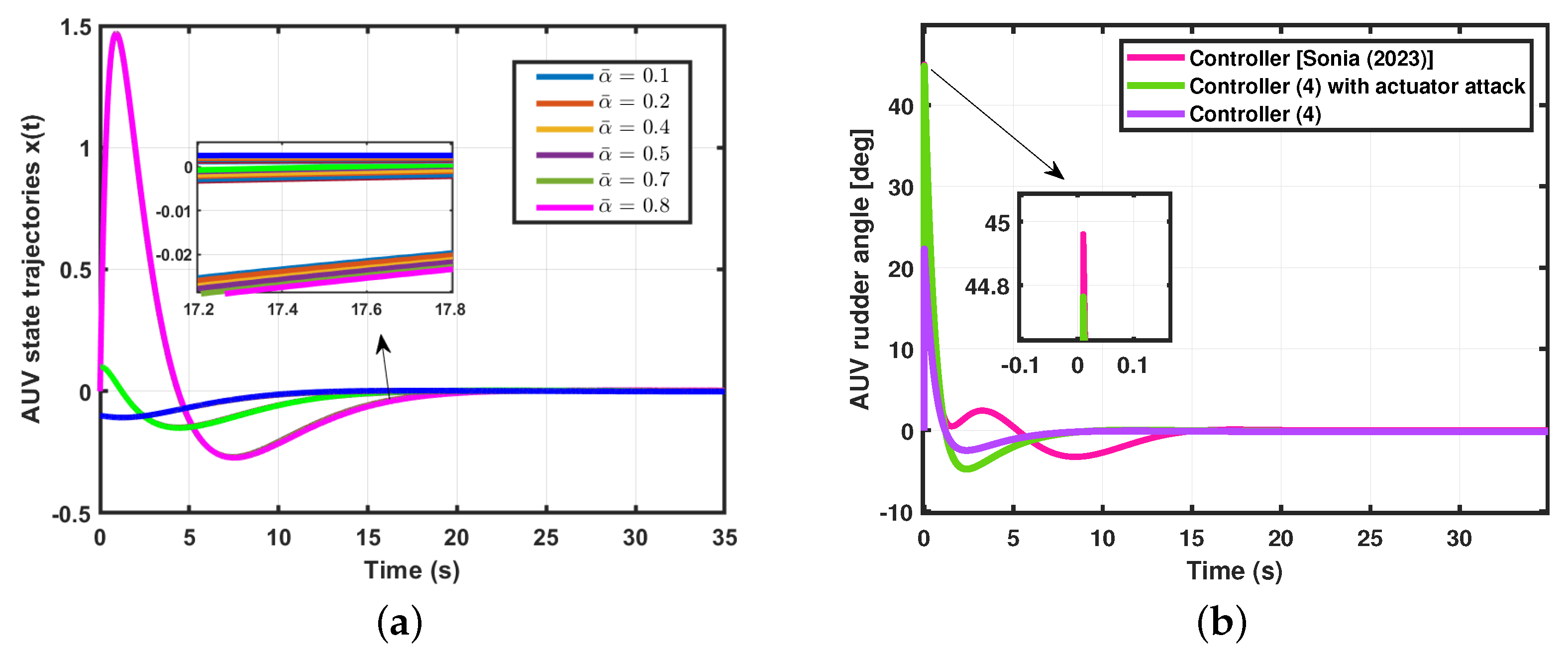
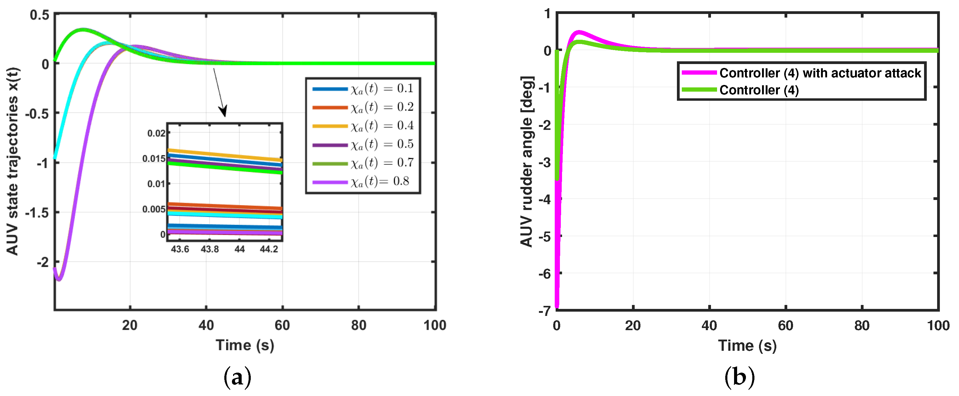
(AUV system I with time-varying delay) For the simulation of Theorem 1, using the following parameter values: time $t=0.01s$, $H_{\infty }$ performance level minimum $\gamma =0.02$, lower bound ${\tau }_m=0.01$, upper bound ${\tau }_M=1.96$, $\delta ={\tau }_M-{\tau }_m$, the probability of an random event occurs $\overline{\alpha }=0.7$, the possibility of an actuator attack $\overline{\beta }=0.9$, the possibility of a sensor attack $\overline{\gamma }=0.01$, the probability of an actuator attack ${\overline{\chi }}_a=0.2$, the probability of a sensor attack ${\overline{\chi }}_s=0.2$, $\mu =0.1$, $\rho =3.1$, and $\kappa =0.1$. We obtained the control gain matrix $K=[80.3706-142.5412-11.4617]$ for the AUV system (4). Thus, the state trajectories simulation result is shown in Figure 2.

Case 2.

(Randomly occurring uncertainties) When uncertainty occurring randomly occur with $\overline{\alpha }=0.1,0.2,0.4,0.5,0.7,0.8$ in system (4), the simulation results of these randomly occurring uncertainties are shown in Figure 3a.

Case 3.

(Actuator attack and controller comparison) The performance of controller (2), compared with previous work [19], is presented in Figure 3b. Moreover, the comparison of the controller with an actuator attack is shown in Figure 3b.

Case 4.

(Sensor attack and measured output) The simulation comparison of the measured output $y\left(t\right)$ with a sensor attack is shown in Figure 4a. Additionally, the disturbance graph is presented in Figure 4b.

A comparative analysis of the surge and sway positions, as well as the yaw angle, is presented in

Table 2. Comparative analysis of surge, sway positions, and yaw angle.

Settling Time(s)
Method	Surge	Sway	Yaw	Figure
Theorem 1	14.23	9.84	19.68	Figure 2
Sonia’s Method	20	19	22	Figure 8 in [19]

.

In

Table 3. Comparative analysis of controller (2) with [19].

Method	Lower Bound	Upper Bound	Controller Settling Time(s)
Theorem 1 (Figure 4b)	0.01	1.96	8.2
Controller (43) in [19]	0.01	1.8	14.97
Controller (60) in [19]	0.01	1.8	14.97

, the lower bound, upper bound, and controller settling time are compared with reference [19].

Case 5.

(Auxiliary state dynamics system I) For the simulation of Theorem 3, the AUV model in [19] uses the reference model matrices $A_r$, $C_r$, as defined in Table 1, and we use $G=[0.8002$$0.1480;$$0.01000.4000;0.4053-2.0530]$. The initial state of the reference model is $x_r\left(0\right)=[0.5\mathrm{m};0\mathrm{m}]$, which represents the surge and sway initial positions.

Moreover, Theorem 3 obtained the control gain matrix $K=[53.9297$$-64.1506-10.4171]$ by using the same parameters as Theorem 1. The surge and sway positions, as well as the yaw angle of the auxiliary system state trajectories, are shown in Figure 5.

 Example 2. 

We will adopt the continuous-time system as the one considered in [20], and the system matrices $A,B,C,A_r,$ and $C_r$ are defined in Example 1, and uncertain measurements $M_1=M_2=\left[\begin{array}{cc}0& 0\\ 0& 0\\ 0.00865& 0.00692\end{array}\right],N_1=N_2=\left[\begin{array}{ccc}1& 0& 0.4\\ 0& 1& 0\end{array}\right],$ $\Delta \left(t\right)=\left[\begin{array}{cc}sin\left(2\pi T_s\right)& 0\\ 0& sin\left(2\pi T_s\right)\end{array}\right]$. The initial states are $x\left(0\right)={[-1\mathrm{m}0\mathrm{m}-2^{\circ }]}^{\mathrm{T}}$, and time-varying delay is defined as $\tau \left(t\right)=0.98+0.95sin\left(t\right)$.

The first three cases present the simulation results for Theorem 2, and the last case presents the simulation results for Theorem 4.

Case 1.

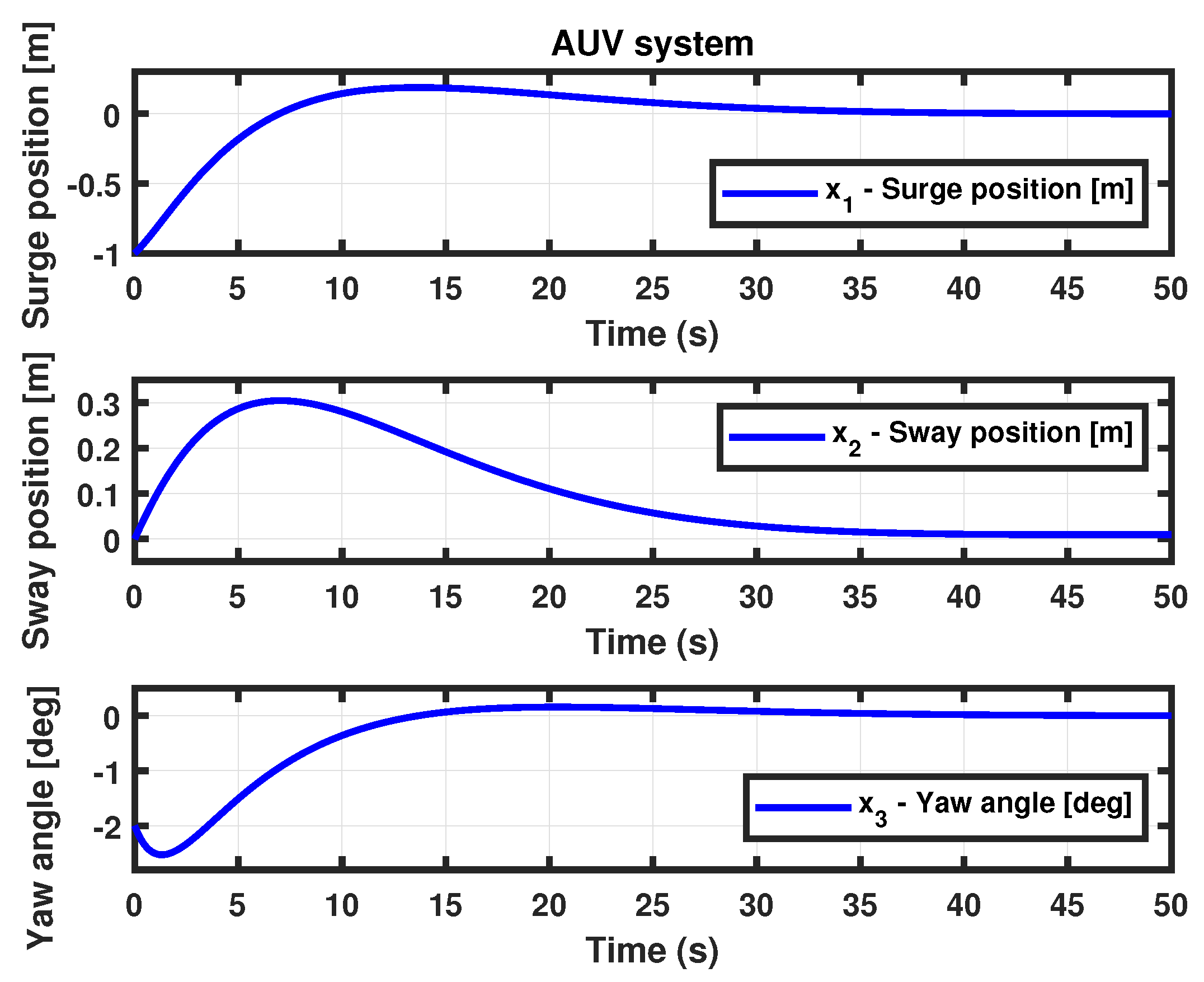
(AUV system II with time-varying delays) For the simulation of Theorem 2, we used the following parameter values: time $T_s=0.01s$, $H_{\infty }$ performance level minimum $\gamma =0.005$, lower bound ${\tau }_m=0.01$, upper bound ${\tau }_M=2.1$, $\delta ={\tau }_M-{\tau }_m$, the probability of an random event occurs $\overline{\alpha }=0.7$, the possibility of an actuator attack $\overline{\beta }=0.9$, the possibility of a sensor attack $\overline{\gamma }=0.1$, the probability of an actuator attack ${\overline{\chi }}_a=0.2$, the probability of a sensor attack ${\overline{\chi }}_s=0.2$, $\mu =0.1$, $\rho =2.8$, and $\kappa =0.1$. We obtained the controller gain matrix $K=[6.6535-6.1005-2.1372]$ for the AUV system (6). Thus, the state trajectories simulation result is presented in Figure 6.

Case 2.

(Actuator attacks and controller) When actuator attacks occur with ${\overline{\chi }}_a=0.1,0.2,$$0.4,0.5,0.7,0.8$ in system (6), the simulation results of these different probabilities of actuator attacks are shown in Figure 7a. The performance of the controller $u\left(t\right)$, compared with that of the actuator attack, is presented in Figure 7b.

Case 3.

(Sensor attacks and measured output) The simulation comparison of the measured output $y\left(t\right)$ with a sensor attack is shown in Figure 8a. Additionally, the time-varying delay $\tau \left(t\right)$ graph is presented in Figure 8b.

Case 4.

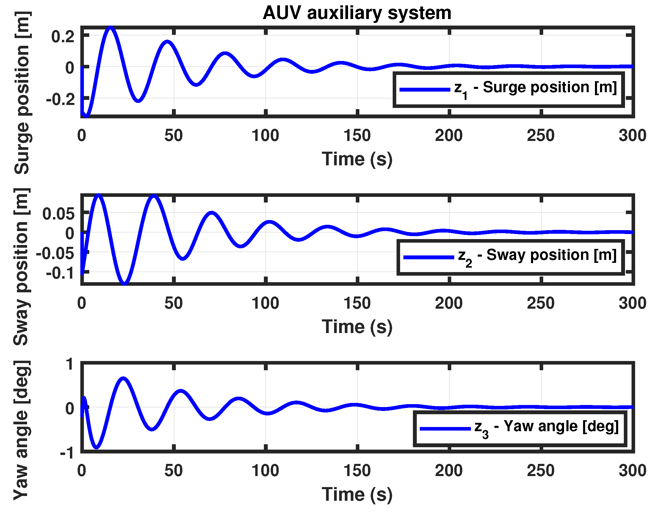
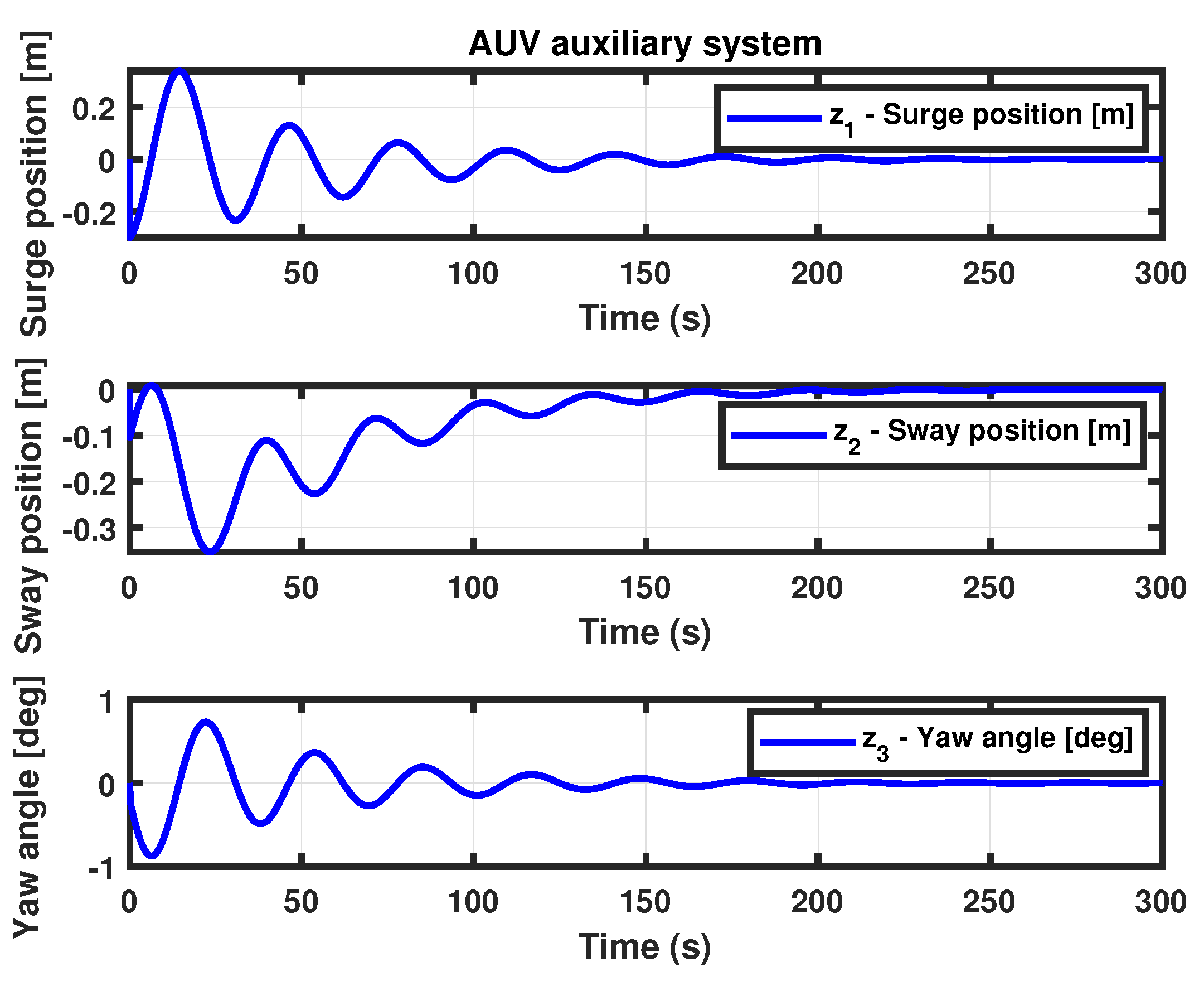
(Auxiliary state dynamics system II) Theorem 4 for the AUV auxiliary system yields the controller gain matrix $K=[5.0621-5.2353-1.7397]$, using the same parameter values as in Theorem 2. The surge and sway positions, along with the yaw angle of the auxiliary system state trajectories, are shown in Figure 9.

In

Table 4. Comparative analysis of surge, sway, and yaw positions.

Settling Time(s)
Method	Surge	Sway	Yaw	Figure
Theorem 4	200	190	210	Figure 9
Yu and Gao’s Method	1300	1250	1100	Figure 6 in [20]

, the surge, sway, and yaw positions are compared with those in reference [20].

5. Conclusions

In this article, we address the robust $H_{\infty }$ control problem of AUVs under time-varying delay, model uncertainties, and cyber-attacks. To the best of our knowledge, this paper is novel in addressing robust $H_{\infty }$ control, considering time-varying delays, cyber-attacks, and randomly occurring uncertainties in AUV systems.

A continuous-time linear uncertain time-varying delay system is established for the concerned AUVs. Based on the continuous-time time-varying delay system with consideration of randomly occurring uncertainties, a stochastic sensor and actuator attacks are derived. A robust $H_{\infty }$ controller is proposed for the established AUV systems under time-varying delay, uncertain random models, and cyber-attacks. It is proven that the resulting closed-loop system is asymptotically stable. In addition, asymptotic stability is discussed in the auxiliary state dynamic system.

Finally, the effectiveness of the proposed controller is verified through two computer simulation examples. Using computer simulations, we compare the performance of our robust $H_{\infty }$ control with the controls in [19,20], and demonstrate the outperformance of the proposed $H_{\infty }$ control.

References

1. Thuyen, N.A.; Thanh, P.N.N.; Anh, H.P.H. Adaptive finite-time leader-follower formation control for multiple AUVs regarding uncertain dynamics and disturbances. Ocean Eng. 2023, 269, 113503. [Google Scholar] [CrossRef]
2. Li, Y.; He, J.; Shen, H.; Zhang, W.; Li, Y. Adaptive practical prescribed-time fault-tolerant control for autonomous underwater vehicles trajectory tracking. Ocean Eng. 2023, 277, 114263. [Google Scholar] [CrossRef]
3. Wang, Y.; Wang, Z.; Chen, M.; Kong, L. Predefined-time sliding mode formation control for multiple autonomous underwater vehicles with uncertainties. Chaos Solitons Fractals 2021, 144, 110680. [Google Scholar] [CrossRef]
4. Li, J.; Du, J.; Chang, W.J. Robust time-varying formation control for underactuated autonomous underwater vehicles with disturbances under input saturation. Ocean Eng. 2019, 179, 180–188. [Google Scholar] [CrossRef]
5. Li, J.; Du, J.; Hu, X. Robust for dynamic positioning of ships under unknown disturbances and input constraints. Ocean Eng. 2020, 206, 107254. [Google Scholar] [CrossRef]
6. Li, X.G.; Wang, J.M. Fuzzy active disturbance rejection control design for autonomous underwater vehicle manipulators system. Adv. Control Appl. 2021, 3, e44. [Google Scholar] [CrossRef]
7. Liu, H.; Lyu, Y.; Lewis, F.L.; Wan, Y. Robust time-varying formation control for multiple underwater vehicles subject to nonlinearities and uncertainties. Int. J. Robust Nonlinear Control 2019, 29, 2712–2724. [Google Scholar] [CrossRef]
8. Xu, Y.; Wan, L.; Zhang, Z.; Chen, G. Robust adaptive path following control of autonomous underwater vehicle with uncertainties and communication bandwidth limitation. Ocean Eng. 2023, 287, 115895. [Google Scholar] [CrossRef]
9. Shojaei, K.; Chatraei, A. Robust platoon control of underactuated autonomous underwater vehicles subjected to nonlinearities, uncertainties and range and angle constraints. Appl. Ocean Res. 2021, 110, 102594. [Google Scholar] [CrossRef]
10. Li, T.; Wang, W.; Chen, W. Mixed H and passive event-triggered control for Markovian jump systems with sensor saturation under cyber-attacks. Asian J. Control 2022, 24, 3588–3600. [Google Scholar] [CrossRef]
11. Zhang, H.; Chen, Z.; Zhao, N.; Xing, B.; Mathiyalagan, K. Adaptive neural dissipative control for markovian jump cyber-Physical systems against sensor and actuator attacks. J. Frank. Inst. 2023, 360, 7676–7698. [Google Scholar] [CrossRef]
12. Nateghi, S.; Shtessel, Y.; Edwards, C. Resilient control of cyber-physical systems under sensor and actuator attacks driven by adaptive sliding mode observer. Int. J. Robust Nonlinear Control 2021, 31, 7425–7443. [Google Scholar] [CrossRef]
13. Syfert, M.; Ordys, A.; Kościelny, J.M.; Wnuk, P.; Możaryn, J.; Kukiełka, K. Integrated approach to diagnostics of failures and cyber-attacks in industrial control systems. Energies 2022, 15, 6212. [Google Scholar] [CrossRef]
14. Huang, X.; Dong, J. Secure tracking control against sensor and actuator attacks: A robust model-reference adaptive control method. Inf. Sci. 2022, 604, 11–27. [Google Scholar] [CrossRef]
15. Huang, X.; Xing, M.; Mo, H.; Hu, S.; Luo, H. Stabilization of uncertain networked control systems with actuator saturation and probabilistic cyberattacks. Asian J. Control 2023, 25, 1407–1419. [Google Scholar] [CrossRef]
16. Saravanakumar, T.; Lee, T. Hybrid-driven-based resilient control for networked T-S fuzzy systems with time-delay and cyber-attacks. Int. J. Robust Nonlinear Control 2023, 33, 7869–7891. [Google Scholar] [CrossRef]
17. Saravanakumar, T.; Nirmala, V.; Raja, R.; Cao, J.; Lu, G. Finite-time reliable dissipative control of neutral-type switched artificial neural networks with non-linear fault inputs and randomly occurring uncertainties. Asian J. Control 2020, 22, 2487–2499. [Google Scholar] [CrossRef]
18. Vimal Kumar, S.; Marshal Anthoni, S.; Raja, R. Dissipative analysis for aircraft flight control systems with randomly occurring uncertainties via non-fragile sampled-data control. Math. Comput. Simul. 2019, 155, 217–226. [Google Scholar] [CrossRef]
19. Ghrab, S.; Ahmed Ali, S.; Benamor, A.; Langlois, N.; Messaoud, H. A novel robust discrete-time integral sliding mode tracking control design for time-varying delay MIMO systems with unknown uncertainties. ISA Trans. 2024, 145, 1–18. [Google Scholar] [CrossRef]
20. Ghrab, S.; Benamor, A.; Messaoud, H. A new robust discrete-time sliding mode control design for systems with time-varying delays on state and input and unknown unmatched parameter uncertainties. Math. Comput. Simul. 2021, 190, 921–945. [Google Scholar] [CrossRef]
21. Hernández-González, O.; Ramírez-Rasgado, F.; Farza, M.; Guerrero-Sánchez, M.-E.; Astorga-Zaragoza, C.-M.; M’Saad, M.; Valencia-Palomo, G. Observer for Nonlinear Systems with Time-Varying Delays: Application to a Two-Degrees-of-Freedom Helicopter. Aerospace 2024, 11, 206. [Google Scholar] [CrossRef]
22. Campos-Martínez, S.-N.; Hernández-González, O.; Guerrero-Sánchez, M.-E.; Valencia-Palomo, G.; Targui, B.; López-Estrada, F.-R. Consensus Tracking Control of Multiple Unmanned Aerial Vehicles Subject to Distinct Unknown Delays. Machines 2024, 12, 337. [Google Scholar] [CrossRef]
23. Hernández-González, O.; Targui, B.; Valencia-Palomo, G.; Guerrero-Sánchez, M.-E. Robust cascade observer for a disturbance unmanned aerial vehicle carrying a load under multiple time-varying delays and uncertainties. Int. J. Syst. Sci. 2024, 55, 1056–1072. [Google Scholar] [CrossRef]
24. Li, Y.; Voos, H. An application of linear algebra theory in networked control systems: Stochastic cyber-attacks detection approach. IMA J. Math. Control Inf. 2015, 1–22. [Google Scholar] [CrossRef]
25. Li, Y.; Voos, H.; Rosich, A.; Darouach, M. A Stochastic Cyber-Attack Detection Scheme for Stochastic Control Systems Based on Frequency-Domain Transformation Technique. In Network and System Security. In Proceedings of the 8th International Conference, NSS 2014, Xi’an, China, 15–17 October 2014; Au, M.H., Carminati, B., Kuo, C.-C.J., Eds.; Springer: Cham, Switzerland, 2014; Volume 8792, pp. 209–222. [Google Scholar]
26. Zhang, X.; Xu, X.; Li, J.; Luo, Y.; Wang, G.; Brunauer, G.; Dustdar, S. Observer-based H fuzzy fault-tolerant switching control for ship course tracking with steering machine fault detection. ISA Trans. 2023, 140, 32–45. [Google Scholar] [CrossRef] [PubMed]
27. Lien, C.H.; Yu, K.W.; Wu, L.C.; Chung, L.Y.; Chen, J.D. Robust H1 switching control and switching signal design for uncertain discrete switched systems with interval time-varying delay. J. Frank. Inst. 2014, 351, 565–578. [Google Scholar] [CrossRef]
28. Wu, W.; Wang, X.; Rao, H.; Zhou, B. Delay-dependent Wide-area Damping Controller Synthesis Approach Using Jensen’s Inequality and Evolution Algorithm. CSEE J. Power Energy Syst. 2023, 9, 1774–17785. [Google Scholar]
29. Park, P.; Ko, J.W.; Jeong, C. Reciprocally convex approach to stability of systems with time-varying delays. Automatica 2011, 47, 235–238. [Google Scholar] [CrossRef]
Figure 1. Schematic diagram of AUV system in the presence of cyber-attacks and external disturbances.
Applsci 14 08827 g001
Figure 2. State trajectories of AUV for Theorem 1.
Applsci 14 08827 g002
Figure 3. Simulation results for Theorem 1. (a) Comparison of randomly occurring uncertainties α ¯ . (b) Controller (2) compared with actuator attack and [19].
Applsci 14 08827 g003
Figure 4. Simulation results for Theorem 1. (a) Comparison of output y(t). (b) Disturbance.
Applsci 14 08827 g004
Figure 5. Simulation results for Theorem 3.
Applsci 14 08827 g005
Figure 6. State trajectories of AUV for Theorem 2.
Applsci 14 08827 g006
Figure 7. Simulation results for Theorem 2. (a) Comparison of actuator attack χ a ( t ) . (b) Comparison of controller (2).
Applsci 14 08827 g007
Figure 8. Simulation results for Theorem 2. (a) Comparison of output y(t). (b) Time-varying delay τ ( t ) .
Applsci 14 08827 g008
Figure 9. Simulation results for Theorem 4.
Applsci 14 08827 g009