Scheduling Method of Demand-Responsive Transit Based on Reservation Considering Vehicle Size and Mileage

Abstract

Demand-responsive transit (DRT) is a kind of new public transit tailored to passenger needs that can provide passengers with fast, convenient, and diversified travel services. This paper proposes a scheduling model for demand-responsive transit based on reservations applicable to multi-vehicle task dispatching during the time period. It uses an ant colony algorithm for a solution. The model uses vehicle size and mileage as the optimization objectives while considering practical constraints like multi-vehicle operation, maximum pick-up intervals, etc. The feasibility of the model and the algorithm’s effectiveness are verified using the Shanghai Huyi Highway Demonstration Line as a case study. The results indicate that the model can effectively generate the optimal scheduling plan for DRT, significantly reduce the system’s operating cost, and improve resource utilization efficiency.

1. Introduction

Giving priority to the development of public transport is an indispensable way to enhance resource utilization and promote sustainable transport development. However, current conventional buses are seriously uncompetitive due to various problems such as overcrowded carriages, long waiting times for passengers, and low levels of traveling comfort.

To solve the above problems, demand-responsive transit (DRT) has emerged. DRT is a mode of public transportation to pick up and drop off passengers according to their travel requests at specific locations and does not have fixed routes and stops. It is flexible in terms of arrival time and operating routes and can help to improve the competitiveness of public transport, ease urban traffic congestion, and reduce traffic pollution. In the 1970s, Flusberg [1] first proposed the concept of DRT and successfully conducted it in a small city. The Transit Cooperative Research Program (TCRP) documents six types of DRT service: request stops, flexible route segments, route deviation, point deviation, zone routes, and demand-responsive connector service [2].

Entering the 21st century, the rapid development of emerging technologies such as artificial intelligence (AI) and big data provides a technological foundation for the realization of DRT. Therefore, how to efficiently and stably carry out the operation of DRT has become an urgent task in the study of urban public transport. Now, there has been a proliferation of research and practice on DRT. As an important part of the research on DRT, the DRT scheduling problem has achieved many results after years of development. The latest research progress is introduced from three aspects of optimization objectives, constraints, and solution algorithms as follows.

(1)

Optimization Objectives

Optimization objectives mainly include considering the costs of passengers and operators, energy consumption, and so on. Among them, the comprehensive consideration of the costs of passengers and operators is the mainstream research direction. Zheng et al. established a DRT scheduling equivalent decomposition model with minimum vehicle operating mileage and minimum use of vehicles as the objective function. They designed a distributed column generation algorithm to solve the problem [3]. Ghannadpour et al. researched the dynamic path optimization problem with a fuzzy time window, established a multi-objective model intending to minimize the operating cost, and used a genetic algorithm to solve the problem [4]. Narayan et al. combined demand-responsive buses with conventional buses and used the average waiting time of passengers as the optimization objective, and finally found that the average waiting time of users was lower than that of the two modes alone [5]. Shen et al. proposed a bus route optimization method based on the reliability of shortest paths to efficiently and quickly complete the passenger route optimization problem in a complex and changeable traffic environment. The method takes the minimization of total passenger and operating costs as the objective function and adopts the forbidden search algorithm to solve the problem [6]. Ding established a VRP model based on a single-vehicle DRT path optimization problem to minimize the total fleet operating time and the passenger service level reduced by early or delayed vehicle arrivals [7]. Sun et al. proposed a mixed integer linear model for DRT service that simultaneously minimizes the total mileage operating cost and maximizes passenger satisfaction [8]. Lu et al. considered both operator and passenger benefits to construct a multi-objective route optimization model with the minimum operating and passenger costs [9].

In the study considering minimum energy consumption, Li et al. embedded the eco-path strategy into the DRT service and integrated the vehicle dynamics module and the fuel consumption module for different traffic conditions and road types, which can significantly reduce energy consumption and emissions [10]. Ma et al. introduced the carbon emission objective in the route optimization model, which improves vehicle operating efficiency while reducing environmental costs [11].

(2)

Constraints

Existing studies have considered single or multiple constraints such as station, vehicle capacity, and time window constraints.

The station types include both fixed and variable stations. In the studies of fixed station constraints, Qiu et al. established a DRT scheduling model considering dynamic stations, the model in which the vehicle operation must pass through fixed stations, and passengers traveling on and off these fixed stations do not need to make reservations in advance. The model can reduce the number of car trips and reduce passenger costs at an unexpectedly high demand level [12]. Bruni et al. also researched DRT with fixed stations to introduce uncertainty into route scheduling to reduce vehicle detour costs [13]. Among the studies on variable station constraints, Petit et al. researched flexible DRT, in which passengers do not have to go to stations to obtain services, which can effectively reduce passenger costs [14,15]. Sun et al. constructed a flexible bus VRP scheduling model, solved it using a heuristic algorithm, and verified the effectiveness and robustness of the model and the algorithm with a case [16].

Vehicle capacity constraint is the limitation of an individual vehicle’s capacity on the scheduling method. In the study of vehicle capacity constraint, Wang et al. designed a high-degree-of-freedom responsive bus system and proposed an optimization method for vehicle routes, scheduling, and service areas, and constructed the model with vehicle capacity constraints [17]. Ren et al. considered two factors, capacity constraints and the time window, and transformed the problem into a joint optimization problem of fleet size allocation and vehicle routing with a full-service process time window and capacity constraints to solve it [18].

The time window is the duration from the earliest to the latest departure time that passengers can catch up with after making a reservation. Wang et al. introduced a passenger incentive preference policy to reduce the ineffective distance and time of the vehicle by incentivizing passengers to make passengers arrive at their designated locations on time [19]. Wang et al. investigated the DRT path optimization and vehicle scheduling problem with a time window, vehicle operation time, departure time, and other constraints, constructed an optimization model, and solved it by using a dual genetic algorithm [20]. Shen et al. added time window constraints and considered vehicle punctuality constraints, passenger travel deviation, and passenger real-time demands in the model, which can meet passenger travel demands and improve passenger travel satisfaction [21].

(3)

Solution Algorithm

The algorithms for solving the DRT scheduling problem include two categories: exact algorithms and heuristic algorithms. The exact algorithms refer to a class of algorithms that spend a limited amount of computation time to obtain the optimal optimization problem solution through precise mathematical and logical operations. The exact algorithms include branch-and-bound [22,23,24], cut-plane [25,26], and dynamic programming [27,28]. When the size of the problem is small, the exact algorithm can be solved effectively within an acceptable time. However, when the size and complexity of the solution increase, the computation time required will show an exponential growth trend.

Compared to exact algorithms, heuristic algorithms can achieve better results for more complex problems. Therefore, since the 1990s, many scholars have focused on researching the application of heuristic algorithms to solve vehicle scheduling problems. The commonly used heuristic algorithms include the tabu search algorithm (TSA), simulated annealing algorithm (SAA), ant colony optimization (ACO), genetic algorithm (GA), and so on. Bruni et al. proposed a new formulation of stochastic mixed-integer programming and described an effective TSA [13]. Nie studied the operational characteristics of DRT in-depth, established the DRT path optimization models for single and multiple access points, and used an improved TSA to find the optimal solution [29]. Jin et al. developed a customized SAA to introduce flexible quality of service into the DRT feeder transportation problem, which can reduce infeasible solutions and improve search efficiency [30]. Sun et al. selected a collaborative ACO to compute the DRT model with fuzzy demand, redefined pheromones, heuristic information, etc., and solved the limitations of the traditional ACO [31]. Jin et al. combined the advantages of the GA and the ACO and added the destination dimensionality reduction operator, which gave the algorithm a stronger solving ability and better stability [32]. He et al. designed an algorithm based on GA by constructing an optimization model that considered the operating costs and reliability of the DRT line design problem. The results showed that the new algorithm had obvious advantages regarding computational efficiency and performance [33]. Perera et al. improved the GA by increasing the number of iterations of the genetic operator and schedulable passengers to generate highly accurate schedules and reduce passengers’ travel time [34].

Existing studies have achieved rich research results and formed a relatively perfect theoretical system. However, the scheduling models in the literature have only considered the case of a single vehicle size. But due to the single limitation of vehicle size capacity, coupled with the complexity and variability of the roads, it is easy to lead to a mismatch between the number of passengers and vehicles in practice, resulting in a waste of resources, so it is necessary to consider the case of multiple vehicle sizes. Moreover, established research also did not consider the case of multiple vehicle yards or just set both departures and returns to enter the same yard to reduce the difficulty of solving. Still, the reality is often to take a multiple vehicle yard scheduling mode. Therefore, this paper establishes a DRT scheduling model suitable for multiple vehicle sizes and yards. The contributions of this study are summarized as follows:

(1)

A directed acyclic graph is used to describe the scenario of DRT based on the reservation scheduling problem;

(2)

The constraints integrate the practical limitations such as multiple vehicle sizes, maximum pick-up interval time, etc., and an ant colony algorithm is designed according to the characteristics of the model to solve the problem.

(3)

The model gets rid of the limitation of single vehicle yards, so the applicability of the model is wider, and it can be applied to multi-model vehicle scheduling in single and multiple vehicle yards.

2. Mathematical Modelling

2.1. Problem Description Based on Directed Acyclic Graph

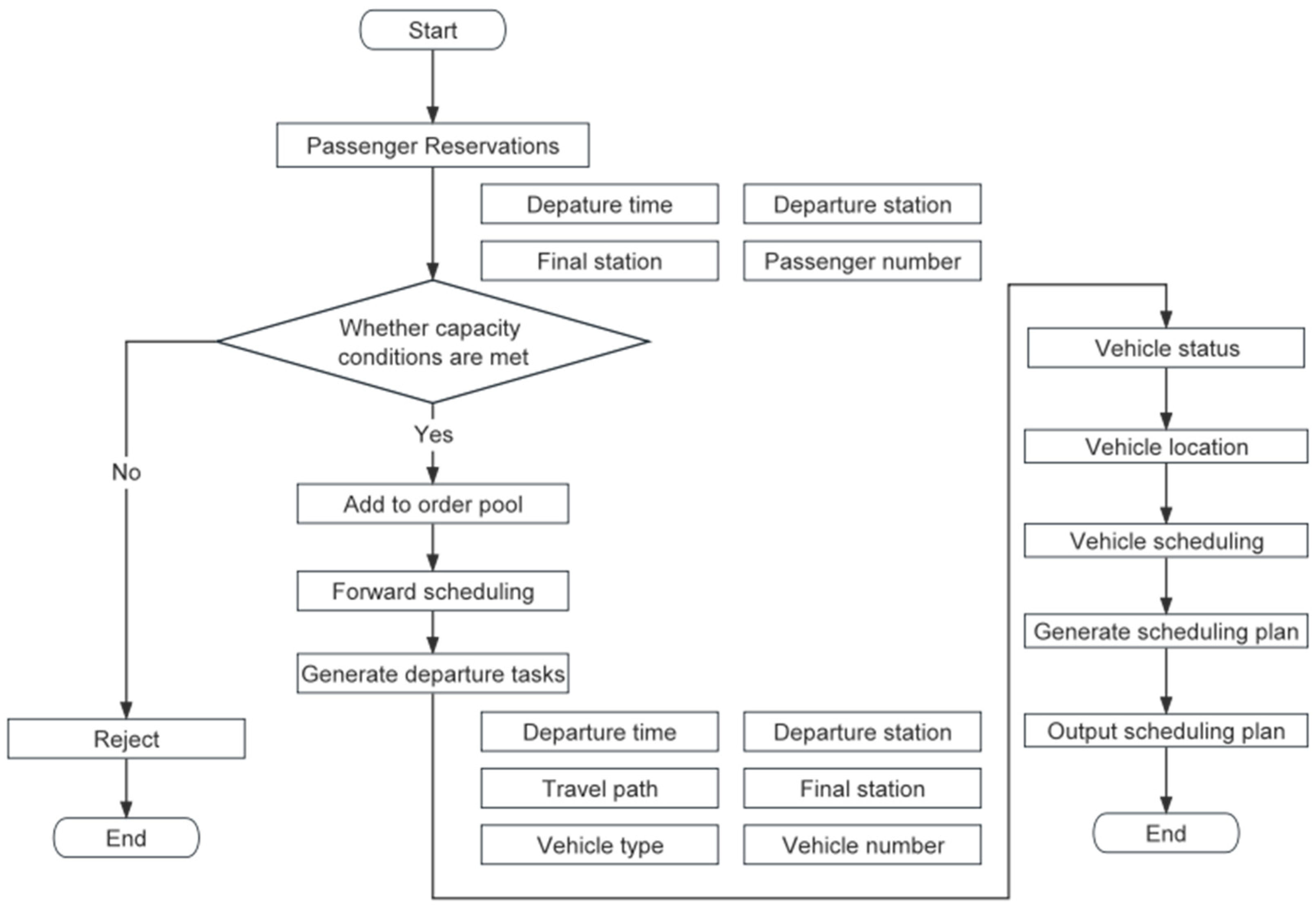
For DRT based on reservations, only the bus stations and available departure times are fixed. At the same time, passengers can choose the appropriate departure time, departure station, and final station according to their needs. A defined time point will stop reservations for a certain time period. The system will generate orders and vehicle scheduling plans based on this information. Figure 1 shows the reservation-based DRT scheduling process. After the passengers make a reservation, the system filters the orders that meet the service requirements based on the capacity conditions and adds them to the order pool. Once the reservation time closes, the pre-scheduling system generates all the departure tasks within that time period, including departure time, departure station, travel path, final station, vehicle size, and vehicle number. After the departure tasks are determined, each will be assigned to the corresponding vehicle before departure according to the vehicle location distribution status and availability provided by the big data center, which ultimately forms the overall vehicle scheduling plan.

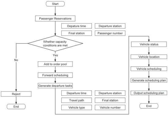
Figure 1. The reservation-based DRT scheduling process.

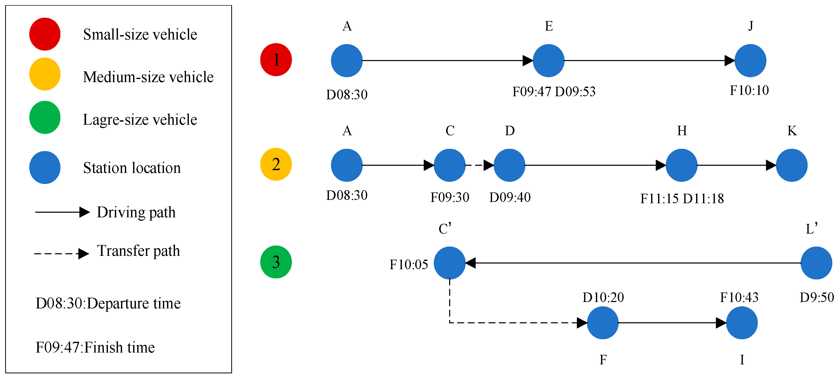
If two or more departure tasks require the same vehicle size and the departure and arrival times of the individual tasks, they do not conflict with each other. These departure tasks can be accomplished with a single vehicle. The number of vehicles required to complete all the tasks will be significantly reduced. Figure 2 shows a series of tasks during a time slot. There are 7 departure tasks in the figure, forming a total of 3 vehicle chains, which means that only 3 vehicles need to be called to complete the 7 vehicle tasks.

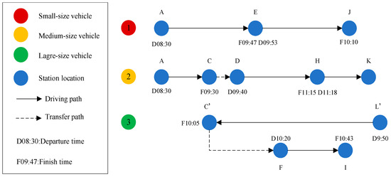
Figure 2. Diagram of a series of tasks during a time slot.

The above problem can be formulated as a network in terms of a directed acyclic graph. In graph theory, a directed graph is called a Directed Acyclic Graph (DAG) if it is impossible to return to any vertex in a directed graph by passing through several edges. Each departure task (including departure time, departure station, travel path, final station, and vehicle size) is abstracted as a node, and the conditions of time, space, and vehicle succession between departure tasks are transformed into the connecting edges between different nodes. Suppose two departure tasks can meet the conditions for articulated scheduling under certain constraints. In that case, they are said to be compatible and matchable, shown in Figure 3a, and they can be transformed into the form in Figure 3b. With minimum vehicle size as the single optimization objective, the vehicle scheduling problem can be transformed into a simple problem of finding the least disjoint coverage path in a DAR.

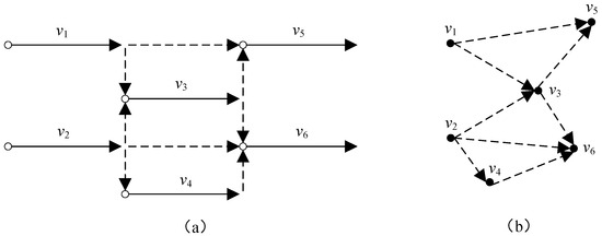
Figure 3. Representation of the vehicle scheduling problem in the form of DAG. (a) Representation of the vehicle scheduling problem. (b) The DAG after the transformation of scheduling problem.

2.2. Model Formulation

2.2.1. Basic Assumptions of the Model

To better abstract this problem into a mathematical model based on the actual situation, this paper makes the following assumptions:

(1)

The departure time, departure station, final station, and the required vehicle size for each departure task during the time period are determined and known;

(2)

Any basic information of any of the vehicles, including real-time passenger status of vehicles and so on, is known;

(3)

The locations of the yards and stations are known, and the driving distances between the stations are known;

(4)

To ensure the level of service, it is necessary to ensure an adequate number of vehicles of each size;

(5)

After the previous task has ended, the vehicle stays at the previous station and waits for dispatch.

(6)

During actual operation, vehicles are allowed to turn around.

(7)

Only a single trip for any vehicle during the time period.

(8)

When matching and connecting between departure tasks, certain scheduling time intervals or distance restrictions are required to prevent unrealistic vehicle scheduling in terms of time or distance.

(9)

The impact on vehicle scheduling due to unexpected events and other reasons is not considered.

2.2.2. Description of Model Parameters

Based on the above assumptions, if $L$ is the set of stations and $K$ is the set of vehicle sizes, for a certain period of time, according to the reservation data, all the vehicle tasks generated by the previous scheduling are sorted by departure time to form the set of departure tasks $M=\left\{M_k\left|k=\left(1,2,3\right)\right.\right\}=\left\{V_1,V_2,\cdots ,V_i,V_j,\cdots \right\}$, where $M_k$ represents the set of departure tasks with the required vehicle size $k$, $k=\left(1,2,3\right)$ represents small vehicles, medium vehicles, and large vehicles respectively, and $V_i$ and $V_j$ represent the vehicle tasks with the number $i$, $j$. For task $V_i$, there are $V_i=\left\{l_i^o,l_i^d,t_i^o,k_i\right\}$, where $l_i^o$ and $l_i^d$ represent the departure station and the final station of the task $V_i$, $t_i^o$ represents the departure time of the starting station of the training task, and $k_i$ represents the required vehicle size of the task $V_i$. After identifying the departure demand during the period, optimizing the matching and connection between the trips can determine the best vehicle scheduling plan.

The symbols and descriptions of the parameters used in the scheduling model are detailed in Glossary.

2.2.3. Objective Function

The target of vehicle scheduling is to arrange the most suitable vehicle for each departure task and form the most reasonable vehicle chain for each vehicle so that the system can operate efficiently and orderly with the lowest total operating cost. In a real-time scenario, vehicles need to be assigned in a coordinated manner because there are multiple departure time points in a time period, and the good or bad vehicle scheduling solution affects not only the length of vehicle mileage but also the size of vehicles. Therefore, the optimization objective of the model is determined as the total number of vehicles used and the total traveling mileage.

(1)

Vehicle number

The number of the system’s vehicles is determined by the number of tasks that need to be completed during the time period, and the vehicle scheduling scheme also influences it. If 2 tasks can be directionally matched to each other, they can be completed with the same vehicle, reducing the number of vehicles needed by 1. The more vehicles are matched between task points, the more the vehicle size is reduced, and the fewer vehicles are required. This leads to the formula for calculating the required vehicle size, as shown in Equation (1).

$$Z_1={\displaystyle \sum _{k\in K}(M_k-{\displaystyle \sum _{i,j\in M_k}{y}_{ij}})}$$

(1)

(2)

Traveling mileage

The total mileage during the time period includes two categories: fixed mileage and deadhead mileage. The fixed mileage refers to the vehicle mileage required between the departure station and final station of each task. The vehicle task is determined, so the fixed mileage is certain, and the reduction of the driving mileage only needs to consider the deadhead mileage. The formula for calculating the total deadhead mileage is shown in Equation (2).

$$Z_2={\displaystyle \sum _{k\in K}{\displaystyle \sum _{i,j\in M_k}{s}_{ij}{y}_{ij}}}$$

(2)

The model’s objective function is obtained by combining the two optimization objectives.

$$\min Z_p=Z_1^{\prime }+Z_2^{\prime }={\displaystyle \sum _{k\in K}(p_k(M_k-{\displaystyle \sum _{i,j\in M_k}{y}_{ij}})+q_k({\displaystyle \sum _{i,j\in M_k}{s}_{ij}{y}_{ij}}))}$$

(3)

2.2.4. Constraints

The constraints of the model are shown below.

$${\displaystyle \sum _{i\in M}{y}_{ij}\le 1}\forall j\in M$$

(4)

$${\displaystyle \sum _{j\in M}{y}_{ij}\le 1\forall i\in M}$$

(5)

$$(t_i^d+t_{ij})y_{ij}\le t_j^o\forall i,j\in M$$

(6)

$$(k_i-k_j)y_{ij}=0\forall i,j\in M$$

(7)

$$(t_j^o-t_i^d)y_{ij}\le \beta \forall i,j\in M$$

(8)

$$y_{ij}=\left\{\begin{array}{l}1i\mathrm{match}j\\ 0\mathrm{otherwise}\end{array}\right.$$

(9)

In the above constraints, Equation (4) means that every task can only be matched once by one vehicle or not. Equation (5) means that every vehicle can only match one task or not. Equations (6)–(8) are the necessary conditions for matching between two tasks. Equation (6) indicates that the time when the vehicle is transferred to the departure station of the next task after the previous task is finished must be earlier than the departure time of the next vehicle. Equation (7) indicates that the required vehicle sizes of the two tasks that can be matched must be the same. Since there is demand matching between different vehicle sizes, the case of larger-size vehicles replacing smaller-size vehicles is not considered. Equation (8) indicates that unrealistic matching scheduling of excessive time and distance is avoided. Equation (9) indicates that the decision variable $y_{ij}$ is a 0–1 variable. When $y_{ij}$ = 1, it means that vehicle task i matches vehicle task j, i.e., the vehicle executes vehicle task j after completing vehicle task i. When $y_{ij}$ = 0, vehicle task i does not match vehicle task j, i.e., the vehicle cannot execute vehicle task j after completing vehicle task i.

The station locations determine the distance parameter in the model, and the inter-station distance can be obtained by knowing the two station locations. Equations (10) and (11) show the calculation method of $s_i$ and $s_{ij}$.

$$s_i=F(l_i^o,l_i^d)$$

(10)

$$s_{ij}=F(l_i^d,l_j^o)$$

(11)

In addition, although the departure time of each task is determined, the actual travel time may be affected by many factors, so the vehicle’s arrival time needs to be predicted. Since the travel time prediction is not the focus of this paper, the travel time in this model is calculated by using the travel distance and the average running speed of the vehicle, i.e., so:

$$t_i^d=t_i^o+{\displaystyle \frac{s_i}{v}}$$

(12)

$$t_{ij}={\displaystyle \frac{s_{ij}}{v}}$$

(13)

3. Algorithm

The ant colony algorithm is a chance-based algorithm used to find optimized paths in a graph. Its thinking is inspired by the phenomenon that ant colonies in nature always find the shortest paths during their foraging process. In this paper, the ant colony algorithm is designed according to the model characteristics to solve the problem.

3.1. Feasible Path Construction

All the tasks are arranged in ascending order of departure time, and each ant can represent a different vehicle. At the initial moment, the ant is placed randomly on the earliest departure task point and then selects a task point as the next point of the path with a certain probability from $M_i^{k\_ant}$ that has not yet passed through and is allowed to match. When no more matching tasks can be found, i.e., $M_i^{k\_ant}=\varnothing$, the path construction is completed. Currently, the ant randomly selects a point as the initial point among the earliest departure task points that have not been experienced. The above steps are performed to build a new path again, and the cycle continues until all task points are traversed and a feasible path is built. The steps to generate the set of successive task points allowed by ants k at task i $M_i^{k\_ant}$ are as follows:

Step 1: Set $M_i^{k\_ant}=\varnothing$, no_visited as the set of task points to be visited.

Step 2: $\forall j\in no\_visited$, if Equations (5)–(7) hold simultaneously, then $M_i^{k\_ant}=M_i^{k\_ant}\cup \left\{j\right\}$, $no\_visited=no\_visited-\left\{j\right\}$, go to step 3.

Step 3: If $no\_visited\ne \varnothing$, go to step 2; else, go to step 4.

Step 4: Save the results of $M_i^{k\_ant}$ and terminate the loop.

3.2. Pheromone and Inspired Information Settings

The pheromone ${\tau }_{ij}$ represents the empirical information accumulated in the process of ant colony finding, which comes from the continuous exploration process of the ant colony. The inspired information ${\eta }_{ij}$ represents the influence of priori, deterministic factors in the process of finding. They will be directly related to the global convergence speed and solution efficiency of the ant colony algorithm.

The pheromone ${\tau }_{ij}$ indicates the expected degree of ants passing task point i and then passing task point j, and its value will be updated continuously as the ants seek the best. In the process of constructing a feasible solution to the vehicle scheduling problem, to lower the target cost, the shorter the matchable inter-task point idle distance $s_{ij}=F(l_i^d,l_j^o)$ is, the better. Therefore, the inspired information is taken as ${\eta }_{ij}=1/s_{ij}$, and when $s_{ij}=0$, ${\eta }_{ij}=1/(s_{ij}+0.1)$, where the significance of the constant term is to avoid the denominator being 0, which leads to anomalous heuristic information.

3.3. Selection Strategy

At the initial moment, the pheromone concentration of each path remains the same. The inspired information occupies the main influence in the path selection behavior of ants. Still, as time goes by, the pheromones on the path gradually accumulate, and the heuristic information and the pheromone content information work together to guide the ants in path selection. The ant k decides its transfer direction according to the pheromone and inspired information on each path during its movement. The state transfer probability of the ant k located at task point i choosing task point j as the matching succession point is expressed as $p_{ij}^{k\_ant}$, which is calculated as follows:

$$p_{ij}^{k\_ant}(t)=\left\{\begin{array}{c}{\displaystyle \frac{{\left[{\tau }_{ij}(t)\right]}^{\alpha }{\left[{\eta }_{ij}(t)\right]}^{\beta }}{{\displaystyle \sum _{j\in M_i^{k\_ant}}{\left[{\tau }_{ij}(t)\right]}^{\alpha }{\left[{\eta }_{ij}(t)\right]}^{\beta }}}},j\in M_i^{k\_ant}\\ 0,\mathrm{other}\end{array}\right.$$

(14)

$M_i^{k\_ant}$ is the set of allowed successive task points of ants k located at task point i; ${\tau }_{ij}(t)$ represents the pheromone content on the path $(i,j)$ at the moment of $t$; ${\eta }_{ij}(t)$ is the expected heuristic value of the path $(i,j)$ at the moment of $t$. $\alpha$ is the pheromone factor, which represents the relative importance of pheromone influence in the searching process of ants. The larger the value of $\alpha$, the more obvious the positive feedback effect is, but the randomness of the search is weakened. $\beta$ is the heuristic function factor, which represents the relative influence of expected heuristic information in the movement process of ants. The greater the value of $\beta$, the greater the likelihood that the ant will choose a locally optimal path at the task point. In this paper, to effectively reduce the randomness of ant state transfer and avoid the stagnation phenomenon, the pseudo-random ratio selection rule is chosen; that is, the deterministic selection and randomness selection are combined based on the original state transfer probability calculation shown in Equation (14), and the rule is shown in Equation (15).

$$j=\left\{\begin{array}{c}\arg \underset{j\in M_i^{k\_ant}}{\max }\left\{{\left[{\tau }_{ij}(t)\right]}^{\alpha }{\left[{\eta }_{ij}(t)\right]}^{\beta }\right\},r\le r_0\\ \left(4.14\right),r>r_0\end{array}\right.$$

(15)

$r$ is a random variable on the interval [0, 1]. $r_0$ is a parameter used to control the transfer rule, $0\le r_0\le 1$. When $r\le r_0$, the ant directly chooses the next succession task point. When $r>r_0$, ants calculate the state transfer probability at each point by Equation (14) and apply the roulette wheel method to determine the next succession task point.

3.4. Pheromone Update Rules

The global information update is used after the ants complete a single cycle for the ants that achieve the optimal solution in each generation of search, and the global information update rule is calculated as shown below.

$${\tau }_{ij}(t+1)=(1-\rho )\cdot {\tau }_{ij}(t)+{\displaystyle \frac{Q}{f_b}}$$

(16)

Among them, $\rho$ is the pheromone volatility factor, which reflects the volatility speed of pheromones and is located in the interval of $(0,1)$. When $\rho$ is too large, the pheromone volatility is too fast, the search randomness is weak, and it is easy to fall into the local optimum. When it is too small, the search randomness is enhanced, but the difference in the pheromone content of each path is reduced, and the convergence is too slow. $f_b$ do ants obtain the optimal objective function value in the current iteration. $Q$ is the pheromone constant, representing the total amount of pheromone released by ants in one cycle. When $Q$ is too large, it tends to accumulate pheromones rapidly and reduce the search range of the ant colony, leading to premature convergence and the local optimum. It tends to fall into a chaotic state when it is too small.

3.5. Algorithm Solving Steps

Figure 4 shows the flow chart of the ant colony algorithm for solving the scheduling model.

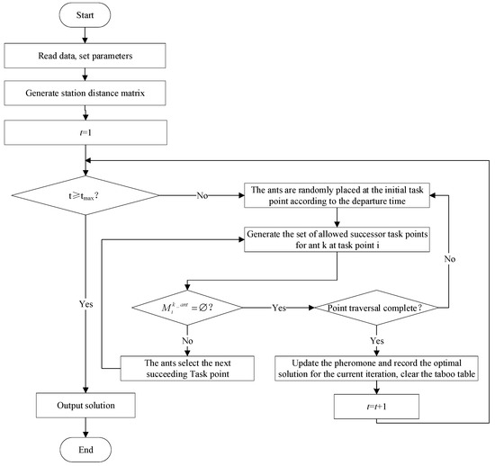
Figure 4. Flow chart of the ant colony algorithm.

The specific process of the optimization algorithm is as follows:

Step 1: Start. Read the departure task data and set the values of the parameters, including the average speed, the fixed costs, the deadhead cost per unit distance, and the maximum succession interval.

Step 2: Initialization of ant colony algorithm parameters, including the number of ants $m$, the pheromone factor $\alpha$, the heuristic function factor $\beta$, the pheromone volatility factor $\rho$, the pheromone constant $Q$, and the maximum number of iterations $t_{\max }$.

Step 3: Generate the site distance matrix. Generate the inter-site distance matrix according to the actual location of each site for heuristic function value calculation.

Step 4: Determine whether the current ant colony iteration number $t$ is greater than $t_{\max }$. If the judgment result is yes, the algorithm ends, and the current ant path solution set is output; otherwise, go to step 5.

Step 5: Randomly place the ants at the initial task point according to the task departure time.

Step 6: Generate the set of allowed succession task points $M_i^{k\_ant}$ of ants $k$ in task $i$, and judge whether $M_i^{k\_ant}$ is empty. If the judgment result is yes, go to step 8; otherwise, go to step 7.

Step 7: The ant selects the next successive task point according to the selection strategy and returns to step 6.

Step 8: Judge whether the task point traversal is completed. If the judgment result is yes, go to step 9; else, return to step 5.

Step 9: Update the pheromone. Update the pheromone concentration on each path, record the optimal solution for the current iteration $t=t+1$, empty the taboo table, and return to step 4.

4. Case Study

4.1. Data Description

The demonstration line of Huyi Highway (Chenxiang Road–Yecheng Road) is 8.2 km long and adopts a point-to-point direct operation mode for the whole line. Passengers initiate online demand reservations from the APP and select the departure time and the departure and finish stations. After unified collation, the passenger service system sends the reservation information to the backend scheduling system. The scheduling system generates the departure plan and driving route according to the demand data and dispatches the corresponding vehicles to complete the transportation task on time.

There are 12 custom bus stops on the line. The distance between each station is obtained using the information displayed on the electronic map. Take Zhaoxian Road as the first station, and the distance between each station and the first station is shown in Table 1.

Table 1. Distance between stations on the demonstration line of Huyi Highway.

Station Number	Station Name	Distances
01	Zhaoxian Road, Huyi Highway	0
02	Hongde Road, Huyi Highway	587
03	Baiyin Road, Huyi Highway	1117
04	Shigang	1683
05	Yining Road, Huyi Highway	2215
06	Huyi Highway Hope Road	2696
07	Huyi Highway Double Single Road	3336
08	Malu Town	3896
09	Huyi Highway Bao’an Highway	4540
10	Yagang Road, Huyi Highway	5393
11	Da Qiaotou	7093
12	Huyi Highway Chenxiang Road	7745

The average traveling speed of the demonstration line bus is 60 km/h. Line operation temporarily uses three models. After reviewing relevant information and combining it with the actual situation, considering the vehicle depreciation, the cost of each model is set in Table 2.

Table 2. The basic information of the vehicles on the demonstration line of Huyi Highway.

Vehicle	Seating Capacity	Vehicle Size	Fixed Cost	Operating Cost	Deadhead Traveling Cost
2020SAIC Roewe Ei5 (Shanghai, China)	5 seats	Small	36 CNY/km	1.35 CNY/km	1.30 CNY/km
2021Maxus EV90 (Shanghai, China)	15 seats	Medium	40 CNY/km	1.90 CNY/km	1.85 CNY/km
Yancheng Brand HYK6700YBEV (Hengyang, China)	23 seats	Large	55 CNY/km	2.10 CNY/km	2.05 CNY/km

Considering the situation of the demonstration line, the deployable time point is set at 10 min intervals between 7:00 and 9:00, and the maximum succession interval is set at 30 min. During the two hours, 180 tasks are randomly generated, and some are shown in Table 3.

Table 3. Part of the departure tasks information.

Task Number	Departure Station	Final Station	Vehicle Size	Departure Time
1	Yining Road, Huyi Highway	Huyi Highway Double Single Road	Small	7:20
2	Hongde Road, Huyi Highway	Huyi Highway Double Single Road	Medium	8:50
3	Hongde Road, Huyi Highway	Huyi Highway Hope Road	Small	8:30
4	Huyi Highway Bao’an Highway	Huyi Highway Hope Road	Medium	8:10
5	Malu Township	Huyi Highway Hope Road	Medium	8:50
6	Hongde Road, Huyi Highway	Malu Township	Large	7:50
7	Baiyin Road, Huyi Highway	Da Qiaotou	Small	8:00
8	Huyi Highway Bao’an Highway	Huyi Highway Double Single Road	Small	7:00
9	Yagang Road, Huyi Highway	Shigang	Medium	8:40
10	Zhaoxian Road, Huyi Highway	Huyi Highway Double Single Road	Medium	7:10
11	Baiyin Road, Huyi Highway	Hongde Road, Huyi Highway	Medium	7:00
12	Huyi Highway Hope Road	Zhaoxian Road, Huyi Highway	Small	7:40
13	Baiyin Road, Huyi Highway	Yagang Road, Huyi Highway	Large	8:10
14	Yagang Road, Huyi Highway	Huyi Highway Bao’an Highway	Large	7:50
15	Malu Township	Baiyin Road, Huyi Highway	Large	8:40
16	Huyi Highway Double Single Road	Huyi Highway Chenxiang Road	Medium	9:00
17	Hongde Road, Huyi Highway	Huyi Highway Chenxiang Road	Small	7:20
18	Da Qiaotou	Huyi Highway Bao’an Highway	Large	8:40
19	Da Qiaotou	Zhaoxian Road, Huyi Highway	Small	8:50
20	Huyi Highway Bao’an Highway	Baiyin Road, Huyi Highway	Small	7:40
21	Yagang Road, Huyi Highway	Baiyin Road, Huyi Highway	Large	8:20
22	Huyi Highway Chenxiang Road	Huyi Highway Hope Road	Small	8:30
23	Yagang Road, Huyi Highway	Huyi Highway Hope Road	Small	7:50
24	Huyi Highway Double Single Road	Baiyin Road, Huyi Highway	Medium	8:10
25	Huyi Highway Chenxiang Road	Huyi Highway Hope Road	Large	8:10
26	Hongde Road, Huyi Highway	Baiyin Road, Huyi Highway	Medium	8:30
27	Da Qiaotou	Baiyin Road, Huyi Highway	Medium	7:10
28	Da Qiaotou	Shigang	Small	8:30
29	Hongde Road, Huyi Highway	Huyi Highway Bao’an Highway	Small	8:10
30	Huyi Highway Bao’an Highway	Hongde Road, Huyi Highway	Medium	7:00
……	……	……	……	……

Table 4 sets the values of each parameter of the ant colony algorithm, based on previous research experience and the actual situation of the line.

Table 4. Values of the parameters of the ant colony algorithm.

Parameter	Explanation	Value
m	Total number of ant colonies	30
tmax	Iteration number	200
Q	Total number of pheromones	200
τ0	Initial value of pheromone	1
$\rho$	Pheromone volatility factor	0.3
r0	Roulette impact factor	0.5
α	Pheromone impact factor	1
β	Inspired function impact factor	3

4.2. Analysis of Results

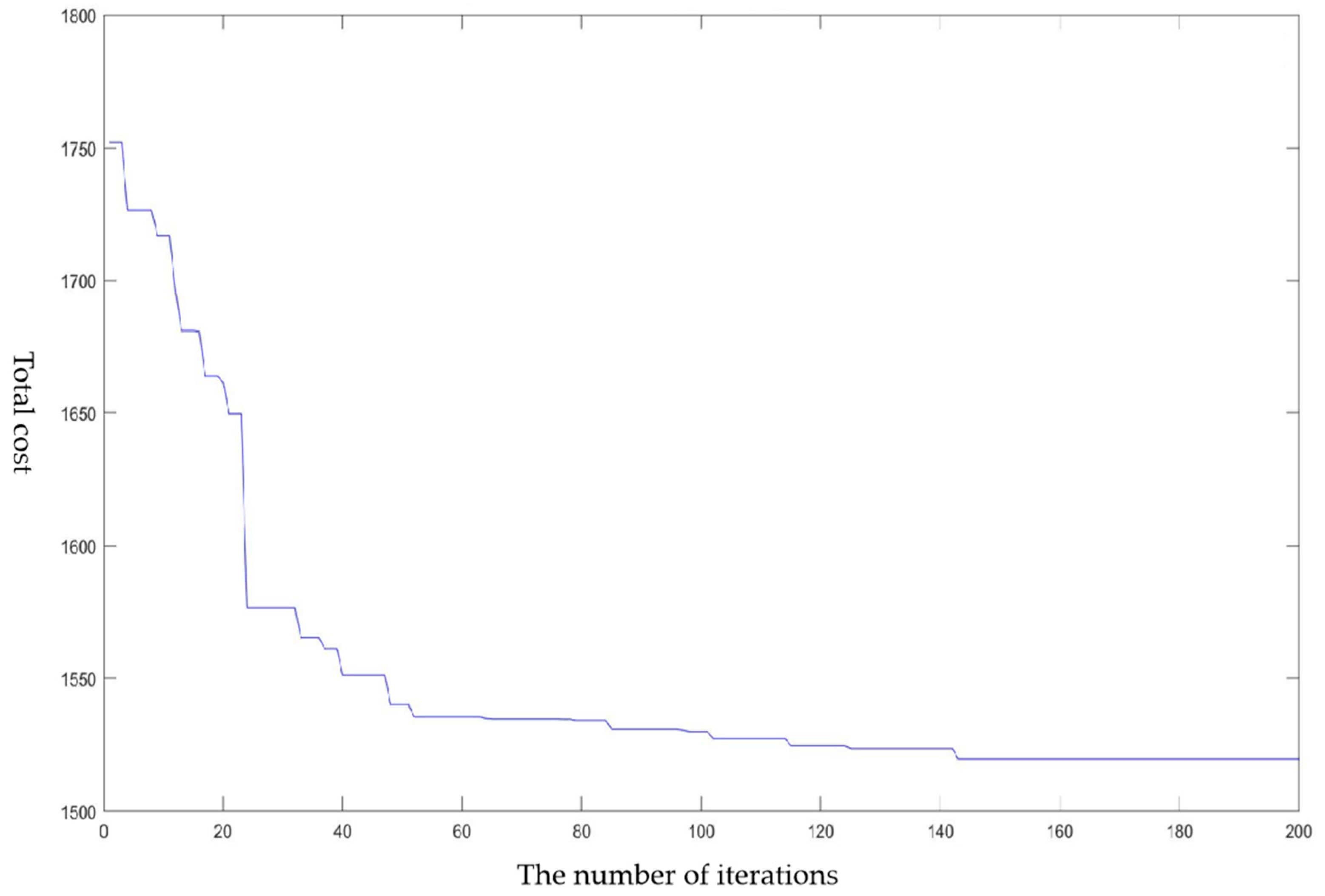
Figure 5 shows the convergence curve of the adaptability function while using the ant colony algorithm to solve the DRT based on the reservation scheduling model. The results show that the total cost of system operation gradually decreases with the increase in the number of iterations. The objective function reaches convergence in the 143rd generation, obtaining the optimal objective value, i.e., the minimum value of the total cost considering the vehicle size and mileage, CNY1519.52.

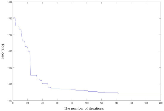
Figure 5. The convergence curve of the adaptability function for solving the model.

Table 5 shows the scheduling scheme results corresponding to the optimal target value. The vehicle scheduling scheme results show that only 16.67% of the vehicle scale can cover the demand for 180 trips in this time period, with 30 vehicles, 150 empty trips, and 131.95 km of total empty mileage.

Table 5. The scheduling scheme corresponding to the optimal target value.

Vehicle Number	Departure Task Chain	Deadhead Traveling Path (m)	Vehicle Size
1	11-48-58-173-41-45-147-63	853	Medium
2	46-52-20-149-72-148-19	0	Small
3	53-1-175-12-55-89-22-138-106	5042	Small
4	88-17-123-7-71-155-76-54	3343	Small
5	44-172-140-4-178-5-38	2996	Medium
6	96-80-23-37-109-164	3583	Small
7	8-158-176-87-107-65	2317	Small
8	157-77-122-39-166-9-170	1985	Medium
9	36-135-156-151-146-26-2-16	2101	Medium
10	162-127-131-116-137-154-121-145	6696	Medium
11	141-124-161-129-29-125-3-120	1761	Small
12	30-78-163-174-56-24-50-86-167	9401	Medium
13	117-74-47-34-171-43-59	13,273	Small
14	90-130-177-133-28-126-103	13,259	Small
15	168-64	1121	Small
16	73-114-70-6-108-180-100-51-160	2185	Large
17	33-10-42-95-139-105-35-136	9293	Medium
18	113-69-57-81-118-104-128	4878	Medium
19	61	0	Small
20	98	0	Small
21	27-84-179-31	1742	Medium
22	68-93-110-92-82-67-102	2306	Large
23	75-119	6062	Medium
24	159-142-85-13-144-15-152	2264	Large
25	60-111-14-21-97-143-91	10,714	Large
26	40-79-112-169-66-18-132	6595	Large
27	94-25-83-62-153	9919	Large
28	32-150-115-99	6044	Large
29	101-49	0	Large
30	134-165	2215	Large

If only the unilateral factor of vehicle number is considered without the deadhead traveling path factor, the results for the same case are compared in Table 6. The results show that compared with the scheduling solution that only considers the vehicle size unilaterally, the scheduling solution that integrates the vehicle size and mileage factors can reduce the total empty mileage of the vehicle chain by 23.34%, effectively reducing invalid empty trips and thus reducing the empty trip cost, while reducing the vehicle size to the same level. The above results prove the feasibility and effectiveness of this model algorithm for solving the DRT-based reservation scheduling problem.

Table 6. Comparison of results.

Considerations	Vehicle Number	Deadhead Traveling Path	Deadhead Traveling Costs
Vehicle number	30	162.97	282.95
Vehicle number + Empty mileage	30	131.95	228.52

5. Conclusions

DRT is of great significance for improving the competitiveness of public transportation and realizing green transportation. This paper proposes a DRT based on a reservation scheduling model by abstracting its problem’s essence through a directed acyclic graph. This model simultaneously takes into account realistic factors such as multiple vehicle sizes and the travel distance of vehicles and takes the minimization of the total operation cost as the optimization objective. An ant colony algorithm suitable for large-scale operations is designed to solve it. Finally, the effectiveness and advancement of the vehicle scheduling optimization model are verified based on the data of routes, stops, and demands using the Shanghai Huyi Highway Demonstration Line, a typical route of reservation-based customized buses, as a test case. The results show that the scheme can effectively control the vehicle size, reduce empty mileage, and improve the utilization rate of vehicle resources.

Owing to the complexity of the vehicle scheduling problem, there are also some weaknesses in this paper, such as idealizing the number of various vehicle sizes and the speed of vehicle operation, which greatly impact the scheduling scheme. Future research can start from the following aspects: firstly, the prediction of the running speed and arrival time of DRT needs to be more accurate. Secondly, more realistic factors, such as the limitation of the number of various vehicle sizes, the weather, and the impact of the stability of DRT on passengers. Finally, more efficient algorithms can be introduced to meet the speed and accuracy requirements of DRT.

References

- Flusberg, M. An innovative public transportatic on system for a smallcity: The Merrill, Wisconsin, case study. Transp. Res. Rec. 1976, 606, 54–59. [Google Scholar]
- Transportation Research Board; National Academies of Sciences, Engineering, and Medicine. Operational Experiences with Flexible Transit Services; The National Academies Press: Washington, DC, USA, 2004; pp. 18–19. [Google Scholar] [CrossRef]
- Zheng, H.; Zhang, X.C.; Wang, Z.M. Design of Demand-responsive Service by Mixed-type Vehicles. J. Transp. Syst. Eng. Inf. Technol. 2018, 8, 157–163. [Google Scholar] [CrossRef]
- Ghannadpour, S.F.; Noori, S.; Tavakkoli-Moghaddam, R.; Ghoseiri, K. A multi-objective dynamic vehicle routing problem with fuzzy time windows: Model, solution and application. Appl. Soft Comput. 2014, 14, 504–527. [Google Scholar] [CrossRef]
- Narayan, J.; Cats, O.; Oort, N.; Hoogendoorn, S. Integrated route choice and assignment model for fixed and flexible public transport systems. Transp. Res. Part C Emerg. Technol. 2020, 115, 102631. [Google Scholar] [CrossRef]
- Shen, C.; Cui, H.J. Optimization of Real-time Customized Shuttle Bus Lines Based on Reliability Shortest Path. J. Transp. Syst. Eng. Inf. Technol. 2019, 19, 99–104. [Google Scholar] [CrossRef]
- Ding, S. The Route Optimization Research of Flexible Feeder Transit System. Master’s Thesis, Shandong University, Jinan, China, 2016. [Google Scholar]
- Sun, B.; Wei, M.; Zhu, S.L. Optimal Design of Demand-Responsive Feeder Transit Services with Passengers’ Multiple Time Windows and Satisfaction. Future Internet 2018, 10, 30. [Google Scholar] [CrossRef]
- Lu, B.C.; Huang, J.Y.; Zhang, D.M. Research on Optimization of Station Demand-Responsivepublic Transit Dispatching System. J. Chongqing Inst. Technol. (Nat. Sci.) 2021, 35, 34–43. [Google Scholar] [CrossRef]
- Li, X.; Wang, T.Q.; Xu, W.H.; Li, H.; Yuan, Y. A novel model and algorithm for designing an eco-oriented demand responsive transit (DRT) system. Transp. Res. Part E Logist. Transp. Rev. 2022, 157, 102556. [Google Scholar] [CrossRef]
- Ma, C.X.; Wang, C.; Xu, X.C. A Multi-Objective Robust Optimization Model for Customized Bus Routes. IEEE Trans. Intell. Transp. Syst. 2021, 22, 2359–2370. [Google Scholar] [CrossRef]
- Qiu, F.; Li, W.Q.; Zhang, J. A dynamic station strategy to improve the performance of flex-route transit services. Transp. Res. Part C Emerg. Technol. 2014, 48, 229–240. [Google Scholar] [CrossRef]
- Bruni, M.E.; Guerriero, F.; Beraldi, P. Designing robust routes for demand-responsive transport systems. Transp. Res. Part E Logist. Transp. Rev. 2014, 70, 1–16. [Google Scholar] [CrossRef]
- Petit, A.; Ouyang, Y.F. Design of heterogeneous flexible-route public transportation networks under low demand. Transp. Res. Part C Emerg. Technol. 2022, 138, 103612. [Google Scholar] [CrossRef]
- Bakas, I.; Drakoulis, R.; Floudas, N.; Lytrivis, P.; Amditis, A. A Flexible Transportation Service for the Optimization of a Fixed-route Public Transport Network. Transp. Res. Procedia 2016, 14, 1689–1698. [Google Scholar] [CrossRef]
- Sun, J.Y.; Huang, J.L.; Chen, Y.Y.; Wei, P.Y.; Jia, J.L. Flexible Bus Route Optimization Scheduling Model for Multi-target Stations. J. Transp. Syst. Eng. Inf. Technol. 2019, 19, 105–111. [Google Scholar] [CrossRef]
- Wang, Z.W.; Yu, J.; Hao, W.; Chen, T.; Wang, Y. Designing High-Freedom Responsive Feeder Transit System with Multitype Vehicles. J. Adv. Transp. 2020, 2020, 8365194. [Google Scholar] [CrossRef]
- Wang, Z.W.; Chen, T.; Song, M.Q. Coordinated optimization of operation routes and schedules for responsive feeder transit under simultaneous pick-up and delivery mode. J. Traffic Transp. Eng. 2019, 19, 139–149. [Google Scholar] [CrossRef]
- Ren, J.X.; Chang, X.T.; Wu, W.T.; Jin, W.Z. Demand Responsive Feeder Transit Scheduling Considering Candidate Stops and Full-service Process. J. Transp. Syst. Eng. Inf. Technol. 2023, 23, 202–214. [Google Scholar] [CrossRef]
- Wang, L.; Zeng, L.; Ma, W.J.; Guo, Y.H. Integrating passenger incentives to optimize routing for demandresponsive customized bus systems. IEEE Access 2021, 9, 21507–21521. [Google Scholar] [CrossRef]
- Shen, S.Y.; Ouyang, Y.F.; Ren, S.; Zhao, L.Y. Path-Based Dynamic Vehicle Dispatch Strategy for Demand Responsive Transit Systems. Transp. Res. Rec. 2021, 2675, 948–959. [Google Scholar] [CrossRef]
- Ayadi, M.; Chabchoub, H.; Yassine, A. An exact method for the multi-vehicle static demand responsive transport problem based on service quality: The case of one-to-one. In Proceedings of the 2014 International Conference on Advanced Logistics and Transport (ICALT), Hammamet, Tunisia, 1–3 May 2014; pp. 308–313. [Google Scholar] [CrossRef]
- Qiu, X.Q.; Feuerriegel, S.; Neumann, D. Making the most of fleets: A profit-maximizing multi-vehicle pickup and delivery selection problem. Eur. J. Oper. Res. 2016, 259, 155–168. [Google Scholar] [CrossRef]
- Mohammad, R.; Ahmed, G. A branch-and-price algorithm for a vehicle routing with demand allocation problem. Eur. J. Oper. Res. 2019, 272, 523–538. [Google Scholar] [CrossRef]
- Lysgaard, J. Reachability cuts for the vehicle routing problem with time windows. Eur. J. Oper. Res. 2006, 175, 210–223. [Google Scholar] [CrossRef]
- Mak, V.; Ernst, A.T. New cutting-planes for the time- and/or precedence-constrained ATSP and directed VRP. Math. Methods Oper. Res. 2007, 66, 69–98. [Google Scholar] [CrossRef]
- Lyu, Y.; Chow, C.Y.; Lee, V.C.S.; Joseph, K.Y.N.; Li, Y.H.; Zeng, J. CB-Planner: A bus line planning framework for customized bus systems. Transp. Res. Part C Emerg. Technol. 2019, 101, 233–253. [Google Scholar] [CrossRef]
- Cimen, M.; Soysal, M. Time-dependent green vehicle routing problem with stochastic vehicle speeds: An approximate dynamic programming algorithm. Transp. Res. Part D Transp. Environ. 2017, 54, 82–98. [Google Scholar] [CrossRef]
- Nie, J.R. Research on Flexible Feeder Transit Route Planning Based on Improved Tabu Search Algorithm. Master’s Thesis, Tsinghua University, Beijing, China, 2017. [Google Scholar]
- Jin, W.Z.; Ren, J.X.; Wu, W.T. Demand Responsive Feeder Transit Scheduling with Flexible Service Quality. In Proceedings of the 2020 IEEE 5th International Conference on Intelligent Transportation Engineering (ICITE), Beijing, China, 11–13 September 2020; pp. 565–569. [Google Scholar] [CrossRef]
- Sun, B.; Wei, M.; Yang, C.F.; Cender, A. Solving demandresponsive feeder transit service design with fuzzy travel demand: A collaborative ant colony algorithm approach. J. Intell. Fuzzy Syst. 2019, 37, 3555–3563. [Google Scholar] [CrossRef]
- Jin, W.Z.; Hu, W.Y.; Deng, J.Y.; Luo, C.Y.; Wei, L.H. Flexible scheduling model of demand response transit based on hybrid algorithm. J. South China Univ. Technol. (Nat. Sci. Ed.) 2021, 49, 123–133. [Google Scholar] [CrossRef]
- He, M.; Li, M.X.; Shui, W.B.; Qian, H.M. Influence of Reliability and Comfort on Responsive Custom Bus Route Design. J. Highw. Transp. Res. Dev. 2019, 36, 145–151. [Google Scholar] [CrossRef]
- Perera, T.; Prakash, A.; Srikanthan, T. Genetic Algorithm based Dynamic Scheduling of EV in a Demand Responsive Bus Service for First Mile Transit. In Proceedings of the 2019 IEEE Intelligent Transportation Systems Conference (ITSC), Auckland, New Zealand, 27–30 October 2019; pp. 3322–3327. [Google Scholar] [CrossRef]
Disclaimer/Publisher’s Note: The statements, opinions and data contained in all publications are solely those of the individual author(s) and contributor(s) and not of MDPI and/or the editor(s). MDPI and/or the editor(s) disclaim responsibility for any injury to people or property resulting from any ideas, methods, instructions or products referred to in the content. |
© 2024 by the authors. Licensee MDPI, Basel, Switzerland. This article is an open access article distributed under the terms and conditions of the Creative Commons Attribution (CC BY) license (https://creativecommons.org/licenses/by/4.0/).