Featured Application
This study presents a new pullback load calculation model from the perspective of pipe–borehole wall contact.
Abstract
Pipeline pullback load is a crucial basis for drill rig selection and pipeline strength design. This paper presents a new pullback load calculation model from the perspective of pipe–borehole wall contact. The pipe–borehole wall contact analysis includes the distribution of contact pressure and the relationship between the external load and compressive displacement. The friction force between the pipe and the borehole wall was calculated based on the pipe–borehole wall contact analysis and adhesion theory without depending on the empirical friction coefficient. The effects of the eccentricity were also considered when calculating the fluid drag force. Through case studies, we verified the applicability of the model and discussed the possible reasons for the errors between the theoretical and field-measured results. This study can provide a helpful tool for analyzing the pipe–borehole wall contact and pullback loads for horizontal directional drilling.
1. Introduction
Horizontal directional drilling (HDD) is a trenchless pipeline installation technology that has rapidly developed in recent years. HDD is widely used to install oil and gas pipelines, power cables, and municipal pipe networks [1,2]. Its advantages of high efficiency, environmental protection, and reduced ground excavation have made this technology increasingly crucial for large-scale infrastructure projects [3].
HDD technology is a large-scale project that combines multiple technologies, equipment, and disciplines [4]. The pipeline installation process consisted of pilot boring, pre-reaming, and pullback [5]. The prediction accuracy of pullback loads affects the drill rig selection and pipeline strength design, which is essential for ensuring the safe installation of pipelines [6]. In particular, for an increasing number of large-scale pipeline installation projects, because of the long length and large diameter of the installed pipelines, if the pullback load calculation is not accurate, sticking of the pipeline can easily occur, resulting in substantial economic losses [3].
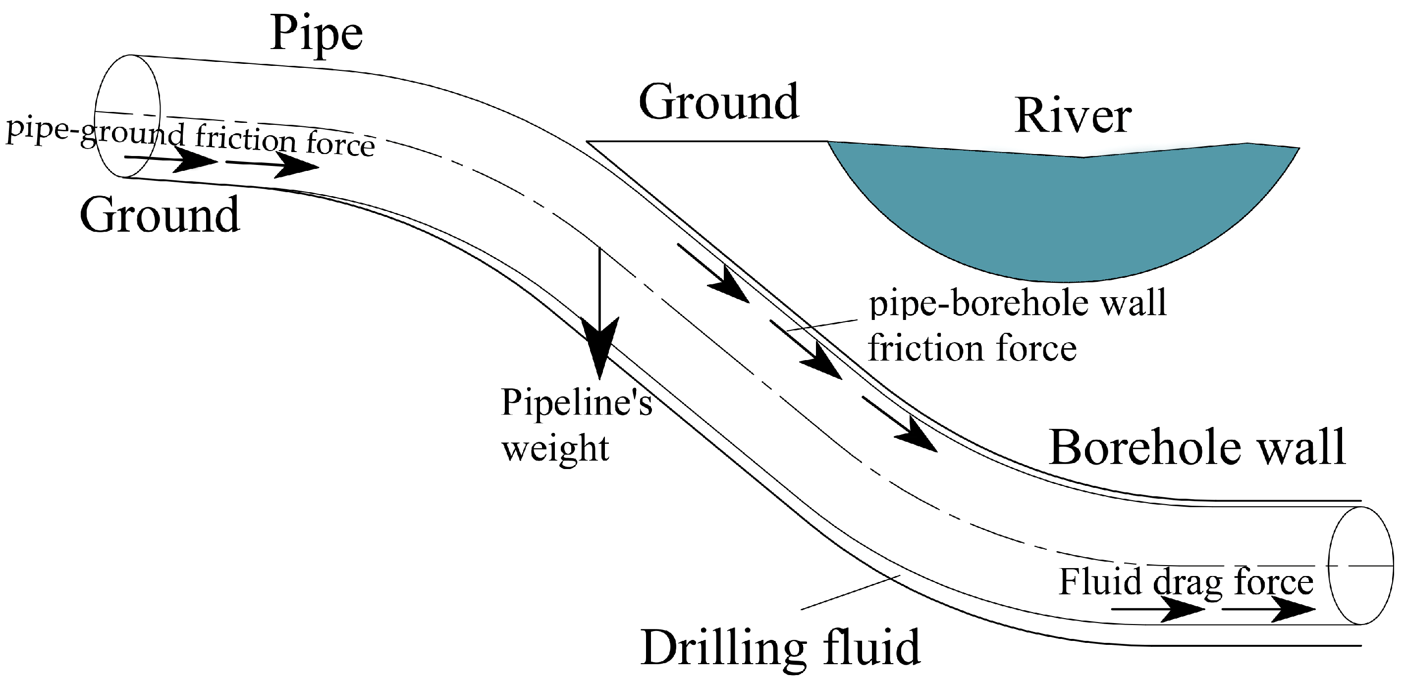
The forces acting on a pipeline during pullback are complex. Calculating pullback loads involves knowledge of tribology and fluid, elastic, and soil mechanics. The composition of the pipeline pullback loads can be summarized into the following four parts [7,8]: (1) the friction force between the pipeline and ground surface or roller, (2) the friction force between the pipeline and borehole wall (including the friction force caused by the net weight of the pipeline and capstan effect), (3) the drag force between the pipeline and drilling fluid, and (4) the pipeline’s weight. Figure 1 shows the forces acting on a pipeline during the pullback process. The resultant of these forces in the pullback direction constitutes the pullback load.

Figure 1.
Forces acting on a pipeline during the pullback process.
To calculate pullback loads in HDD, scholars have conducted extensive research and proposed practical methods that promote the advancement of HDD technology [8,9,10,11,12,13,14]. The Phillips Driscopipe model [9] considers the pipe–borehole wall friction caused by the net weight of the pipeline. This friction force is considered to be the pullback load required for pipeline installation. To maintain the stability of the borehole wall, the HDD borehole was filled with a drilling fluid. Previous studies have found that drilling fluid drag force is an essential component of pullback loads. The CNPC method [12] further considers the drilling fluid drag force, which is calculated by multiplying the outer surface area of the pipeline in the borehole by the viscosity coefficient ks. The calculation of pipe–borehole wall friction force in the CNPC method aligns with that of the Phillips Driscopipe model. The HDD borepath generally comprises straight and curved segments. When the pipeline crosses the curved segment, owing to the change in the direction of the pilot borehole, the external load applied to the borehole wall increases, known as the capstan effect. The increased external load resulted in additional pullback loads. The PRCI model [14] and ASTM model [11] consider the impact of the capstan effect. In addition, the drilling fluid drag force in the ASTM model is calculated by considering a balance of the forces acting on the fluid annulus in the borehole due to the pressure difference and the lateral shear forces acting on the pipe and borehole walls. The pressure difference is estimated to be 70 kPa. Polak et al. [13], Cheng et al. [8], and Cai et al. [15] further improved the calculation of drilling fluid drag force. The pressure difference is no longer estimated as a specific value. The drilling fluid was assumed as a non-Newtonian fluid. Formulas for the pressure difference and pipe wall shear stress in a concentric annulus were derived based on fluid mechanics [8,13,15]. The rheological characteristics have a considerable influence on drilling fluid drag force. Deng et al. [16] investigated the rheological characteristics of drilling fluids with varying bentonite concentrations. Their findings indicate that both the Bingham and Herschel–Bulkley models can describe the behavior of drilling fluids used in HDD. Faghih et al. [17] conducted a parameter sensitivity analysis on the effect of rheological parameters on the drilling fluid drag force. The results showed that the ratio of borehole to pipe radius and rheological characteristics significantly affect the drilling fluid drag force.
At present, there is a lack of research on the pipe–borehole wall contact in HDD. The calculation of pipe–borehole wall friction force in engineering practice relies on the empirical friction coefficient which is determined experimentally rather than predicted using physical models [18]. As a significant improvement over the classical friction laws, it is now widely accepted that the friction force is proportional to the real contact area. This has been confirmed by many experiments [19,20,21], and much work has been conducted based on this hypothesis [19,20,21,22,23,24]. Therefore, the understanding of friction based on the mechanics of contact [25] can provide a new idea for studying the friction force between the pipeline and borehole wall during pipeline pullback operation.
Additionally, the pressure difference has a significant impact on the fluid drag force when using ASTM model. The pressure difference of the annulus is related to the annulus size, flow rate, and drilling fluid parameters [11]. Taking the pressure difference as a particular value may cause errors in calculating fluid drag force because the related parameters differ for various HDD projects. Moreover, pipelines in the borehole are more likely to contact the borehole wall than to be located at the center of the borehole [6]. The eccentric characteristics of the annulus are essential for improving the accuracy of fluid drag force.
This study proposes a new theoretical model for calculating pullback loads in HDD. Based on a large number of finite element method (FEM) analysis results, formulas for the contact pressure distribution between the pipe and borehole wall and the external load–displacement relationship were derived to analyze the pipe–borehole wall contact. The pipe–borehole wall friction force was calculated based on the pipe–borehole wall contact analysis and adhesion theory without depending on the empirical friction coefficient. The fluid drag force was calculated based on the ASTM model, and the effects of the annulus size, flow rate, drilling fluid parameters, and eccentricity were considered. The proposed model, ASTM model, and PRCI model were used to analyze two HDD installations. The model predictions were compared with the field-measured results and the applicability of the proposed method was discussed.
2. Analysis of Pipe–Borehole Wall Contact
During the pullback process, the pipeline contacts the borehole wall under the action of external load (including the contributions from buoyancy, gravity, and capstan effect). When the direction of the external load is upward, the pipeline may contact the upper wall of the borehole. Conversely, the pipeline may have been in contact with the bottom of the borehole. The pipe–borehole wall contact analysis under the external load is an axisymmetric mechanical problem because the pipeline and borehole have approximately circular cross-sections. Figure 2 shows the contact state between the pipeline and borehole wall by taking an upward external load (often occurring without buoyancy control) as an example. P signifies the external load per unit length of the pipeline. R1 and R2 denote the radii of the pipe and borehole, respectively. β represents the angle at which points on the interface depart from the central line. ε stands for the semi-angle of contact corresponding to the whole contact arc. l signifies the semi-chord length corresponding to the angle ε. ΔR represents the radial clearance of the pipe and borehole, ΔR = R2 − R1. δ denotes the compressive displacement.
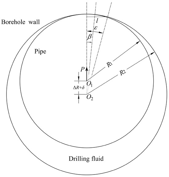
Figure 2.
Schematic of the pipe–borehole wall contact.
2.1. Classical Contact Models
The contact between the pipe and borehole wall shown in Figure 2 is a typical internal cylinder contact problem. Researchers have developed different methods for determining the contact pressure distribution and external load–displacement relationship for the internal cylinder contact problem. It should be noted that, unlike classical contact models, the HDD pipe–borehole wall contact model needs to consider the effect of drilling fluid pressure. At this point, the maximum contact pressure between the pipe and the borehole wall changes. Therefore, in this paper, the maximum contact pressure without drilling fluid pressure is denoted as q0, while the maximum contact pressure in HDD (considering the drilling fluid pressure) is denoted as p0. The relationship between q0 and p0 will be discussed in the following sections.
2.1.1. Hertz Model
Hertz theory is one of the most common methods for internal cylinder contact problems. In the Hertz model, the contact pressure distribution is assumed as follows [26]:
where pc signifies the contact pressure, q0 denotes the maximum contact pressure without drilling fluid pressure, x represents the distance between the point on the interface and symmetry axis; n signifies the pressure distribution exponent, n = 1/2 in the Hertz model.
The maximum contact pressure between the two cylinders is expressed as follows [26]:
where E* represents the equivalent elastic modulus, which is defined as follows:
where E1 and E2 denote the elastic modulus of the inner and outer cylinders, respectively; v1 and v2 stand for the Poisson’s ratio of the inner and outer cylinders, respectively.
It is noteworthy that Equation (2) cannot be directly used to calculate the maximum contact pressure because the compressive displacement δ and the semi-chord length of contact l are unknown.
The compressive displacement δ can be calculated as follows [27]:
The semi-chord length of contact l in the Hertz model can be determined by the geometric relationship between the semi-chord length of contact l and compressive displacement δ as follows [27]:
where R denotes the relative curvature of the contact and is defined as follows:
Substituting Equations (4) and (5) into Equation (2), the maximum contact pressure in the Hertz model can be obtained as follows:
2.1.2. Persson Model
Assuming that the radial displacement of the contact area was independent of the tangential displacement, Persson derived the geometric relationship of the contact area as follows [28]:
where u1 and u2 denote the radial displacements of the inner and outer cylinders at the contact point, respectively.
Ciavarella et al. [29,30] developed the Persson theory and proposed a completely closed-form solution to the contact problem of cylinders with clearance. The maximum contact pressure was calculated using the following equation:
where B = (2b4 + 2b2 − 1)/(b4 + b2), b = tan(ε/2). The auxiliary variable b can be obtained by solving the following nonlinear equation:
where is the modified Young’s modulus; α0, β0 is Dundurs’s material parameters. The definitions of the parameters in Equation (10) can be found in the research of Ciavarella et al. [29]. The contact pressure distribution of the Persson model aligns with that of the Hertz model (Equation (1)).
2.1.3. Liu Model
The Winkler elastic foundation model is commonly used to describe the outer cylinder in cylinder contact problems [31,32,33]. Based on the Winkler elastic foundation model and the FEM, Liu et al. [31] developed a method for calculating the maximum contact pressure as follows:
where the compressive displacement δ can be calculated by the following formula:
The contact pressure distribution of the Liu model also aligns with that of the Hertz model (Equation (1)).
Notably, these models are based on different theoretical assumptions and have different application scopes. The Hertz model assumes that the pressure distribution exponent n is 1/2. The shape and size of the bodies and how they are supported must be accounted for [33]. Liu et al. [31] further examined the applicability of the Hertz model and found that the Hertz model is only applicable when there is a large clearance between cylinders and the external load is small. Persson’s model is based on a geometric relationship (Equation (8)) of the contact area. When ΔR is large, this relationship also has significant errors at the edge of the contact area (β = ε). Liu’s model assumes that the displacement of the elastic foundation at the vertex of the wedge is half the compressive displacement; however, this ratio may change when the cylinder size or external load changes [34].
Unlike common internal cylinder contact problems (such as friction pairs) in mechanical systems, the pipe–borehole wall contact in HDD has a large clearance (the order of magnitude is typically 10–102 mm), and the borehole wall is subjected to drilling fluid pressure. Therefore, it is necessary to find a method for determining the contact pressure distribution and external load–displacement relationship suitable for HDD. This topic will be discussed in the following section.
2.2. HDD Pipe–Borehole Wall Contact Model
The contact pressure distribution can be expressed as follows [33]:
There are two parameters that need to be determined in Equation (13): the maximum contact pressure p0 and the pressure distribution exponent n. The following sections will explain how to determine these two parameters.
2.2.1. Maximum Contact Pressure in HDD
Compared to analytical methods, FEM is not limited by the assumptions of contact pressure distribution and geometric relationships and is widely used in contact analysis [31,34,35,36,37,38,39]. This study used FEM to investigate the pressure distribution and external load–compressive displacement relationship for the pipe–borehole wall contact in HDD projects. The details of the FEM model are provided in Appendix A. The calculation parameters are listed in Table 1, and the range of parameters is based on the HDD operating conditions.

Table 1.
Parameters values used for FEM simulations.
Hu et al. [34] showed no significant difference between the elastic and elastic–plastic analysis results when the external load P was small. Taking the 900 mm diameter HDPE pipe as an example, the order of magnitude of the external load, P, was approximately 1 N/mm. In addition, we conducted an elastic–plastic analysis for No. 1–3 test conditions (Table 1). These results were consistent with those of the elastic analysis, and no plastic deformation occurred. Therefore, this contact analysis assumes that the pipe and borehole walls are isotropic elastic bodies.
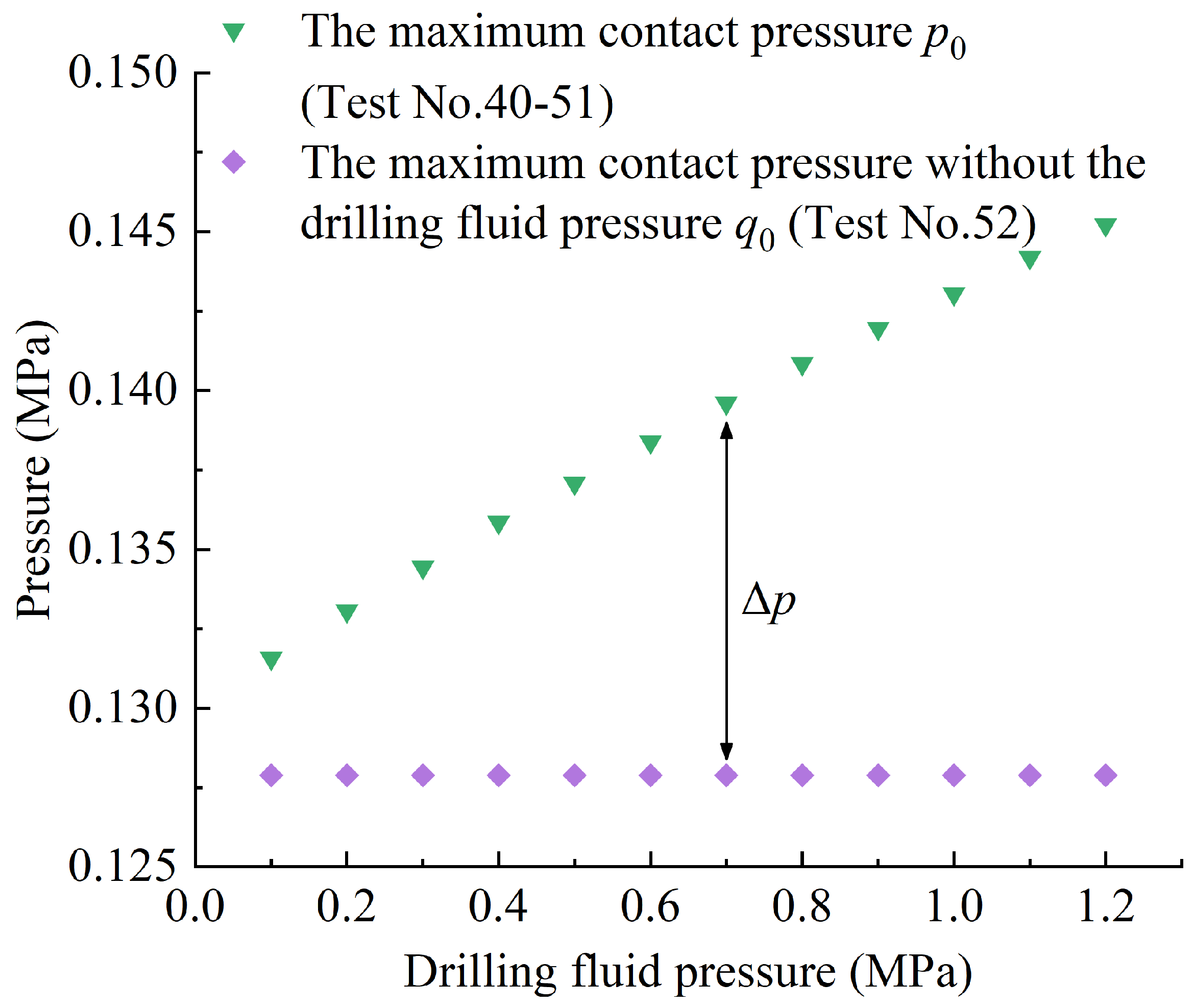
Figure 3 shows the change in the maximum contact pressure when only the drilling fluid pressure σ0 is changed (No. 40–52 tests in Table 1). It can be observed that the drilling fluid pressure affects the maximum contact pressure; the greater the drilling fluid pressure, the more significant the impact. Therefore, it is necessary to consider the influence of the drilling fluid pressure in HDD pipe–borehole wall contact analysis. Figure 3 also shows that the drilling fluid pressure σ0 results in a maximum contact pressure increment Δp of q0 (the maximum contact pressure without the drilling fluid pressure). The maximum contact pressure p0 in HDD pipe–borehole wall contact can be represented as follows:
where Δp stands for the maximum contact pressure increment caused by the effect of drilling fluid pressure.
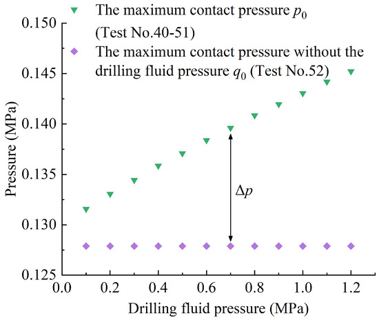
Figure 3.
Effect of drilling fluid pressure on maximum contact pressure.
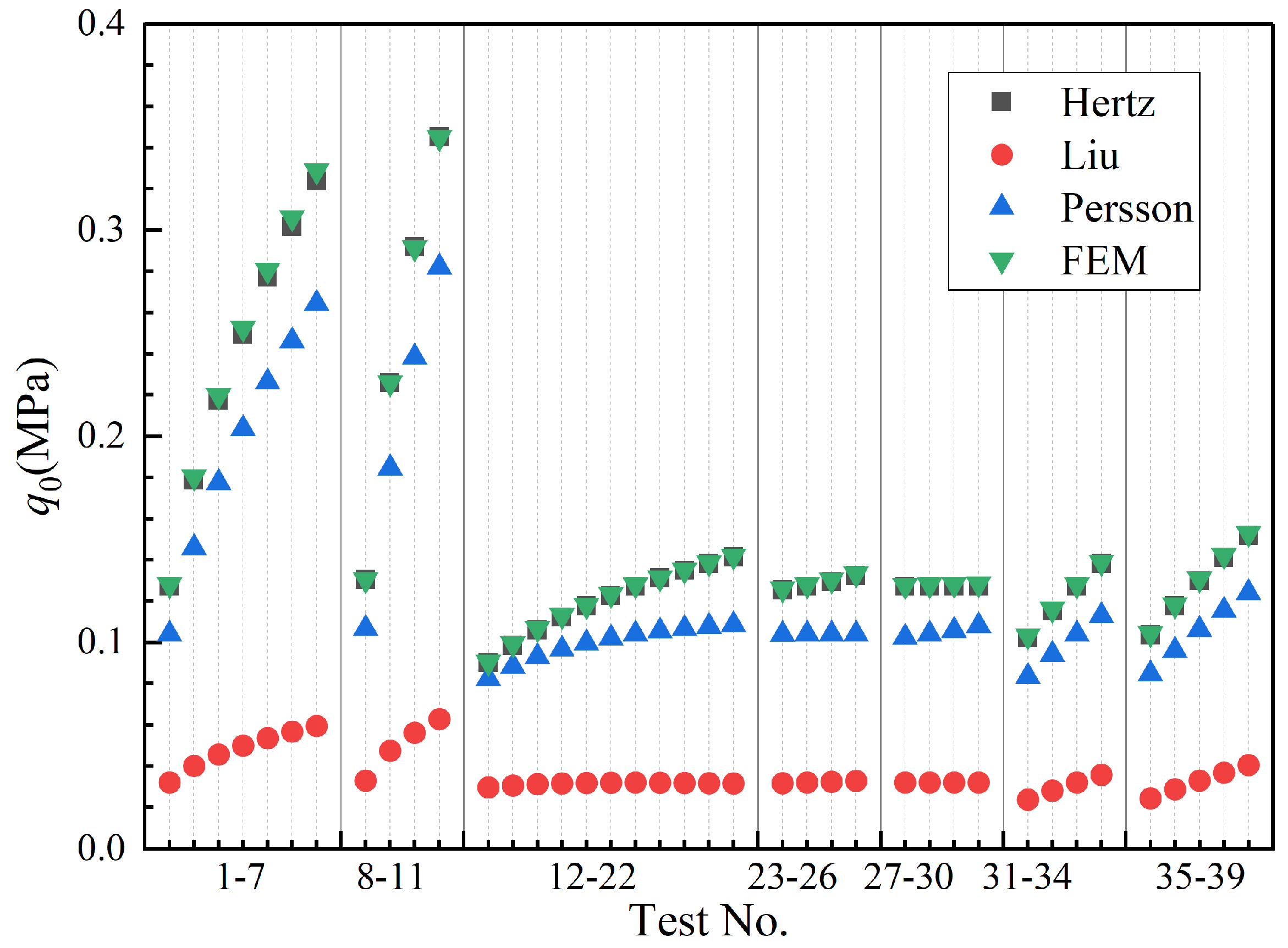
Figure 4 shows the maximum contact pressure without drilling fluid pressure (q0) calculated by different methods. The equations of the classical contact models have been introduced in the previous section. As depicted in Figure 4, the Hertz model had the smallest error in calculating q0, and the q0 variation law of the Hertz model was also consistent with the FEM results. Therefore, the Hertz model was used to calculate the maximum contact pressure without drilling fluid pressure q0:
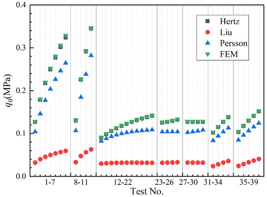
Figure 4.
Comparison of maximum contact pressure without drilling fluid pressure calculated by different models.
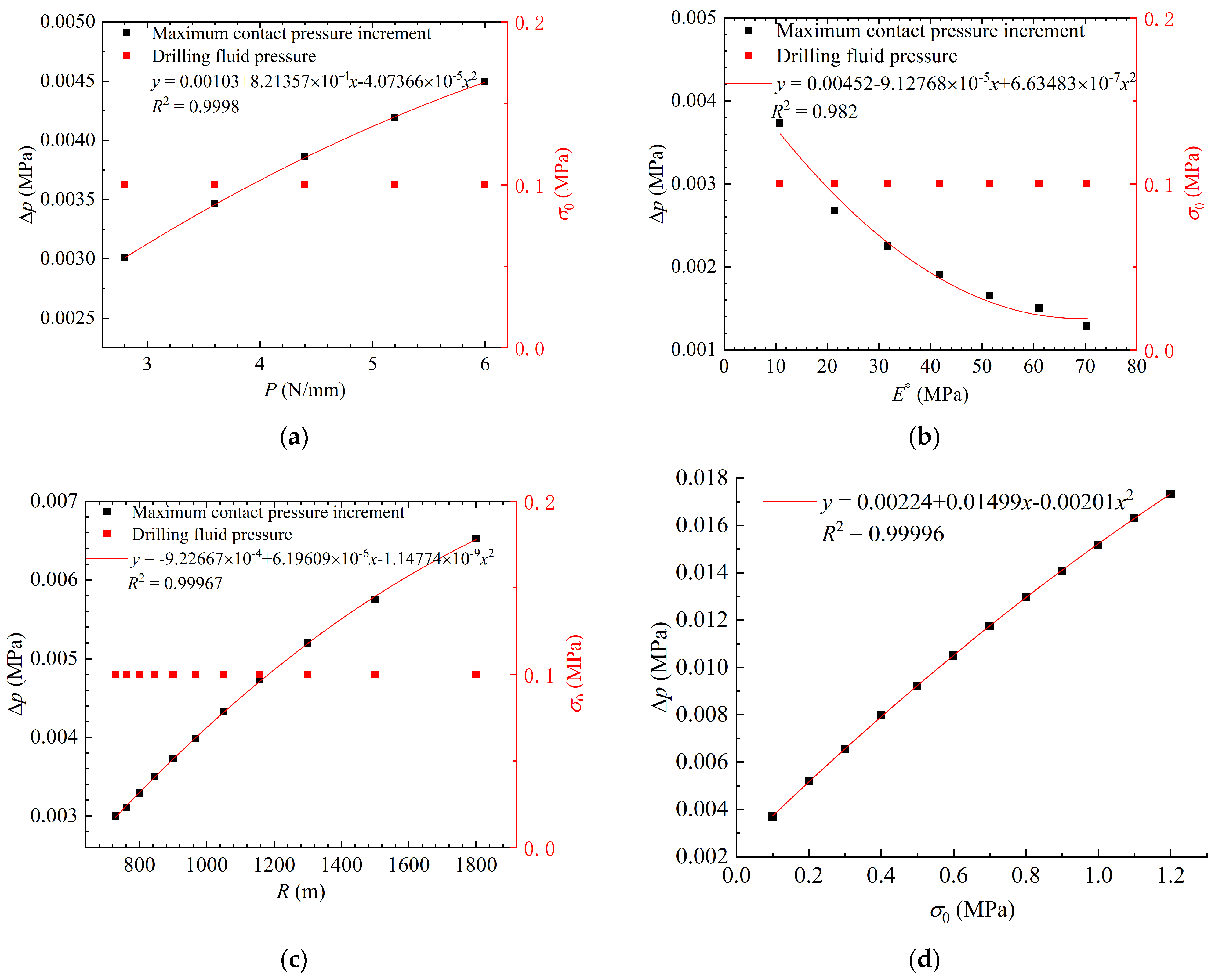
According to Equations (14) and (15), the maximum contact pressure p0 is related to the external load P, equivalent elastic modulus E*, equivalent radius R, and drilling fluid pressure σ0. To study the relationship between the maximum contact pressure increment Δp and the above parameters, the maximum contact pressure increment Δp under different parameters was calculated using FEM. The results are shown in Figure 5.
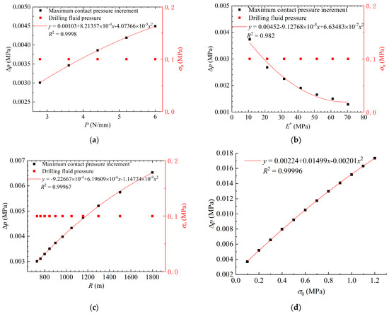
Figure 5.
Relationship between contact pressure increment and related parameters: (a) external load; (b) equivalent elastic modulus; (c) relative curvature of the contact; (d) drilling fluid pressure.
As illustrated in Figure 5, a second-order polynomial effectively describes the relationship between the maximum contact pressure increment Δp and each of the related parameters (P, E*, R, σ0). Additionally, compared to linear polynomials, the second-order polynomial fitting results exhibit smaller residuals and a higher R-squared value. Although higher-order polynomials may provide a better fit, they often lead to overfitting. Therefore, the second-order polynomial offers an optimal balance between fitting accuracy and model simplicity. In this study, the second-order polynomial was used to describe the relationship between the maximum contact pressure increment Δp and each of the related parameters. The equation is as follows:
where Ai (i = 1, 2 … 8) is the coefficient required to be determined/fitted, A0 represents the theoretical baseline of the system, which is used to adjust and calibrate the overall level of the model; A1, A3, A5, and A7 indicate the linear influence of E, R, σ0, and P on the maximum contact pressure increment, respectively; A2, A4, A6, and A8 reflect the nonlinear quadratic effect of E, R, σ0, and P on the maximum contact pressure increment, respectively.
Using data shown in Figure 5 and applying the nonlinear regression analysis method, it was found that, for most materials, geometric dimensions, and loads in HDD projects, the values of Ai (i = 1, 2, … 8) listed in Table 2 fit the results well. The mean squared error of this fitting is 2 × 10⁻⁴. The confidence interval is also shown in Table 2.
Table 2.
Ai values and 95% confidence interval.
The maximum contact pressure p0 can be obtained by substituting Equations (15) and (16) into Equation (14):
where P can be calculated by subtracting the gravity from the buoyancy acting on the pipe per unit volume, E* can be obtained by Equation (3), R can be calculated by Equation (6), and the values of Ai (i = 1, 2 …8) are listed in Table 2.
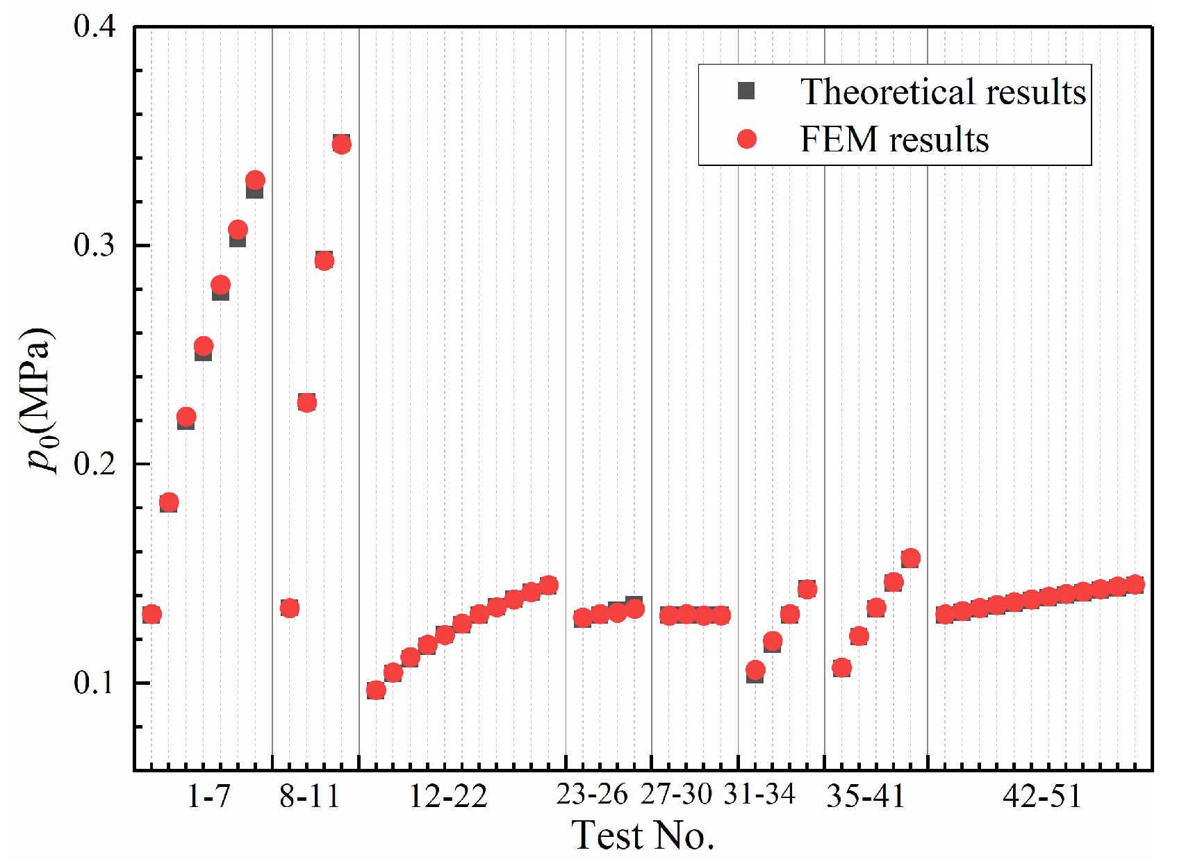
Figure 6 shows a comparison of the maximum contact pressure p0 between the theoretical result calculated by Equation (17) and the FEM results. It can be seen that the theoretical results are very close to the FEM results when considering the effect of drilling fluid pressure. The average absolute and relative errors for the 51 tests were 0.001 MPa and 0.6%, respectively.
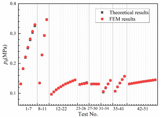
Figure 6.
Comparison between theoretical and FEM results of the maximum contact pressure p0.
2.2.2. Pressure Distribution Exponent in HDD
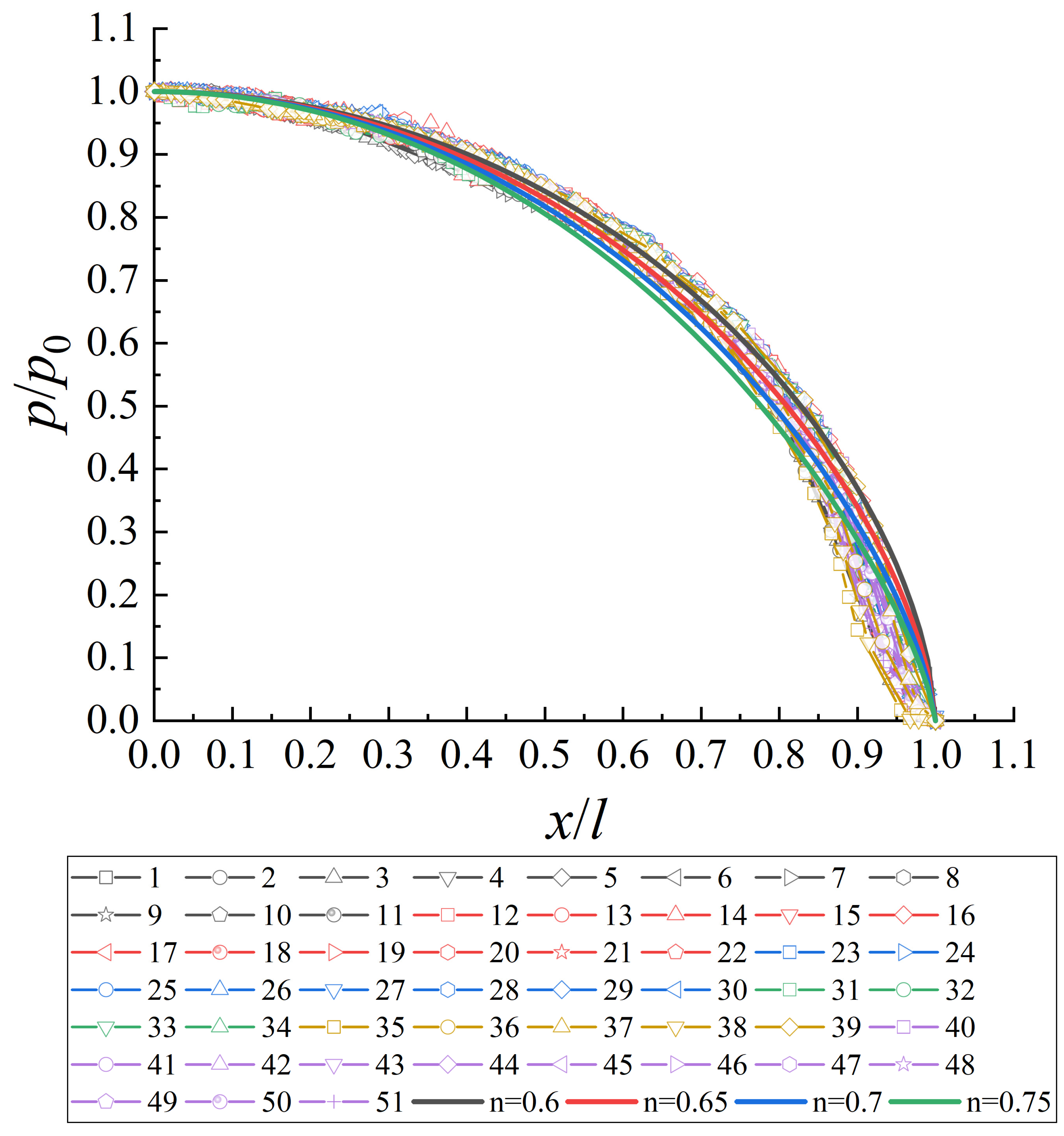
The pressure distribution exponent n determines the distribution form of contact pressure. For internal cylinder contact, Hertz distribution, which has an elliptic form (n = 1/2), is widely used. The pressure distribution exponent n can also be obtained through numerical fitting [39]. Considering the limitations of the Hertz model and the complexity of the contact in HDD, using numerical fitting to obtain n is more suitable for HDD pipe–borehole wall contact analysis. The distribution of the contact pressure for 51 different tests is shown in Figure 7. It is evident that the exponential function (Equation (13)) can better describe the distribution of the contact pressure. The value range of the exponent n in HDD is generally between 0.6 and 0.75.
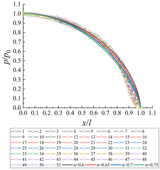
Figure 7.
Distribution of the contact pressure.
2.2.3. External Load–Displacement Relationship
A relationship between the external load P, maximum contact pressure p0, and the semi-chord length of contact l can be obtained by integrating the contact pressure distribution formula (Equation (13)):
Substituting Equation (14) into Equation (18) yields
where
Here, Γ denotes the gamma function, particularly if n = 1/2, B = π/4.
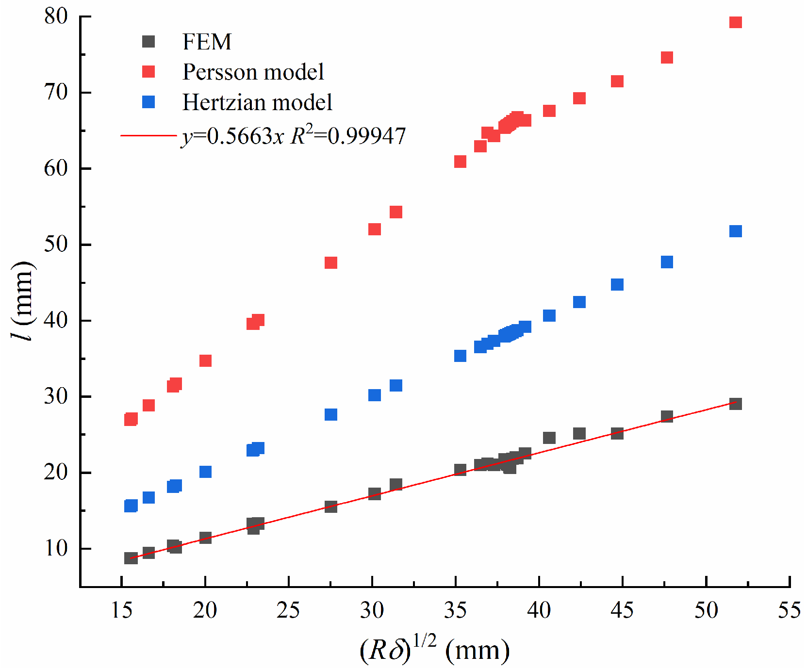
The analysis of the FEM results reveals that for the HDD pipe–borehole wall contact problem, there are significant errors (see Figure 8) when using the Hertz model (Equation (5)) or Persson model (Equation (8)) to describe the geometric relationship between the semi-chord length l and the compressive displacement δ. Notably, both the FEM and Hertz model results showed a linear relationship. Therefore, the Hertz model was modified to express the geometric relationship of the HDD pipe–borehole wall contact as follows:
where k is a dimensionless coefficient fitted in Figure 8 with a value of 0.5663.
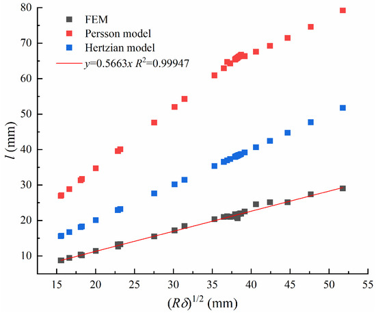
Figure 8.
Relationship between semi-chord length and compressive displacement.
Figure 8 shows the geometric relationship between the semi-chord length l and the compressive displacement δ. It can be seen that Equation (21) fits the FEM results well. Substituting Equation (21) into Equation (19), the relationship between the external load P and the compressive displacement δ is obtained as follows:
This section establishes the HDD pipe–borehole wall contact model, which forms the basis for calculating pipe–soil friction from a contact perspective.
3. Analytical Model for Calculating Pipe Pullback Loads
3.1. Pipe–Borehole Wall Friction Force
According to the adhesion theory developed by Bowden and Tabor, friction is primarily caused by adhesive interactions in the actual contact area [40]. The pipe–borehole wall friction force per unit length of pipe Ts can be expressed as follows [19]:
where τs is the shear (or friction) stress to break the junction (or adhesion), and Ar is the real contact area.
The shear stress τs can be expressed as [41]
where τf is the shear strength of the borehole wall.
The real contact area ratio α can be defined as [25]
where Ap is the projected area of the pipe–borehole wall contact area.
Correspondingly, the real contact area per unit length of the pipe is
According to the Mohr–Coulomb criterion, the shear strength of the borehole wall is defined as
where c denotes the cohesion; φ represents the internal friction angle; σa signifies the normal stress, and σa = P/Ar. It should be noted that the drilling fluid will generate a bentonite mud film on the borehole wall. As the part comes into contact with the pipeline, the cohesion and internal friction angle of the bentonite mud film are used when calculating the pipe–borehole wall friction force.
By substituting Equations (22), (24)–(27) into Equation (23), the formula for the pipe–borehole wall friction force per unit pipe length Ts can be obtained as follows:
It can be seen that the pipe–borehole wall friction force calculated through Equation (28) does not require an empirical friction coefficient.
3.2. Drilling Fluid Drag Force
The ASTM model calculates the drilling fluid drag force Tif by considering a balance of the forces acting on the fluid annulus in the borehole due to the pressure difference and the lateral shear forces acting on the pipe and borehole walls [11]:
The pressure difference ΔPf is estimated to be a constant value (70 kPa), which may cause errors in calculating fluid drag force because the related parameters differ for various HDD projects.
This model calculates the drilling fluid drag force based on the ASTM model, but the pressure difference is not estimated to be a constant value. The pressure difference of the annulus is related to the annulus size, flow rate, and drilling fluid parameters. Previous studies have demonstrated that drilling fluid typically behaves as a non-Newtonian fluid with a yield point. The Bingham model effectively describes the rheological characteristics of drilling fluids [16]. Therefore, the Bingham model was used to describe the drilling fluid in this study. The pressure difference ΔPf required for the laminar flow of Bingham fluid in an eccentric annulus can be expressed as follows [42,43]:
where ΔPfc represents the pressure difference in the concentric annulus; μ denotes the dynamic viscosity of drilling fluid; v stands for the flow velocity of drilling fluid; τ0 signifies the yield point of drilling fluid; S represents the length of the pipeline entering the borehole; and C denotes the correction factor, which is related to the eccentricity e and the overcut ratio R2/R1.
The correction factor C can be calculated by the following formula [43]:
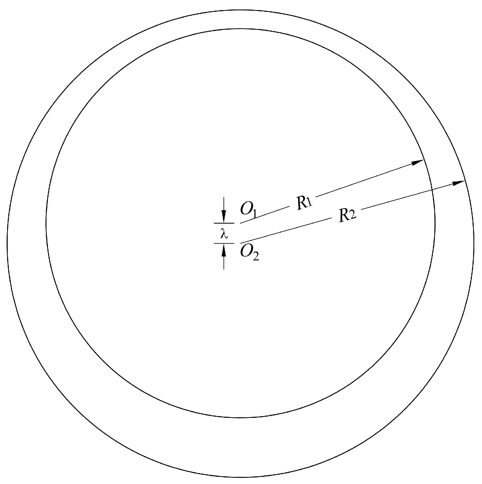
A schematic of the eccentric annulus is presented in Figure 9. Eccentricity e is defined as follows:
where λ is the distance between the centers of the pipe and the borehole.

Figure 9.
Schematic of the eccentric annulus.
The drilling fluid drag force Tif can be obtained by substituting Equation (30) into Equation (29):
The calculation of the drilling fluid drag force in this model considers the effects of the annulus size, flow rate, drilling fluid parameters, and eccentricity.
3.3. Pipeline Pullback Loads
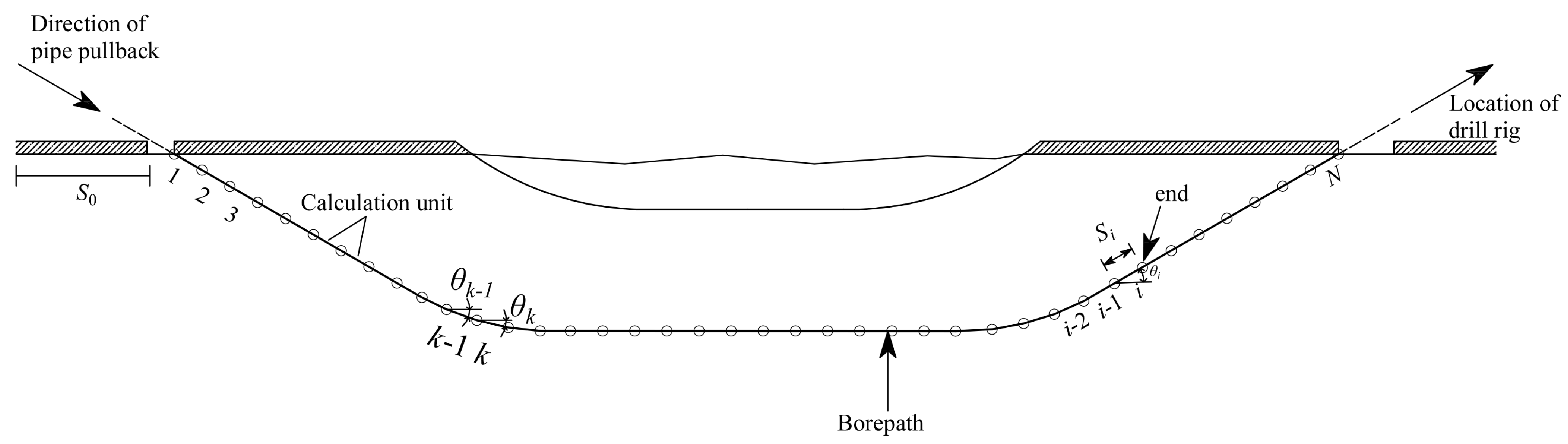
During pipeline pullback operation, the pipeline is subjected to the friction force between the pipeline and ground surface or roller Tig, friction force between the pipeline and borehole wall Tis, drilling fluid drag force Tif, and pipeline’s weight Tiw [7,8]. Considering that the drilling fluid pressure at different positions of the borehole may differ, the borehole is divided into N linear calculation units when calculating Tis (Figure 10). The drilling fluid pressure at the midpoint of the calculation unit was used when calculating the pullback loads.

Figure 10.
Schematic of borepath in HDD projects.
When the pipeline is pulled to the end of calculation unit i, the friction force between the pipeline and borehole wall Tis can be obtained by summing the pipe–borehole wall friction force (calculated using Equation (28)) of the previous i calculation units:
where δk represents the compressive displacement of the calculation unit k; Pk denotes the external load per unit length of the calculation unit k; and Sk signifies the length of the calculation unit k.
Directional changes in the borehole lead to an increase in the external load, called the capstan effect [44]. Therefore, before calculating the external load, Pk, it is necessary to determine whether the direction of the borehole has changed. When the inclination angle of calculation unit k is the same as that of calculation unit k − 1, the external load Pk (per unit length) is calculated as follows:
where w denotes the net weight of the unit length of the pipe; θk represents the inclination angle of the calculation unit k (the angle between the axis of the calculation unit and the horizontal).
When the inclination angle of the calculation unit k is different from that of the calculation unit k − 1, the external load Pk is also related to the pullback force Tk−1 and the inclination angle of the calculation unit k − 1. The external load increment ΔPk caused by the capstan effect can be calculated by the following equation [44]:
where Tk−1 represents the pullback loads for the pipeline to be pulled back to the calculation unit k − 1; θk−1 denotes the inclination angle of the calculation unit k − 1.
It should be noted that if the pipeline has high stiffness and undergoes significant bending when there are directional changes in the borehole, it will also lead to an additional increment of external load, ΔPsti. In this case, when calculating ΔPk, this additional increment, ΔPsti, should be included. The calculation of ΔPsti has been addressed by Cheng and Polak [8]. Due to the complexity of the calculation method for ΔPsti, it is not listed here to save space. For details, please refer to reference [8].
The external load Pk of the calculation unit k can be estimated by considering an even distribution of ΔPk (because ΔPk is much smaller than Pk, the effect of this estimation on ΔPk is considered to be negligible and the shorter the length of the calculation unit, the smaller the error):
The drilling fluid drag force Tif is calculated using Equation (33), and the friction force between the pipeline and the ground surface of the roller Tig can be calculated by
where μa denotes the coefficient of friction applicable at the surface before the pipe enters the borehole; S0 signifies the length of the pipeline at the ground; and θ0 represents the angle between the ground and the horizontal.
The pipeline’s weight Tiw can be expressed as follows:
where Tiw takes a negative value when the angle between the net weight w and the pullback direction of the calculation unit is less than 90°; otherwise, it takes a positive value.
The pullback loads (Ti) for the pipeline to be pulled back to the end of the calculation unit i can be obtained by summing the friction force between the pipeline and ground or roller Tig, the friction force between the pipeline and borehole wall Tis, drilling fluid drag force Tif, and pipeline’s weight Tiw:
4. Case Studies
The analytical model proposed in the previous section was used to analyze two pipeline crossing projects (① HD3-3, HDPE pipe; ② Pull 9, steel pipe). Borehole geometries were obtained from the profiles recorded for each project. The coefficient of friction applicable at the surface before the pipe enters borehole μa was inversely obtained from the measured pipe pullback loads. The values of the other parameters used for the analyses were either obtained from field measurements or were approximately based on typical values published in the literature [5,45]. The pullback loads of the two crossing projects were measured by using a load unit attached to the pullback head. Further details can be found in references [5,45].
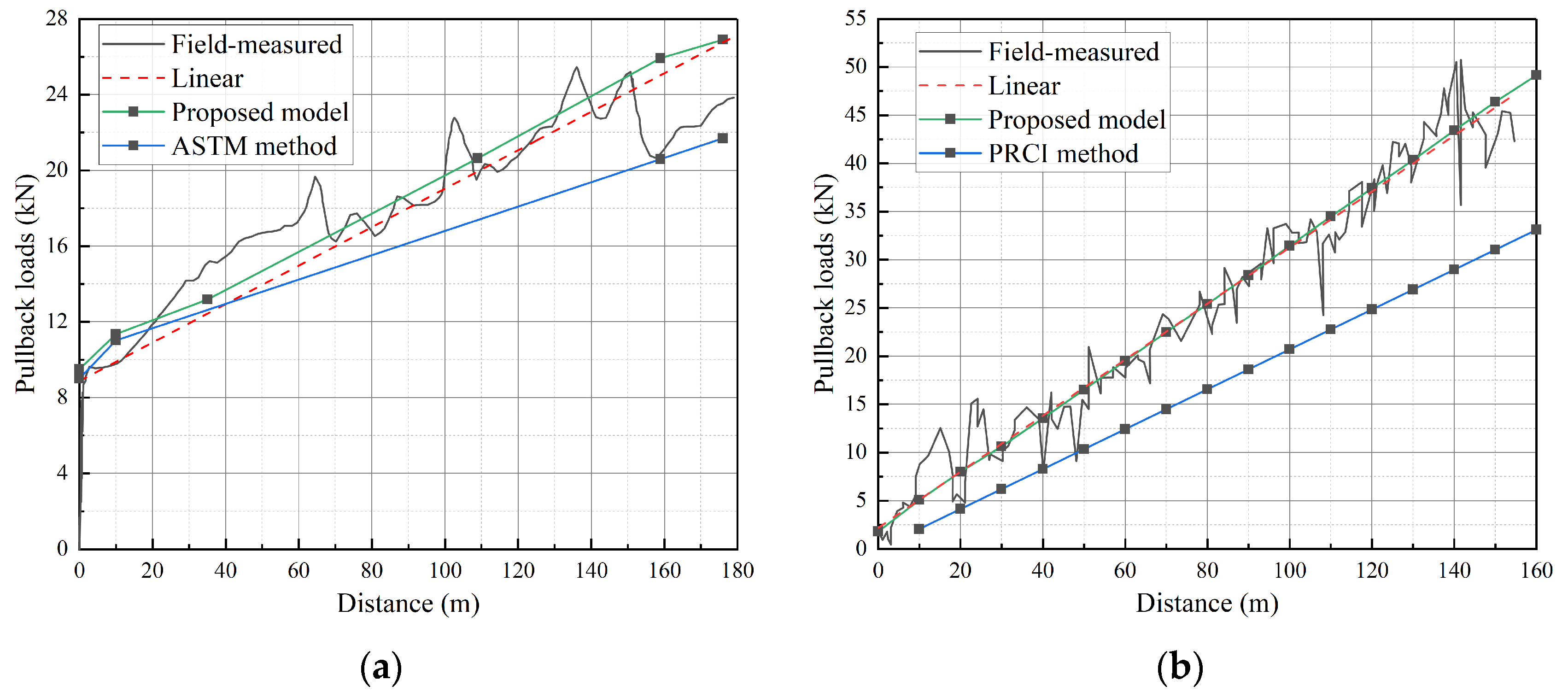
Figure 11 compares the theoretical results (including the proposed model, ASTM method, and PRCI method), field-measured results, and the linear trend line of the field-measured results for projects HD3-3 (Figure 11a) and Pull-9 (Figure 11b). Considering the applicability of existing methods, the ASTM method was used to calculate the pullback loads of project HD3-3 (HDPE pipe), and the PRCI method was used to calculate the pullback loads of project Pull 9 (steel pipe). The results are shown in Figure 11a and Figure 11b, respectively.
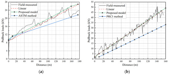
Figure 11.
Comparison between the predicted and measured values of the pipe pullback loads: (a) HD3-3, HDPE pipe; (b) Pull 9, steel pipe.
As depicted in Figure 11, the spikes in the field-measured results reflected the pullback process, which consisted of a series of pullback and stopping (disassembly of drill rods) operations. Because the analysis assumed a continuous pullback process, the trend lines of the measured results were better suited for comparison with the theoretical results [5]. It can be seen that compared to existing methods, the calculation results of the proposed model are closer to the measured results. Moreover, the rates of change of the trend lines and calculated curves were similar. The minimum and maximum relative errors between the trend line of the measured results and the proposed model for project HD3-3 (HDPE pipe) are 0.54% and 13.01%, respectively. For project Pull-9 (steel pipe), the minimum and maximum relative errors between the trend line of the measured results and the proposed model are 0.26% and 1.24%, respectively. The calculation results of the proposed model for the HDPE and steel pipes indicate that the proposed model has broader applicability. This is because the pipe–borehole wall friction force in the proposed model is based on the pipe–borehole wall contact model rather than the prescribed friction coefficient, which is not limited by the type of pipe used.
Several factors may have contributed to the differences between the theoretical and field-measured results. The first condition was that the resistance resulted from the pressure difference force at the front of the reamer. A lack of sufficient data makes it challenging to implement reasonable values in the model [46]. In the second condition, a series of recording points approximated the borehole used for the calculation. An approximate may differ from an actual borepath. The third condition was that specific material parameters used for the analysis (such as the elastic modulus, cohesion, and pressure distribution exponent n) were approximate, and even small changes in their values could affect the calculation results. Otherwise, the model provides a reasonable and widely applicable method for calculating pullback loads.
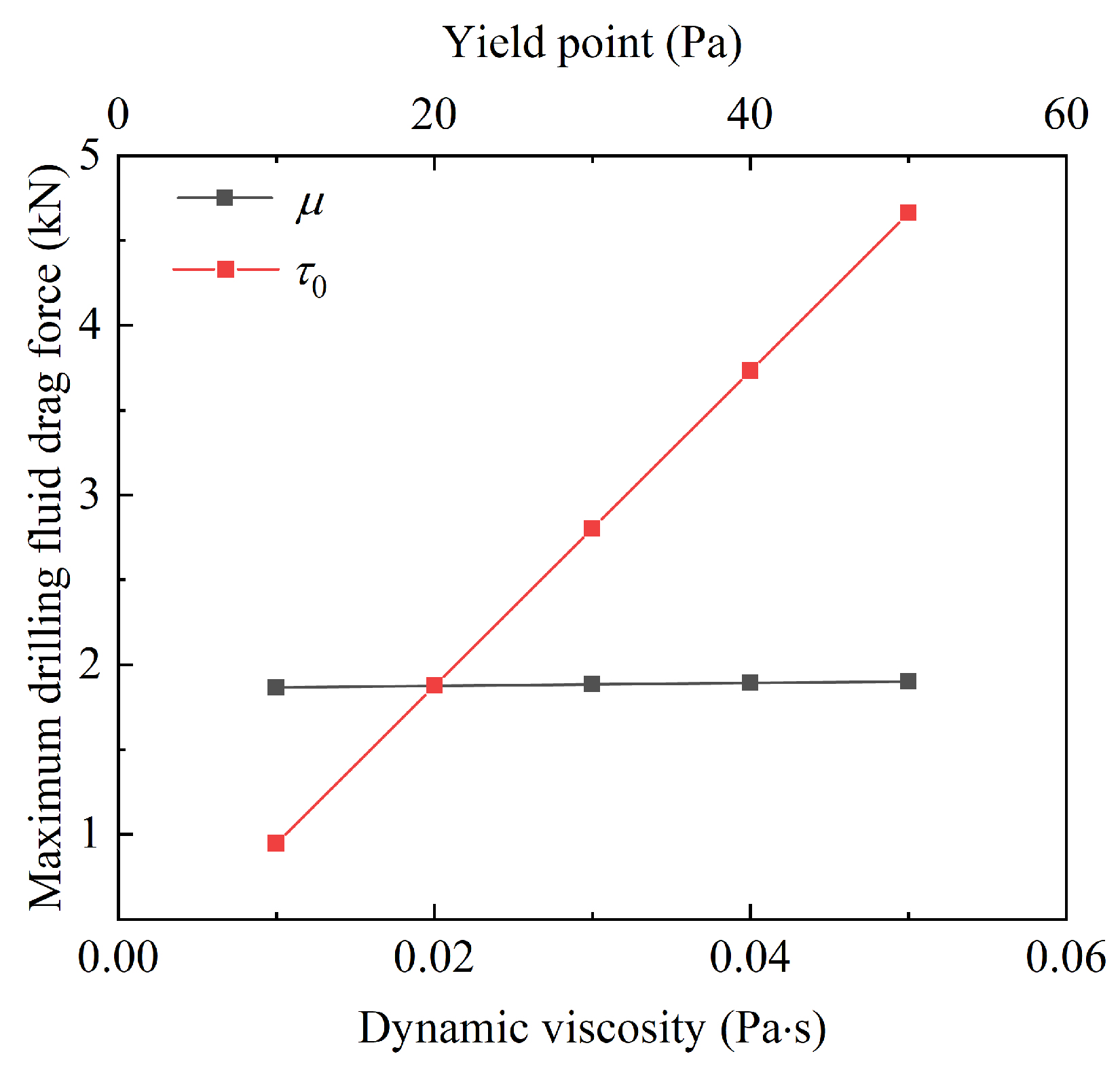
The rheological parameters τ0 and μ have a considerable influence on drilling fluid drag force. To illustrate the influence of the rheological parameters, an analysis was conducted using the HD3-3 condition. The results are shown in Figure 12. It can be seen that as τ0 and μ increase, the drilling fluid drag force also increases. However, compared to that of the yield point, the influence of viscosity on the drilling fluid drag force is minimal. This is because the shear rate of drilling fluid flow is low, and the effect of viscosity on shear stress is much smaller than that of the yield point. Moreover, the influence of temperature and time on rheological characteristics is intricate and varies based on factors such as composition and testing conditions [47,48,49]. It is essential to monitor the flow characteristics of drilling fluid in real-time during pullback operations to ensure the accuracy of the parameters used in the calculations.
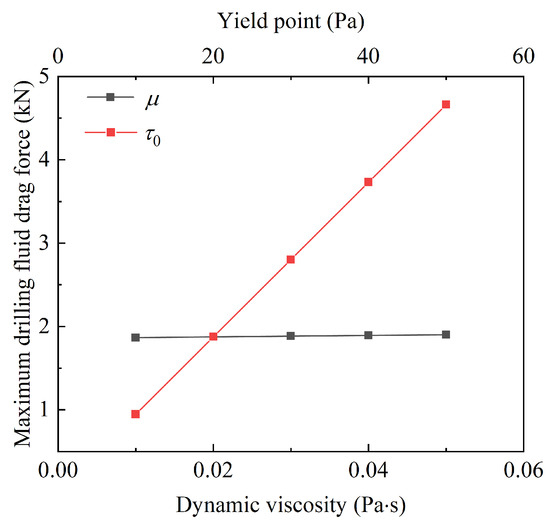
Figure 12.
Effect of rheological characteristics of drilling fluid on fluid drag force.
5. Conclusions
A method for examining pipe–borehole wall contact was presented in this paper. The contact pressure distribution and external load–displacement relationship, considering the effect of drilling fluid pressure, were derived. Compared to the Liu and Persson models, the Hertz model has the highest accuracy in calculating the maximum contact pressure when the drilling fluid pressure is not considered in HDD projects. The maximum contact pressure considering the effect of drilling fluid pressure was obtained using FEM and nonlinear regression methods. The calculation results of maximum contact pressure considering the drilling fluid pressure were very close to the FEM results, with average absolute and relative errors of 0.001 MPa and 0.6%, respectively, under the 51 test conditions. For HDD projects, the value range of the pressure distribution exponent n is generally between 0.6 and 0.75.
Additionally, based on the analysis of pipe–borehole wall contact, a novel pullback loads model was proposed. The model includes the main mechanisms that contribute to the pullback loads. The adhesion theory was used to calculate the pipe–borehole wall friction force, avoiding the influence of empirical factors on the results. The effects of the annulus size, flow rate, drilling fluid parameters, and eccentricity were considered when calculating the fluid drag force. Through case studies, the applicability and potential of the model in HDD projects were verified, and the effect of drilling fluid rheological characteristics on drilling fluid drag force was analyzed.
Notably, the variability of the construction, material, and borepath parameters will always make precise theoretical predictions of the field results challenging. A reasonable model can show the expected range of magnitudes of pipe pullback loads, variation trends of pullback loads, and influences of specific parameters on pullback loads. Thus, the proposed model exhibits good application results and prospects for HDD projects. Analysis from the contact perspective can also provide new ideas for studying pipe pullback loads.
Author Contributions
Conceptualization, Z.W. and C.H.; funding acquisition, C.H.; investigation, Z.W.; methodology, Z.W.; resources, C.H.; software, Z.W.; supervision, C.H.; validation, C.H.; writing—original draft, Z.W.; writing—review and editing, Z.W. and C.H. All authors have read and agreed to the published version of the manuscript.
Funding
This research was funded by the Key Research and Development Program of Shaanxi Province [grant number 2021SF-523], and the Natural Science Basic Research Program of Shaanxi [grant number 2022JQ-375].
Institutional Review Board Statement
Not applicable.
Informed Consent Statement
Not applicable.
Data Availability Statement
Data are contained within the article.
Conflicts of Interest
The authors declare that the research was conducted in the absence of any commercial or financial relationships that could be construed as a potential conflict of interest.
Abbreviations
| Ai (i = 1, 2 … 8) | dimensionless coefficient required to be determined/fitted |
| Ap | projected area of the pipe–borehole wall contact area |
| Ar | real contact area |
| B | function determined by n and gamma function |
| B0 | function determined by b |
| b | auxiliary variables, b = tan(ε/2) |
| C | correction factor related to the eccentricity e and the overcut ratio R2/R1 |
| c | cohesion |
| E1 | elastic modulus of the inner cylinder |
| E2 | elastic modulus of the outer cylinder |
| E* | equivalent elastic modulus |
| modified Young’s modulus of the inner cylinder | |
| e | eccentricity |
| i | number of linear calculation units before calculation point |
| k | dimensionless coefficient |
| l | semi-chord length corresponding to the angle ε |
| N | number of linear calculation units |
| n | pressure distribution exponent |
| P | external load per unit length of the pipeline |
| Pk | external load per unit length of the calculation unit k |
| p0 | maximum contact pressure accounting for the drilling fluid pressure |
| pc | contact pressure |
| q0 | maximum contact pressure without drilling fluid pressure |
| R | relative curvature of the contact |
| R1 | radius of the pipe |
| R2 | radius of the borehole |
| S | length of the pipeline entering the borehole |
| S0 | length of the pipeline at the ground |
| Sk | length of the calculation unit k |
| Ti | pullback loads for the pipeline to be pulled back to the end of calculation unit i |
| Tif | drilling fluid drag force |
| Tig | friction force between the pipeline and the ground or roller |
| Tis | friction force between the pipeline and the borehole wall |
| Tiw | pipeline’s weight |
| Tk−1 | pullback loads for the pipeline to be pulled back to the end of calculation unit k − 1 |
| Ts | Pipe–borehole wall friction force per unit length of the pipe |
| u1 | radial displacement of the inner cylinder at the contact point |
| u2 | radial displacement of the outer cylinder at the contact point |
| v | drilling fluid flow velocity |
| v1 | Poisson’s ratio of the inner cylinder |
| v2 | Poisson’s ratio of the outer cylinder |
| w | net weight of the unit length of the pipe |
| x | distance between the point on the contact surface and the symmetry axis |
| α | real contact area ratio |
| α0 | Dundurs’s material parameters |
| β | angle at which points on the interface depart from the central line |
| β0 | Dundurs’s material parameters |
| Γ | gamma function |
| Δp | maximum contact pressure increment |
| ΔPfc | pressure difference in the concentric annulus |
| ΔPf | pressure difference in HDD borehole |
| ΔPk | external load increment caused by the capstan effect |
| ΔPsti | external load increment caused by pipeline stiffness |
| ΔR | radial clearance of the pipe and borehole, ΔR = R2 − R1 |
| δ | compressive displacement |
| δk | compressive displacement of the calculation unit k |
| ε | semi-angle of contact corresponding to the whole contact arc |
| θ0 | angle between the ground and the horizontal |
| θk | inclination angle of the calculation unit k |
| θk−1 | inclination angle of the calculation unit k − 1 |
| λ | distance between centers of pipe and borehole |
| μ | dynamic viscosity of drilling fluid |
| μa | coefficient of friction applicable at the surface before the pipe enters borehole |
| σ0 | drilling fluid pressure |
| σa | normal stress |
| τ0 | yield point |
| τf | shear strength of the borehole wall |
| τs | shear (or friction) stress to break the junction (or adhesion) |
| φ | internal friction angle |
Appendix A. FEM Simulations
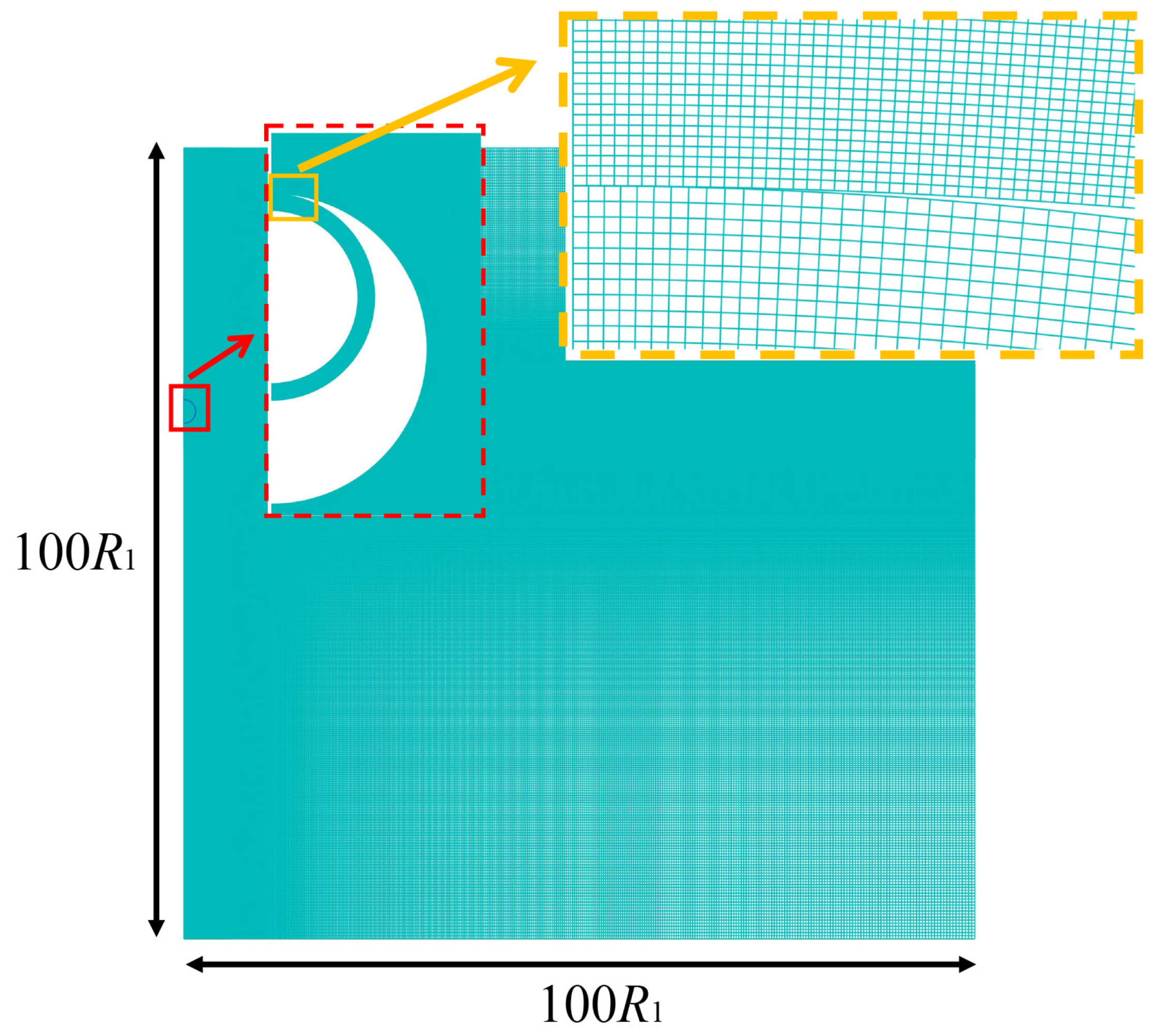
FEM simulations were performed to obtain the contact pressure distribution and external load–displacement relationship in HDD pipe–borehole wall contacts. Owing to the symmetry of the pipe and borehole, 1/2 was modeled, as shown in Figure A1. The dimensions of the borehole in the horizontal and vertical directions (W and H, respectively) were set to 100 R1 to eliminate boundary effects. The geometric and material parameters of the borehole and pipe are shown in Table 1. The bottom and right surfaces of the borehole are fixed. A symmetric boundary was applied to the middle dashed line in Figure A1. The pipe was in contact with the borehole wall under the action of 1/2 P. The borehole was subjected to drilling fluid pressure σ0. The load values are also shown in Table 1. The FEM mesh is shown in Figure A2. Element dimensions of 0.1% R1 and 0.04% R1 were tested, and the results showed negligible differences. Thus, the minimum element size was set to approximately 0.04% R1 in the FEM calculations. The FEM model was developed using the commercial software Abaqus. The analysis steps included excavation, application of drilling fluid pressure (if applicable), activation of the pipe, and application of external loads. The displacements of the pipe and borehole, as well as the contact pressure distribution, after equilibrium were used to analyze the pipe–borehole wall contact.
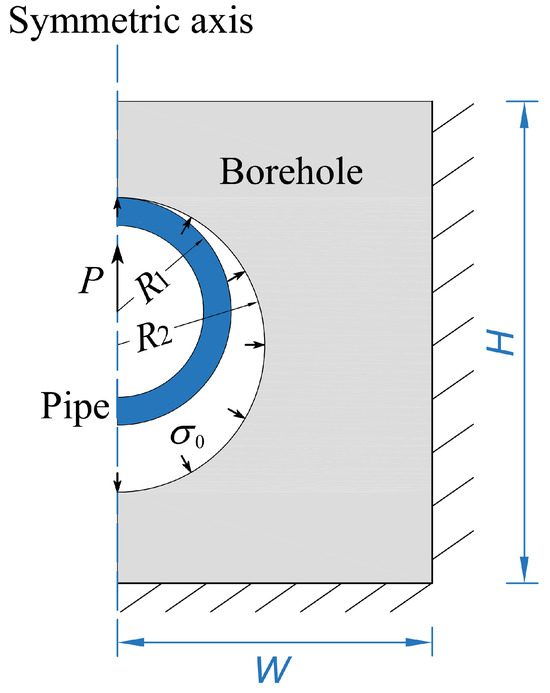
Figure A1.
FEM model for pipe–borehole wall contact.
Figure A1.
FEM model for pipe–borehole wall contact.
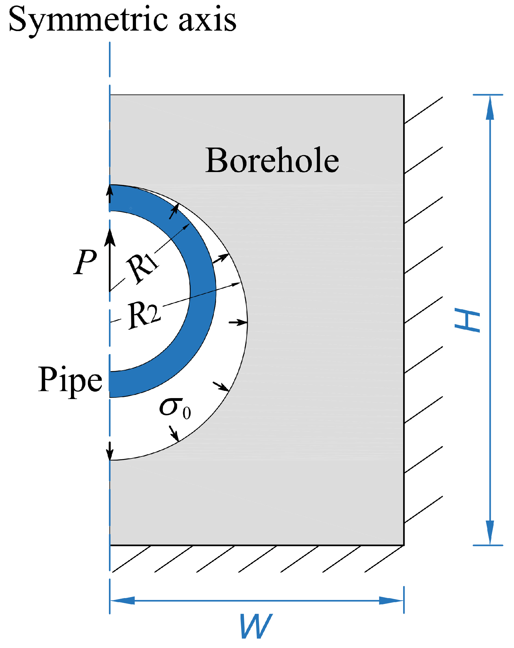
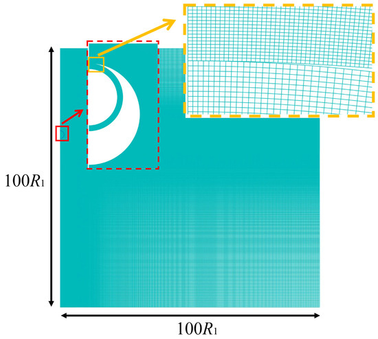
Figure A2.
FEM mesh for the simulation (element size in the contact zone is set to be 0.04%R1).
Figure A2.
FEM mesh for the simulation (element size in the contact zone is set to be 0.04%R1).
References
- Carpenter, R. HDD market growing, but challenges abound. Undergr. Constr. 2018, 73, 16–25. [Google Scholar]
- Tong, H.; Shao, Y. Mechanical Analysis of DS in Horizontal Directional Drilling. Appl. Sci. 2022, 12, 3145. [Google Scholar] [CrossRef]
- Wang, Z.Y.; Hu, C.M.; Li, L.; Yang, C.; Liang, H. Theoretical Analysis of Drilling Fluid Flow for Maxi-Horizontal Directional Drilling. J. Pipeline Syst. Eng. Pract. 2024, 15, 04024050. [Google Scholar] [CrossRef]
- Ehm, G. The changing pipeline industry. Pipes Pipelines Int. 2016, 20, 20–22. [Google Scholar]
- Polak, M.A. Analysis of polyethylene pipe behaviour in horizontal directional drilling field tests. Can. J. Civ. Eng. 2005, 32, 665–677. [Google Scholar] [CrossRef]
- Yang, C.J.; Zhu, W.D.; Zhang, W.H.; Zhu, X.H.; Ren, G.X. Determination of Pipe Pullback Loads in Horizontal Directional Drilling Using an Advanced Computational Dynamic Model. J. Eng. Mech. 2014, 140, 0401406. [Google Scholar] [CrossRef]
- Cai, L.X.; Xu, G.; Polak, M.A.; Knight, M. Horizontal directional drilling pulling forces prediction methods—A critical review. Tunn. Undergr. Space Technol. 2017, 69, 85–93. [Google Scholar] [CrossRef]
- Cheng, E.; Polak, M.A. Theoretical model for calculating pulling loads for pipes in horizontal directional drilling. Tunn. Undergr. Space Technol. 2007, 22, 633–643. [Google Scholar] [CrossRef]
- Phillips Driscopipe Company. Technical Expertise Application of Driscopipe in Directional Drilling and River Crossings; Phillips Driscopipe Company: Brownwood, TX, USA, 1993. [Google Scholar]
- Drillpath, T.M. Drillpath Theory and User’s Manual; Infrasoft LLC: Houston, TX, USA, 1996. [Google Scholar]
- ASTM F 1962-20; Standard Guide for the Use of Maxi-Horizontal Directional Drilling for Placement of Polyethylene Pipe or Conduit under Obstacles, Including River Crossings. ASTM: West Conshohocken, PA, USA, 2020.
- GB 50424-2015; Code for Construction of Oil and Gas Pipeline Crossing Project. CNPC: Beijing, China, 2015.
- Polak, M.A.; Lasheen, A. Mechanical modelling for pipes in horizontal directional drilling. Tunn. Undergr. Space Technol. 2001, 16, 47–55. [Google Scholar] [CrossRef]
- Huey, D.P.; Hair, J.D.; McLeod, K.B. Installation loading and stress analysis involvedwith pipelines installed in horizontal directional drilling. In Proceedings of the International No-Dig Conference, New Orleans, LA, USA, 31 March–3 April 1996. [Google Scholar]
- Cai, L.; Polak, M.A. A theoretical solution to predict pulling forces in horizontal directional drilling installations. Tunn. Undergr. Space Technol. 2019, 83, 313–323. [Google Scholar] [CrossRef]
- Deng, S.; Kang, C.; Bayat, A.; Kuru, E.; Osbak, M.; Barr, K.; Trovato, C. Rheological Properties of Clay-Based Drilling Fluids and Evaluation of Their Hole-Cleaning Performances in Horizontal Directional Drilling. J. Pipeline Syst. Eng. 2020, 11, 04020031. [Google Scholar] [CrossRef]
- Faghih, A.; Yi, Y.L.; Bayat, A.; Osbak, M. Fluidic Drag Estimation in Horizontal Directional Drilling Based on Flow Equations. J. Pipeline Syst. Eng. 2015, 6, 04015006. [Google Scholar] [CrossRef]
- Mulvihill, D.M.; Kartal, M.E.; Nowell, D.; Hills, D.A. An elastic–plastic asperity interaction model for sliding friction. Tribol. Int. 2011, 44, 1679–1694. [Google Scholar] [CrossRef]
- Arakawa, K. Effect of time derivative of contact area on dynamic friction. Appl. Phys. Lett. 2014, 104, 241603. [Google Scholar] [CrossRef]
- Jaber, S.B.; Hamilton, A.; Xu, Y.; Kartal, M.E.; Gadegaard, N.; Mulvihill, D.M. Friction of flat and micropatterned interfaces with nanoscale roughness. Tribol. Int. 2021, 153, 106563. [Google Scholar] [CrossRef]
- Liang, X.M.; Xing, Y.Z.; Li, L.T.; Yuan, W.K.; Wang, G.F. An experimental study on the relation between friction force and real contact area. Sci. Rep. 2021, 11, 20366. [Google Scholar] [CrossRef] [PubMed]
- Zhang, F.K.; Liu, J.H.; Ding, X.Y.; Wang, R.L. Experimental and finite element analyses of contact behaviors between non-transparent rough surfaces. J. Mech. Phys. Solids 2019, 126, 87–100. [Google Scholar] [CrossRef]
- Krick, B.A.; Vail, J.R.; Persson, B.N.J.; Sawyer, W.G. Optical in situ micro tribometer for analysis of real contact area for contact mechanics, adhesion, and sliding experiments. Tribol. Lett. 2012, 45, 185–194. [Google Scholar] [CrossRef]
- Li, L.T.; Liang, X.M.; Xing, Y.Z.; Yan, D.; Wang, G.F. Measurement of real contact area for rough metal surfaces and the distinction of contribution from elasticity and plasticity. J. Tribol. 2021, 143, 07150. [Google Scholar] [CrossRef]
- Leu, D.K. Evaluation of friction coefficient using indentation model of Brinell hardness test for sheet metal forming. J. Mech. Sci. Technol. 2011, 25, 1509–1517. [Google Scholar] [CrossRef]
- Hertz, H. On the contact of elastic solids. Reine Angew. Math. 1882, 92, 156–171. [Google Scholar] [CrossRef]
- Popov, V. Contact Mechanics and Friction, 2nd ed.; Springer: Berlin/Heidelberg, Germany, 2017. [Google Scholar]
- Persson, A. On the Stress Distribution of Cylindrical Elastic Bodies in Contact; Chalmers University of Technology: Goteborg, Sweden, 1964. [Google Scholar]
- Ciavarella, M.; Decuzzi, P. The state of stress induced by the plane frictionless cylindrical contact. I. The case of elastic similarity. Int. J. Solids Struct. 2001, 38, 4507–4523. [Google Scholar] [CrossRef]
- Ciavarella, M.; Decuzzi, P. The state of stress induced by the plane frictionless cylindrical contact. II. The general case (elastic dissimilarity). Int. J. Solids Struct. 2001, 38, 4525–4533. [Google Scholar] [CrossRef]
- Liu, C.S.; Zhang, K.; Yang, R. The FEM analysis and approximate model for cylindrical joints with clearances. Mech. Mach. Theory 2007, 42, 183–197. [Google Scholar] [CrossRef]
- Pérez-González, A.; Fenollosa-Esteve, C.; Sancho-Bru, J.L.; Sánchez-Marín, F.T.; Vergara, M.; Rodríguez-Cervantes, P.J. A modified elastic foundation contact model for application in 3D models of the prosthetic knee. Med. Eng. Phys. 2008, 30, 387–398. [Google Scholar] [CrossRef]
- Johnson, K.L. Contact Mechanics, 2nd ed.; Cambridge University Press: London, UK, 1992. [Google Scholar]
- Hu, J.Q.; Gao, F.H.; Liu, X.M.; Wei, Y.G. An elasto-plastic contact model for conformal contacts between cylinders. Proc. Inst. Mech. Eng. Part J-J. Eng. Tribol. 2020, 234, 1837–1845. [Google Scholar] [CrossRef]
- Wriggers, P. Computational Contact Mechanics; Springer: Berlin/Heidelberg, Germany, 2012. [Google Scholar]
- Aigner, L.G.; Gerstmayr, J.; Pechstein, A.S. A two-dimensional homogenized model for a pile of thin elastic sheets with frictional contact. Acta Mech. 2011, 218, 31–43. [Google Scholar] [CrossRef]
- Kamiński, M. Design sensitivity analysis for the homogenized elasticity tensor of a polymer filled with rubber particles. Int. J. Solids Struct. 2014, 51, 612–621. [Google Scholar] [CrossRef]
- Fang, X.; Yao, J.; Yin, X.; Chen, X.; Zhang, C. Physics-of-failure models of erosion wear in electrohydraulic servovalve, and erosion wear life prediction method. Mechatronics 2013, 23, 1202–1214. [Google Scholar] [CrossRef]
- Fang, X.; Zhang, C.H.; Chen, X.; Wang, Y.S.; Tan, Y.Y. A new universal approximate model for conformal contact and non-conformal contact of spherical surfaces. Acta Mech. 2015, 226, 1657–1672. [Google Scholar] [CrossRef]
- Bowden, F.P.; Tabor, D. The area of contact between stationary and between moving surfaces. Proc. R. Soc. A Math. Phys. Eng. Sci. 1939, 169, 391–413. [Google Scholar]
- Maegawa, S.; Itoigawa, F.; Nakamura, T. Effect of normal load on friction coefficient for sliding contact between rough rubber surface and rigid smooth plane. Tribol. Int. 2015, 92, 335–343. [Google Scholar] [CrossRef]
- Bourgoyne, A.T.; Millheim, K.; Chenevert, M.; Young, F.S. Applied Drilling Engineering; Society of Petroleum Engineers (SPE): Richardson, TX, USA, 1991. [Google Scholar]
- Haciislamoglu, M.; Langlinais, J. Non-Newtonian flow in eccentric annuli. J. Energy Resour. Technol. 1990, 112, 163–169. [Google Scholar] [CrossRef]
- Chehab, A.G. Time Dependent Response of Pulled-in-Place HDPE Pipes; Queen’s University: Kingston, ON, Canada, 2008. [Google Scholar]
- Baumert, M.E. Experimental Investigation of Pulling Loads and Mud Pressures during Horizontal Directional Drilling Installations; The University of Western Ontario: London, ON, Canada, 2004. [Google Scholar]
- Allouche, E.N.; Baumert, M.E. A total borehole monitoring system for pulled in place trenchless methods. In Proceedings of the International No-Dig Conference, Las Vegas, NV, USA, 31 March–2 April 2003. [Google Scholar]
- Makinde, F.A.; Adejumo, A.D.; Ako, C.T.; Efeovbokhan, V.E. Modelling the Effects of Temperature and Aging Time on the Rheological Properties of Drilling Fluids. Pet. Coal 2011, 53, 167–182. [Google Scholar]
- Ali, S.M. The Effect of High Temperature and Aging on Water-Base Drilling Fluids; King Fahd University of Petroleum & Minerals: Dhahran, Saudi Arabia, 1990. [Google Scholar]
- Santoyo, E.; Santoyo-Gutierrez, S.; García, A.; Espinosa, G.; Moya, S.L. Rheological property measurement of drilling fluids used in geothermal wells. Appl. Therm. Eng. 2001, 21, 283–302. [Google Scholar] [CrossRef]

Disclaimer/Publisher’s Note: The statements, opinions and data contained in all publications are solely those of the individual author(s) and contributor(s) and not of MDPI and/or the editor(s). MDPI and/or the editor(s) disclaim responsibility for any injury to people or property resulting from any ideas, methods, instructions or products referred to in the content. |
© 2024 by the authors. Licensee MDPI, Basel, Switzerland. This article is an open access article distributed under the terms and conditions of the Creative Commons Attribution (CC BY) license (https://creativecommons.org/licenses/by/4.0/).