Abstract
The demand for cement has significantly increased, growing by 8% in the year 2022 and by a further 12% in 2023. It is highly anticipated that this trend will continue, and it will result in significant growth by 2030. However, cement production is highly energy-intensive, with 70 to 80% of the total energy consumed during the clinker formation, which is the main cement production process. Minimising energy losses requires a radical approach that includes optimising the performance of the kilns and significantly improving their energy efficiency. One of the most efficient approaches to optimise the performance of the kilns and reduce energy losses is by integrating process re-engineering models, which leverage process data analytics, machine learning, and computational methods. This study employed a model-based integration approach to improve energy efficiency during clinker formation. Energy consumption data were collected from two semi-automated cement production plants. The data were analysed using a regression model in Minitab (Minitab 21.1.0) statistical software. The analysis resulted in a linear energy consumption equation that links energy consumption to both production and energy loss. Dynamic simulations and modelling using Simulink in MATLAB were performed based on a proportional–integral–derivative (PID)-controlled system. The dynamic behaviour of the model was evaluated using data from Plant A and validated with data from Plant B. The energy efficiency equation was established as a mathematical model that explains energy improvements based on incorporating parameters for the cement kiln system and disturbances from the environment.
1. Introduction
The cement industry is a significant contributor to global energy consumption and CO2 emissions [1], responsible for an estimated 7–8% of worldwide CO2 emissions [2]. With a current global production of 4.4 billion tons [3], both production and demand are expected to grow substantially by 2030 [1,3]. The immense energy demand of cement production, typically consuming 3.4 GJ per ton [3], highlights the urgency for innovative and sustainable alternatives to traditional cement production methods. Essentially, the conventional production of cement begins with mining, grinding raw materials into fine powders and heating the fine mixtures to form clinker [3,4]. The clinker formation process, which is the main stage in the production of cement, consumes over 70% of the total energy required [2,3,4]. Reducing energy consumption and carbon emissions during cement production is critical as it affects both the cost of production and the impact on greenhouse gas emissions. A large portion of CO2 emissions in the cement industry comes from the clinker production process, which involves heating limestone raw materials and burning fossil fuels. Addressing both energy consumption and carbon emissions in cement production is essential for safeguarding the environment, ensuring economic sustainability, and improving public health [5].
Clinker formation involves heating to calcinate a raw mix of calcium carbonate (CaCO3) and alumina–silicate materials such as clay in a rotating kiln to approximately 1450 °C [6,7,8,9,10]. This process causes the thermal breakdown of limestone, releasing carbon dioxide (CO2) and producing calcium oxide (CaO) [6]. Concurrently, the remaining oxides in the mixture undergo solid-state sintering reactions [7]. This high-temperature fusion, which inhibits full melting, promotes the formation of the main phases of tricalcium silicate (Ca3SiO5) and minor phases of dicalcium silicate (2CaO.SiO2) alongside tricalcium aluminate (3CaO.Al2O3) [8]. Essentially, the energy used to heat the raw mix to start chemical reactions usually radiates from the kilns through the kiln shell [9], amounting to 15–16% of the total energy input [10]. The hot gases also leave the kiln and carry heat energy in the form of CO2 and other combustion products. Unfortunately, around 35–39% of the total energy input is wasted during the heating process [11].
Energy consumption during clinker formation is highly dependent on the combustion system of the kiln [12], and optimising the performance of the kiln entails reducing energy losses during clinker formation [11,13]. The applicability and effectiveness of optimising the performance of the kiln vary between different kilns depending on several factors, such as kiln design and type, technology and equipment, operational practices, availability of alternative fuels, and the cost of modifications relative to the potential savings from reduced energy consumption [13]. One of the effective strategies for reducing energy losses for kilns is predictive maintenance, essentially done by adding extra sealing and insulation to the kilns and using superior refractory materials in the kiln lining [14]. Equally, other strategies for reducing energy losses for real-time kiln operations involve integrating complex control systems, such as implementing waste heat recovery systems to capture and reuse heat from the kiln’s exhaust or using advanced process control (APC) systems, which predict the performance of the kiln and make adjustments in real time to optimise fuel consumption and clinker quality [15,16]. Furthermore, energy improvement strategies for the kilns also involve employing model-based algorithms that can learn and predict changes to processes and materials to enhance energy optimisation [17,18].
Optimisation of energy consumption for cement production, using a model-based approach, can improve kiln performance and reduce energy losses [19]. The data-based approach usually involves the use of data analytics, machine learning, and other computational methods that establish process predictions and improvement scenarios for various processes involved in clinker production [19,20,21]. Some studies [20,21,22,23,24] have also suggested that model-based optimisation techniques offer a holistic and data-driven methodology for analysing energy consumption and improving energy efficiency in cement production [20]. Further, integrating process modelling with advanced controls, and predictive algorithms is one of the most feasible techniques to optimise energy-intensive operations, such as kiln heating, grinding, and clinker formation [21,22]. Additionally, leveraging real-time data and sensor technologies enables the development of dynamic models that adapt to evolving production conditions and variables [23]. These models can provide insights into the energy performance of the system, identify areas of inefficiency, and suggest optimal operating conditions [24].
Recent advances in research to improve energy efficiency have focused on integrating model-based approaches with sustainable methods to strike a balance between improving plant performance regarding energy consumption and lessening environmental effects [25]. These sustainable approaches include the use of alternative fuels such as biomass to potentially lower carbon emissions [26], together with advanced technologies that involve optimising equipment performance [26,27]. Other sustainable methods that have been studied include the use of cement blends in raw materials and feeds to reduce the carbon footprint of cement manufacturing [28]. Furthermore, the utilisation of waste materials as fuel sources, such as municipal solid waste and tire-derived gasoline, is being studied for its potential to reduce environmental impact [29].
Mathematical modelling has also played an essential role in optimising production and energy consumption for the cement industry for several decades, with regression analysis mostly used in model formulation due to its capability to identify correlations between multiple variables [30]. A fundamental regression equation usually connects a dependent variable, such as energy consumption, to one or more independent variables relevant to production [31,32]. This type of analysis has proven beneficial in predictive analytics and process optimisation, enabling producers to turn large amounts of operational data into usable information [33]. Regression models also help in understanding how numerous parameters, such as kiln temperature and raw material properties, influence energy consumption, and this allows for focused interventions to improve efficiency. The ability to predict outcomes based on current and historical data using regression modelling is one of its unique advantages that promotes successful planning and decision-making, which is imperative for improving energy efficiency [34].
The use of other modern control techniques, such as PID controllers, in cement production helps in improving energy efficiency [35]. PID controllers use feedback techniques to reduce the difference between desired and actual output values. Control signals are generated efficiently by taking into account past, present, and anticipated errors [36]. Modified PID controllers have shown great potential for optimising cement plant processes, specifically improving energy efficiency [37]. The advantages of using advanced approaches with optimised and modified PID controllers include managing the nonlinear, multi-variable dynamics and process restrictions in cement plants [37,38]. Model simulation of dynamic systems is also one of the advanced approaches that have been used in energy control systems to minimise energy use, boost efficiency, and reduce environmental pollutants while maintaining production standards [36,39]. Implementing an integrated systems approach to energy optimisation in cement plants can result in significant cost reductions [39,40].
Despite extensive research that has been conducted [12,13,14,15,16,17,18,19,20,21,22,23,24], on the use of model-based approaches to optimise energy consumption in cement production, there is still a considerable gap in knowledge on the systematic establishment of an energy consumption model in the context of clinker production, which explicitly links the optimisation of energy consumption to specific improvement strategies. Furthermore, while some studies [25,26,27,28,29,30,31,32,33,34,35,36,37,38,39,40] have also explained the potential of leveraging advanced analytics and machine learning for process optimisation, there remains a gap in developing models that continuously learn and adapt to new data, providing real-time, actionable insights and improvement strategies. The importance and urgency of the study in the current field of cement production is to address the ever-increasing challenges of climate change, the energy crisis, cost of production, and the need to reduce greenhouse gas emissions [36]. The objective of this study is to develop a model that explains energy efficiency improvements during clinker production by incorporating energy-intensive parameters of the cement kiln system. The model quantifies the heat loss caused by each parameter and its impact on the overall kiln system.
Two semi-automated cement production facilities in Zambia, known as Plant A and Plant B, provided the production and process data needed for a complete analysis under a range of production schedules and operating conditions. The strategy was to first determine the important energy-intensive parameters as a function of energy consumption from two semi-automated cement plants. The relationship between clinker production and energy consumption was determined using the regression model. A PID-controlled kiln system was established using Simulink software, producing a dynamic model that can adjust to production conditions in real time, offer useful insights, and suggest the best operational plans.
2. Materials and Methods
This section describes the approach used for data collection and pre-analysis of the data collected. Further, this section explains the concept and procedure used in developing the model and predicting energy consumption in cement production, specifically for the kiln during clinker production.
2.1. Data Collection and Pre-Analysis
The overall approach used to collect important data was to ensure that energy consumption data from cement plants were well pre-assessed and screened with reference to the total energy consumed for each plant. The input energy data were well understood in order to provide accurate insights into energy consumption and efficiency. Therefore, energy consumption data were collected from two semi-automated cement production plants in Zambia.
Production data from Plant A was collected from August 2022 to July 2023, as indicated in Table 1. The table shows the energy consumption for both electricity usage and fuel consumption, totalling 13,900.66 MJ, with an average of 1158.39 MJ per month. The overall clinker output for the year was 512,138 tons, with an average monthly production of 42,678 tons. The total cement production was 632,664 tons, with an average monthly production of 52,722 tons.

Table 1.
Production data for Plant A collected over a period of 1 year.
The production from Plant B, as shown in Table 2, was collected from April 2023 to March 2024, presenting the total energy consumed and the amounts of clinker and cement produced. Over this period, Plant B consumed a total of 1425.96 MJ, averaging 1188.3 MJ per month. Clinker production totalled 145,479 tons, with an average monthly production of 12,123.25 tons, while cement production amounted to 206,861 tons, averaging 17,238.42 tons per month. The data reflect consistent energy consumption and production rates throughout the year.
Table 2.
Production data for Plant B collected over a period of 1 year.
2.2. Selection of Energy-Intensive Parameters
In cement production, choosing the appropriate data is essential for understanding and optimising energy consumption, especially in the clinker production stage. To do this, data from two cement plants, known as Plant A and Plant B, were thoroughly investigated. During the selection stage, key variables influencing the consumption of energy were identified, and their relative importance was determined using a Pareto chart. Various operational parameters related to energy loss were collected from both plants, such as process temperatures, leakage rates, and other factors influencing energy efficiency. Table 3 provides more information on these specific factors. A Pareto chart was used to identify the variables that had the most effect on the consumption of energy. This statistical tool helps to prioritise factors by displaying the relative impact of each variable on the total energy loss.
Table 3.
Factors contributing to energy losses in clinker production.
2.3. Model Formulation
This section describes how process modelling and simulation of the PID-controlled system for regulating the temperature of a cement kiln were conducted. It highlights how feedback loops, heat loss dynamics, and PID control were employed to maintain optimal kiln temperature to ensure efficient operation. The section also highlights the use of Simulink to represent the components of the system and their simulated dynamic responses.
Modelling of Kiln System
The kiln system was modelled using MATLAB 2024a and Simulink 10.7. The primary objective was to maintain the kiln temperature at 1450 °C, which is the optimal level for clinker production. The model incorporated a feedback loop that continuously monitored the actual temperature from the plant and accounted for heat loss dynamics, ensuring stable kiln operation. As shown in Equation (1), the model was built on the basis of using a proportional–integral–derivative (PID) controller to control the kiln. The PID controller is composed of proportional, integral, and derivative components. The equation describes the ability of the PID controller to adjust the heat input of the kiln based on the real-time error, therefore managing temperature fluctuations, responding quickly to disturbances and enhancing both process stability and energy efficiency [35,36,37].
where Kp is the proportional gain, Ki is the integral gain, Kd is the derivative gain, and e(t) is the error at time t.
Transfer functions were used to simulate the dynamic responses of the burner and kiln, while heat loss to the environment was included as a major factor affecting energy efficiency. As shown in Figure 1, the model includes a total heat detector to monitor both generated and lost heat and a controlled heat detector to track heat regulated by the PID controller. Operating in a closed-loop mode, the PID controller continuously adjusts to minimise error and maintain the desired kiln temperature [37].
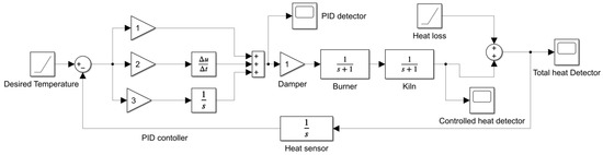
Figure 1.
Simulink model of the kiln system under PID control.
Several assumptions were made to simplify the analysis and calculations for the modelling of the kiln system. The specific heat of the reaction was assumed to be constant and independent of temperature along the axial direction. Similarly, shift and diffusion coefficients were considered independent of temperature. The damper was considered constant, as only the valve controls flow. The thermal conductivity of the refractory lining of the kilns was assumed to be 0.74 W/m/°C, the metallic wall’s conductivity was assumed to match that of alloyed carbon steel at 45 W/m/°C, and the thermal capacitance of the kiln was assumed to be 26.17 kWh/°C. The heating zone for kilns in both Plants A and B was assumed to be at 1450 °C, with the clinker density at this temperature being 1415 kg/m3. The kiln length from Plant A is 70 m and 62.5 m for Plant B.
- i.
- Convection Heat Transfer for the burner
The heat transfer between the burner and the metal surface of the kiln was calculated using the principle of energy conservation shown in Equation (2).
where is the inlet temperature, is the outlet temperature, is the density of air, V is the volume, and c is the specific heat capacity. The density of air was assumed to be 1.2 kg/m3, and the temperature of the inlet air to the burner was recorded as 26.7 °C. The volume of the burner was known to be 25 m3.
- ii.
- PID Control Mathematical Model
The mathematical model for the PID controller was considered by integrating the three controllers, the proportional controller (Kp), the integral controller (Ki), and the derivative controller (Kd). The mathematical representation of the PID controller is given in Equation (3).
where C is the controller output, Kp is the proportional constant, Kd is the derivative constant, Ki is the integral constant, and E is the error. The transfer function for the PID controller from Equation (3) is written as shown in Equation (4).
where is the control constant, and s is the Laplace function. Kp was assumed to be 1.803, Ki was assumed to be 0.08, and Kd was assumed to be 0.03 [38].
- iii.
- Convection Heat Transfer for the kiln
The heat transfer between the burner and the metal surface of the kiln was calculated using the principle of energy conservation shown in Equation (5).
where is the inlet temperature of the kiln, is the outlet temperature of the kiln, is the density of clinker at 1450 °C, V is the volume of the kiln, and c is the specific heat capacity of the kiln shell. The heat transfer through the layers of the wall of the kiln and the bulk flow of clinker was assumed to be in a steady state.
- iv.
- Mathematical model for the heat sensor
The mathematical model for the heat sensor was established as the output of the thermocouple sensor system in response to temperature changes in the system over time, as described in Equation (6).
where R is the resistance ratio given by voltage over current, τ is the time constant, and t is the time, whereas the exponential term describes how the sensor’s response decays over time.
Integrating Equation (6) gives Equation (7), and assuming the first-order system with an exponential response function, the transfer function is represented in Equation (8).
- v.
- Total heat loss
The heat lost to the environment, which is a function of the kiln’s temperature, was considered an important factor in maintaining the desired temperature of the system and was defined in Equation (9):
where Q is the total heat lost from the kiln, t is the time, h is the heat transfer coefficient, and A is the surface area through which heat is lost. is the temperature of the system, and is the ambient temperature of the environment. The transfer function for heat loss can be defined as follows:
where represents the thermal dynamics of the kiln system.
3. Results
This section presents the findings, with an emphasis on the energy loss variables and predictive models created for two cement production plants, referred to as Plant A and Plant B. Pareto charts and regression analysis are used to analyse and present the factors that influence energy consumption during clinker production. Furthermore, the relationship between clinker production and energy consumption is investigated, offering insight into potential solutions for increasing energy efficiency in these plants. The findings presented in this part provide useful insights into the primary causes of energy inefficiency in cement production, as well as actionable recommendations for improving overall energy performance.
3.1. Selection of Energy Intensive Parameters
Figure 2 shows a Pareto chart analysing the energy loss details in Plant A. The graph identifies and prioritises the factors that contribute to energy loss. The graphic indicates that the total energy loss in Plant A is 1889.07 MJ per year. The graph also shows that the most significant sources of energy loss are the flue gas temperature leaving the kiln (FgTK), clinker discharge temperature (CDT), flue gas temperature at the recovery point (FgTR), and overload flue gas temperature (OFgT). These four parameters alone account for 96% of total energy losses, as seen in Equation (11).
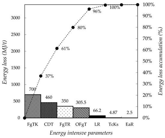
Figure 2.
Pareto chart to analyse the energy loss parameters in Plant A.
Figure 2 also highlights essential opportunities where solutions to improving energy efficiency can be most successfully applied by identifying these key factors. For example, high temperatures in the flue gases leaving the kiln indicate large heat losses, meaning that enhancing heat recovery systems or optimising kiln operation might significantly minimise these losses. Similarly, high clinker discharge temperatures suggest inefficient heat transfer processes in the kiln and cooling systems. Enhancing the efficiency of clinker cooling can result in significant energy savings. High temperatures at the flue gas recovery point indicate possible inefficiencies in heat recovery units, implying that improvements could include greater insulation, enhanced heat exchanger design, or sophisticated control systems to maximise heat recovery. The factors should be considered for model design with a direct correlation to overall energy losses for Plant A.
Figure 3 shows a Pareto chart for energy loss details in Plant B. The figure provides a clear visual representation of the numerous aspects contributing to energy losses, allowing for prioritising energy improvement measures. Figure 3 indicates that the total energy loss for Plant B is 1839.87 MJ annually. The graph shows the most significant sources of energy loss, with the tertiary air duct damper temperature (TaDT), cooler air exhaust temperature (CaET), flue gas temperature at the recovery point (FgTR), and overload flue gas temperature (OFgT) being the main contributors. These components account for 95% of total energy losses, as seen in Equation (12).
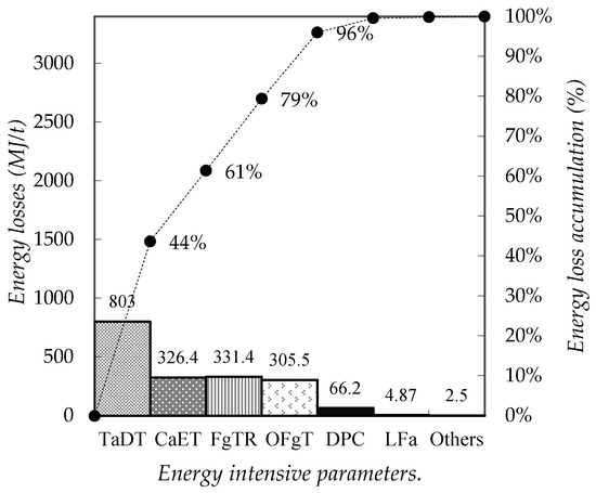
Figure 3.
Pareto chart to analyse the energy loss parameters in Plant B.
The substantial proportion of energy loss (95%) attributed to these specific factors suggests that these are important factors for designing the model that can optimise energy consumption for Plant B.
3.2. Correlation of Energy Consumption and Factors Affecting Energy Loss
Figure 4 shows the regression plot for clinker production for Plant A, which is based on a regression model that links the amount of energy consumed to clinker production. The graph compares the observed data points to their expected values. The figure shows that the R2 value of 0.749 indicates a strong linear relationship, implying that clinker production volumes account for 74.9% of the variability in energy consumption.
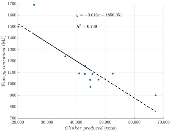
Figure 4.
Regression plot for energy consumption for clinker produced for Plant A.
Equation (13) describes the linear relationship between energy consumption and clinker production. According to this model, assuming no clinker is produced ( = 0 tons), the projected energy consumption per ton is 1850 MJ. This baseline energy consumption covers all of the plant’s fixed energy requirements.
where is the energy consumed, and represents clicker production in tons.
The regression model predicts that as clinker production increases, energy consumption per ton will decrease. This is supported by the regression equation’s negative slope coefficient (−0.016). The negative coefficient indicates that with each new ton of clinker produced, the energy consumption per ton drops significantly. This suggests that the plant becomes more energy efficient as production increases. Several factors contribute to the reduction in energy consumption with increasing tons of clinker produced. One major factor is the increased utilisation of the fixed energy requirement for the plant. When production is low, the energy required to keep the plant running (baseline energy) is distributed among fewer units, resulting in increased energy consumption per unit. As production increases, the fixed energy cost can be spread out over a larger number of units, lowering energy consumption per ton.
Figure 5 shows the regression plot for clinker production for Plant B, which is based on a regression model that links the amount of energy consumed to clinker production.
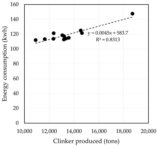
Figure 5.
Regression plot for energy consumption for clinker produced for Plant B.
The graph compares the observed data points to their expected values according to a normal distribution. The linear relation is expressed by Equation (14), which describes the relationship between energy consumption and clinker production.
where is the energy consumed, and represents clicker production in tons.
The positive slope coefficient indicates that for every one-unit increase in clinker production, the energy consumed increased by 0.0045 units. In this context, if clinker production increases, the model predicts a slight decrease in energy consumption per unit of clinker produced. This suggests a trend towards greater energy efficiency with increasing production. The intercept value (583.7) suggests the baseline energy consumption that occurs regardless of production. As clinker production increases, the model predicts a decrease in energy consumption per unit of clinker produced, as indicated by the negative slope coefficient. This relationship implies some level of energy efficiency improvement or optimisation with increasing production levels. The R2 for model fit for Plant B is 0.83.
Figure 6 shows an energy consumption order plot, which indicates the normalised residuals of energy consumption data vs. the observation order for Plant A. The line plot joins each observation’s standardised residuals, allowing for visual detection of patterns, trends, or deviations. In a well-fitted regression model, residuals should be evenly distributed around the zero line, showing non-systematic tendency. However, Figure 6 shows large variances, especially in the 4th and 12th observations, where standardised residuals exceed 2. These points could be regarded as outliers, suggesting considerable differences between the model’s predictions and actual values.
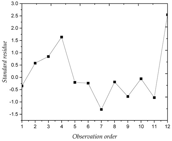
Figure 6.
Energy consumption order plot for Plant A.
Figure 7 shows an energy consumption order plot, which indicates the normalised residuals of energy consumption data vs. the observation order for Plant B.
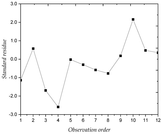
Figure 7.
Energy consumption order plot for Plant B.
As shown in Figure 7, there is a large variance, particularly at the 4th and 10th observations, where standardised residuals exceed 2. These points may be considered outliers, indicating significant discrepancies between the model’s predictions and actual values.
In Figure 8, the logarithmic energy consumption curve, along with confidence intervals for Plant A, illustrates how energy efficiency improves with higher production volumes. It also highlights how energy consumption varies across different production levels.
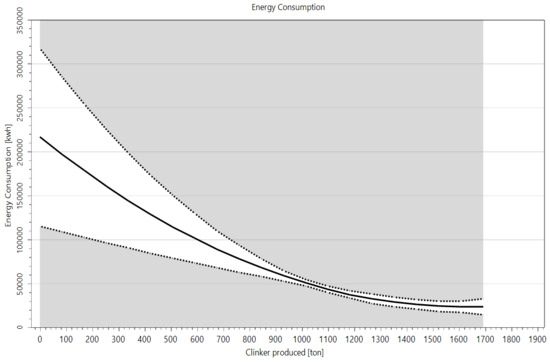
Figure 8.
Logarithmic energy consumption curve with confidence intervals for Plant A.
According to the graph, clinker production for Plant A decreases the amount of energy consumed, indicating an inverse relationship. Solid lines indicate the predicted energy consumption based on clinker production, while dotted lines represent confidence intervals, which indicate the range of actual energy consumption values that are anticipated to decrease within a specific possibility. The shaded background indicates the area covered by the confidence intervals, illustrating the range of variability around the main trend. At higher volumes, the accuracy of energy consumption projections is enhanced as the confidence intervals diminish, demonstrating improved process stability and control. In particular, the lower end of the energy consumption range at peak output emphasises the importance of high-volume production for improving efficiency.
Figure 9 also shows that energy consumption for Plant B increases as clinker production increases. Initially, the energy consumption is relatively low for lower levels of clinker production and increases as production rises. This suggests that as more clinker is produced, the process becomes more energy-efficient. The confidence intervals indicate that there is variability in energy usage, which could be caused by numerous operational or external factors, such as fluctuations in raw material quality or weather conditions. Despite this variability, the overall trend shows improvement in energy efficiency with increased clinker production.
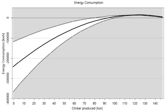
Figure 9.
Logarithmic energy consumption curve with confidence intervals for Plant B.
3.3. Kiln System Simulation
The average temperature of the gas entering the burner was 26.7 °C, the volume was 25 m3, and the density of air was 1.2 kg/m3. The system response using the equation can be solved as follows:
The transfer function of the kiln for Plant A, calculated using the actual volume of the kiln and inlet temperature, is as follows:
For Plant B, the transfer function of the kiln is as follows:
The transfer function of the heat sensor is calculated using Equation (8) and indicates the transfer function results as follows:
The transfer function of the PID is calculated using Equation (4):
The transfer function for the heat loss is calculated using Equation (2):
where is defined as , and is the heat loss to the environment.
Therefore, the closed-loop equation for the kiln system model is as follows:
The energy efficiency of the system can be defined as follows:
The improvement is established as shown in Equation (23).
Figure 10 shows a Simulink schematic of a PID-controlled system that maintains the cement kiln temperature at 1450 °C. The system determines the difference between the desired and actual temperatures, which are subsequently controlled by a PID controller with proportional, integral, and derivative components. This PID controller controls the damper to manage the airflow and fuel mixture to the burner, with a transfer function indicating the dynamic response. The thermal dynamics of the kiln are also represented by a transfer function, which specifies how it responds to heat input. In addition, the system accounts for heat loss using another transfer function. A complete heat detector measures both generated and lost heat, providing feedback to maintain accurate temperature control.
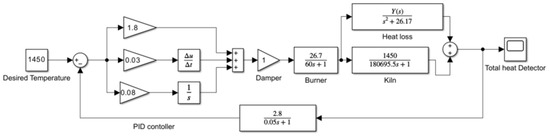
Figure 10.
Simulated kiln system model for Plant A, showing improved energy efficiency.
Figure 11 shows the dynamic response model for the burner in the cement kiln system, which is modelled using the transfer function in Equation (13) to control inputs over time. This function describes a first-order system, in which the temperature response increases exponentially towards a steady-state value. The response curve indicates that the burner output can be modified to attain the ideal kiln temperature of 1450 °C, which is required for clinker formation. The constant of time τ, obtained from the denominator of the transfer function, is 60 s, showing the time required for the system to achieve approximately 63.2% of its final value. The time constant shows small values, which indicate how fast the system responds.
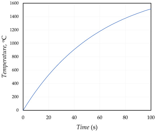
Figure 11.
Response function of the burner.
Figure 11 also indicates that the system stabilises after around 100 s without exceeding the specified temperature, proving that the PID controller is effectively tuned. The absence of overshoot and oscillations in the graph indicates that the control system provides stability and has the ability to efficiently handle process disruptions, emphasising the significance of an optimised burner response for energy efficiency.
Figure 12 presents the response function of a heat sensor in a cement kiln system. The graph indicates that the temperature immediately rises to roughly 1400 °C before stabilising at this level, suggesting that the system quickly achieves and maintains the desired temperature. The system stabilises after 2 s, which indicates that the control mechanism, likely a PID controller, is well tuned to respond swiftly and effectively. The absence of temperature overshoot in the curve suggests that the control system is highly effective in ensuring that the temperature does not exceed the desired level.
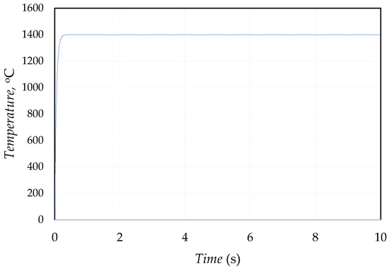
Figure 12.
Response function for the heat sensor.
Figure 13 shows the temperature response of a kiln system over time, controlled by a PID control system. The figure shows the temperature rises rapidly and exceeds the set point, but then gradually decreases and settles around the ideal temperature of 1400 °C. The system settles in approximately 40 s, indicating how long it takes the PID controller to adapt and maintain the desired temperature without oscillations. This type of response is characteristic of PID-controlled systems, designed to reach the setpoint efficiently while reducing overshoot and ensuring rapid stability. The graph shows how the control system manages kiln temperature, responds fast to changes, and achieves steady-state conditions. This results in high efficiency and consistent product quality, demonstrating a powerful control system that meets contemporary cement production standards.
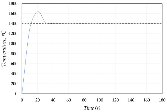
Figure 13.
Response function for the PID-controlled system of the kiln for Plant A.
The graph in Figure 14 presents the temperature response for a PID-controlled and non-controlled system in Plant B. The PID-controlled system initially reaches a peak temperature before settling to a stable temperature of approximately 1200 °C. This mirrors the actions of the PID controller, which responds quickly to reduce error and stabilise the system. The system without control has a significant overrun, reaching temperatures above the desired setpoint. It exhibits more noticeable oscillations, indicating a lack of control and difficulty in stabilising quickly. The graph validates the model’s behaviour by showing that the model for Plant A matches the effective control dynamics provided by the PID system in Plant B, proving its precision and applicability.
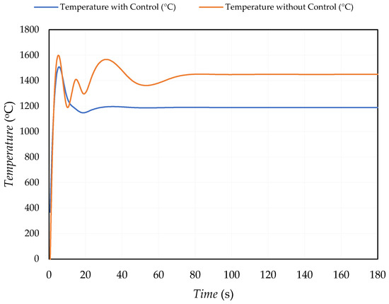
Figure 14.
Response function for the kiln system for Plant B.
4. Discussion
According to the data collected and analysed, the annual energy loss for Plant A accumulates to 1889.07 MJ. The four major factors that contribute to this energy loss are overload flue gas temperature (OFgT), clinker discharge temperature (CDT), recovery point flue gas temperature (FgTR), and flue gas temperature (FgTK). Pareto analysis indicates that these four variables account for 96% of all energy losses. A significant reduction in energy loss could be achieved by implementing improvement strategies that are related to these four variables. The improvement strategies must include insulation and heat recovery. In recent studies [41,42,43] and other studies [44,45,46,47], it has been shown that optimising heat recovery systems and improving insulation are effective strategies for improving energy efficiency in industrial processes. Therefore, by focusing on these areas, Plant A can significantly reduce its energy consumption and align with best practices in cement manufacturing energy management. Regression analysis for Plant A indicates that there is a significant relationship (R2 = 0.749) between clinker production and energy consumption. The analysis indicates that energy consumption per ton reduces with increasing production volume. This is because fixed energy costs are distributed across higher production volumes, indicating substantial efficiencies in production.
Plant B, on the other hand, has an annual energy loss of 1856.5 MJ, with a different set of causes. The tertiary air duct damper temperature (TaDT), cooler air exhaust temperature (CaET), flue gas temperature at the recovery point (FgTR), and overload flue gas temperature (OFgT) all contribute significantly to energy losses, accounting for 95% of the total. Plant B has different production and energy consumption trends compared to Plant A. The regression model shows a stronger association (R2 = 0.83) between energy usage and clinker production. This implies that Plant B benefits from a lower drop in energy consumption per unit produced, indicating different operational constraints or efficiency compared to Plant A. The variations in operational efficiency could be attributed to differences in equipment, process technology, or operational methods. Using Pareto analysis, Plants A and B can identify solutions tailored to their specific energy challenges and prioritise them accordingly.
The dynamic simulations of the cement kiln system using Simulink indicate that the use of a PID-controlled system is effective at managing kiln temperature and maintaining process stability. The burner and kiln transfer functions define how well the system responds to input changes, resulting in a quick temperature rise to the desired setpoint with little overshoot. This rapid stabilisation within a short timeframe indicates that the PID controller is precise and effective in minimising fluctuations and maintaining steady-state conditions, as supported by studies [48,49,50]. The PID controller helps optimise energy usage by minimising temperature variations, which has been highlighted in the literature as an important component in improving system sustainability [50]. The rapid stabilisation is consistent with research findings [51,52], which indicate that well-tuned PID systems can greatly enhance energy efficiency, adding to the sustainability goals emphasised in current research. Furthermore, the absence of significant fluctuations and overshoot in the response of the system demonstrates precision in achieving desired operating conditions. This level of control indicates that the model is both energy-efficient and capable of delivering consistent controls required for product quality. These findings are consistent with previous research [48,49,50,51], which emphasises the importance of rigorous control strategies in cement manufacturing to preserve product quality while optimising energy use.
The energy efficiency equation expressed in Equation (21) provides a metric for determining the energy efficiency of a cement kiln system over a certain time. This equation emphasises the magnitude of the closed-loop transfer function, which describes the dynamic reaction of the system to inputs and disturbances while ensuring stable functioning. By integrating this response over time, the equation gives useful information on the effectiveness of the PID controllers, specifically its capacity to reduce temperature fluctuations and stabilise the system. For Plant A, where considerable energy losses are caused by factors such as high flue gas and clinker discharge temperatures, reaching a higher energy efficiency measure requires effective control over these parameters. This can lead to less energy waste and more operational efficiency. Similarly, in Plant B, where air duct and cooler exhaust temperatures are the key sources of energy loss, an elevated measure of energy efficiency would indicate first-rate management of these inefficiencies. This can ensure the kiln operates under optimal circumstances for clinker formation. By comparing the dynamic behaviour of Plant A and Plant B, the model for Plant A can be validated against the observed performance in Plant B, indicating that PID control effectively captures the required control dynamics. This comparison demonstrates that the model accurately reproduces real-world behaviour, demonstrating its precision and suitability for predicting and optimising kiln operations under identical conditions.
In both plants, optimising the PID control system to improve energy efficiency not only contributes to energy saving but also supports sustainable cement production by lowering the carbon footprint and operational expenses associated with excessive energy consumption. As a result, the established energy efficiency equation incorporates the identified areas for improvement as a function of heat loss and ensures that both plants waste as little energy as possible, in line with industry sustainability and cost-effectiveness standards.
5. Conclusions
Factors affecting energy efficiency were identified from the collected production data from two semi-automated plants. The analysis of Plants A and B revealed that high energy losses at Plant A are related to high flue gas temperatures and clinker discharge temperatures, which accounted for 96% of energy inefficiencies. The energy losses for Plant B were related to issues such as the tertiary air duct damper temperature, cooler air exhaust temperature, and other related factors, which account for 95% of total losses.
The regression analysis for Plant A established a strong correlation between energy consumption and clinker production, emphasising the advantages of higher production efficiency because of lower energy consumption per unit of clinker produced. The regression model for Plant B established an even stronger relationship between energy consumption and production, indicating that further improvements in techniques can greatly increase energy efficiency.
The dynamic behaviour of the PID-controlled system showed a rapid stabilisation of kiln temperature, quickly reaching the desired setpoint with minimal overshoot. The system effectively minimised fluctuations, maintaining steady-state conditions with precise control, contributing to improving energy efficiency. The absence of significant overshoot further confirmed the accuracy of the system in achieving the desired operating conditions. This stable and efficient performance ensured consistent process stability, essential for maintaining product quality in cement manufacturing.
The energy efficiency equation was developed as a mathematical model that incorporates heat loss to the environment as a system disturbance. This model captures the dynamic response of the system by focusing on the closed-loop transfer function, which is critical for maintaining steady operation. This approach simulates real-world energy losses and disturbances and indicates that the established model adapts to the dynamic operational requirements of processes like cement production, where maintaining stability and efficiency despite varying conditions is essential.
Author Contributions
Conceptualisation, M.C.S.; methodology, M.C.S.; software, W.E.; formal analysis, T.Z.; data curation, W.E.; writing—original draft preparation, M.C.S.; writing—review and editing, T.Z.; visualisation, M.C.S.; supervision, E.L., I.N.S. and T.Z.; project administration, E.L. All authors have read and agreed to the published version of the manuscript.
Funding
This research received no external funding.
Institutional Review Board Statement
The study was conducted in accordance with the guidelines of the University of Zambia’s Directorate of Research and Graduate Studies (30 March 2023), Natural and Applied Sciences Research Ethics Committee.
Informed Consent Statement
Not applicable.
Data Availability Statement
The raw data supporting the conclusions of this article will be made available by the corresponding author on request.
Acknowledgments
We extend our sincere appreciation to the academic team of the Department of Agriculture, School of Engineering, University of Zambia, for their guidance throughout the research.
Conflicts of Interest
The authors declare no conflicts of interest.
References
- International Energy Agency. World Energy Outlook 2020; IEA Licence: Creative Commons Attribution CC BY-NC-SA 4.0. 2020. Available online: https://www.iea.org/energy-system/industry/cement (accessed on 13 June 2024).
- Ighalo, J.O.; Adeniyi, A.G. A perspective on environmental sustainability in the cement industry. Waste Dispos. Sustain. Energy 2020, 2, 161–164. [Google Scholar] [CrossRef]
- Verma, Y.K.; Mazumdar, B.; Ghosh, P. Thermal energy consumption and its conservation for a cement production unit. Environ. Eng. Res. 2020, 26, 200111. [Google Scholar]
- Hasanbeigi, A.; Price, L.; Lin, E. Emerging Energy-Efficiency and CO2 Emission-Reduction Technologies for Cement and Concrete Production: A Technical Review. Renew. Sustain. Energy Rev. 2012, 16, 6220–6238. [Google Scholar] [CrossRef]
- Akintayo, B.D.; Akintayo, D.C.; Olanrewaju, O.A. Material Substitution Strategies for Energy Reduction and Greenhouse Gas Emission in Cement Manufacturing. Atmosphere 2023, 14, 1200. [Google Scholar] [CrossRef]
- Sousa, V.; Bogas, J.A. Comparison of energy consumption and carbon emissions from clinker and recycled cement production. J. Clean. Prod. 2021, 306, 127277. [Google Scholar] [CrossRef]
- Antunes, M.; Santos, R.L.; Pereira, J.; Rocha, P.; Horta, R.B.; Colaço, R. Alternative Clinker Technologies for Reducing Carbon Emissions in Cement Industry: A Critical Review. Materials 2021, 15, 209. [Google Scholar] [CrossRef] [PubMed] [PubMed Central]
- Andrew, R.M. Global CO2 Emissions from Cement Production, 1928–2018. Earth Syst. Sci. Data 2019, 11, 1675–1710. [Google Scholar] [CrossRef]
- Wang, Y.; Cui, S.; Lan, M.; Tian, G.; Liu, L. Influence of characteristics of alumina-silicate raw materials on the formation process of clinker. J. Wuhan Univ. Technol.-Mater. Sci. Ed. 2014, 29, 966–971. [Google Scholar] [CrossRef]
- Laita, E.; Bauluz, B.; Yuste, A. High-Temperature Mineral Phases Generated in Natural Clinkers by Spontaneous Combustion of Coal. Minerals 2019, 9, 213. [Google Scholar] [CrossRef]
- Alemayehu, F.; Sahu, O. Minimization of Variation in Clinker Quality. Adv. Mater. 2013, 2, 23. [Google Scholar] [CrossRef]
- Onwukwe, J.C.; Ugonabo, V.I. Optimization of Heat Consumption in a Rotary Cement Kiln. Int. J. Latest Technol. Eng. Manag. Appl. Sci. 2019, 8, 95–101. [Google Scholar]
- Zanoli, S.M.; Pepe, C.; Rocchi, M. Control and optimisation of a cement rotary kiln: A model predictive control approach. In Proceedings of the 2016 Indian Control Conference (ICC), Hyderabad, India, 4–6 January 2016; pp. 111–116. [Google Scholar]
- Titov, O.V.; Beloglazov, I.I. Effectiveness of Different Designs of Refractory Linings for Rotary Kilns in Relation to Their Thermophysical Properties. Refract. Ind. Ceram. 2015, 56, 260–262. [Google Scholar] [CrossRef]
- Parks, L.; Sherwen, R. The use of new materials in an improved design of rotary kiln. Mater. Des. 1986, 7, 252–255. [Google Scholar] [CrossRef]
- Zanoli, S.M.; Pepe, C.; Astolfi, G. Advanced Process Control for Clinker Rotary Kiln and Grate Cooler. Sensors 2023, 23, 2805. [Google Scholar] [CrossRef]
- Mujumdar, K.S.; Arora, A.; Ranade, V.V. Modeling of Rotary Cement Kilns: Applications to Reduction in Energy Consumption. Ind. Eng. Chem. Res. 2006, 45, 2315–2330. [Google Scholar] [CrossRef]
- Ryan, J.; Bussmann, M.; DeMartini, N. CFD Modelling of Calcination in a Rotary Lime Kiln. Processes 2022, 10, 1516. [Google Scholar] [CrossRef]
- El-Salamony, A.-H.R.; Mahmoud, H.M.; Shehata, N. Enhancing the efficiency of a cement plant kiln using modified alternative fuel. Environ. Nanotechnol. Monit. Manag. 2020, 14, 100310. [Google Scholar] [CrossRef]
- Sismanis, P. Prediction of Productivity and Energy Consumption in a Consteel Furnace Using Data-Science Models. In Business Information Systems; Springer: Cham, Switzerland, 2019. [Google Scholar]
- Oguntola, O.; Boakye, K.; Simske, S. Towards Leveraging Artificial Intelligence for Sustainable Cement Manufacturing: A Systematic Review of AI Applications in Electrical Energy Consumption Optimization. Sustainability 2024, 16, 4798. [Google Scholar] [CrossRef]
- Lorimer, D.M.; Murray, P. Industrial strategies to help reduce energy consumption: A holistic approach for cement producers. In Proceedings of the 2010 IEEE-IAS/PCA 52nd Cement Industry Technical Conference, Colorado Springs, CO, USA, 28 March–1 April 2010; pp. 1–7. [Google Scholar]
- Swanepoel, J.A.; Mathews, E.H.; Vosloo, J.; Liebenberg, L. Integrated energy optimisation for the cement industry: A case study perspective. Energy Convers. Manag. 2014, 78, 765–775. [Google Scholar] [CrossRef]
- Chatzilenas, C.; Gentimis, T.; Dalamagas, T.; Kokossis, A.C.; Katsiaboulas, A.; Marinos, I. Machine learning applications and process intelligence for cement industries. In Proceedings of the 31st European Symposium on Computer Aided Process Engineering, Istanbul, Turkey, 6–9 June 2021. [Google Scholar]
- Naranje, V.; Chidambaram, T.V.S.; Garg, R.B.; Bachchhav, B.D. Use of Sustainable Practices in Cement Production Industry: A Case Study. In Advances in Manufacturing Systems; Kumar, S., Rajurkar, K.P., Eds.; Lecture Notes in Mechanical Engineering; Springer: Singapore, 2021. [Google Scholar] [CrossRef]
- Saleh, E.-D.M. Cement Industry—Optimisation, Characterisation and Sustainable Application; IntechOpen: London, UK, 2021. [Google Scholar] [CrossRef]
- Cantini, A.; Leoni, L.; De Carlo, F.; Salvio, M.; Martini, C.; Martini, F. Technological Energy Efficiency Improvements in Cement Industries. Sustainability 2021, 13, 3810. [Google Scholar] [CrossRef]
- Sahoo, N.; Kumar, A.; Samsher. Review on Energy Conservation and Emission Reduction Approaches for Cement Industry. Environ. Dev. 2022, 44, 100767. [Google Scholar] [CrossRef]
- Adesina, A.; Awoyera, P. Utilisation of Biomass Energy in Cement Production: A Pathway Towards Sustainable Infrastructure. In Renewable Energy and Sustainable Buildings; Sayigh, A., Ed.; Innovative Renewable Energy; Springer: Cham, Switzerland, 2020. [Google Scholar] [CrossRef]
- Maekawa, K.; Ishida, T.; Kishi, T. Multi-Scale Modeling of Concrete Performance. J. Adv. Concr. Technol. 2003, 1, 91–126. [Google Scholar] [CrossRef]
- Goshayeshi, H.R.; Poor, F.K. Modeling of Rotary Kiln in Cement Industry. Energy Power Eng. 2016, 8, 23–33. [Google Scholar] [CrossRef]
- Stadler, K.S.; Poland, J.; Gallestey, E. Model predictive control of a rotary cement kiln. Control Eng. Pract. 2011, 19, 1–9. [Google Scholar] [CrossRef]
- Tahmasebinia, F.; Jiang, R.; Sepasgozar, S.; Wei, J.; Ding, Y.; Ma, H. Using Regression Model to Develop Green Building Energy Simulation by BIM Tools. Sustainability 2022, 14, 6262. [Google Scholar] [CrossRef]
- Fellaou, S.; Harnoune, A.; Seghra, M.A.; Bounahmidi, T. Statistical Modeling and Optimization of the Combustion Efficiency in Cement Kiln Precalciner. Energy 2018, 155, 351–359. [Google Scholar] [CrossRef]
- Swanepoel, J.A. Modelling for integrated energy optimisation in cement production. In Proceedings of the 10th Industrial and Commercial Use of Energy Conference, Cape Town, South Africa, 20–21 August 2013; pp. 1–6. [Google Scholar]
- Barbhuiya, S.; Kanavaris, F.; Das, B.B.; Idrees, M. Decarbonising Cement and Concrete Production: Strategies, Challenges and Pathways for Sustainable Development. J. Build. Eng. 2024, 86, 108861. [Google Scholar] [CrossRef]
- Kilkas, A.C.; Hutchison, H.P. Process Optimisation Using Linear Models. Comput. Chem. Eng. 1980, 4, 39–48. [Google Scholar] [CrossRef]
- David, R.; Sutanto, H. Optimisation of Residual Gas in Rotary Kiln Using PID Control. Int. J. Appl. Eng. Res. 2021, 16, 89–93. [Google Scholar]
- Aksarayli, M.; Yildiz, A. Process Optimization with Simulation Modeling in a Manufacturing System. Res. J. Appl. Sci. Eng. Technol. 2011, 3, 318–328. [Google Scholar]
- Zhao, H.; Zhang, N.; Wang, H.J. Power Consumption Prediction Modeling of Cement Manufacturing Based on the Improved Multiple Non-Linear Regression Algorithm. Appl. Mech. Mater. 2014, 687–691, 5185–5189. [Google Scholar] [CrossRef]
- Boesch, M.E.; Koehler, A.; Hellweg, S. Model for Cradle-to-Gate Life Cycle Assessment of Clinker Production. Environ. Sci. Technol. 2009, 43, 7578–7583. [Google Scholar] [CrossRef] [PubMed]
- Oliveira, M.C.; Iten, M.; Cruz, P.L.; Monteiro, H. Review on energy efficiency progresses, technologies, and strategies in the ceramic sector focusing on waste heat recovery. Energies 2020, 13, 6096. [Google Scholar] [CrossRef]
- Kim, Y.-J.; Seo, J.-H.; Kim, Y.-S.; Kwon, S.-J.; Cho, K.-H.; Cho, J.-S. Current Status of Waste Heat Recovery System in Cement Industry. Resour. Recycl. 2022, 31, 3–17. [Google Scholar] [CrossRef]
- Amiri, A.; Vaseghi, M.R. Waste Heat Recovery Power Generation Systems for Cement Production Process. IEEE Trans. Ind. Appl. 2015, 51, 13–19. [Google Scholar] [CrossRef]
- Doheim, M.A.; Sayed, S.A.; Hamed, O.A. Analysis of waste heat and its recovery in a cement factory. Heat Recovery Syst. CHP 1987, 7, 441–444. [Google Scholar] [CrossRef]
- Al-Rabghi, O.M.; Beirutty, M.; Akyurt, M.; Najjar, Y.; Alp, T. Recovery and utilisation of waste heat. Heat Recovery Syst. CHP 1993, 13, 463–470. [Google Scholar] [CrossRef]
- Binderbauer, P.J.; Woegerbauer, M.; Nagovnak, P.; Kienberger, T. The effect of energy of scale on the energy consumption in different industrial sectors. Sustain. Prod. Consum. 2023, 41, 75–87. [Google Scholar] [CrossRef]
- Samuel, M.; Mohamad, M.; Hussein, M.; Saad, S.M. Lane Keeping Maneuvers Using Proportional Integral Derivative (PID) and Model Predictive Control (MPC). J. Robot. Control 2021, 2, 78–82. [Google Scholar] [CrossRef]
- Stankovski, M.; Kolemishevska-Gugulovska, T.; Boshkovski, G.; Dimirovski, G. Advanced Industrial Control Using Fuzzy Logic of Tunnel Kiln Brick Production. IFAC Proc. Vol. 2005, 38, 119–124. [Google Scholar] [CrossRef]
- Baghli, F.Z.; Lakhal, Y.; Ait, Y.; Kadi, E. The Efficiency of an Optimised PID Controller Based on Ant Colony Algorithm (ACO-PID) for the Position Control of a Multi-articulated System. J. Robot. Control 2023, 4, 289–298. [Google Scholar] [CrossRef]
- Saad, M.; Amhedb, A.H.; Al Sharqawi, M. Real Time DC Motor Position Control Using PID Controller in LabVIEW. J. Robot. Control 2021, 2, 342–348. [Google Scholar]
- Mandai, N.K.; Mandai, S.; Ghatak, S.; Dey, D.; Aman, S.; Chatterjee, S.; Ahamed, S. Study of the performance of a rotary kiln of a cement manufacturing industry using PID controller. In Proceedings of the 2017 4th International Conference on Opto-Electronics and Applied Optics (Optronix), Kolkata, India, 2–3 November 2017; pp. 1–3. [Google Scholar]


Disclaimer/Publisher’s Note: The statements, opinions and data contained in all publications are solely those of the individual author(s) and contributor(s) and not of MDPI and/or the editor(s). MDPI and/or the editor(s) disclaim responsibility for any injury to people or property resulting from any ideas, methods, instructions or products referred to in the content. |
© 2024 by the authors. Licensee MDPI, Basel, Switzerland. This article is an open access article distributed under the terms and conditions of the Creative Commons Attribution (CC BY) license (https://creativecommons.org/licenses/by/4.0/).