Abstract
Aroma essential oils contain ingredients that are beneficial to the human body. A gas sensor array is required to monitor the concentration of these essential oil components to regulate their concentration by air conditioning systems. Therefore, we investigated the discrimination ability and concentration measurement accuracy of 14 effective components, including four aroma essential oils (lavender, melissa, tea tree, and eucalyptus), from a single gas sample and mixtures of two gases using sensor arrays. To obtain our data, we used two sensor arrays comprising commercially available semiconductor sensors and our developed semiconductor sensors. For machine learning, principal component analysis was used to visualize the dataset obtained from the sensor signals, and an artificial neural network was used for a detailed analysis. Our developed sensor array, which included sensors that possessed excellent sensor responses to 14 effective components and combined different semiconductive sensor principles, showed a better discrimination and prediction accuracy than the commercially available sensors investigated in this study.
1. Introduction
Aroma essential oils are made from concentrated plant extracts and have various benefits. For example, lavender oil can treat migraine headaches [1], improve sleep quality [2,3], and offer antidepressant effects [4], and melissa oil can improve cognitive performance [5,6,7], reduce stress [8], and offer antibacterial activity [9]. In addition, tea tree oil has anti-inflammatory [10] and antibacterial activities [11], while eucalyptus oil exhibits anti-inflammatory activity in the bronchi [12,13]. Aroma essential oils are not medicines; therefore, anyone can easily obtain them, and they can be easily and inexpensively diffused into living spaces. Owing to the various uses of these oils, the global essential oil market was expected to be worth approximately 24 billion USD in 2023, and to grow at a compound annual growth rate of 7.6% through 2030 [14].
Aroma essential oils contain various terpenes, and their primary components differ depending on their type. The primary components are linalool and linalyl acetate in lavender oil [15,16,17]; geranial, neral, and citronellal in melissa oil [15,18,19]; terpinene-4-ol, γ-terpinene, and α-terpinene in tea tree oil [15,20,21]; and eucalyptol in eucalyptus oil [15,22,23]. Terpenes are responsible for the efficacy of aroma essential oils. For example, terpinen-4-ol is responsible for the anti-inflammatory activity of tea tree oil [10]. Although the efficacy of each component has not been fully clarified, the primary components and efficacy of each essential oil differ depending on the type. Therefore, it is clear that each component has a different effect. If the efficiency of each component becomes clear and the safety of diffusing a single component into the human body is confirmed, the efficacy of aroma essential oils will be further enhanced by diffusing the effective components and adjusting their concentration.
In living spaces, the concentration of essential oils is lower than the expected concentration based on the amount of volatilization due to indoor air being replaced by air conditioning systems for heating and cooling. Therefore, it is desirable to link the generator of essential oils and terpenes as effective components with an air conditioning and concentration-monitoring system. This requires the use of gas sensors that can monitor the concentration of each essential oil component. In principle, semiconductor gas sensor elements must be heated to temperatures at which the target gases are oxidized. Semiconductor gas sensors benefit from a smaller performance degradation due to the residual adsorption of target gas molecules compared to sensors that operate at room temperature. The energy required for heating semiconductor gas sensor elements can be reduced by miniaturizing them. Various response characteristics have been observed in different semiconductor gas sensor materials (containing noble metal-loaded components) [24,25]. In other words, the response characteristics depend on the semiconductor gas sensor materials. However, owing to the inherent nature of semiconductor gas sensors, it is challenging to fabricate a sensor such that it is completely unresponsive to other gases while exhibiting a strong response to a specific target gas. Therefore, it is necessary to use a sensor array containing multiple semiconductor gas sensors to monitor the target gases. As each sensor exhibits a different sensor signal to the same target gas, machine learning and multivariate analysis can be employed to analyze multiple sensor signals and discriminate among the different target gases.
Many studies have monitored natural odors such as aroma essential oils using sensor arrays [26,27]; however, the technology to monitor each effective component contained in the oils still needs to be developed. We selected 14 effective components from 4 types of oils and used sensor arrays to discriminate between the components and measure their concentrations. To obtain multiple effects for the human body, not only one effective component but multiple components would need to be diffused. Therefore, we decided to investigate single components and mixtures of two gases, in which two of the effective components were diffused at the same time. Furthermore, the reproducibility of the sensor response was confirmed by acquiring multiple data points over a certain period from the time at which the target gas was introduced and when the sensor responded. For multivariate analysis and machine learning, principal component analysis (PCA) [28,29,30,31] was used to visualize the dataset, and an artificial neural network (ANN) [30,32] was used for detailed analysis. To obtain accurate results, it was necessary to improve the performance of the input data from the sensor arrays, because the 14 effective components were terpenes or their derivatives with similar molecular structures. Hence, to enhance the differences among the sensor signals, we evaluated the performance of the sensor array, comprising sensors that employed different detection principles. As a benchmark, we used a sensor array consisting of commercially available sensors with the same detection principle; this choice was also made considering the fact that the study results could be easily accessible if commercially available sensors were used.
2. Experimental
2.1. Sensor Arrays
All the commercially available sensors were manufactured by Figaro Engineering (Minoh, Osaka, Japan). Information on the target components of the sensors was provided by the manufacturer and is listed in Table 1. The voltage applied to the sensors was set to 5 V according to the manufacturer’s instructions. The commercially available sensor array is termed as “sensor array C”.

Table 1.
Commercially available sensors included in “sensor array C”.
Table 2 shows the combinations of the eight sensor elements on the two sensors and details of the sensor materials and catalysts. SnO2- and 10% Zr-doped CeO2 (CeZr10)-series sensors were prepared as previously described [33,34]. The ZnO-series sensors were prepared using commercially available ZnO powder (CIK NanoTec, Tokyo, Japan). ZnO- and LaFeO3-series sensors were fabricated using a method similar to that for SnO2- and CeZr10-series sensors. Colloidal suspensions of Pt, Pd, and Au (particle size: 2–4 nm; Tanaka Kikinzoku Kogyo, Tokyo, Japan) were added to the semiconductor powders as catalysts. The powder was then mixed with an organic dispersant to form a paste. The film thickness of the semiconductor sensors was controlled by the dispensing volumes of the pastes. A 4 × 4 × 0.3 mm3 alumina substrate was used to fabricate four sensor elements. Because the substrates of the sensors were extremely small, it was difficult to break them and observe the cross-section with a scanning electron microscope to determine their film thickness, as in our previous tests. In this study, pastes for all sensor materials were prepared based on sensor-thick film-manufacturing conditions of approximately 3 μm, which was suitable for nonanal sensing by 1 wt% Pt, 1 wt% Pd, and 1 wt% Au-loaded SnO2 [33]. Table 2 lists the working temperature, which is defined as the temperature at the center of the substrate. The temperatures of sensor types 1 and 2 were controlled to 420 and 300 °C, respectively, via applied power to a Pt heater pattern on the backside of the substrate. The sensor array prepared by our laboratory is termed “sensor array L”.
Table 2.
Sensors prepared by our laboratory included in “sensor array L”.
2.2. Preparation of Target Gases
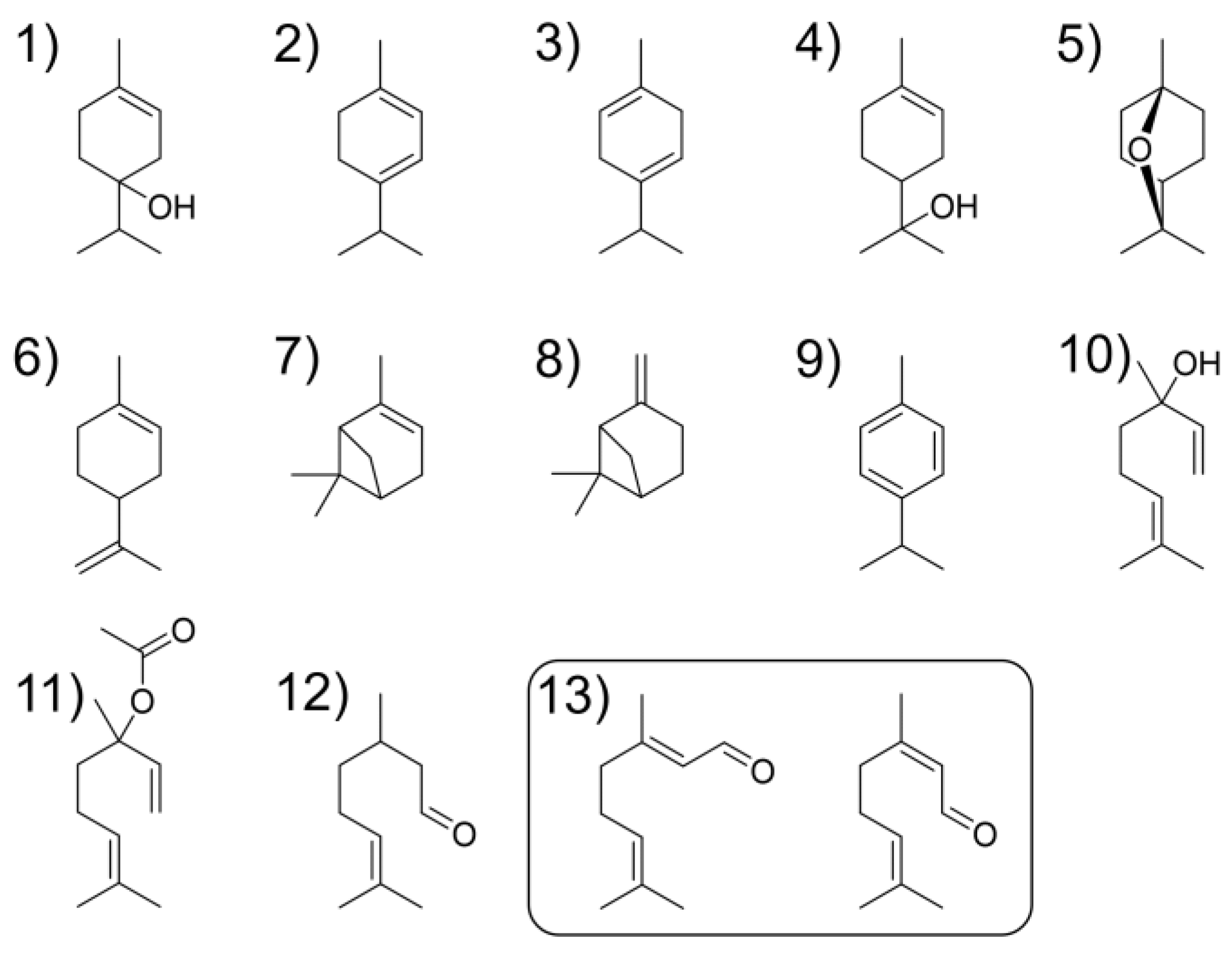
The molecular structures of the 14 effective components are shown in Figure 1. Neral and geranial are cis-trans isomers mixed in one reagent, citral. Therefore, 13 reagents were used as the target gases and are denoted as numbers 1–13 in Figure 1.

Figure 1.
Structural formulae of the effective components as target gases: (1) terpinen-4-ol, (2) α-terpinene, (3) γ-terpinene, (4) α-terpineol, (5) eucalyptol, (6) d-limonene, (7) α-pinene, (8) β-pinene, (9) p-cymene, (10) linalool, (11) linalyl acetate, (12) citronellal, and (13) citral (mixture of cis [neral]-trans [geranial] isomers).
All the target gases were generated from their solvents using a Gastec Permeator PD-1B gas generator (Ayase, Kanagawa, Japan), which can be exclusively used with diffusion vessels (D-tubes; D-02, D-03, D-04, and D-05), as shown in Figure S1 (Supplementary Materials). Table 3 lists the combinations of D-tubes (Levels 1–4) and their diffusion concentrations in the target gases. The concentration of the target gas depends on the type of D-tube, the temperature of the chamber in which the D-tube is placed, and the flow rate of the total flow. The temperature in PD-1b and the total flow rate were always 35 °C and 500 mL/min in this study. Therefore, the concentration of the target gas was controlled by the type of D-tube. The target gases were prepared in this manner because it was assumed that all the components would diffuse under the same gas generator in future applications. Single target gases and two types of mixed target gases (denoted as double gases) were analyzed. For a single gas, four concentrations of each reagent were prepared; therefore, 52 types of single gases (13 target gases × 4 concentrations) were used. For double gases, combinations of the two concentration levels (1 and 3) were prepared (13 target gases × 2 concentrations) and two reagents were selected (26C2). However, 13 pairs were excluded because they were a combination of levels 1 and 3 of the same gas; accordingly, 312 types of double gases (26C2–13) were used.
Table 3.
Concentrations of target gas prepared by the gas generator using four types of D-tubes.
2.3. Sensor Response Measurement
The sensor responses were measured using a flow apparatus and sensor system. Both sensor arrays C and L were equipped with sensor systems (Figure S2). The sensor systems controlled the applied voltage to the sensors (5 V: sensor array C) or working temperature (420 and 300 °C: sensor array L), and transferred sensor signals, i.e., resistances, to PCs via Bluetooth. The target gases were mixed with the carrier gas to maintain the specified concentrations. The total flow rate, N2/O2 ratio, humidity, and aspiration of gases from the sensor systems were maintained at 500 mL/min, 4, 60%, and 200 mL/min, respectively.
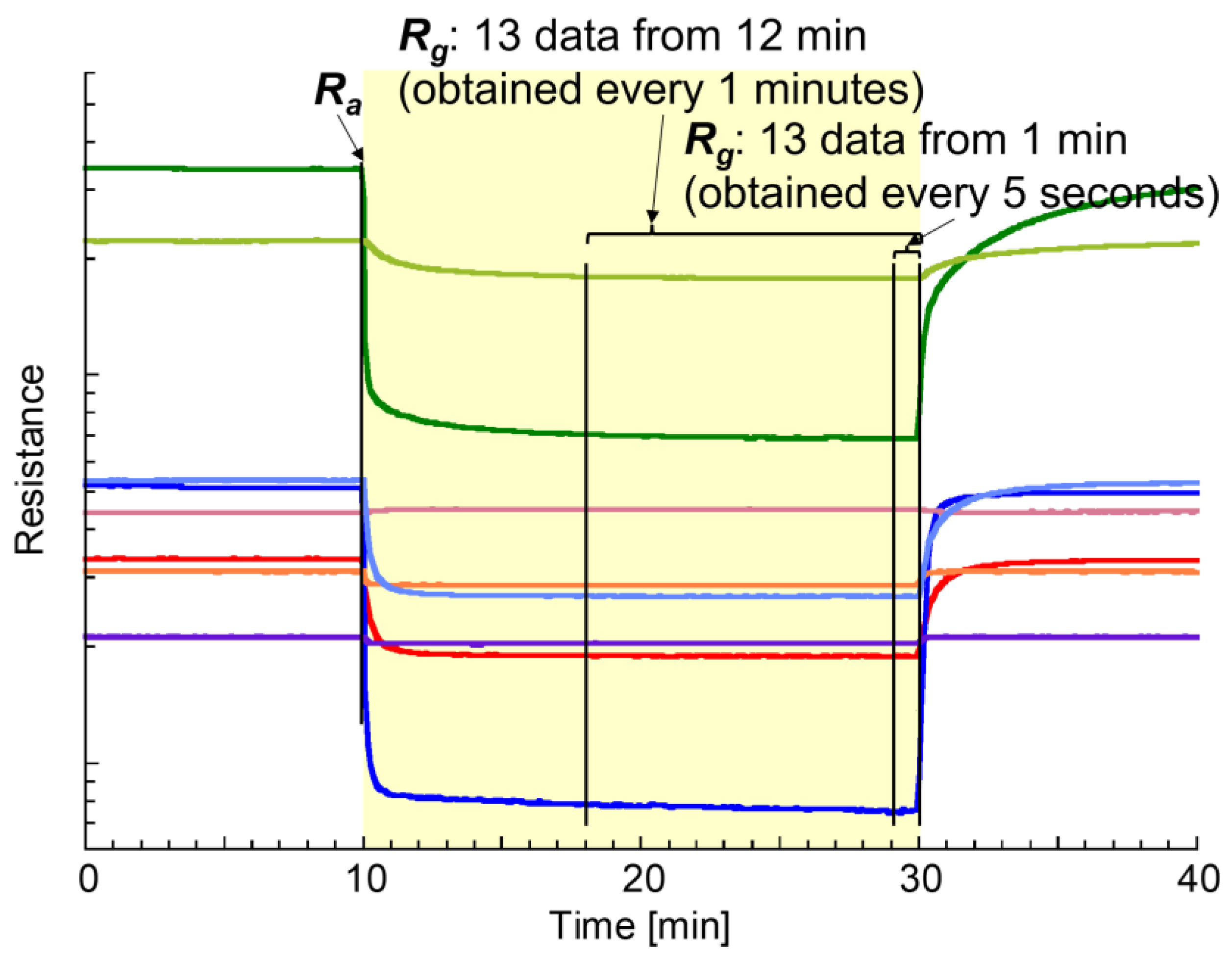
Figure 2 shows a model of the sensor responses to the target gas and the location of the data used for data analysis. The sensor response value, r, was collected 13 times after the introduction of each target gas for 20 min. The sensor response is defined in Equation (1):
where s and k are the sensor and data numbers, respectively. Moreover, rsk, Rask, and Rgsk are the sensor response, resistance immediately before introducing the target gas, and resistance upon introducing the target gas on sensor s and data number k, respectively.
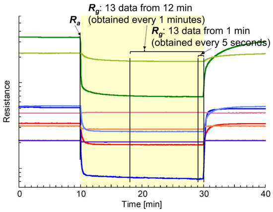
Figure 2.
Model showing the responses of eight sensors to the target gas and the location of the data used for data analysis. Yellowish region indicates target gas flowing into the sensor chamber.
As shown in the model in Figure 2, the resistances of the gas sensors significantly fluctuated just after the introduction of the target gas; however, slight fluctuations were also observed thereafter. In this study, two types of sensor response collection methods were employed: 13 Rg values were obtained every 1 min for 12 min, denoted as “12 min data”, or every 5 s for 1 min, denoted as “1 min data”, just before the end of the target gas introduction. The fluctuations in resistance during 1 min were extremely small compared to those during 12 min. A total of 676 data points (52 × 13 sensor responses r from Rg) from single gases and 4056 data points (312 × 13 sensor responses r from Rg) from double gases were collected for each type of sensor response collection method.
2.4. Data Analysis
2.4.1. Machine Learning
Machine learning was performed using Scikit-learn version 1.0.2 and TensorFlow version 2.4.0 in Python version 3.7.6. Sensor responses r in all data points were converted to their standardized values for machine learning,
where xsk is a standardization value of data number k on sensor number s, and and σs are the mean and standard deviation of r on sensor s, respectively.
A PCA was performed to investigate the characteristics of the datasets obtained from the two sensor arrays. The PCA was performed only on single gases because the inclusion of double gases resulted in too many classes and made classification difficult (with 676 data points). The PCA was performed according to Equations (S1)–(S6) in the Supplementary Materials.
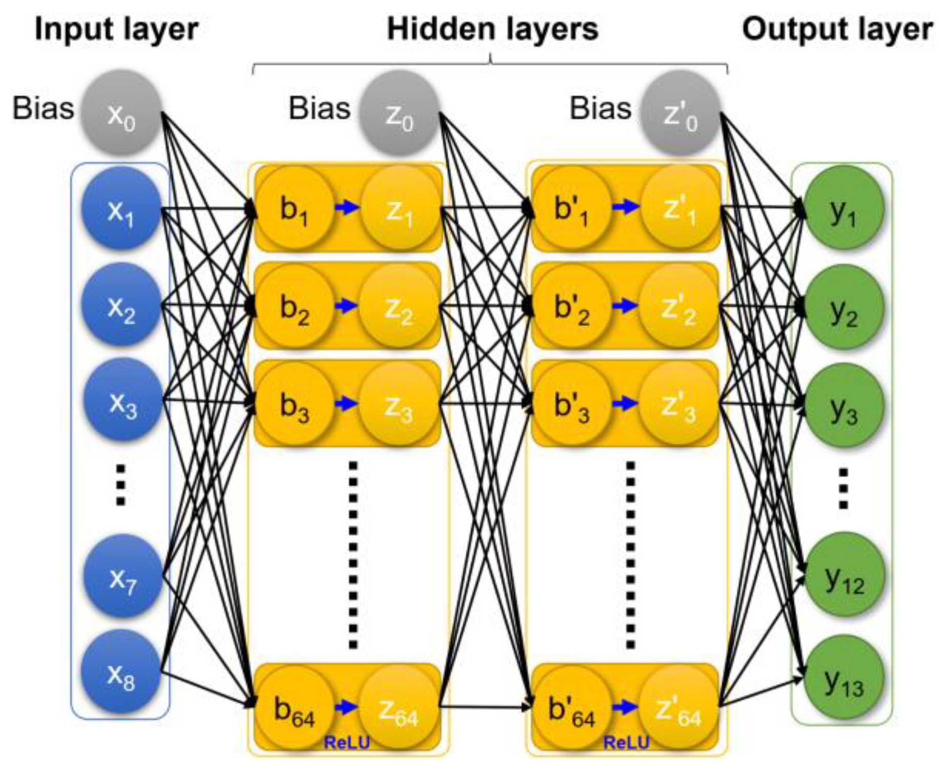
The ANN model is shown in Figure 3. The concentrations of target gases were predicted using the ANN. The structure of the neural network comprised an input layer with eight nodes (x1–x8) for the standardization values of sensor responses from eight sensors as explanatory variables; two hidden layers with 64 nodes (b1–b64 and b′1–b′64) with rectified linear units (ReLU; z1–z64 and z′1–z′64); and an output layer with 13 nodes (y1–y13) for the concentrations of the 13 target gases as objective variables. The ANN performed using 5-fold cross validation. All data points (676 + 4056 = 4732) were randomly divided into five parts, one of which was used as test data (946 or 947 data points) and the rest as training data (3786 or 3785 data points). First, all coefficients for moving data to the next layer in the ANN model (corresponding to the black arrows in Figure 3) were optimized using training data. Subsequently, all data points of the test data were substituted into the input layer for collecting the predicted concentrations of the 13 target gases from the output layer. By repeating the ANN five times with 5-fold cross-validation, each data point was the test data only once. Among the hyperparameters, the batch size was set to 32, and the number of epochs was the value at which the average loss function of the test data in the 5-fold cross-validation was minimized.

Figure 3.
Model of ANN used in the study.
2.4.2. Evaluating the Sensor Array Performance
Because the concentrations of the target gases in the test data were known, the prediction accuracy was evaluated by comparing the predicted concentrations with the correct concentrations. Based on the prediction accuracy, the performances of the two types of sensor arrays and two types of sensor response collection methods were evaluated. For single gases, the correct answer rates were determined based on whether the correct target gas was predicted at the highest concentration. Similarly, for double gases, the correct answer rates were determined based on whether the highest and second highest correct target gases were predicted at the highest and second highest concentrations, respectively. Moreover, the relationship between the correct and predicted concentrations for each target gas was shown, as well as the calculated slope (a) of approximate linear function, R-squared (R2) value, mean absolute error (MAE), and mean squared error (MSE).
3. Results and Discussion
3.1. Resistance Change as a Sensor Response
Figure 4 shows the dynamic resistance response of all sensors to single gases of citronellal (No. 12) and d-limonene (No. 6) and double gases of α-terpinene (No. 2) and d-limonene (No. 6), as examples. All the sensors in sensor array C were n-type semiconductor gas sensors that decreased in resistance in response to the target gases, whereas the two sensors in sensor array L were p-type semiconductor gas sensors that increased in resistance in response to the target gases. Figure 4a–d show the measurements acquired while decreasing the single gas concentration from levels 4 to 1. Because all responses were for the same target gas, the change in the resistance of each gas sensor decreased as the target gas concentration decreased.
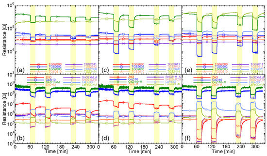
Figure 4.
Dynamic resistance responses: sensor array and target gas are (a) C and single gas No. 12, (b) L and single gas No. 12, (c) C and single gas No. 6, (d) L and single gas No. 6, (e) C and double gases Nos. 2 + 6, and (f) L and double gases Nos. 2 + 6, respectively. Concentration levels of the target gases are, in order, (a–d) Lvs. 4, 3, 2, and 1; (e,f) Lvs. 3 + 3, 3 + 1, 1 + 1, and 1 + 3.
In sensor array C, for TGS2602 and TGS2603, which have particularly large resistance changes as sensor responses, the value of resistance change decreased as the target gas concentration decreased. The other sensors in sensor array C exhibited minimal responses. The sensors included in sensor array C were manufactured for various purposes, as listed in Table 1. Sensors used to monitor fuel systems, such as liquified petroleum gas and methane, showed particularly low responses. Furthermore, TGS2602 and TGS2603 showed greater responses to number 6 than to number 12. The concentration ranges of the target gas numbers 1, 4, 10, 11, 12, and 13 were approximately one order of magnitude lower than those of the other target gases, as shown in Table 3. Because they are all polar molecules with alcohol, ester, or aldehyde functional groups, their volatility is reduced by intermolecular forces. Empirically, semiconductor sensors show a high response to gas species that have oxidizable functional groups, but this response is offset by the difference in concentration.
In sensor array L, because the two LaFeO3-based sensors were p-type semiconductors, the resistance changed as the sensor response increased when the target gas was introduced. Responses to number 12 from all sensors in sensor array L were better than those from TGS2602 and TS2603. These sensors were designed by considering conditions such as film thickness, which were optimized in past research. For the ZnO-based sensors, the response to number 12 was better than that of number 6. The other sensors appeared to have approximately the same response to numbers 6 and 12. Therefore, in sensor array L, the influence of the functional groups was greater than that of their concentration.
Figure 4e,f show the change in the resistance of each sensor against double gases, including numbers 2 and 6. The concentration combinations were levels 3 + 3, 3 + 1, 1 + 1, and 1 + 3, in the order shown in Figure 4e,f. Levels 3 + 1 and 1 + 3 had approximately the same level of resistance change, but the resistance change varied depending on the sensor. These results indicate that the relationship between the magnitude of the response of each sensor to the gas type and concentration was different.
3.2. Variation of Dataset in PCA
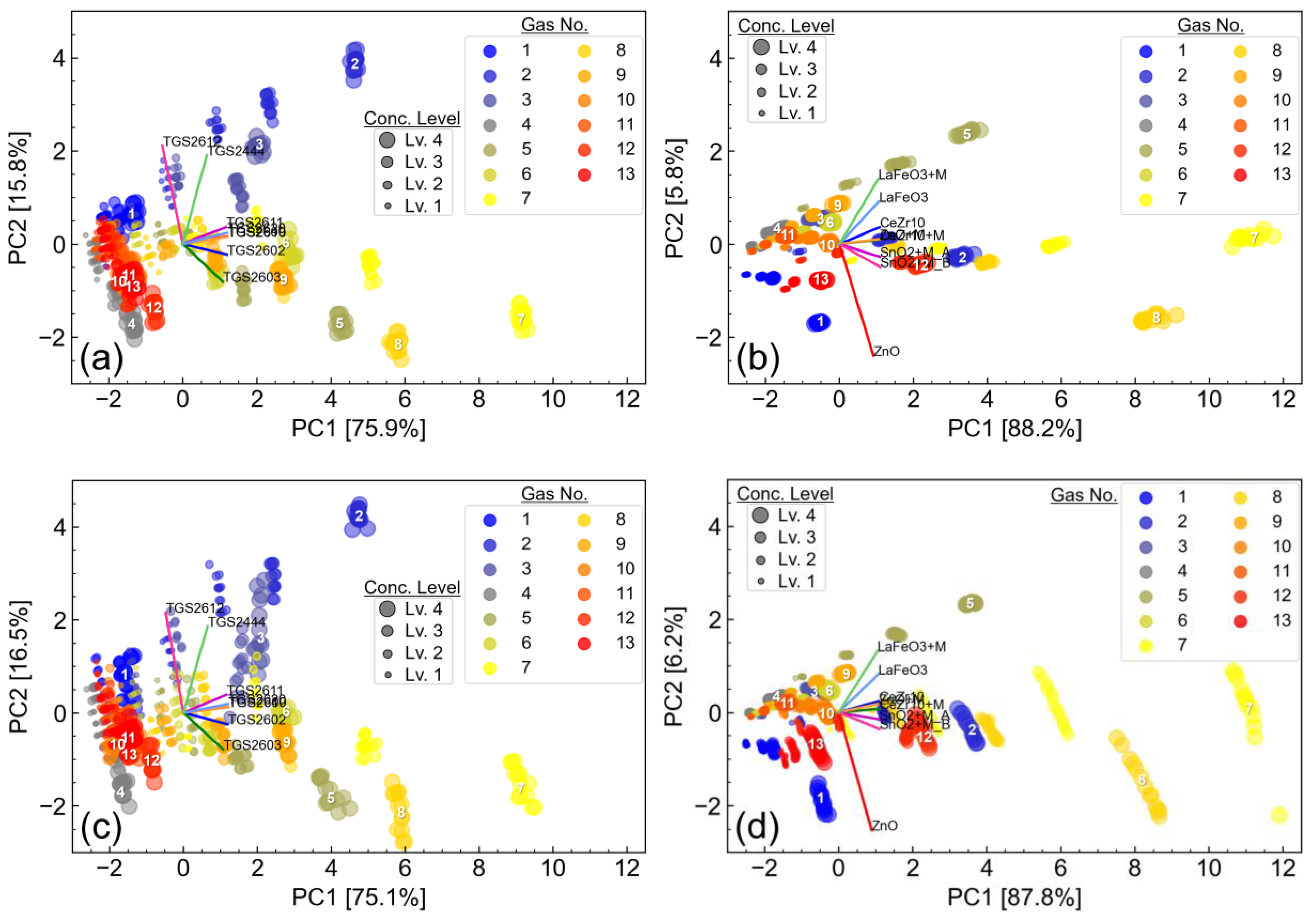
As described above, PCA is an effective method to easily check trends in a dataset as the scores can be graphically illustrated. Although a PCA cannot be performed to predict answers in classification and regression, the variance and reproducibility of the data can be easily checked from the graphs. Figure 5 shows the PCA scores and eigenvectors from the sensor responses for a single gas on sensor arrays C and L. The cumulative variance of the first and second principal components (PC1 and PC2) of all panels in Figure 5 was greater than 80%. The first two PCs are normally sufficient to retain the originality of the data [28]. Focusing on the eigenvectors, although the eigenvectors of TGS2600, TGS2610, and TGS2620, and CeZr10 + M and ZnO + M tend to overlap, the eigenvectors of the other sensors did not overlap in their respective directions. Therefore, each sensor generally had unique response characteristics for each target gas.
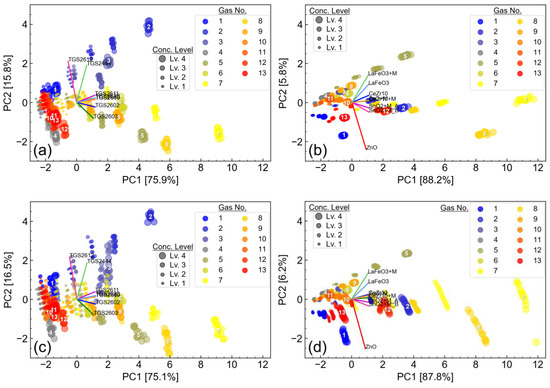
Figure 5.
PCA scores and eigenvectors: sensor array and dataset are (a) C and 1 min data, (b) L and 1 min data, (c) C and 12 min data, and (d) L and 12 min data, respectively. Numbers on plots from Lv. 4 indicate gas numbers.
The data in Figure 5a,b were from the 1 min data. The PCA scores for each target gas tended to converge in the direction of (0, –2) coordinates as the concentration decreased. Figure 5b, which shows the PCA score of sensor array L, indicates that the scores are generally independent at any concentration level for any target gas. However, in Figure 5a, which presents the PCA score of sensor array C, there are variations in the plot in the PC2 axis direction. For example, numbers 4, 10, 11, 12, and 13, which have alcohol, ester, and aldehyde functional groups, have overlapping plot areas and are difficult to discriminate. This is because the sensor responses of TGS2612 and TGS2444, whose eigenvectors strongly influenced the PC2 axis direction, were small and affected by variations in the noise level.
The data in Figure 5c,d were obtained from the 12 min data. In Figure 5c, which shows the PCA score of sensor array C, the scatter in the plots is even greater than that in Figure 5a, and the areas and overlap of the plots of the different gas species have expanded. Figure 5d, which shows the PCA score of sensor array L, displays that some plots varied in a direction parallel to the ZnO eigenvector. As shown in Figure 4b,d, particularly for ZnO, the resistance drifted during the introduction of the target gas. Thus, the influence of drift appeared when the interval was expanded to obtain the sensor response values.
3.3. Variation of Dataset in ANN
Unlike PCA, an ANN cannot visually confirm trends in the data contained in a dataset; however, it can obtain predictive results with high accuracy. The confusion matrices present the number of correct/wrong answers for each target gas type in the visualization, as shown in Figures S3–S6. In the confusion matrices, the results are organized into the number of correct answers from the single gas, the highest concentration of the double gas, and the second highest concentration of the double gas. Table 4 lists the correct answer rates for the 14 effective components in the ANN. A correct answer rate of over 90% was obtained under all conditions, but the correct answer rate was higher for sensor array L than for sensor array C. However, even for sensor array C, the plot areas overlapped in the PCA (Figure 5), but all single gases were correct in the ANN. Therefore, an ANN is an excellent analysis method for discriminating odors in gas sensors. The correct answer rates for double gases were lower than those for single gases in all datasets. Furthermore, the correct answer rate for the second concentration component was lower than the first concentration component. The presence of coexisting components and an increase in the concentration of them could have a greater influence on the correct answer rate.
Table 4.
Correct answer rate of effective components in ANN.
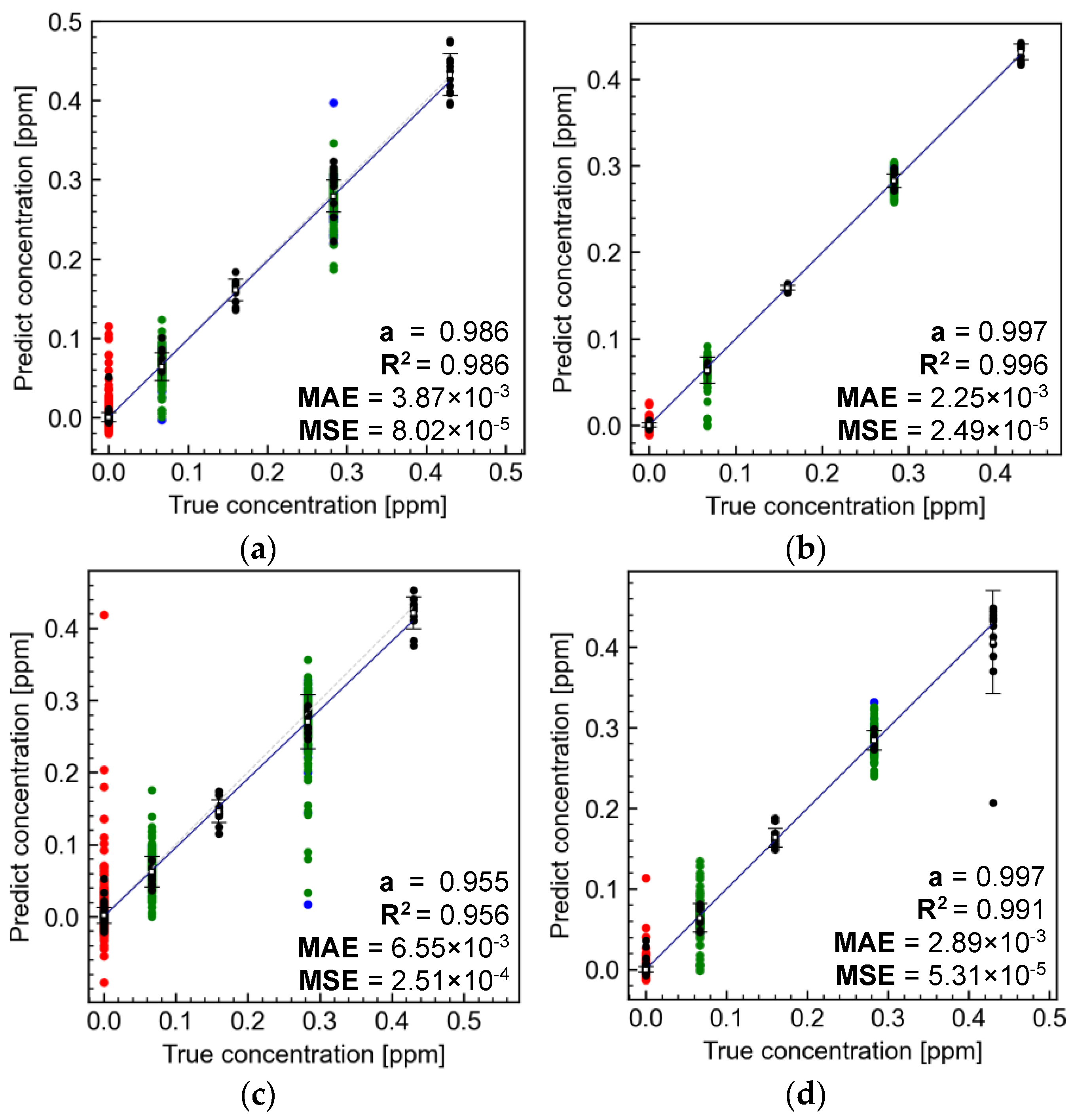
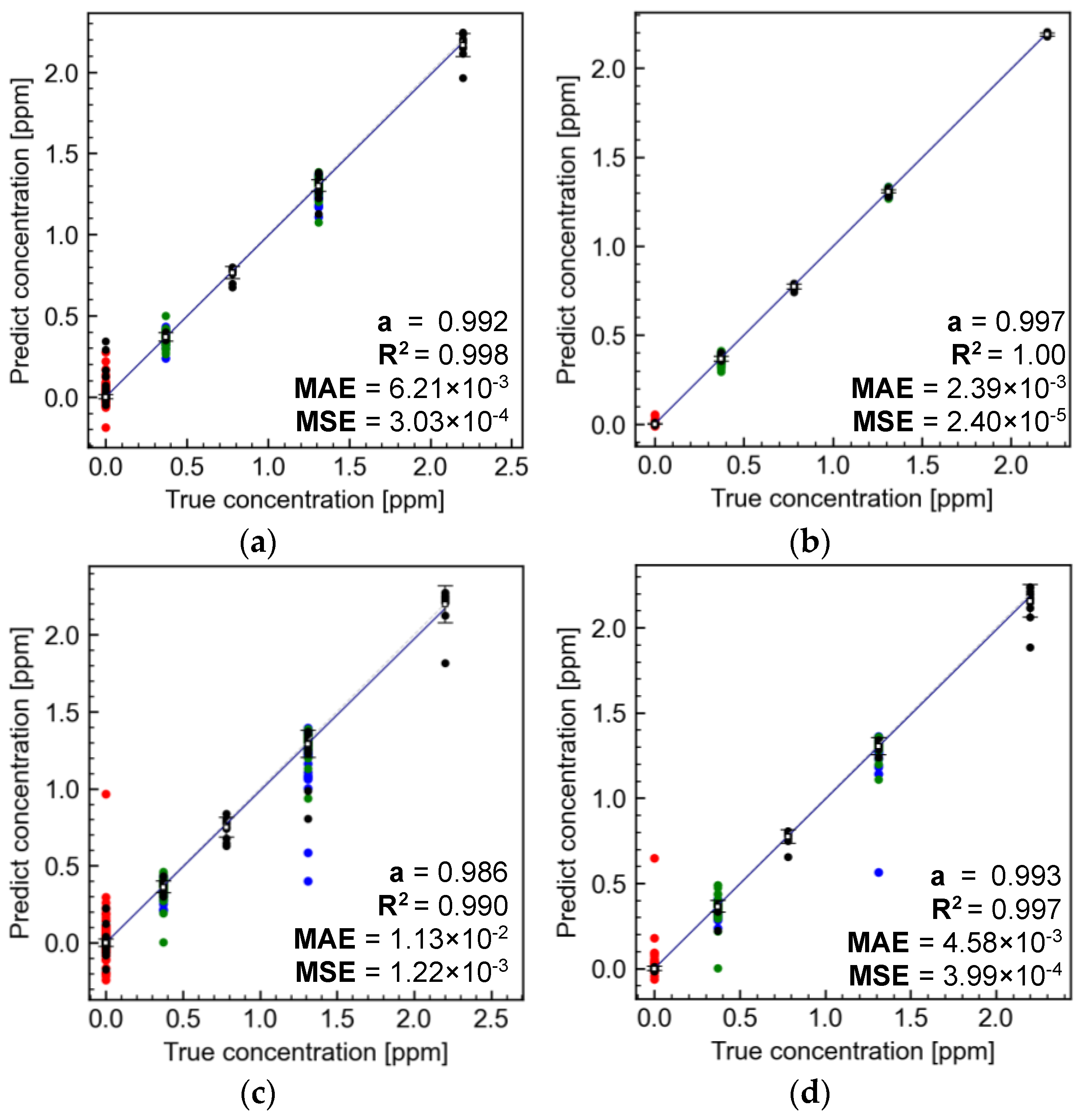
Figure 6 and Figure 7 show the relationship between the true and predicted concentrations for numbers 12 and 6, respectively. The results for all the target gases are shown in Figures S7–S10. The difference between Figure 6a,c or Figure 6b,d is the interval used to obtain the sensor response values for the datasets. In both cases, the 1 min dataset, which has a narrower data range and less drift influence, had smaller plot variations, and the values listed in the panels were also better. The difference between Figure 6a,b or Figure 6c,d is the sensor array. In both cases, sensor array L had smaller plot variations, and the values listed in the panel were also better. Furthermore, in both panels, the variation in the predicted concentration plots for a single gas (black) was lower than that for double gases (blue, green, and red). These results show the same tendencies as the correct answer rates shown in Table 4. Figure 7 shows number 6, which had a larger concentration range than number 12 in Figure 6. As shown in Figure 6, the differences in the range of the data acquired by the dataset and in the sensor arrays showed the same trend. In addition, the results in Figure 7 are better than those in Figure 6, indicating that higher gas concentrations afforded more accurate results.
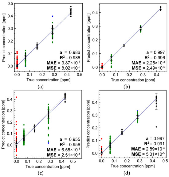
Figure 6.
Relationship diagram between true and predicted concentrations for target gas No. 12 using (a,b) 1 min data and (c,d) 12 min data on sensor arrays (a,c) C and (b,d) L. Plot colors are black: single gas, blue: highest concentration component of double gases, green: second highest concentration component of double gas, and red: other double gases.
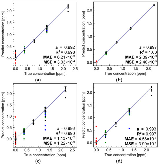
Figure 7.
Relationship diagram between true and predicted concentrations for target gas No. 6 using (a,b) 1 min data and (c,d) 12 min data on sensor arrays (a,c) C and (b,d) L. Plot colors are black: single gas, blue: highest concentration component of double gases, green: second highest concentration component of double gas, and red: other double gases.
3.4. Importance of Gas Sensor Selection
Sensor array L exhibited better results than sensor array C as the benchmark array. All 14 components of the target gas were terpenes or similar. The responses of semiconductor sensors can be categorized into gas groups [35]. Therefore, the discrimination of terpene gases was expected to be more difficult than that of gases from other groups. Sensor array C included all general n-type semiconductor sensors, whereas sensor array L included not only general semiconductor sensors, such as n-type [33,36] and p-type [37,38,39], but also cerium oxide bulk-response sensors [34]. The resistance change mechanism in a traditional n-type semiconductor sensor involves a change in the electron density at the grain boundaries of n-type semiconductor particles by the oxidation of the target gases on the surface of the grains. In contrast, the resistance change mechanism in a p-type semiconductor sensor involves a change in the hole density at the grain boundaries of n-type semiconductor particles. The resistance change mechanism in the bulk-responsive sensor is that the odor molecules consume the lattice oxygen in the cerium oxide particles to undergo oxidation and generate oxygen vacancies, which diffuse throughout the bulk without accumulating on the particle surface [34]. In addition, sensor array L was not superior in terms of resistance change to number 6 (Figure 4d) compared to number 12 (Figure 4b). However, the relationship between the actual and predicted concentrations in the ANN between numbers 12 (Figure 6b,d) and 6 (Figure 7b,d) were both excellent. Based on these results, the combination of sensors with different response principles results in improved accuracy for the discrimination of effective components. To obtain high accuracy, it is important to determine the differences in the sensor response for each gas condition (not necessarily the magnitude of the sensor response).
Even with such an excellent sensor array, the results showed large variations when the data acquisition time intervals were different. For future applications, it is desirable to maintain a constant measurement time within the range permitted by operational conditions.
4. Conclusions
We discriminated between and measured the concentrations of 14 effective components of aroma essential oils from single and double gases using sensor arrays C and L. Datasets were obtained from sensor signals in response to each target gas. We also considered the time interval for data acquisition. The sensors in sensor array L generally exhibited stronger responses than those in sensor array C. The PCA revealed that the plots from sensor array C had variations and their regions overlapped; however, in sensor array L, the plots were independent at any concentration level for all the target gases. In a detailed analysis using a neural network, the correct answer rate was over 90% for all dataset conditions. Under all conditions, the correct answer rate and accuracy of predicting the concentration of components were higher for sensor array L than for sensor array C. This result occurred because sensor array L combined several sensors that possessed different semiconductor sensor principles and high sensing properties for the components. However, it is desirable to ensure that the time intervals for acquiring the dataset are as consistent as possible.
Supplementary Materials
The following supporting information can be downloaded at: https://www.mdpi.com/article/10.3390/app14198859/s1, including Figures S1–S10 and Table S1.
Author Contributions
Conceptualization, T.I., W.S., J.A. and N.T.; methodology, T.I.; software, T.I.; formal analysis, T.I.; investigation, T.I.; data curation, T.I.; writing—original draft preparation, T.I.; writing—review and editing, P.G.C., Y.M., J.A. and N.T.; supervision, W.S.; project administration, N.T.; funding acquisition, N.T. All authors have read and agreed to the published version of the manuscript.
Funding
This research received no external funding.
Institutional Review Board Statement
Not applicable.
Informed Consent Statement
Not applicable.
Data Availability Statement
The original contributions presented in the study are included in the article and Supplementary Materials, further inquiries can be directed to the corresponding author.
Acknowledgments
The authors thank Ryoko Sako (AIST) for her technical support in the preparation of gas sensor elements and the analysis of sensing properties.
Conflicts of Interest
Authors Junichirou Arai and Nobuaki Takeda were employed by the company Daikin Industries, Ltd. The remaining authors declare that the research was conducted in the absence of any commercial or financial relationships that could be construed as a potential conflict of interest.
References
- Sasannejad, P.; Saeedi, M.; Shoeibi, A.; Gorji, A.; Abbasi, M.; Foroughipour, M. Lavender essential oil in the treatment of migraine headache: A placebo-controlled clinical trial. Eur. Neurol. 2012, 67, 288–291. [Google Scholar] [CrossRef] [PubMed]
- Yogi, W.; Tsukada, M.; Sato, Y.; Izuno, T.; Inoue, T.; Tsunokawa, Y.; Okumo, T.; Hisamitsu, T.; Sunagawa, M. Influences of Lavender Essential Oil Inhalation on Stress Responses during Short-Duration Sleep Cycles: A Pilot Study. Healthcare 2021, 9, 909. [Google Scholar] [CrossRef] [PubMed]
- Karadag, E.; Samancioglu, W.; Ozden, E.; Bakir, E. Effects of aromatherapy on sleep quality and anxiety of patients. Nurs. Crit. Care 2015, 22, 105–112. [Google Scholar] [CrossRef] [PubMed]
- Firoozeei, T.S.; Feizi, A.; Rezaeizadeh, H.; Zargaran, A.; Roohafza, H.R.; Karimi, M. The antidepressant effects of lavender (Lavandula angustifolia Mill.): A systematic review and meta-analysis of randomized controlled clinical trials. Complement. Ther. Med. 2021, 59, 102679. [Google Scholar] [CrossRef] [PubMed]
- Ballard, C.G.; O’Brien, J.T.; Reichelt, K.; Perry, E.K. Aromatherapy as a Safe and Effective Treatment for the Management of Agitation in Severe Dementia: The Results of a Double-Blind, Placebo-Controlled Trial with Melissa. J. Clin. Psychiatry 2002, 63, 553–558. [Google Scholar] [CrossRef] [PubMed]
- Kennedy, D.O.; Wake, G.; Savelev, S.; Tildesley, N.T.J.; Perry, E.K.; Wesnes, K.A.; Scholey, A.B. Modulation of mood and cognitive performance following acute administration of single doses of Melissa officinalis (Lemon balm) with human CNS nicotinic and muscarinic receptor-binding properties. Neuropsychopharmacology 2003, 28, 1871–1881. [Google Scholar] [CrossRef] [PubMed]
- Akhondzadeh, S.; Noroozian, M.; Mohammadi, M.; Ohadinia, S.; Jamshidi, A.H.; Khani, M. Melissa officinalis extract in the treatment ofpatients with mild to moderate Alzheimer’s disease:a double blind, randomised, placebo controlled trial. J. Neurol Neurosurg. Psychiatry 2003, 74, 863–866. [Google Scholar] [CrossRef]
- Kennedy, D.O.; Little, W.; Scholey, A.B. Attenuation of laboratory-induced stress in humans after acute administration of Melissa officinalis (lemon balm). Psychosom. Med. 2004, 66, 607–613. [Google Scholar] [CrossRef]
- Tanaka, Y.; Kikuzaki, H.; Nakatani, N. Antibacterial activity of essential oils and oleoresins of spices and herbs against pathogens bacteria in upper airway respiratory tract. Jpn. J. Food Chem. 2002, 9, 67–76. [Google Scholar]
- Hart, P.H.; Brand, C.; Carson, F.; Riley, T.V.; Prager, R.H.; Finlay-Jones, J.J. Terpinen-4-ol, the main component of the essential oil of Melaleuca alternifolia (tea tree oil), suppresses inflammatory mediator production by activated human monocytes. Inflamm. Res. 2000, 49, 619–626. [Google Scholar] [CrossRef] [PubMed]
- Lee, C.-J.; Chen, L.-W.; Chen, L.-G.; Chang, T.-L.; Huang, C.-W.; Huang, M.-C.; Wang, C.-C. Correlations of the components of tea tree oil with its antibacterial effects and skin irritation. J. Food Drug Anal. 2013, 21, 169–176. [Google Scholar] [CrossRef]
- Juergens, U.R.; Dethlefsen, U.; Steinkamp, G.; Gillissen, A.; Repges, R.; Vetter, H. Anti-inflammatory activity of 1.8-cineol (eucalyptol) in bronchial asthma: A double-blind placebo-controlled trial. Respir. Med. 2003, 97, 250–256. [Google Scholar] [CrossRef] [PubMed]
- Reis, R.; Orak, D.; Yilmaz, D.; Cimen, H.; Sipahi, H. Modulation of cigarette smoke extract-induced human bronchial epithelial damage by eucalyptol and curcumin. Human Experiment. Toxicol. 2021, 40, 1445–1462. [Google Scholar] [CrossRef]
- Essential Oils Market Size, Share & Trends Analysis Report By Product (Orange, Cornmint, Eucalyptus), by Application (Medical, Food & Beverages, Spa & Relaxation), by Sales Channel, by Region, and Segment Forecasts, 2024–2030. Available online: https://www.grandviewresearch.com/industry-analysis/essential-oils-market#:~:text=The%20global%20essential%20oils%20market,CAGR)%20of%207.6%25%20from%202024 (accessed on 2 September 2024).
- Koike, K. Phytotherapy; Kyoto Hirokawa, Co.: Kyoto, Japan, 2016; ISBN 978-4-906992-75-1. (In Japanese) [Google Scholar]
- Lavender Oil. Available online: https://aromesparfums.com/products/lavender-true (accessed on 14 December 2023).
- Pokajewicz, K.; Biało’n, M.; Svydenko, L.; Fedin, R.; Hudz, N. Chemical Composition of the Essential Oil of the New Cultivars of Lavandula angustifolia Mill. Bred in Ukraine. Molecules 2021, 26, 5681. [Google Scholar] [CrossRef] [PubMed]
- Melissa Oil. Available online: https://aromesparfums.com/products/melissa (accessed on 14 December 2023).
- Nurzyńska-Wierdak, R.; Bogucka-Kocka, A.; Szymczak, G. Volatile constituents of Melissa officinalis leaves determined by plantage. Nat. Prod. Commun. 2014, 9, 703–706. [Google Scholar]
- Tea Tree Oil. Available online: https://www.teatreeoil.co.jp/certificate-of-analysis-mc7e18/ (accessed on 14 December 2023).
- Carson, C.F.; Hammer, K.A.; Riley, T.V. Melaleuca alternifolia (Tea Tree) oil: A review of antimicrobial and other medicinal properties. Clin. Microbiol. Rev. 2006, 19, 50–62. [Google Scholar] [CrossRef]
- Eucalyptus. Available online: https://www.florihana.co.jp/?pid=159536207 (accessed on 14 December 2023).
- Sebei, K.; Sakouhi, F.; Herchi, W.; Khouja, M.L.; Boukhchina, S. Chemical composition and antibacterial activities of seven Eucalyptus species essential oils leaves. Biol. Res. 2015, 48, 7. [Google Scholar] [CrossRef] [PubMed]
- Kim, H.-J.; Lee, J.-H. Highly sensitive and selective gas sensors using p-type oxide semiconductors: Overview. Sens. Actuators B Chem. 2014, 192, 607–627. [Google Scholar] [CrossRef]
- Dey, A. Semiconductor metal oxide gas sensors: A review. Sens. Actuators B Chem. 2018, 229, 206–217. [Google Scholar] [CrossRef]
- Rasekh, M.; Karami, H.; Wilson, A.D.; Gancarz, M. Classification and Identification of Essential Oils from Herbs and Fruits Based on a MOS Electronic-Nose Technology. Chemosensors 2021, 9, 142. [Google Scholar] [CrossRef]
- Gaggiotti, S.; Palmieri, S.; Pelle, F.D.; Sergi, M.; Cichelli, A.; Mascini, M.; Compagnone, D. Piezoelectric peptide-hpDNA based electronic nose for the detection of terpenes; Evaluation of the aroma profile in different Cannabis sativa L. (hemp) samples. Sens. Actuators B Chem. 2020, 308, 127697. [Google Scholar] [CrossRef]
- Srivastava, A.; Dravid, V.P. On the performance evaluation of hybrid and mono-class sensor arrays in selective detection of VOCs: A comparative study. Sens. Actuators B Chem. 2006, 117, 244–252. [Google Scholar] [CrossRef]
- Jeon, J.-Y.; Choi, J.-S.; Yu, J.-B.; Lee, H.-R.; Jang, B.-K.; Byun, J.-G. Sensor array optimization techniques for exhaled breath analysis to discriminate diabetics using an electronic nose. ETRI J. 2018, 40, 802–812. [Google Scholar] [CrossRef]
- Vajdi, M.; Varidi, M.J.; Varidi, M.; Mohebbi, M. Using electronic nose to recognize fish spoilage with an optimum Classifier. J. Food. Meas. Charact. 2019, 13, 1205–1217. [Google Scholar] [CrossRef]
- Shiba, K.; Imamura, G.; Yoshikawa, G. Odor-Based Nanomechanical Discrimination of Fuel Oils Using a Single Type of Designed Nanoparticles with Nonlinear Viscoelasticity. ACS Omega 2021, 6, 23389–23398. [Google Scholar] [CrossRef] [PubMed]
- Zhang, J.; Xue, Y.; Sun, Q.; Zhang, T.; Chen, Y.; Yu, W.; Xiong, Y.; Wei, X.; Yu, G.; Wan, H.; et al. A miniaturized electronic nose with artificial neural network for anti-interference detection of mixed indoor hazardous gases. Sens. Actuators B Chem. 2021, 326, 128822. [Google Scholar] [CrossRef]
- Itoh, T.; Nakashima, T.; Akamatsu, T.; Izu, N.; Shin, W. Nonanal gas sensing properties of platinum, palladium, and gold-loaded tin oxide VOCs sensors. Sens. Actuators B Chem. 2013, 187, 135–141. [Google Scholar] [CrossRef]
- Itoh, T.; Izu, N.; Akamatsu, T.; Shin, W.; Miki, Y.; Hirose, Y. Elimination of Flammable Gas Effects in Cerium Oxide Semiconductor-Type Resistive Oxygen Sensors for Monitoring Low Oxygen Concentrations. Sensors 2015, 15, 9427–9437. [Google Scholar] [CrossRef]
- Kadosaki, M.; Sakai, Y.; Tamura, I.; Matsubara, I.; Itoh, T. Development of Oxide Semiconductor Thick Film Gas Sensor for the Detection of Total Volatile Organic Compounds. Electron. Commun. Jpn. 2008, 128, 125–130. [Google Scholar] [CrossRef]
- Krishna, K.G.; Umadevi, G.; Parne, S.; Pothukanuri, N. Zinc oxide based gas sensors and their derivatives: A critical review. J. Mater. Chem. 2023, 11, 3906–3925. [Google Scholar] [CrossRef]
- Dai, Z.; Lee, C.-S.; Kim, B.-Y.; Kwak, C.-H.; Yoon, J.-W.; Jeong, H.-M.; Lee, J.-H. Honeycomb-like Periodic Porous LaFeO3 Thin Film Chemiresistors with Enhanced Gas-Sensing Performances. ACS Appl. Mater. Interfaces 2014, 6, 16217–16226. [Google Scholar] [CrossRef] [PubMed]
- Jaouali, I.; Hamrouni, H.; Moussa, N.; Nsib, M.F.; Centeno, M.A.; Bonavita, A.; Neri, G.; Leonardi, S.G. LaFeO3 ceramics as selective oxygen sensors at mild temperature. Ceram. Int. 2018, 44, 4183–4189. [Google Scholar] [CrossRef]
- Thirumalairajan, S.; Girija, K.; Mastelaro, V.R.; Ponpandian, N. Surface Morphology-Dependent Room-Temperature LaFeO3 Nanostructure Thin Films as Selective NO2 Gas Sensor Prepared by Radio Frequency Magnetron Sputtering. ACS Appl. Mater. Interfaces 2014, 6, 13917–13927. [Google Scholar] [CrossRef]

Disclaimer/Publisher’s Note: The statements, opinions and data contained in all publications are solely those of the individual author(s) and contributor(s) and not of MDPI and/or the editor(s). MDPI and/or the editor(s) disclaim responsibility for any injury to people or property resulting from any ideas, methods, instructions or products referred to in the content. |
© 2024 by the authors. Licensee MDPI, Basel, Switzerland. This article is an open access article distributed under the terms and conditions of the Creative Commons Attribution (CC BY) license (https://creativecommons.org/licenses/by/4.0/).