Improving Raman-Based Models for Real-Time Monitoring the CHO Cell Culture Process with Effective Variable Selection Strategies

Abstract

Research has shown that Raman spectroscopy could be applied to monitor various components in mammalian cell culture in real time. In the process of application, it is necessary to ensure the performance of the Raman-based model. The variable selection strategy is an effective method that significantly influences the model performance and simplification. In this study, different variable selection strategies were evaluated, and the optimal variable selection strategy was determined for monitoring the CHO cell culture process. Firstly, a wide variety of spectral regions involving the Raman fingerprinting region and the C-H stretching region were investigated. Secondly, six different variable selection algorithms were meticulously assessed. Thirdly, the combination of different variable selection algorithms was used to improve model performance and simplify the model. Finally, the monitoring of cell culture processes was implemented. The findings underscored that commonly used spectral regions could improve the model performance but could not simplify the model well. Moving-window partial least square (MWPLS), genetic algorithm (GA), and random frog (RF) are more suitable for Raman modeling of the cell culture process, but they must be used after the spectral region selection. The combination of three variable selection algorithms (MWPLS-GA-RF) improved the model’s performance by 16–70% by selecting 30–60 variables, effectively simplifying the model. For glucose, lactate, viable cell density, and ammonium ion, real-time monitoring was performed well. This study will be helpful for researchers to select suitable variable selection strategies for building models for the real-time monitoring of cell culture.

1. Introduction

Therapeutic proteins, such as monoclonal antibodies, play an increasingly important role in the field of life sciences and health. Mammalian cells, particularly Chinese hamster ovary (CHO) cells, are the main force in the production of therapeutic proteins. Mammalian cell lines are capable of adding complexity to biologics through the post-translational modification of proteins [1]. However, these products are produced in relatively small quantities due to the highly specialized culture conditions and their susceptibility to reduced productivity or cell death from even slight deviations in these conditions [2]. The cell culture process seriously affects the yield and quality of therapeutic proteins. Conventionally, sampling the culture solution in the bioreactor for measuring metabolite concentrations and cell density introduces risks of contamination and analytical delays. For commercial production, real-time monitoring of primary metabolites and biomass is pivotal to ensure successful cell culture [3]. To circumvent the need for bioreactor sampling and attain real-time component information, Raman spectroscopy, as a potent process analytical technology (PAT) tool, has been extensively explored in upstream bioprocess manufacturing [4]. Its applicability stems from the weak scattering of water, which allows it to operate in aqueous culture media. Leveraging the multivariate data analysis, a multitude of studies have demonstrated Raman spectroscopy’s capability to monitor key components in the CHO cell culture. For instance, Webster et al. [5] developed generic Raman models for glucose (Gluc), lactate (Lac), ammonium ion (NH₄⁺), viable cell density (VCD), and total cell density for a GS-KO^TM CHO Platform Process using partial least squares (PLS) regression. Tulsyan et al. [6] proposed a novel machine-learning procedure based on just-in-time learning (JITL) to calibrate generic Raman models for the real-time monitoring of critical cell culture performance parameters. Additionally, some studies have focused on enhancing cell growth by integrating Raman spectroscopy with controllers to manage cell culture processes. For example, Raman spectroscopy has been employed to control glucose concentration [7], tune monoclonal antibody galactosylation [8], or maintain viable cell density at target levels [9].

Complications arise from the complex sample matrix and interactions between multiple components, leading to significant spectral shifts and weaker characteristic peak of the molecules of interest [10]. Some spectral regions are redundant, noisy, or irrelevant, undermining the reliability of key component predictions [11,12,13]. Limited implementation of Raman spectroscopy has been observed in commercial production [14], so it is necessary to study how to improve the prediction accuracy of Raman-based models. In addition, the number of Raman data collected during cell culture is substantial. Each Raman spectrum contains thousands of data points, and each batch of cell cultures produces thousands of spectra, posing a challenge for computer performance. Therefore, reducing spectral variables and simplifying Raman-based models are more conducive to the application of Raman spectroscopy in the monitoring and controlling of cell culture processes. Variable selection could reduce spectral variables used for modeling and improve model performance through excluding interfering bands and irrelevant regions. The effectiveness of enhancing model performance by variable selection has been proven [15].

During the development of Raman-based models, certain spectral regions have been employed, encompassing the Raman fingerprint and C-H stretching regions. These Raman spectral regions involve structured chemical variations and biochemical information, corresponding to the fingerprint region of organic compounds and the C-H contributions. However, there is no universal approach for the selection of these spectral regions. Different researchers have selected different spectral ranges, adhering to certain guiding principles, such as experiential insights [6], capturing the organic compounds’ fingerprint region [9], circumventing the lambda region [16], omitting regions with low signal-to-noise ratios [17], or excluding the Rayleigh scattering of the excitation source [18].

Table 1. The spectral regions used for Raman-based models in cell culture from the literature.

Spectral Range	N	Analyzed Components	Literature
800–1800 cm−1	1001	key biochemical values, VCD	[9]
500–1700 cm−1	1201	Gluc, Lac	[19]
400–1600 cm−1	1201	Gluc, Lac	[8]
400–1800 cm−1	1401	Gluc, Lac, titer	[20]
440–1860 cm−1	1421	VCD, Lac, NH4+, amino acids	[17]
350–1775 cm−1	1426	Gluc, Lac, VCD	[21]
321–1890 cm−1	1570	Gluc, Lac, amino acids	[22]
350–1775 cm−1, 2800–3000 cm−1	1627	Gluc, Lac	[23]
415–1800 cm−1, 2800–3100 cm−1	1687	VCD, viability, cell diameter	[24]
300–1850 cm−1, 2900–3200 cm−1	1852	Gluc, Lac, Glu, VCD	[25]
415–1850 cm−1, 1860–2100 cm−1, 2800–3100 cm−1	1978	Gluc, Lac, NH4+	[16]
500–3100 cm−1	2601	Gluc, phenylalanine	[7]
400–3200 cm−1	2801	Gluc, VCD, Lac, NH4+	[26]

N represents the number of selected variables.

presents different spectral ranges used for modeling in cell culture, and the numbers of selected spectral variables vary from 1001 to 2801. These studies all employed a Kaiser Raman spectrometer to collect spectra with the same resolution and similar raw spectral range, but different spectral regions were selected to represent the Raman fingerprint regions and C-H stretching regions, potentially leading to confusion among researchers. These spectral regions were used to build models for various components, such as Gluc, Lac, VCD, NH₄⁺, and protein titer, but explanations were not provided as to why the specific region was chosen for a certain component. Considering the specificity of Raman-based models, different spectral regions should be assigned to different analyzed components.

Considering that it is difficult to manually assign specific spectral variables to each analyzed component in a complex system, variable selection algorithms can be useful for choosing spectral variables that are sensitive to chemical changes in the matrix [21]. According to the literature [27], variable selection algorithms can be categorized into three main groups: filter methods, wrapper methods, and embedded methods. Filter methods involve variable selection based on a defined threshold; examples include Pearson’s correlation coefficient method (PCC) and variable importance in projection (VIP). Wrapper methods employ an iterative process to filter variables and include techniques like uninformative variable elimination method (UVE) [28], moving-window partial least square (MWPLS), and genetic algorithm (GA). Within the wrapper methods’ category, UVE and MWPLS are classified as dynamic wrapper methods, while GA is considered a randomized wrapper method. Lastly, embedded methods are integrated into modified algorithms, such as random forest (RF). Santos et al. [29] improved the predictive performance of PLS models through variable selection algorithms, including VIP and forward-interval partial least squares (iPLS), compared to models based on whole spectra or those driven by chemical information alone. In addition, combining different variable selection algorithms takes advantage of the complementarity between them. Firstly, spectral variables are selected coarsely, and then these selected spectral variables are chosen finely. Such a variable selection strategy is usually better than using a single variable selection algorithm. Wang et al. [30] used the UVE-CARS combination method to select spectral variables, which effectively predicted and visualized the concentration of total flavonoids in fruits. Yu et al. [31] studied four combination methods, IPLS-VIP-GA, IPLS-VIP-IRIV, IPLS-MVCPA-GA, and IPLS-MVCPA-IRIV, and the results showed that these methods had a better performance than a single variable selection algorithm. Different variable selection algorithms and their combinations have been used in various studies, with varying results [15,32,33]. Using only Raman characteristic peaks or a single variable selection algorithm to construct the monitoring model may yield one-sided results [13]. It is meaningful to investigate different variable selection algorithms and their combinations to effectively improve the Raman model performance during cell culture.

In this study, we provided a comprehensive assessment of various variable selection strategies, including selection from different spectral regions, the use of different variable selection algorithms, and combination methods. It is important to determine which variable selection strategy is optimal and how many variables should be chosen to simplify the model and enhance its performance. An inappropriate variable selection strategy may not improve model performance and can lead to an unrobust model. Selecting too many spectral variables may leave interference and irrelevant regions in the model, reducing the effectiveness of simplification. Conversely, selecting too few spectral variables might remove those related to structural changes in the analyzed component, leading to inaccurate or unrobust models. Therefore, studying the impact of different variable selection strategies and the number of selected spectral variables on Raman-based model performance is meaningful. In this study, we aim to identify the most suitable variable selection strategy for Raman-based models in CHO cell culture processes, which can simplify the models, enhance their predictive capabilities, and promote a deeper understanding of the data.

2. Materials and Methods

2.1. Cell Culture

A CHO-S cell line from the working cell bank established by Hisun Biopharmaceutical Co. Ltd. was used to produce a biosimilar of adalimumab during commercial-scale manufacturing [34,35]. The cells were thawed and expanded in a series of bioreactors of increasing size until a sufficient number of cells were obtained. Inoculation was then performed at a density of 0.5–1.0 × 10⁶ cells/mL in manufacturing-scale bioreactors (1500 L capacity, Applikon Biotechnology, Delft, The Netherlands). The cultivation conditions were maintained at 36.5–37.5 °C, 35–45 rpm, pH 6.80–7.30, and pO₂ ≥ 30%. The culture process was divided into an expansion phase and an expression phase. During the expansion phase, the cell density increased while the protein titer remained limited. In the expression phase, the cell density remained nearly constant, but the protein titer increased sharply. The culture conditions differed slightly between the two phases; for example, during the expression phase, the culture temperature was reduced to 32 °C. A fed-batch process was employed for cultivation, with daily glucose dosing adjustments. The culture was terminated on the twelfth day, and the supernatant of the cell culture was harvested. Culture samples were collected daily to measure key biomarkers and critical metabolites, including Gluc, Lac, NH₄⁺, and VCD.

It should be noted that all cultures were performed with the same parameters according to the standard operating procedure (SOP). Detailed process parameters and medium information are not available due to commercial confidentiality.

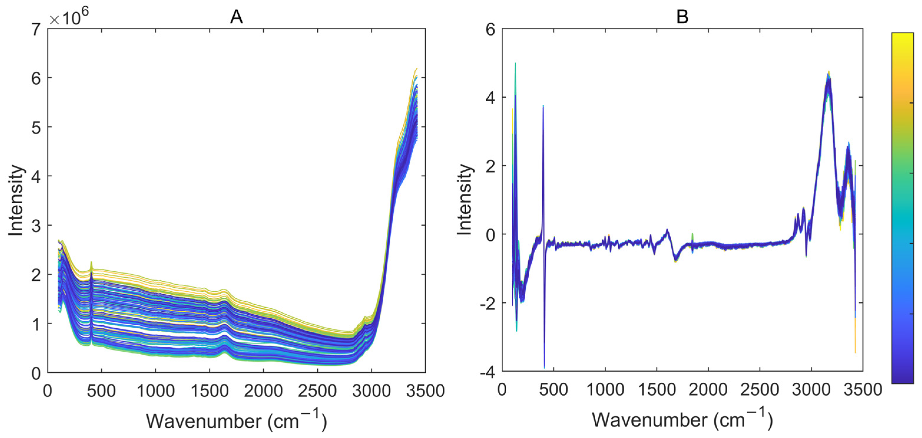
2.2. Data Acquisition

VCD determination was accomplished using the Countstar automated cell counter (Shanghai RuiYu Biotech Co. Ltd., Shanghai, China). Offline estimation of metabolite concentrations such as Gluc, Lac, and NH₄⁺ was carried out using the M900 SIEMAN biochemical analyzer (Shenzhen Siemantec Technology Co., Ltd., Shenzhen, China).

The acquisition of spectral data was facilitated by the multichannel Raman Rxn2 instrument (Endress+Hauser, Ann Arbor, MI, USA). This Raman system featured a CCD detector operating at −40 °C, a 785 nm excitation laser system (approximately 400 mW power), and two bIO-PRO-785 immersion probes (Endress+Hauser, Ann Arbor, MI, USA) connected to two stainless-steel bioreactors using holders (interface converting components). Before spectra collection, cosmic ray removal and dark current signal subtraction were performed using the Raman RunTime 6.3.1 (Kaiser Optical Systems, Ann Arbor, MI, USA). Each spectrum was obtained with an exposure time of 25 s and an averaging of 30 spectra. The collected spectral range encompassed 100–3425 cm⁻¹.

2.3. Variable Selection

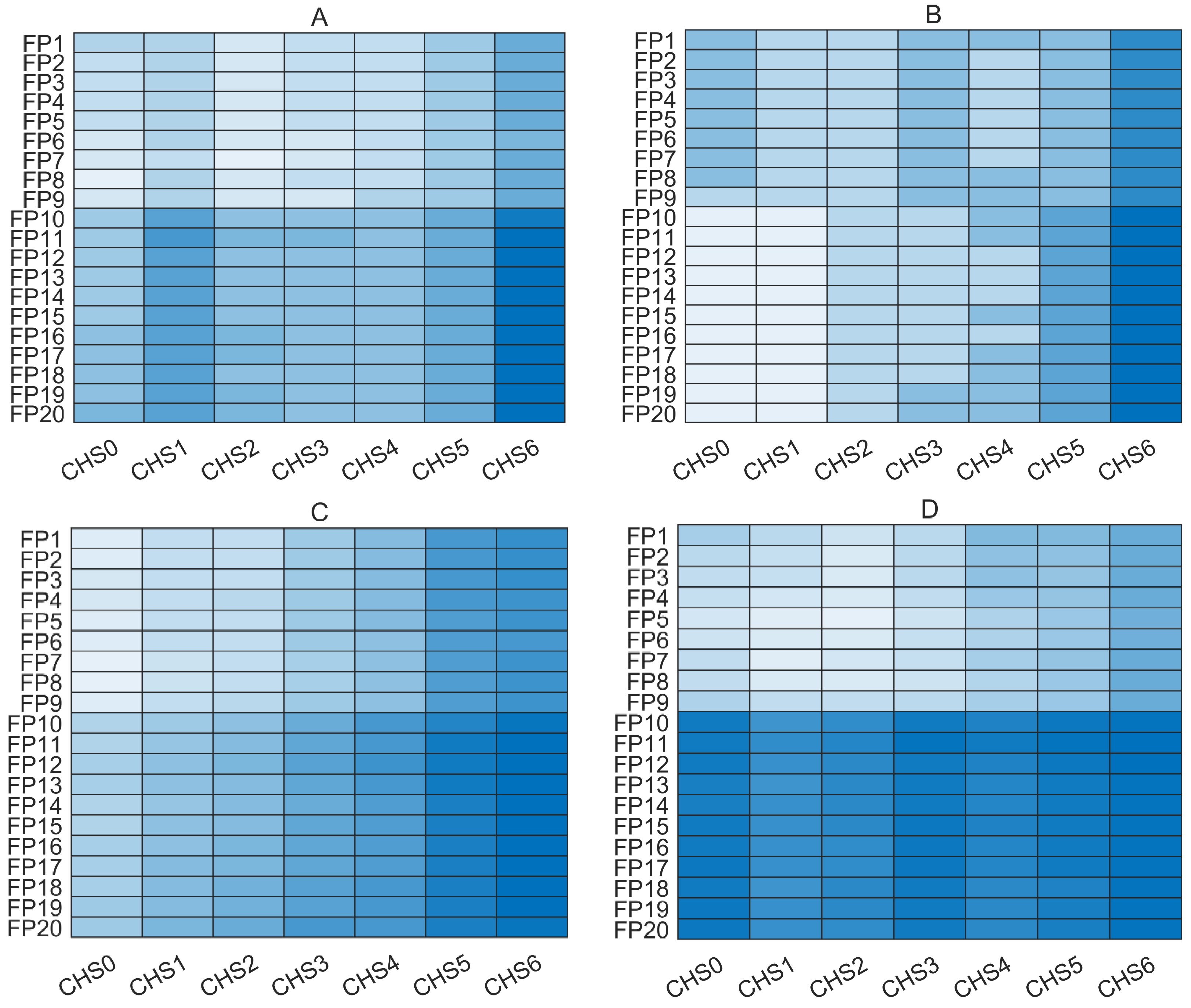
2.3.1. Spectral Regions Selection

We divided the Raman spectra into different regions for modeling to explore the impact of different spectral regions on the model’s performance. Twenty different spectral regions containing Raman fingerprint region were selected, labeled as FP1, FP2, FP3, FP4, FP5, FP6, FP7, FP8, FP9, FP10, FP11, FP12, FP13, FP14, FP15, FP16, FP17, FP18, FP19, and FP20, respectively. There are seven different spectral regions involving the C-H stretching region, labeled as CHS0, CHS1, CHS2, CHS3, CHS4, CHS5, and CHS6, respectively. The corresponding spectral ranges of each spectral region are shown in Figure 1. CHS0 does not contain any spectral variables, and FP20 plus CHS6 represents the whole range of spectra. The Raman-based models were developed by using different Raman fingerprint regions plus C-H stretching regions. In total, there were 7 × 20 = 140 different spectral regions used for modeling. These spectral regions involved different Raman fingerprint regions, Raman fingerprint regions plus C-H stretching regions, and the whole range of spectra, which could represent the spectral regions selected by most researchers.

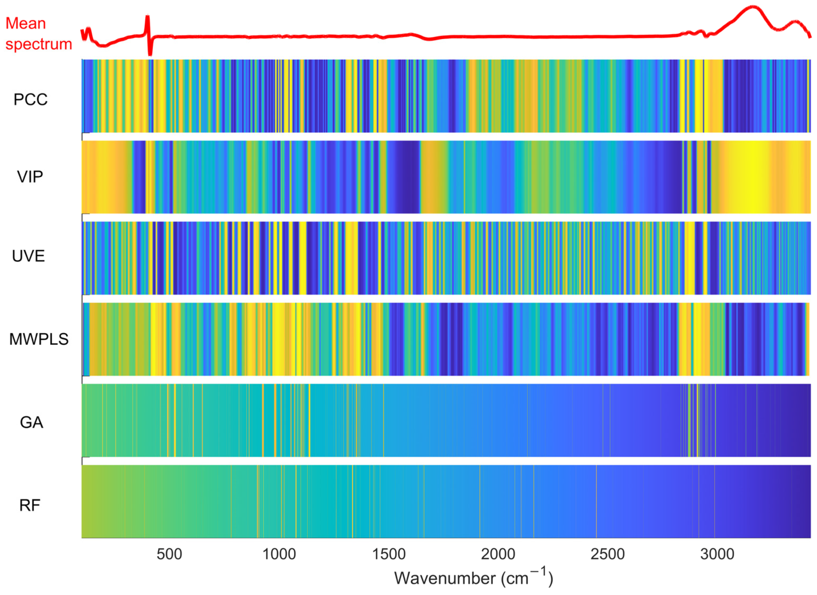
2.3.2. Variable Selection Algorithms

Different categories of variable selection algorithms, including PCC, VIP, UVE, MWPLS, GA, and RF, were used, and they can fully represent the variable selection algorithms currently in use.

PCC is straightforward and easy to understand. It calculates the correlation between the intensity vector, x, which corresponds to each spectral variable, and the concentration vector, y, of the analyzed component to obtain the correlation coefficient, r. Then, based on a given threshold, spectral variables with a correlation coefficient greater than this threshold are selected for model development [36]. The correlation coefficients for different components can vary significantly, and threshold values are not uniformly determined. In this study, the correlation coefficients were arranged in descending order, and spectral variables were selected according to a user-refined number.

The VIP method creates a weighted sum of the squares of the PLS model weights which leverages the amount of explained variance in each PLS latent variable [37]. In practice, this method produces a set of VIP scores for each Raman shift, reflecting its contribution to the variance in the concentration of each analyzed component. Generally, a variable is considered important if its VIP score is greater than 1.0. In this study, we selected a defined number of variables with VIP scores in descending order, regardless of this threshold.

The UVE method was developed to eliminate uninformative variables [38]. Artificial random variables are added to the data as a reference so that variables playing less important roles in the model than the random variables can be eliminated. Based on this definition of noise, UVE can eliminate non-informative variables. In this study, the Monte-Carlo UVE method is adopted, which is a type of method that has attracted increasing attention [39,40]. This method combines Monte-Carlo Sampling with PLS regression coefficient for spectral variable selection.

The iPLS method is used to divide intervals of equal width without overlapping, which may result in the loss of some variable information and reduce the optimization space for variable combination. The basic idea of the MWPLS method used in this study is to continuously move a window along the spectral axis. Each movement establishes a model through interactive verification [41], which is more effective than iPLS.

GA is a global optimization algorithm that learns from natural selection and genetic mechanisms in the biological world. It uses operators such as selection, crossover, and mutation to retain variables with better objective function values and eliminate poorer ones through continuous genetic iteration, ultimately achieving the optimal result [42]. Currently, GA has been widely used in the field of analytical chemistry, where it has yielded positive results in selecting characteristic variables [43].

The RF method refers to the paper published by Li et al. in 2013 [44]. It is a variable selection algorithm that offers different selection possibilities based on various variables and has demonstrated a strong performance in feature variable extraction in recent years. The method calculates the probability of each variable being selected through multiple iterations and selects the variable with a high preference probability as the feature variable.

To thoroughly evaluate the performance of various variable selection algorithms and investigate how different numbers of spectral variables impact model performance, we allowed each algorithm to select from the following numbers of variables: 1, 2, 3, 4, 5, 6, 7, 8, 9, 10, 20, 30, 40, 50, 60, 70, 80, 90, 100, 200, 300, 400, 500, 600, 700, 800, 900, 1000, 1100, 1200, 1300, 1400, 1500, 1600, 1700, 1800, 1900, 2000, 2100, 2200, 2300, 2400, 2500, 2600, 2700, 2800, 2900, 3000, 3100, 3200, and 3326 variables, respectively. The total number of spectral variables was 3326. As is well known, when the number of variables is small, each variable holds significant importance. However, when the number of variables is large, the importance of any single variable diminishes. Therefore, this selection range is reasonable and allows for a comprehensive evaluation of the performance of variable selection algorithms across different numbers of selected variables. It should be noted that although filter methods often select variables based on a defined threshold, variable selection algorithms used in this study select spectral variables based solely on the number of variables, without applying additional thresholds or criteria.

The parameters for the variable selection algorithms were set based on experience and references, and these parameters remained constant throughout the study. For MWPLS, the window width was set to 31. For MC-UVE, the number of Monte-Carlo simulations was set to 50, with the ratio of calibration samples to total samples at 0.6. For GA, the number of evaluations per run was 50. For RF, 500 simulations were run, and the initial number of variables was 500.

2.4. Model Calibration and Validation

Spectral preprocessing significantly influences the prediction performance of Raman models. Appropriate preprocessing methods are crucial in enhancing the signal-to-noise ratio and refining model precision. The typical preprocessing procedure used in Raman-based models for monitoring the cell culture process encompasses first derivative (15-point window) followed by standard normal variate (SNV) [7,8,17,18,21,23,26,29,45,46,47]. In this study, before the selection of spectral variables, Raman spectra were preprocessed by Savitzky–Golay first-order derivative (the width of window was 15, and the order of the polynomial was 2) to reduce baseline shift and enhance resolution. Then, SNV was employed for scattering correction.

Calibration models were established by PLS regression due to its widespread application in generating calibration models for cell culture monitoring [48]. Five-fold cross-validation was used to obtain root mean square error of cross-validation (RMSECV). The number of latent variables (LVs) was determined when RMSECV was the minimum. Studies have shown that the number of LVs selected by such a strategy is sometimes too large [49,50], resulting in overfitting of the model, so a rule was established (LV ≤ 15) to avert overfitting in our work. The performance of different variable selection strategies was evaluated using RMSECV from the initial 15 batches of data. The last batch (the sixteenth batch) was designated for validation to affirm the robustness of the optimized model. The performance of each model was assessed using root mean square error (RMSE) and correlation coefficient (R). Specifically, RMSEC represents the RMSE in calibration set, and RMSEP represents the RMSE in prediction set. R_C represents the R from calibration set, and R_P represents the R from prediction set. The performance improvement (PI) of Raman-based models is calculated according to Equation (1):

$$\mathrm{PI}\left(\%\right)={\displaystyle \frac{RMSE{P}^{before}-RMSE{P}^{after}}{RMSE{P}^{before}}}\times 100$$

(1)

where $RMSE{P}^{before}$ denotes the RMSEP of Raman-based models without spectral variable selection, and $RMSE{P}^{after}$ represents the RMSEP of Raman-based models with spectral variable selection.

The entire data processing was executed using MATLAB R2022b (MathWorks, Natick, MA, USA). Algorithms used in this study are from the libPLS 1.95 software package [51] and other in-house algorithms.

3. Results and Discussion

A total of sixteen batches of cell culture were conducted. The Raman spectra were aligned with offline reference values. After removing invalid values due to instrument failure, the number and concentration ranges of the collected samples are listed in

Table 2. The number and concentration information of the collected samples for glucose, lactate, viable cell density, and ammonium ion.

Component (Unit)	Batches 1–15			Batch 16
	n	Range	Mean ± SD	n	Range	Mean ± SD
Gluc (g/L)	173	1.50–4.18	2.42 ± 0.61	13	1.61–4.17	2.49 ± 0.68
Lac (g/L)	168	0.13–1.51	0.54 ± 0.36	13	0.18–0.78	0.35 ± 0.20
VCD (×106 cells/mL)	173	0.60–6.40	4.57 ± 1.59	13	0.75–6.06	4.65 ± 1.61
NH4+ (mmol/L)	169	2.67–15.39	9.91 ± 3.50	13	3.28–14.83	10.94 ± 4.14

n represents data size, and SD represents standard deviation.

. In chronological order, the first 15 batches were used to build the calibration model, while the last batch (the 16th batch) served as the external validation set.

3.1. Comparison of Different Spectral Regions

The 173 raw spectra and preprocessed spectra from the calibration set are presented in Figure 2. There was a significant baseline shift in the raw spectra, and peaks associated with concentration changes could not be directly observed. After the first derivative and SNV preprocessing, the baseline shift was removed, and the spectral signal-noise-ratio was promoted. The spectral intensity of 100–500 cm⁻¹ and 3000–3425 cm⁻¹ changes greatly. There are some small peaks during 500–3000 cm⁻¹, and the intensity change is relatively small. In fact, the regions with a wavenumber less than 1800 are all Raman fingerprint regions, the regions with a wavenumber of 1800–2800 are Raman-silent regions, and those with a wavenumber of 2800–3100 are C-H stretching regions [52,53]. It is difficult to choose the spectral regions for modeling directly from the spectra, and the judgment is subjective.

Models were constructed using various spectral regions, as outlined in Figure 1. The obtained RMSECV is depicted in Figure 3. The RMSECV obtained by the whole range of spectra (FP20 and CHS6 was used for modeling) for Gluc, Lac, VCD, and NH₄⁺ was 0.31 g/L, 0.13 g/L, 0.64 × 10⁶ cells/mL, and 1.15 mmol/L, respectively. Most of spectral regions selected in this study could effectively improve the prediction accuracy of Raman-based models, and the RMSECV was significantly reduced. However, spectral regions larger than 3200 cm⁻¹ may contain a large amount of noise, so the RMSECV is obtained using CHS5 or CHS6 larger. For Gluc, VCD, and NH₄⁺, when modeling with FP6-FP9, the obtained RMSECV is small; when modeling with FP10-FP20, the RMSECV is large, indicating that the regions of wavenumber <200 and 1800–2800 cm⁻¹ do not contain chemical information about Gluc, VCD, and NH₄⁺. The information involving molecular structure change is mostly contained in the spectral region of 200–1800 cm⁻¹. On the contrary, for Lac, the addition of regions smaller than 200 cm⁻¹ and Raman-silent regions (1800–2800 cm⁻¹) improved the model performance. For Gluc and NH₄⁺, the addition of the C-H stretching region improved the prediction accuracy of the Raman-based model to a certain extent. However, for VCD, the addition of C-H stretching regions degraded the model’s performance. The optimal model for Gluc, Lac, VCD, and NH₄⁺ was obtained when FP8 plus CHS0, FP17 plus CHS0, FP8 plus CHS0, and FP5 plus CHS2 were used for modeling, respectively, and the corresponding RMSECV was 0.18 g/L, 0.075 g/L, 0.39 × 10⁶ cells/mL, and 0.79 mmol/L.

The above results show that the commonly used spectral region selection can effectively reduce the prediction error of Raman-based models, but the optimal spectral region of each component is different. For Gluc, Lac, VCD, and NH₄⁺, the optimal spectral regions were 300–1800 cm⁻¹, 100–2500 cm⁻¹, 300–1800 cm⁻¹, and 600–1800 cm⁻¹ plus 2800–3000 cm⁻¹, respectively. These spectral regions were used to build models and predict the validation set, and the results are summarized in

Table 3. Calibration and prediction result of models with three different spectral regions.

Component	Spectral Region	N	LV	Calibration		Prediction		PI (%)
				RMSEC	RC	RMSEP	RP
Gluc	FP8 + CHS0	1500	9	0.11	0.98	0.18	0.97	17
	FP17 + CHS0	2400	14	0.09	0.99	0.17	0.97	20
	FP5 + CHS2	1400	7	0.13	0.98	0.14	0.98	34
Lac	FP8 + CHS0	1500	9	0.06	0.99	0.07	0.95	64
	FP17 + CHS0	2400	15	0.03	0.99	0.07	0.95	64
	FP5 + CHS2	1400	5	0.06	0.98	0.07	0.94	61
VCD	FP8 + CHS0	1500	8	0.28	0.98	0.25	0.99	48
	FP17 + CHS0	2400	12	0.29	0.98	0.41	0.98	13
	FP5 + CHS2	1400	9	0.27	0.99	0.26	0.99	44
NH4+	FP8 + CHS0	1500	7	0.55	0.99	0.61	0.99	30
	FP17 + CHS0	2400	12	0.47	0.99	0.66	0.99	24
	FP5 + CHS2	1400	7	0.50	0.99	0.52	0.99	39

N represents the number of selected variables.

. With the three selected spectral regions, the model performance was improved, and the R_C and R_P are both greater than 0.94. The model with spectral regions of 600–1800 cm⁻¹ plus 2800–3000 cm⁻¹ (FP5 + CHS2) was relatively better. The RMSEC and RMSEP obtained were closer, and the model performance was improved by 34–61%. Although these spectral regions can effectively improve the performance of Raman-based models, they are not very useful for simplifying the model. The number of selected spectral variables was greater than 1000.

3.2. Comparison of Different Variable Selection Algorithms

A well-designed variable selection algorithm has the potential to preserve model accuracy, simplify the model, and significantly enhance computational speed. Figure 4 elucidates the predictive outcomes achieved through the utilization of different numbers of variables for each variable selection algorithm. No matter which variable selection algorithm was used, when the number of selected variables was less than 10, the model error was large. When the number of selected variables was more than 1000, RMSECV changed less as the number of spectral variables changed. When the number of variables selected by VIP was less than 2700, the RMSECV obtained was larger than that of whole spectra, indicating that VIP could not effectively select spectral variables for Raman-based models in cell culture. GA, RF, and MWPLS could better improve the model performance for each component, and RF was better than GA and MWPLS. For RF, when the number of selected variables was less than 30, the RMSECV gradually decreased with the increase in the number of variables; when the number of selected variables was more than 30 and less than 300, the RMSECV was small and did not change much with the change in the number of spectral variables; and when the number of selected variables was more than 300, the RMSECV increased with the increase in the number of variables. GA was similar to RF, except that the RMSECV was generally higher than that obtained by RF. MWPLS tends to select a larger number of spectral variables to obtain a smaller RMSECV. The RMSECV obtained by UVE changed into an S-shape with the increase in the number of selected variables, and the RMSECV obtained was relatively small when the number of selected variables was from 300 to 1000. For PCC, when the number of selected variables was less than 40, the model prediction error was basically unchanged, with the increase in the number of selected variables; when the number of selected variables was 40–300, the model prediction error gradually decreased with the increase in the number of variables; and when the number of selected variables was greater than 300, the RMSECV obtained by the model had little difference.

Taking glucose for example, the ranking of spectral variables selected by these variable selection algorithms is plotted in Figure 5. The order of variables selected by different variable selection algorithms was quite different. PCC initially selected variables in the spectral ranges of 200–500 cm⁻¹ and 2800–3000 cm⁻¹ and then selected variables in the range of 1800–2500 cm⁻¹. The variables in the Raman fingerprint region were neglected. VIP selected variables at both ends of the spectrum (less than 500 cm⁻¹ and more than 3000 cm⁻¹), which severely affected the model performance. The spectral variables selected by UVE were relatively decentralized. Different spectral regions were involved even in the Raman-silent regions. The spectral variables selected by MWPLS were mainly in the Raman fingerprinting region and C-H stretching region. GA and RF were significantly different from other variable selection algorithms, and the selected spectral variables were so scattered that it was impossible to see the variable order.

In summary, the performance of variable selection algorithms is different. If an inappropriate variable selection algorithm was used, the performance of Raman-based models would be reduced. Therefore, the variable selection algorithm should be selected and used carefully. For the Raman-based models in the cell culture process, the above results show that RF and GA can significantly reduce the model prediction error, and the number of selected variables is from 30 to 300. The spectral variables selected by MWPLS are more reasonable than PCC, VIP, and UVE, and the model performance is improved to a certain extent. The number of spectral variables selected by MWPLS is large. The variables selected by PCC, VIP, and UVE cannot be explained, and the model performance is not ideal. When MWPLS was used to select 800, 2900, 800, and 100 variables for Gluc, Lac, VCD, and NH₄⁺, the minimum RMSECV obtained was 0.19 g/L, 0.092 g/L, 0.43 × 10⁶ cells/mL, and 0.92 mmol/L, respectively. When GA was used to select 100, 200, 300, and 90 variables for the four components, the minimum RMSECV obtained was 0.19 g/L, 0.082 g/L, 0.040 × 10⁶ cells/mL, and 0.73 mmol/L, respectively. When RF is used to select 80, 200, 60, and 100 variables for the four components, the minimum RMSECV obtained is 0.13 g/L, 0.051 g/L, 0.28 × 10⁶ cells/mL, and 0.48 mmol/L, respectively.

Table 4. Calibration and prediction results of models with three variable selection algorithms.

Component	Algorithm	N	LV	Calibration		Prediction		PI (%)
				RMSEC	RC	RMSEP	RP
Gluc	MWPLS	800	15	0.10	0.98	0.15	0.98	27
	GA	100	8	0.16	0.97	0.18	0.97	16
	RF	80	9	0.09	0.99	0.23	0.95	−8
Lac	MWPLS	2900	14	0.05	0.99	0.11	0.88	41
	GA	200	9	0.06	0.98	0.06	0.96	66
	RF	200	15	0.02	0.99	0.08	0.93	54
VCD	MWPLS	800	10	0.36	0.97	0.44	0.96	8
	GA	300	13	0.28	0.98	0.34	0.98	29
	RF	60	10	0.21	0.99	0.57	0.95	−21
NH4+	MWPLS	100	7	0.77	0.98	1.17	0.98	−36
	GA	90	13	0.56	0.99	0.69	0.99	20
	RF	100	10	0.29	0.99	0.70	0.99	19

N represents the number of selected variables.

listed the model calibration and prediction results of Gluc, Lac, VCD, and NH₄⁺, using MWPLS, GA, and RF variable selection algorithms. Although these variable selection algorithms could effectively reduce RMSECV according to the cross-validation results, not every model performance was improved for the external validation set. For example, the use of RF reduced model performance by 8% and 21% for glucose and viable cell density, respectively, and the use of MWPLS reduced model performance by 36% for ammonium ions. This may be caused by the large noise included in the selected variables.

According to Section 3.1, in order to select variables more effectively, some irrelevant and disturbed variables can be avoided by spectral region selection. We first defined the spectral region so that the variables were limited in the 600–1800 cm⁻¹ and 2800–3000 cm⁻¹ regions. Based on this, MWPLS, GA, and RF were used to select spectral variables, and the results of the model are shown in

Table 5. Calibration and prediction result of models with three variable selection algorithms after spectral region selection.

Component	Algorithm	N	LV	Calibration		Prediction		PI(%)
				RMSEC	RC	RMSEP	RP
Gluc	MWPLS	600	8	0.12	0.98	0.12	0.99	42
	GA	200	7	0.13	0.98	0.16	0.97	25
	RF	200	12	0.06	0.99	0.19	0.95	12
Lac	MWPLS	1300	5	0.08	0.98	0.07	0.93	60
	GA	100	7	0.06	0.98	0.05	0.97	73
	RF	300	12	0.03	0.99	0.06	0.95	65
VCD	MWPLS	1100	8	0.29	0.98	0.28	0.99	41
	GA	400	7	0.30	0.98	0.33	0.99	31
	RF	100	10	0.18	0.99	0.36	0.98	25
NH4+	MWPLS	1300	7	0.51	0.99	0.54	0.99	37
	GA	400	7	0.52	0.99	0.49	0.99	43
	RF	100	14	0.29	0.99	0.62	0.99	29

N represents the number of selected variables.

. After spectral region selection, MWPLS, GA, and RF effectively improved the model accuracy of each component. The R_C and R_P of all models was greater than 0.93. MWPLS improved the model performance by 37–60% by selecting 600–1300 variables. GA improved the model performance by 25–73% by selecting 100–400 variables. RF improved the model performance by 12–65% by selecting 100–300 variables.

The spectral region of 600–1800 cm⁻¹ and 2800–3000 cm⁻¹ is proved to improve the model performance in Section 3.1, but it does not mean that only this region can be used. In our view, MWPLS, GA, and RF can be used to effectively improve the model’s performance after some interfering variables are removed.

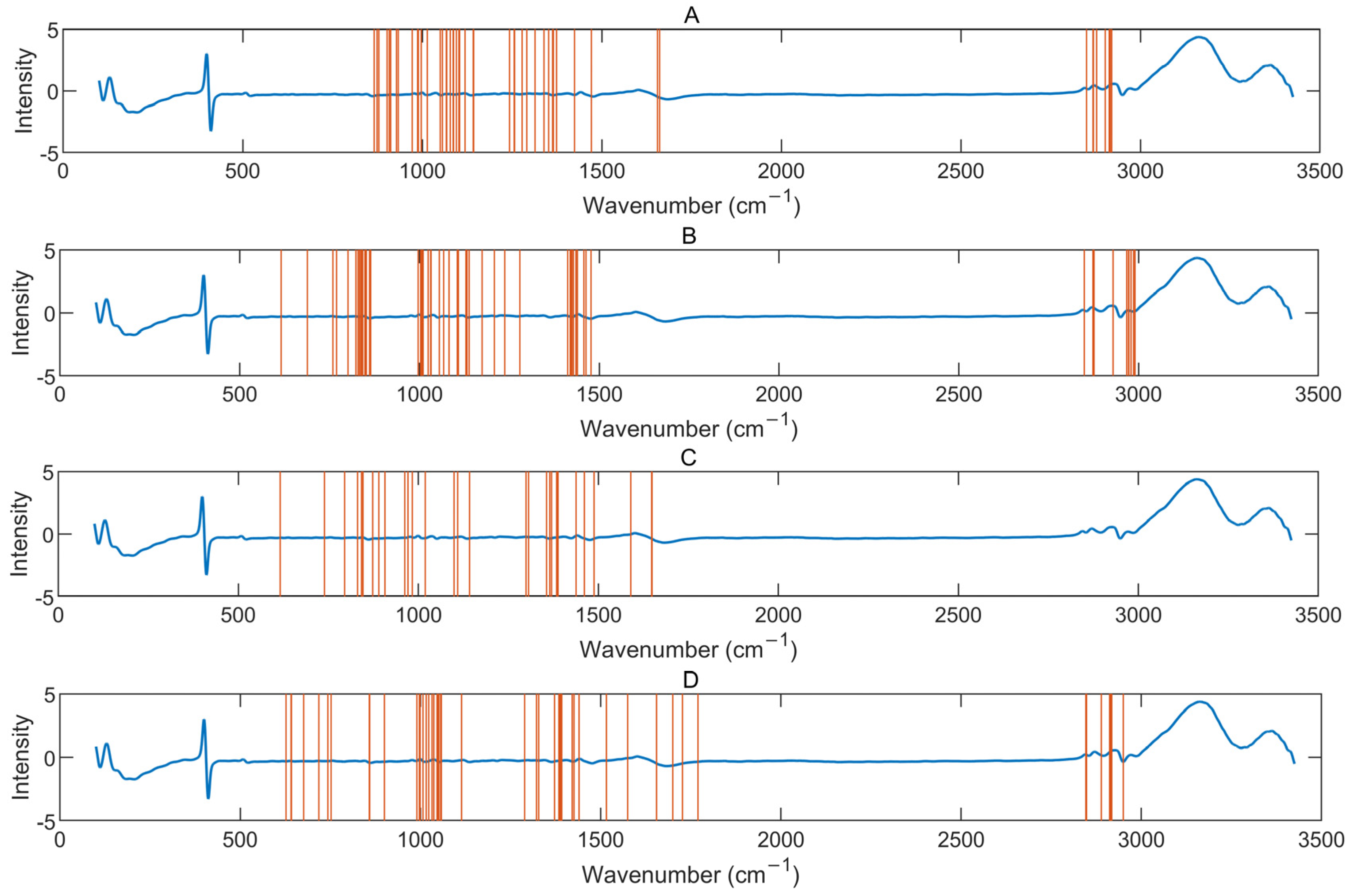
3.3. Combination of Variable Selection Algorithms

To further explore the impact of variable selection on model simplification and performance, we consider combining different variable selection algorithms. According to Table 4 and Table 5, MWPLS tends to select a larger number of variables, and RF tends to select a smaller number of variables. Therefore, three combination methods, MWPLS-GA, MWPLS-RF, and MWPLS-GA-RF, were proposed. Such combinations were used to reduce the number of variables and improve the model’s performance, and the results are listed in

Table 6. Calibration and prediction result of models with three combinations of variable selection algorithms after spectral region selection.

Component	Combination	N	LV	Calibration		Prediction		PI(%)
				RMSEC	RC	RMSEP	RP
Gluc	MWPLS-GA	200	5	0.16	0.97	0.19	0.96	10
	MWPLS-RF	70	12	0.09	0.99	0.12	0.99	43
	MWPLS-GA-RF	50	6	0.13	0.98	0.16	0.98	26
Lac	MWPLS-GA	100	5	0.07	0.98	0.06	0.95	66
	MWPLS-RF	90	14	0.04	0.99	0.10	0.87	47
	MWPLS-GA-RF	60	5	0.07	0.98	0.05	0.96	70
VCD	MWPLS-GA	100	6	0.34	0.98	0.26	0.99	46
	MWPLS-RF	200	10	0.17	0.99	0.44	0.96	7
	MWPLS-GA-RF	30	9	0.30	0.98	0.40	0.97	16
NH4+	MWPLS-GA	200	7	0.52	0.99	0.52	0.99	40
	MWPLS-RF	200	12	0.25	0.99	0.79	0.99	8
	MWPLS-GA-RF	50	8	0.47	0.99	0.58	0.99	33

N represents the number of selected variables.

. It should be noted that all variable selection algorithms were used after spectral regions 600–1800 cm⁻¹ and 2800–3000 cm⁻¹ were selected. MWPLS-GA improved the model performance by 10–66% by selecting 100–200 variables. MWPLS-RF improved the model performance by 7–47% by selecting 70–200 variables. MWPLS-GA-RF improved the model performance by 16–70% by selecting 30–60 variables. The combination of variable selection algorithms can effectively reduce the number of selected variables, while ensuring the performance of the model. MWPLS-GA-RF especially improved the model performance by selecting less than 100 variables, which could promote the application of Raman spectroscopy in the cell culture process. For MWPLS-GA and MWPLS-RF, the number of selected variables was relatively large, and the model performance improvement was limited. Compared with the results of GA and RF, the results of MWPLS-GA and MWPLS-RF were unsatisfactory.

The spectral variables selected by MWPLS-GA-RF are plotted in Figure 6. For glucose, the selected spectral variables are mainly located at 850–1150 cm⁻¹, 1250–1500 cm⁻¹, and 2850–2950 cm⁻¹, which are related to $\nu$(C-O) and $\nu$(C-C) stretches (1000–1200 cm⁻¹); $\delta$(CH₂) and $\delta$(CH₂OH) deformations (1300–1500 cm⁻¹); $\delta$(C-OH), $\delta$(C-CH), and $\delta$(O-CH) side-group deformations (800–950 cm⁻¹); $\nu$(C-O) and $\nu$(C-C) stretches (950–1200 cm⁻¹); and $\delta$(CH₂) and $\delta$(CH₂OH) deformations (1250–1500 cm⁻¹) [54]. For lactate, the selected spectral variables are mainly located at 600–900 cm⁻¹, 1000–1300 cm⁻¹, 1400–1500 cm⁻¹, and 2800–3000 cm⁻¹. According to the literature [55], the characteristic spectral regions of lactate were 640–660 cm⁻¹, 720–775 cm⁻¹, 855 cm⁻¹, 930 cm⁻¹, and 2900–2980 cm⁻¹, involving C-COH deformations, C-CO₂- stretches, C-COO- stretching, CH₃ rocking, and CH₃ stretching vibrations. The spectral variables selected for viable cell density are mainly located between 800 cm⁻¹ and 1500 cm⁻¹, which are related to C-C stretch modes (926–975 cm⁻¹), the C-N vibration mode of lipids and proteins (1076 cm⁻¹), C-O vibration mode of carbohydrates (1125 cm⁻¹), and the ring breathing mode of adenine and guanine nucleobases in DNA and RNA (1326–1475 cm⁻¹) [21]. The spectral variables of ammonium ion are mainly located in 600–800 cm⁻¹, 1000–1100 cm⁻¹, 1300–1500 cm⁻¹, and 2800–3000 cm⁻¹, which are similar to the report [9]. Although Raman spectroscopy does not provide direct structural variation information about ammonium ion, it can still provide better prediction results through indirect relation. In addition, the selection of C-H stretching regions was consistent with the results in Section 3.1. Except for viable cell density, the addition of C-H stretching regions could improve the model’s performance. All of these indicate that the variables selected by MWPLS-GA-RF are reasonable.

The cell culture process was monitored in real time using the model constructed with the spectral variables selected by MWPLS-GA-RF. As shown in Figure 7, the models effectively projected the concentrations of these four components and captured the perturbations induced by additional medium feeding. Compared with the monitoring performance using the whole range of spectra (no selection of spectral variable), the prediction of the model with MWPLS-GA-RF was less noisy and closer to the reference value.

In summary, the combination of two variable selection algorithms performed similarly to single variable selection algorithms, failing to further improve model accuracy or reduce the number of selected variables. In contrast, the combination of three variable selection algorithms was able to select fewer variables for modeling, and the selected variables were reasonable. The variables selected by MWPLS-GA-RF were used to construct the model, and the model’s performance was satisfactory. When the model was used for real-time monitoring of the cell culture process, the concentration changes in components in the bioreactor were accurately depicted.

In previous work [35], the optimal RMSEP values for glucose, lactate, and viable cell density were 0.22 g/L, 0.08 g/L, and 0.31 × 10⁶ cells/mL, respectively, and the number of spectral variables for each component was over 1000. In this study, the RMSEP was significantly reduced by selecting spectral variables based on MWPLS-GA. Using the variable selection method MWPLS-GA-RF with the number of variables < 100, the RMSEP values obtained for glucose, lactate, and viable cell density were 0.16 g/L, 0.05 g/L, and 0.40 × 10⁶ cells/mL, respectively, which is an improvement over the results from previous work.

It is important to note that researchers may have different objectives, such as improving model performance or simplifying the model, which can lead to variations in the definition of the optimal variable selection strategy. The combination method of MWPLS-GA-RF has been shown to enhance model performance, while effectively simplifying the model. However, if dimensionality reduction is not required, simpler approaches, such as spectral region selection (e.g., 600–1800 cm⁻¹ plus 2800–3000 cm⁻¹) or single variable selection algorithms (e.g., GA and RF), can also effectively improve the model’s performance. Model robustness is a key issue that needs to be addressed during the variable selection process, especially when fewer variables are chosen. In this study, the calibration set was used for cross-validation, and the external validation set was then used to assess the model’s performance, which provided some assurance of model robustness. However, if the model is to be used in real production, more detailed robustness studies are required. For example, more external validation sets should be used to test the model further. In addition, the data in this study were collected from the fed-batch culture of CHO-S cells. To ensure broader applicability, it would be beneficial to include more cases, such as the culture of CHO-K1 cells and perfusion culture, to confirm the applicability of MWPLS-GA-RF.

4. Conclusions

Variable selection is often grounded in a foundational understanding of the spectral properties of samples when the components are simple and the characteristic peaks of the spectrum are evident. However, leveraging mathematical strategies for variable selection proves to be more effective in complex samples. In this study, it was found that the commonly used spectral regions could enhance model performance for different analyzed components; however, their effect on simplifying the model was not significant. The spectral region of 600–1800 cm⁻¹ combined with 2800–3000 cm⁻¹ improved model performance by 34–64% by selecting 1400 spectral variables. The variables selected by PCC, UVE, and VIP were not reasonable, resulting in poor model performance across all components. MWPLS, GA, and RF demonstrated better applicability, but they should be employed only after selecting the appropriate spectral regions. The combination of two variable selection algorithms was unsatisfactory, yielding a performance similar to that of a single variable selection algorithm. In contrast, the combination of three variable selection algorithms (MWPLS-GA-RF) successfully selected fewer variables for modeling, and the selected variables were deemed reasonable. For Gluc, Lac, VCD, and NH₄⁺, the model performance improved by 16–70% when applying MWPLS-GA-RF with the selection of 30–60 variables. With the optimal variable selection strategy, monitoring can be effectively performed, providing guidance for researchers on variable selection and promoting the application of Raman spectroscopy in cell culture processes.

References

1. Goh, J.B.; Ng, S.K. Impact of host cell line choice on glycan profile. Crit. Rev. Biotechnol. 2018, 38, 851–867. [Google Scholar] [CrossRef] [PubMed]
2. Sidoli, F.R.; Mantalaris, A.; Asprey, S.P. Modelling of Mammalian Cells and Cell Culture Processes. Cytotechnology 2004, 44, 27–46. [Google Scholar] [CrossRef]
3. Jin, S.; Sun, F.; Hu, Z.; Li, Y.; Zhao, Z.; Du, G.; Shi, G.; Chen, J. Online quantitative substrate, product, and cell concentration in citric acid fermentation using near-infrared spectroscopy combined with chemometrics. Spectrochim. Acta Part A 2023, 285, 121842. [Google Scholar] [CrossRef] [PubMed]
4. Abu-Absi, N.R.; Kenty, B.M.; Cuellar, M.E.; Borys, M.C.; Sakhamuri, S.; Strachan, D.J.; Hausladen, M.C.; Li, Z.J. Real time monitoring of multiple parameters in mammalian cell culture bioreactors using an in-line Raman spectroscopy probe. Biotechnol. Bioeng. 2011, 108, 1215–1221. [Google Scholar] [CrossRef]
5. Webster, T.A.; Hadley, B.C.; Hilliard, W.; Jaques, C.; Mason, C. Development of generic Raman models for a GS-KOTM CHO platform process. Biotechnol. Prog. 2018, 34, 730–737. [Google Scholar] [CrossRef] [PubMed]
6. Tulsyan, A.; Schorner, G.; Khodabandehlou, H.; Wan, T.; Coufal, M.; Undey, C. A machine-learning approach to calibrate generic Raman models for real-time monitoring of cell culture processes. Biotechnol. Bioeng. 2019, 116, 2575–2586. [Google Scholar] [CrossRef]
7. Webster, T.A.; Hadley, B.C.; Dickson, M.; Busa, J.K.; Jaques, C.; Mason, C. Feedback control of two supplemental feeds during fed-batch culture on a platform process using inline Raman models for glucose and phenylalanine concentration. Bioprocess Biosyst. Eng. 2021, 44, 127–140. [Google Scholar] [CrossRef]
8. Eyster, T.; Talwar, S.; Fernandez, J.; Foster, S.; Hayes, J.; Allen, R.; Reidinger, S.; Wan, B.; Ji, X.; Aon, J.; et al. Tuning monoclonal antibody galactosylation using Raman spectroscopy-controlled lactic acid feeding. Biotechnol. Progr. 2021, 37, e3085. [Google Scholar] [CrossRef]
9. Chen, G.; Hu, J.; Qin, Y.; Zhou, W. Viable cell density on-line auto-control in perfusion cell culture aided by in-situ Raman spectroscopy. Biochem. Eng. J. 2021, 172, 108063. [Google Scholar] [CrossRef]
10. Wasalathanthri, D.P.; Rehmann, M.S.; Song, Y.; Gu, Y.; Mi, L.; Shao, C.; Chemmalil, L.; Lee, J.; Ghose, S.; Borys, M.C.; et al. Technology outlook for real-time quality attribute and process parameter monitoring in biopharmaceutical development—A review. Biotechnol. Bioeng. 2020, 117, 3182–3198. [Google Scholar] [CrossRef] [PubMed]
11. Koch, M.; Suhr, C.; Roth, B.; Meinhardt-Wollweber, M. Iterative morphological and mollifier-based baseline correction for Raman spectra. J. Raman Spectrosc. 2017, 48, 336–342. [Google Scholar] [CrossRef]
12. Lieber, C.A.; Mahadevan-Jansen, A. Automated method for subtraction of fluorescence from biological Raman spectra. Appl. Spectrosc. 2003, 57, 1363–1367. [Google Scholar] [CrossRef]
13. Jiang, H.; Xu, W.; Ding, Y.; Chen, Q. Quantitative analysis of yeast fermentation process using Raman spectroscopy: Comparison of CARS and VCPA for variable selection. Spectrochim. Acta Part A 2020, 228, 117781. [Google Scholar] [CrossRef]
14. Classen, J.; Aupert, F.; Reardon, K.F.; Solle, D.; Scheper, T. Spectroscopic sensors for in-line bioprocess monitoring in research and pharmaceutical industrial application. Anal. Bioanal. Chem. 2017, 409, 651–666. [Google Scholar] [CrossRef]
15. Kamruzzaman, M.; Kalita, D.; Ahmed, M.T.; ElMasry, G.; Makino, Y. Effect of variable selection algorithms on model performance for predicting moisture content in biological materials using spectral data. Anal. Chim. Acta 2022, 1202, 339390. [Google Scholar] [CrossRef]
16. Rafferty, C.; Johnson, K.; O’Mahony, J.; Burgoyne, B.; Rea, R.; Balss, K.M. Analysis of chemometric models applied to Raman spectroscopy for monitoring key metabolites of cell culture. Biotechnol. Progr. 2020, 36, e2977. [Google Scholar] [CrossRef]
17. Schwarz, H.; Mäkinen, M.E.; Castan, A.; Chotteau, V. Monitoring of amino acids and antibody N-glycosylation in high cell density perfusion culture based on Raman spectroscopy. Biochem. Eng. J. 2022, 182, 108426. [Google Scholar] [CrossRef]
18. Petillot, L.; Pewny, F.; Wolf, M.; Sanchez, C.; Thomas, F.; Sarrazin, J.; Fauland, K.; Katinger, H.; Javalet, C.; Bonneville, C. Calibration transfer for bioprocess Raman monitoring using Kennard Stone piecewise direct standardization and multivariate algorithms. Eng. Rep. 2020, 2, e12230. [Google Scholar] [CrossRef]
19. Matthews, T.E.; Berry, B.N.; Smelko, J.; Moretto, J.; Moore, B.; Wiltberger, K. Closed loop control of lactate concentration in mammalian cell culture by Raman spectroscopy leads to improved cell density, viability, and biopharmaceutical protein production. Biotechnol. Bioeng. 2016, 113, 2416–2424. [Google Scholar] [CrossRef]
20. Santos, R.M.; Kaiser, P.; Menezes, J.C.; Peinado, A. Improving reliability of Raman spectroscopy for mAb production by upstream processes during bioprocess development stages. Talanta 2019, 199, 396–406. [Google Scholar] [CrossRef]
21. André, S.; Lagresle, S.; Hannas, Z.; Calvosa, É.; Duponchel, L. Mammalian cell culture monitoring using in situ spectroscopy: Is your method really optimised? Biotechnol. Progr. 2017, 33, 308–316. [Google Scholar] [CrossRef]
22. Domján, J.; Pantea, E.; Gyürkés, M.; Madarász, L.; Kozák, D.; Farkas, A.; Horváth, B.; Benkő, Z.; Nagy, Z.K.; Marosi, G.; et al. Real-time amino acid and glucose monitoring system for the automatic control of nutrient feeding in CHO cell culture using Raman spectroscopy. Biotechnol. J. 2022, 17, 2100395. [Google Scholar] [CrossRef] [PubMed]
23. André, S.; Lagresle, S.; Da Sliva, A.; Heimendinger, P.; Hannas, Z.; Calvosa, É.; Duponchel, L. Developing global regression models for metabolite concentration prediction regardless of cell line: Developing global regression models. Biotechnol. Bioeng. 2017, 114, 2550–2559. [Google Scholar] [CrossRef]
24. Rafferty, C.; O’Mahony, J.; Rea, R.; Burgoyne, B.; Balss, K.M.; Lyngberg, O.; O’Mahony-Hartnett, C.; Hill, D.; Schaefer, E. Raman spectroscopic based chemometric models to support a dynamic capacitance based cell culture feeding strategy. Bioprocess Biosyst. Eng. 2020, 43, 1415–1429. [Google Scholar] [CrossRef] [PubMed]
25. Tulsyan, A.; Wang, T.; Schorner, G.; Khodabandehlou, H.; Coufal, M.; Undey, C. Automatic real-time calibration, assessment, and maintenance of generic Raman models for online monitoring of cell culture processes. Biotechnol. Bioeng. 2020, 117, 406–416. [Google Scholar] [CrossRef]
26. Liu, Z.; Zhang, Z.; Qin, Y.; Chen, G.; Hu, J.; Wang, Q.; Zhou, W. The application of Raman spectroscopy for monitoring product quality attributes in perfusion cell culture. Biochem. Eng. J. 2021, 173, 108064. [Google Scholar] [CrossRef]
27. Mehmood, T.; Liland, K.H.; Snipen, L.; Sæbø, S. A review of variable selection methods in Partial Least Squares Regression. Chemom. Intell. Lab. Syst. 2012, 118, 62–69. [Google Scholar] [CrossRef]
28. Yun, Y.-H.; Li, H.-D.; Deng, B.-C.; Cao, D.-S. An overview of variable selection methods in multivariate analysis of near-infrared spectra. TTrAC Trends Anal. Chem. 2019, 113, 102–115. [Google Scholar] [CrossRef]
29. Santos, R.M.; Kessler, J.-M.; Salou, P.; Menezes, J.C.; Peinado, A. Monitoring mAb cultivations with in-situ raman spectroscopy: The influence of spectral selectivity on calibration models and industrial use as reliable PAT tool. Biotechnol. Progr. 2018, 34, 659–670. [Google Scholar] [CrossRef] [PubMed]
30. Wang, B.; He, J.; Zhang, S.; Li, L. Nondestructive prediction and visualization of total flavonoids content in Cerasus Humilis fruit during storage periods based on hyperspectral imaging technique. J. Food Process Eng. 2021, 44, e13807. [Google Scholar] [CrossRef]
31. Yu, H.-D.; Yun, Y.-H.; Zhang, W.; Chen, H.; Liu, D.; Zhong, Q.; Chen, W.; Chen, W. Three-step hybrid strategy towards efficiently selecting variables in multivariate calibration of near-infrared spectra. Spectrochim. Acta Part A Mol. Biomol. Spectrosc. 2020, 224, 117376. [Google Scholar] [CrossRef] [PubMed]
32. Variable selection in near-infrared spectroscopy: Benchmarking of feature selection methods on biodiesel data. Anal. Chim. Acta 2011, 692, 63–72. [CrossRef] [PubMed]
33. Li, P.; Ma, J.; Zhong, N. Raman spectroscopy combined with support vector regression and variable selection method for accurately predicting salmon fillets storage time. Optik 2021, 247, 167879. [Google Scholar] [CrossRef]
34. Zhao, F.; Wan, Y.; Nie, L.; Jiao, J.; Gao, D.; Sun, Y.; Chen, Z.; Shi, Y.; Yang, J.; Pan, J.; et al. 1 H NMR-based process understanding and biochemical marker identification methodology for monitoring CHO cell culture process during commercial-scale manufacturing. Biotechnol. J. 2023, 18, e2200616. [Google Scholar] [CrossRef] [PubMed]
35. Yan, X.; Dong, X.; Wan, Y.; Gao, D.; Chen, Z.; Zhang, Y.; Zheng, Z.; Chen, K.; Jiao, J.; Sun, Y.; et al. Development of an in-line Raman analytical method for commercial-scale CHO cell culture process monitoring: Influence of measurement channels and batch number on model performance. Biotechnol. J. 2023, 19, e2300395. [Google Scholar] [CrossRef] [PubMed]
36. Cheng, J.; Chen, Z.; Yi, S. Wavelength selection algorithm based on minium correlation coefficient for multivariate calibartion. Spectrosc. Spectr. Anal. 2022, 42, 719–725. [Google Scholar] [CrossRef]
37. Farrés, M.; Platikanov, S.; Tsakovski, S.; Tauler, R. Comparison of the variable importance in projection (VIP) and of the selectivity ratio (SR) methods for variable selection and interpretation. J. Chemom. 2015, 29, 528–536. [Google Scholar] [CrossRef]
38. Centner, V.; Massart, D.-L.; De Noord, O.E.; De Jong, S.; Vandeginste, B.M.; Sterna, C. Elimination of Uninformative Variables for Multivariate Calibration. Anal. Chem. 1996, 68, 3851–3858. [Google Scholar] [CrossRef] [PubMed]
39. Han, Q.-J.; Wu, H.-L.; Cai, C.-B.; Xu, L.; Yu, R.-Q. An ensemble of Monte Carlo uninformative variable elimination for wavelength selection. Anal. Chim. Acta 2008, 612, 121–125. [Google Scholar] [CrossRef] [PubMed]
40. Niu, X.; Zhao, Z.; Jia, K.; Li, X. A feasibility study on quantitative analysis of glucose and fructose in lotus root powder by FT-NIR spectroscopy and chemometrics. Food Chem. 2012, 133, 592–597. [Google Scholar] [CrossRef] [PubMed]
41. Jiang, J.-H.; Berry, R.J.; Siesler, H.W.; Ozaki, Y. Wavelength Interval Selection in Multicomponent Spectral Analysis by Moving Window Partial Least-Squares Regression with Applications to Mid-Infrared and Near-Infrared Spectroscopic Data. Anal. Chem. 2002, 74, 3555–3565. [Google Scholar] [CrossRef] [PubMed]
42. Jouan-Rimbaud, D.; Massart, D.-L.; Leardi, R.; De Noord, O.E. Genetic Algorithms as a Tool for Wavelength Selection in Multivariate Calibration. Anal. Chem. 1995, 67, 4295–4301. [Google Scholar] [CrossRef]
43. Leardi, R. Application of genetic algorithm-PLS for feature selection in spectral data sets. J. Chemom. 2000, 14, 643–655. [Google Scholar] [CrossRef]
44. Yun, Y.-H.; Li, H.-D.; Wood, L.R.E.; Fan, W.; Wang, J.-J.; Cao, D.-S.; Xu, Q.-S.; Liang, Y.-Z. An efficient method of wavelength interval selection based on random frog for multivariate spectral calibration. Spectrochim. Acta Part A Mol. Biomol. Spectrosc. 2013, 111, 31–36. [Google Scholar] [CrossRef] [PubMed]
45. Bhatia, H.; Mehdizadeh, H.; Drapeau, D.; Yoon, S. In-line monitoring of amino acids in mammalian cell cultures using Raman spectroscopy and multivariate chemometrics models. Eng. Life Sci. 2018, 18, 55–61. [Google Scholar] [CrossRef] [PubMed]
46. Liu, Y.-J.; André, S.; Saint Cristau, L.; Lagresle, S.; Hannas, Z.; Calvosa, É.; Devos, O.; Duponchel, L. Multivariate statistical process control (MSPC) using Raman spectroscopy for in-line culture cell monitoring considering time-varying batches synchronized with correlation optimized warping (COW). Anal. Chim. Acta 2017, 952, 9–17. [Google Scholar] [CrossRef] [PubMed]
47. Berry, B.; Moretto, J.; Matthews, T.; Smelko, J.; Wiltberger, K. Cross-scale predictive modeling of CHO cell culture growth and metabolites using Raman spectroscopy and multivariate analysis. Biotechnol. Progr. 2015, 31, 566–577. [Google Scholar] [CrossRef]
48. Zavala-Ortiz, D.A.; Denner, A.; Aguilar-Uscanga, M.G.; Marc, A.; Ebel, B.; Guedon, E. Comparison of partial least square, artificial neural network, and support vector regressions for real-time monitoring of CHO cell culture processes using in situ near-infrared spectroscopy. Biotechnol. Bioeng. 2022, 119, 535–549. [Google Scholar] [CrossRef] [PubMed]
49. Hubli, G.B.; Banerjee, S.; Rathore, A.S. Near-infrared spectroscopy based monitoring of all 20 amino acids in mammalian cell culture broth. Talanta 2023, 254, 124187. [Google Scholar] [CrossRef]
50. Tanemura, H.; Kitamura, R.; Yamada, Y.; Hoshino, M.; Kakihara, H.; Nonaka, K. Comprehensive modeling of cell culture profile using Raman spectroscopy and machine learning. Sci. Rep. 2023, 13, 21805. [Google Scholar] [CrossRef]
51. Li, H.-D.; Xu, Q.-S.; Liang, Y.-Z. libPLS: An integrated library for partial least squares regression and linear discriminant analysis. Chemom. Intell. Lab. Syst. 2018, 176, 34–43. [Google Scholar] [CrossRef]
52. Yin, Y.; Li, Q.; Ma, S.; Liu, H.; Dong, B.; Yang, J.; Liu, D. Prussian Blue as a Highly Sensitive and Background-Free Resonant Raman Reporter. Anal. Chem. 2017, 89, 1551–1557. [Google Scholar] [CrossRef] [PubMed]
53. Yu, Y.; Wang, Y.; Lin, K.; Zhou, X.; Liu, S.; Sun, J. New spectral assignment of n-propanol in the C―H stretching region. J. Raman Spectrosc. 2016, 47, 1385–1393. [Google Scholar] [CrossRef]
54. De Gelder, J.; De Gussem, K.; Vandenabeele, P.; Moens, L. Reference database of Raman spectra of biological molecules. J. Raman Spectrosc. 2007, 38, 1133–1147. [Google Scholar] [CrossRef]
55. Pecul, M.; Rizzo, A.; Leszczynski, J. Vibrational Raman and Raman Optical Activity Spectra of d-Lactic Acid, d-Lactate, and d-Glyceraldehyde:  Ab Initio Calculations. J. Phys. Chem. A 2002, 106, 11008–11016. [Google Scholar] [CrossRef]
Figure 1. Different spectral regions selected for modeling.
Applsci 14 08890 g001
Figure 2. Raw spectra (A) and spectra preprocessed by first derivative and SNV (B). Color changes from yellow to blue represent the beginning to the end of cell culture.
Applsci 14 08890 g002
Figure 3. Model cross-validation results using different spectral regions. (A) Glucose, (B) lactate, (C) viable cell density, and (D) ammonium ion. The darker blue represents the larger RMSECV.
Applsci 14 08890 g003
Figure 4. Model cross-validation results with different numbers of variables selected by six variable selection algorithms. (A) Glucose, (B) lactate, (C) viable cell density, and (D) ammonium ion.
Applsci 14 08890 g004
Figure 5. Ranking of variables selected by different variable selection algorithms. The color changing from yellow to green to blue represents the decreasing order of spectral variable selected by variable selection algorithms. Specifically, yellow indicates the top variable, and blue indicates the bottom variable.
Applsci 14 08890 g005
Figure 6. Spectral variables selected by MWPLS-GA-RF. (A) Glucose, (B) lactate, (C) viable cell density, and (D) ammonium ion. A mean spectrum after preprocessing was used to show the selected variables.
Applsci 14 08890 g006
Figure 7. Monitoring for glucose (A), lactate (B), viable cell density (C), and ammonium ion (D).
Applsci 14 08890 g007