Consensus Control of Leader–Follower Multi-Agent Systems with Unknown Parameters and Its Circuit Implementation

Abstract

With the development and progress of Internet and data technology, the consensus control of multi-agent systems has been an important topic in nonlinear science. How to effectively achieve the consensus of leader–follower multi-agent systems at a low cost is a difficult problem. This paper analyzes the consensus control of complex financial systems. Firstly, the dynamic characteristics of the financial system are analyzed by the equilibrium points, bifurcation diagrams, and Lyapunov exponent spectra. The behavior of the financial system is discussed by different parameter values. Secondly, according to the Lyapunov stability theorem, the consensus of master–slave systems is proposed by linear feedback control, wherein the controllers are simple and low cost. And an adaptive control method for the consensus of master–slave systems is investigated based on financial systems with unknown parameters. In theory, the consensus of the leader–follower multi-agent systems is proved by the parameter identification laws and linear feedback control method. Finally, the effectiveness and reliability of the consensus of leader–follower multi-agent systems are verified through the experimental simulation results and circuit implementation.

1. Introduction

There are many consensus phenomena in nature such as bird and fish clusters, and they are actually related to the consensus control problem of multi-agent systems. In recent years, the consensus problem of intelligent agents is one of important topics in nonlinear science. With the development of the Internet, big data technology, and artificial intelligence science, more possibilities are being provided for consensus control and practical application. How to control the behavior of multi-agent systems to achieve a predetermined or synchronized trajectory is an important topic, such as the consensus of unmanned aerial vehicles, robotic arms, aircraft, etc. Chaos is also one of the interesting phenomena in nonlinear science, and it has attracted much attention due to its high sensitivity to initial values and the complexity of its motion trajectory [1,2,3,4,5,6]. Some potential applications have been studied based on chaotic systems, such as finance model analysis [7,8], circuit implementation [9], chaos-based encryption [10,11,12], and secure communication [13,14]. In order to verify the effectiveness and feasibility of control methods for tracking or synchronizing complex behavior, chaotic systems can usually be used to simulate the motion trajectory of intelligent agents.

Many control methods have been proposed for the consensus or synchronization of complex dynamical systems, such as feedback control [15], active control [16,17], adaptive control [18,19], event-triggered control [20], pulse control [21,22], etc. In reference [23], an introduction to event-triggered coordination for multi-agent average consensus was investigated using the motivations of event-triggered strategies for consensus, methods for algorithm synthesis, technical challenges, and their applications in distributed control. In reference [24], the master–slave synchronization of a type of the complex-valued chaotic Lur’e systems with time delay was addressed with decomposing complex-valued dynamic systems into two real-valued systems. A nonlinear active controller was obtained to synchronize the two identical dissipative fermionic systems in their chaotic states for different initial values [17]. The role of different structures of coupling terms on the synchronization properties of master–slave chaotic system configurations was investigated based on the Lyapunov theory for linear systems with nonlinear vanishing perturbations [25]. Sufficient conditions for master–slave synchronization of Lur’e systems are presented for a known time delay in the master and slave systems [26]. In reference [27], the position control of a master–slave synchronization robotic arm driven by a D.C. motor using a PID (Proportional, Integral, and Derivative) controller with software and hardware design was analyzed. The sufficient conditions for the quasi-consensus of multi-agent systems were studied via event-triggered impulsive control [28]. A robust control protocol was proposed to the formation control of leader–follower multi-agent systems with unknown nonlinear input-constrained dynamics [29]. In reference [30], the adaptive control method with a switching set of the parameter estimate was discussed for the distributed leader–follower control of multi-agent systems. Fault-tolerant cooperative control was investigated by an uncertain leader system and multiple uncertain Euler–Lagrange systems, and a self-adjusting observer was designed to estimate the uncertain leader’s signal [31].

In reference [32], sufficient conditions regarding the existence of a time delay feedback controller were derived for two identical nonautonomous horizontal platform systems. To achieve master–salve synchronization, stochastic scheduling and Round-Robin scheduling protocols were proposed by appropriately designing the observer and controller for the slave system [33]. The stability of the synchronous solution was investigated by using the Lyapunov theory for perturbed systems and the Master–Stability Function approach, and the proposed synchronization scheme was experimentally validated with electronic circuits [34]. In reference [18], a feedback passivity-based controller design for the stabilization of fractional-order unified chaotic systems was proposed, and an adaptive mechanism was also employed such that the controller does not need to know the parameter of the systems. The chaos control and synchronization of fractional financial systems were studied by various control methodologies, such as active control [16], sliding mode control [35], etc. In reference [36], an efficient optimal controller based on Pontryagin’s maximum principle was designed for two identical financial models, and an adaptive controller established by the Lyapunov stability theory was also implemented.

Inspired by the above discussions, this paper investigates the dynamical behavior of financial systems, such as their equilibrium points, stability, bifurcation diagrams, and Lyapunov exponents. The consensus of leader–follower multi-agent systems is discussed based on complex financial systems. The main contributions are given as follows:

(1)

The dynamic characteristics of the financial system are analyzed, and the results show that the system behavior can be effectively controlled through the parameters of the financial system.

(2)

According to Lyapunov stability theorem, linear state feedback controllers are designed to synchronize financial systems. Meanwhile, adaptive control laws are derived for synchronization of master–slave systems with unknown parameters, and numerical simulations are given to verify the theoretical results.

(3)

The consensus theorem of leader–follower multi-agent systems is proved based on complex financial systems. The circuit implementation of master–slave systems consensus is provided through variable synchronization and parameter identification.

In this paper, the dynamic behavior of financial systems is first theoretically analyzed, and it is verified through both numerical simulation and circuit implementation. The circuit implementations effectively verify the behaviors of financial system, such as periodic and chaotic behaviors. Secondly, according to the stability theory of master–slave and leader–follower systems, theoretical methods of linear feedback and adaptive control for the consensus of multi-agent systems are proposed based on financial systems. Meanwhile, the feasibility and correctness of the control methods are verified by simulation experiments, and the circuit implementations validate the theoretical results from the perspective of hardware.

Different to the references mentioned above, this paper not only studies the linear feedback method to achieve the consensus of master–slave systems with less control costs, but it also investigates parameter identification when the parameters of the master or leader system are unknown. Parameter identification is very important in many practical models when there are some equipment failures or device aging in the actual system. In addition, the theoretical results of master–slave system synchronization and multi-agent consensus are verified through software simulation. Few literature sources propose circuit design for master–slave systems from the perspective of circuit implementation, especially for systems with unknown parameters. Circuit implementation provides a new method for the adaptive synchronization of master–slave systems.

The proposed linear feedback control method and parameter adaptive laws can be applied to consensus control for multi-agent systems, and they are useful for practical agents, such as the synchronization and consensus of unmanned systems, smart grids, and mobile robots. In addition, the circuit design for the proposed master–slave systems has important practical value in chaotic secure communication, chaotic cryptography, circuit design and modeling, etc.

The rest of the manuscript is organized as follows: In Section 2, a financial system is considered, and its dynamic characteristics are studied by the equilibrium point, bifurcation analysis, and Lyapunov exponents. In Section 3, the consensus of master–slave financial systems is presented by the linear feedback control method, and the consensus of master–slave financial systems with known and unknown parameters is given, respectively. In Section 4, the consensus of leader–follower multi-agent systems is shown based on complex financial systems with unknown parameters. In Section 5, the circuit implementation of financial systems and the consensus of master–slave financial systems are shown based on the use of Multisim 14.0, and the effectiveness of consensus is verified by numerical simulation and circuit implementation. Finally, a conclusion is presented.

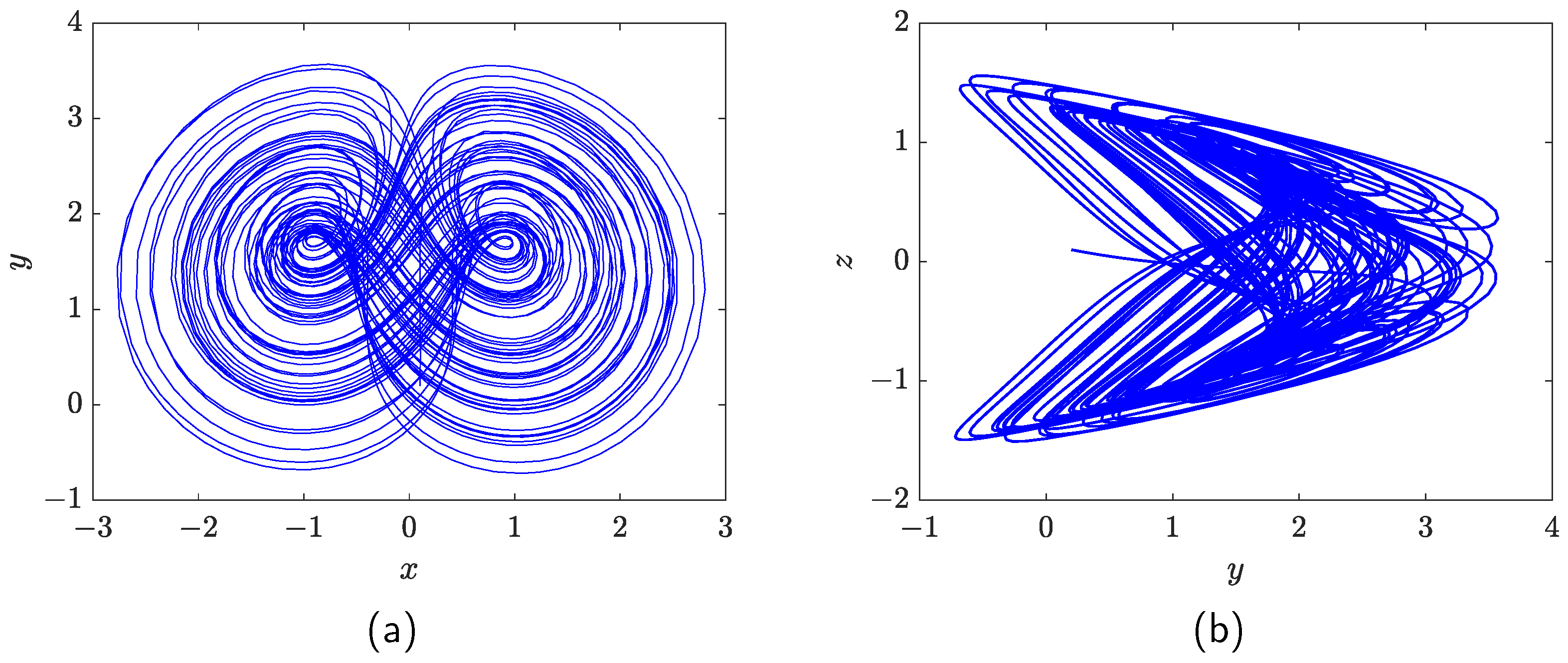
2. Dynamic Analysis of the Financial System

According to references [7,8,36], a 3D financial system is established based on four sub-blocks: labor force, stock, money, and production. And the mathematical expression of a financial system is given as follows:

$$\left\{\begin{array}{cc}\hfill \dot{x}& =z+(y-a)x,\hfill \\ \hfill \dot{y}& =1-by-x^2,\hfill \\ \hfill \dot{z}& =-x-cz,\hfill \end{array}\right.$$

(1)

where the variables $x,y,z$ represent the interest rate, investment demand, and price indices, respectively. And the parameters $a,b,c$ ($a,b,c⩾0$) are the saving, investment cost, and demand elasticity of the commodity, respectively. Hence, the Jacobian matrix of the system (1) is given by

$$J(x,y)=\left[\begin{array}{ccc}y-a& x& 1\\ 2x& -b& 0\\ -1& 0& -c\end{array}\right],$$

and the Lyapunov exponents of the system (1) can be obtained when $a=0.9$, $b=0.1$, and $c=1$ [7,8,36], i.e.,

$$\begin{array}{c}\hfill {\mathrm{LE}}_1=0.1401,{\mathrm{LE}}_2=0.0000,{\mathrm{LE}}_3=-0.5302.\end{array}$$

The Lyapunov exponent is used to characterize the degree of convergence and dispersion of trajectories in a dynamical system. According to chaos theory, if there is a positive Lyapunov exponent, a zero exponent, and a negative exponent in a dynamical system, then the system is in a chaotic state. Obviously, in the system (1) exists a positive Lyapunov exponent ${\mathrm{LE}}_1$, so it is in a chaotic state.

The chaotic attractors of the system (1) are shown in Figure 1 when the initial values are $\left(x\right(0),y(0),z(0\left)\right)=$$(0.1,0.2,0.1)$. Obviously, the variables $x, y$ and z are globally bounded and stable but locally unstable, and it has a high sensitivity to initial values.

2.1. Equilibrium Point of Financial System (1)

The equilibrium points of the financial system (1) are given by

$$\begin{array}{c}\hfill z+(y-a)x=0,1-by-x^2=0,-x-cz=0,\end{array}$$

so the equilibrium points are obtained by $(x^{\left(e\right)},y^{\left(e\right)},z^{\left(e\right)})=(0,1/b,0)$, and

$$\begin{array}{c}\hfill (x^{\left(e\right)},y^{\left(e\right)},z^{\left(e\right)})=\left(\pm \left(\right(ac+1)b/c-1),(ac+1)b/c,\pm [1-(ac+1)b/c]/c\right).\end{array}$$

(2)

Therefore, the Jacobian matrix at the equilibrium point $(0,1/b,0)$ is given by

$$J_1=\left[\begin{array}{ccc}1/b-a& 0& 1\\ 0& -b& 0\\ -1& 0& -c\end{array}\right],$$

so the corresponding eigenvalues are equal to ${\lambda }_1=9,{\lambda }_2=-0.9,{\lambda }_3=-0.1$. As there is a positive eigenvalue, the system (1) is unstable at this equilibrium point. Similarly, the Jacobian matrices $J_2$ and $J_3$ at the equilibrium points in Equation (2) are given by

$$J_{2,3}=\left[\begin{array}{ccc}(ac+1)b/c-a& \pm \left(\right(ac+1)b/c-1)& 1\\ \pm 2\left(\right(ac+1)b/c-1)& -b& 0\\ -1& 0& -c\end{array}\right],$$

and the eigenvalues of $J_2$ and $J_3$ are given by [37]

$$\begin{array}{cc}\hfill {\lambda }_1^{J_2}& =0.5820,{\lambda }_{2,3}^{J_2}=-1.1960\pm 0.7293\mathrm{i};{\lambda }_1^{J_3}=0.5820,{\lambda }_{2,3}^{J_3}=-1.1960\pm 0.7284\mathrm{i}.\hfill \end{array}$$

Obviously, the system (1) at these equilibrium points in Equation (2) is also unstable.

2.2. Bifurcation Analysis of Financial System (1)

There are three parameters $a,b$, and c in the financial system (1), and they exhibit chaotic behavior when $a=0.9$, $b=0.1$, and $c=1$. If one wants to control the system through its parameters, which parameter will be more effective? Therefore, a further discussion of this problem is given by the bifurcation with respect to the parameters, and the bifurcation of system (1) is shown in Figure 2a according to the bifurcation algorithm of a dynamical system in Algorithm 1. Meanwhile, the Lyapunov exponent spectrum is also shown in Figure 2b.

Algorithm 1: Algorithm of Bifurcation with Respect to Parameter c

Input: Parameters $a,b$, initial values $x\left(0\right),y\left(0\right),z\left(0\right)$, $c\in [c_l,c_r]$, step of parameter c: $h_c=0.01$; $t\in [0,T]$, step of time t: $h=0.001$, allowable error ${\delta }_0$ Output: Poincaré cross-section points P when $x=y$ 1 Calculate $N_c=\mathrm{round}((c_r-c_l)/h_c)$, $N=T/h$, $i=1,j=1$ 2 Generate variables $x,y$ and z based on system (1): 3 for $i⩽N$ do 4       $x\left(i\right)=x(i-1)+\dot{x}(i-1)h$ 5       $y\left(i\right)=y(i-1)+\dot{y}(i-1)h$ 6       $z\left(i\right)=z(i-1)+\dot{z}(i-1)h$ 7       $i=i+1$ 8 end 9 for $j⩽N_c$ do$\phantom{(}$ 10       if $|x\left(j\right)-y\left(j\right)|⩽{\delta }_0$ then 11           $P(j,:)=z\left(j\right)$ 12       end 13       $j=j+1$; 14 end

Based on the Lyapunov exponent spectrum and the bifurcation diagram with respect to parameter c, the system (1) exhibits chaotic behavior when $c\in (0.6,1.1)$, but it exhibits periodic behavior when $c\in (0.1,0.6)\cup (1.1,2)$. So, the dynamic behavior of the system (1) can be controlled by the demand elasticity of the commodity c. For example, the attractor of the financial system is shown in Figure 3 when $c=2$. Obviously, it can be in a periodic state when the parameter c changed from 1 to 2.

Remark 1.

Similarly, the bifurcation algorithm can also be used to calculate the bifurcation diagrams with respect to parameters a and b. According to the results of bifurcation, the system (1) keeps at a state of chaos when the parameters a and b belong to the interval $[0,3]$. Therefore, if one wants to control the behavior of the financial system (1) to be periodic, then the parameter c may be better than parameters a and b.

3. Consensus Control of Master–Slave Systems

3.1. Consensus Control of Master–Slave Financial Systems

The master system is given by financial system (1), and the slave system with linear controllers $u_x,u_y$ can be obtained as follows:

$$\left\{\begin{array}{cc}\hfill {\dot{x}}_1& =z_1+(y_1-a)x_1+u_x,\hfill \\ \hfill {\dot{y}}_1& =1-b{y}_1-x_1^2+u_y,\hfill \\ \hfill {\dot{z}}_1& =-x_1-c{z}_1,\hfill \end{array}\right.$$

(3)

where $a=0.9,b=0.1,c=1$, $u_x$, and $u_y$ are linear controllers. If one defines the errors $e_x=x-x_1,e_y=y-y_1,e_z=z-z_1$, then the error system is obtained by

$$\left\{\begin{array}{cc}\hfill {\dot{e}}_x& =e_z-a{e}_x+y{e}_x+x_1{e}_y-u_x,\hfill \\ \hfill {\dot{e}}_y& =-b{e}_y-(x+x_1)e_x-u_y,\hfill \\ \hfill {\dot{e}}_z& =-e_x-c{e}_z,\hfill \end{array}\right.$$

(4)

where $u_x=k_x{e}_x,u_y=k_y{e}_y$.

Definition 1.

If the errors $e_x,e_y$, and $e_z$ of Equation (4) tend to zero as time $t\to +\infty$, then the master–slave systems (1) and (3) have achieved synchronization or consensus.

Theorem 1.

If the suitable gain coefficients $k_x$ and $k_y$ are chosen such that

$$\begin{array}{cc}\hfill k_x& >-a+y+1,k_y>-b+x^2/4,\hfill \end{array}$$

(5)

then the master–slave systems (1) and (3) are globally synchronized.

Proof of Theorem 1.

According to the error system (4), if the Lyapunov function is

$$\begin{array}{c}\hfill V=(e_x^2+e_y^2+e_z^2)/2,\end{array}$$

then its derivative is

$$\begin{array}{cc}\hfill \dot{V}& =e_x{\dot{e}}_x+e_y{\dot{e}}_y+e_z{\dot{e}}_z\hfill \\ & =e_x(e_z-a{e}_x+y{e}_x+x_1{e}_y-u_x)+e_y(-b{e}_y-(x+x_1)e_x-u_y)+e_z(-e_x-c{e}_z)\hfill \\ & =(-a+y-k_x)e_x^2+(-b-k_y)e_y^2-c{e}_z^2-x{e}_x{e}_y\hfill \\ & =(-a+y+1-k_x)e_x^2+(-b+x^2/4-k_y)e_y^2-c{e}_z^2-{(e_x+x{e}_y/2)}^2.\hfill \end{array}$$

According the condition in Equation (5), one has $\dot{V}<0$. According to the Lyapunov stability theory [38,39], the system (4) is globally exponentially stable about the origin if $k_x>-a+y+1$, $k_y>-b+x^2/4$, i.e., the master–slave systems (1) and (3) are globally synchronized. □

Example 1.

According to the attractor of system (1), the variables $x,y$ satisfy $\left|x\right|<3,y<4$, so the gain coefficients of the controllers $u_x$ and $u_y$ can be given by $k_x=4.1,k_y=2.2$ based on Theorem 1. And the initial values of master–slave systems are $\left(x\right(0),y(0),z(0\left)\right)=(0.1,0.2,0.1)$, and $(x_1\left(0\right),$$y_1\left(0\right),$$z_1\left(0\right))$$=(0.2,0.1,0.3)$, respectively.

The synchronization errors $e_x,e_y$, and $e_z$ are shown in Figure 4 by Matlab R2020b. Obviously, the master–slave systems have reached consensus as $t\to +\infty$.

Remark 2.

Consensus control usually refers to the consensus problem among multiple systems. In this paper, only the synchronization control method for master–slave systems is proposed, because the topological network structure between multiple systems is not provided. However, this control method can be extended to multiple slave systems to synchronize with the master system (1), and then the consensus control among multiple systems is easily obtained. Furthermore, the new slave systems can also be designed to synchronize with the slave system (3), so the consensus control for multiple systems is also achieved in the end.

3.2. Consensus of Master–Slave Systems with Unknown Parameters

If the parameters $a,b,c$ of master system (1) are unknown, then the slave system with estimated parameters $\widehat{a},\widehat{b},\widehat{c}$ and linear controllers can be given as follows:

$$\left\{\begin{array}{cc}\hfill {\dot{x}}_1& =z_1+(y_1-\widehat{a})x_1+u_x,\hfill \\ \hfill {\dot{y}}_1& =1-\widehat{b}{y}_1-x_1^2+u_y,\hfill \\ \hfill {\dot{z}}_1& =-x_1-\widehat{c}{z}_1\hfill \end{array}\right.$$

(6)

where $\widehat{a},\widehat{b},\widehat{c}$ are the estimations of parameters $a,b,c$, respectively. And $u_x,u_y$ are linear controllers. If the errors are $e_x=x-x_1$,$e_y=y-y_1$,$e_z=z-z_1$, $e_a=a-\widehat{a}$, $e_b=b-\widehat{b}$, and $e_c=c-\widehat{c}$, then the error system is obtained by

$$\left\{\begin{array}{cc}\hfill {\dot{e}}_x& =e_z-a{e}_x-x_1{e}_a+y{e}_x+x_1{e}_y-u_x,\hfill \\ \hfill {\dot{e}}_y& =-b{e}_y-y_1{e}_b-(x+x_1)e_x-u_y,\hfill \\ \hfill {\dot{e}}_z& =-e_x-c{e}_z-z_1{e}_c,\hfill \end{array}\right.$$

(7)

where $u_x=k_x{e}_x,u_y=k_y{e}_y$.

Theorem 2.

If the suitable gain coefficients $k_x$ and $k_y$ are chosen such that

$$\begin{array}{cc}\hfill k_x& >-a+y+1,k_y>-b+x^2/4,\hfill \end{array}$$

(8)

and the adaptive laws for estimated parameters $\widehat{a},\widehat{b},\widehat{c}$ are given by

$$\begin{array}{c}\hfill \dot{\widehat{a}}=-x_1(x-x_1),\dot{\widehat{b}}=-y_1(y-y_1),\dot{\widehat{c}}=-z_1(z-z_1),\end{array}$$

(9)

then the master–slave systems (1) and (6) are globally synchronized.

Proof Theorem 2.

According to the system (7), if the Lyapunov function is given by

$$\begin{array}{c}\hfill V=(e_x^2+e_y^2+e_z^2+e_a^2+e_b^2+e_c^2)/2\end{array}$$

then its derivative is

$$\begin{array}{cc}\hfill \dot{V}& =e_x{\dot{e}}_x+e_y{\dot{e}}_y+e_z{\dot{e}}_z+e_a{\dot{e}}_a+e_b{\dot{e}}_b+e_c{\dot{e}}_c\hfill \\ & =e_x(e_z-a{e}_x-x_1{e}_a+y{e}_x+x_1{e}_y-u_x)+e_y(-b{e}_y-y_1{e}_b-(x+x_1)e_x-u_y)\hfill \\ & +e_z(-e_x-c{e}_z-z_1{e}_c)+e_a{\dot{e}}_a+e_b{\dot{e}}_b+e_c{\dot{e}}_c\hfill \\ & =e_x^2(1-a+y-k_x)+e_y^2(-b+x^2/4-k_y)-c{e}_z^2-x_1{e}_x{e}_a+e_a{\dot{e}}_a-y_1{e}_y{e}_b+e_b{\dot{e}}_b\hfill \\ & -z_1{e}_z{e}_c+e_c{\dot{e}}_c.\hfill \end{array}$$

If the following conditions are satisfied, i.e., $-x_1{e}_x{e}_a+e_a{\dot{e}}_a=0$, $-y_1{e}_y{e}_b+e_b{\dot{e}}_b=0$, $-z_1{e}_z{e}_c$$+e_c{\dot{e}}_c=0,$ then one has $e_a=0,e_b=0,e_c=0$, or $\dot{\widehat{a}}=-x_1(x-x_1)$, $\dot{\widehat{b}}=-y_1(y-y_1)$, $\dot{\widehat{c}}=-z_1(z-z_1).$

Therefore, one has $\dot{V}<0$ by the condition in Equation (8). According to the Lyapunov stability theory, the system (7) is globally exponentially stable about the origin if $k_x>-a+y+1,k_y>-b+x^2/4$, i.e., the master–slave systems (1) and (6) are globally synchronized. □

Example 2.

The gain coefficients $k_x=4.1,k_y=2.2$ according to Theorem 2, and the initial values of master–slave systems are given by $\left(x\right(0),y(0),z(0\left)\right)$$=(0.1,0.2,0.1)$, $(x_1\left(0\right),$$y_1\left(0\right),$$z_1\left(0\right))$$=(0.2,0.1,0.3)$, and $(\widehat{a}\left(0\right),\widehat{b}\left(0\right),\widehat{c}\left(0\right))$$=(0.8,$$0.2,$$0.7)$, respectively.

The synchronization errors $e_x,e_y$, and $e_z$ are shown in Figure 5a. The master–slave systems have reached consensus as $t\to +\infty$. In Figure 5b, the parameters $\widehat{a},\widehat{b},\widehat{c}$ of slave system (6) can track to the $a,b,c$ of master system (1) as $t\to +\infty$.

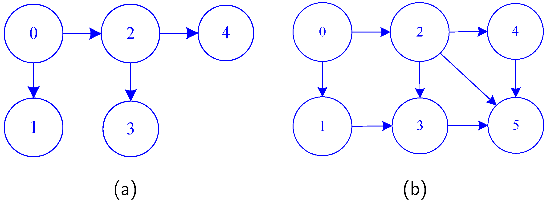
4. Consensus of Leader–Follower Multi-Agent Systems with Unknown Parameters

In this section, the consensus of leader–follower multi-agent systems with unknown parameters is discussed in terms of the Lyapunov stability theorem. The definition of the consensus of leader–follower multi-agent systems is given as follows.

Definition 2.

The leader–follower multi-agent systems are consistent if the following conditions are satisfied: $\underset{t\to +\infty }{lim}{e}_{0i}=0,i=1,2,\cdots$, where $e_{0i}$ denotes the error between the leader and ith follower.

4.1. Consensus of Leader–Follower Multi-Agent Systems

As the financial system (1) behaves with a complex motion trajectory when it is at a state of chaos, so it is chosen as the leader system, i.e.,

$$\left\{\begin{array}{cc}\hfill {\dot{x}}_0& =z_0+(y_0-a)x_0,\hfill \\ \hfill {\dot{y}}_0& =1-b{y}_0-x_0^2,\hfill \\ \hfill {\dot{z}}_0& =-x_0-c{z}_0.\hfill \end{array}\right.$$

(10)

The ith ($i=1,2,\cdots$) follower system with estimated parameters ${\widehat{a}}_i,{\widehat{b}}_i,{\widehat{c}}_i$ and two linear controllers $u_{0i}^{\left(x\right)},u_{0i}^{\left(y\right)}$ is given as follows:

$$\left\{\begin{array}{cc}\hfill {\dot{x}}_i& =z_i+(y_i-{\widehat{a}}_i)x_i+u_{0i}^{\left(x\right)},\hfill \\ \hfill {\dot{y}}_i& =1-{\widehat{b}}_i{y}_i-x_i^2+u_{0i}^{\left(y\right)},\hfill \\ \hfill {\dot{z}}_i& =-x_i-{\widehat{c}}_i{z}_i,\hfill \end{array}\right.$$

(11)

where ${\widehat{a}}_i,{\widehat{b}}_i,{\widehat{c}}_i$ are the estimations of parameters $a,b,c$, respectively. And $u_{0i}^{\left(x\right)},u_{0i}^{\left(y\right)}$ are the linear feedback controllers of ith follower. If the errors of the leader and ith follower are given by

$$\begin{array}{c}\hfill e_{0i}^{\left(x\right)}=x_0-x_i,e_{0i}^{\left(y\right)}=y_0-y_i,e_{0i}^{\left(z\right)}=z_0-z_i,e_{0i}^{\left(a\right)}=a-{\widehat{a}}_i,e_{0i}^{\left(b\right)}=b-{\widehat{b}}_i,e_{0i}^{\left(c\right)}=c-{\widehat{c}}_i,\end{array}$$

then the error system between the leader and ith follower is obtained by

$$\left\{\begin{array}{cc}\hfill {\dot{e}}_{0i}^{\left(x\right)}& =e_{0i}^{\left(z\right)}-a{e}_{0i}^{\left(x\right)}-x_i{e}_{0i}^{\left(a\right)}+y_0{e}_{0i}^{\left(x\right)}+x_i{e}_{0i}^{\left(y\right)}-u_{0i}^{\left(x\right)},\hfill \\ \hfill {\dot{e}}_{0i}^{\left(y\right)}& =-b{e}_{0i}^{\left(y\right)}-y_i{e}_{0i}^{\left(b\right)}-(x_0+x_i)e_{0i}^{\left(x\right)}-u_{0i}^{\left(y\right)},\hfill \\ \hfill {\dot{e}}_{0i}^{\left(z\right)}& =-e_{0i}^{\left(x\right)}-c{e}_{0i}^{\left(z\right)}-z_i{e}_{0i}^{\left(c\right)},\hfill \end{array}\right.$$

(12)

where $u_{0i}^{\left(x\right)}=a_{0i}{k}_{0i}^{\left(x\right)}{e}_{0i}^{\left(x\right)}+{\displaystyle \sum _{j=1}^N}{a}_{ij}{k}_{ij}^{\left(x\right)}(x_i-x_j)$, $u_{0i}^{\left(y\right)}=a_{0i}{k}_{0i}^{\left(y\right)}{e}_{0i}^{\left(y\right)}+{\displaystyle \sum _{j=1}^N}{a}_{ij}{k}_{ij}^{\left(y\right)}(y_i-y_j)$, $(i=1,2,\cdots )$.

The $a_{ij}$ denotes the connection between ith and jth agents. If there is an edge between followers i and j, then $a_{ij}=1$. And $a_{ij}=0$ if there is not any edge between the ith and jth followers. $k_{ij}^{\left(x\right)}$ and $k_{ij}^{\left(y\right)}$ are the feedback gains, and the $k_{ij}^{\left(x\right)}=k_{ij}^{\left(y\right)}=0$ in the case of $a_{0i}=1$. Obviously, it is easy to obtain the following Theorem 3 based on Theorem 2.

Theorem 3.

If the suitable gain coefficients $k_{0i}^{\left(x\right)}$ and $k_{0i}^{\left(y\right)}$$(i=0,1,\cdots )$ are chosen such that

$$\begin{array}{cc}\hfill k_{0i}^{\left(x\right)}& >-a+y_0+1,k_{0i}^{\left(y\right)}>-b+x_0^2/4,\hfill \end{array}$$

(13)

and the adaptive laws for estimated parameters ${\widehat{a}}_i,{\widehat{b}}_i,{\widehat{c}}_i$ are given by

$$\begin{array}{c}\hfill {\dot{\widehat{a}}}_i=-a_{0i}{x}_i(x_0-x_i),{\dot{\widehat{b}}}_i=-a_{0i}{y}_i(y_0-y_i),{\dot{\widehat{c}}}_i=-a_{0i}{z}_i(z_0-z_i),\end{array}$$

(14)

then the leader–follower systems (10) and (11) are globally synchronized.

Similarly, the jth ($j=2,\cdots$) follower system with estimated parameters ${\widehat{a}}_j,{\widehat{b}}_j,{\widehat{c}}_j$ and linear feedback controllers $u_{ij}^{\left(x\right)},u_{ij}^{\left(y\right)}$ is given as follows:

$$\left\{\begin{array}{cc}\hfill {\dot{x}}_j& =z_j+(y_j-{\widehat{a}}_j)x_j+u_{ij}^{\left(x\right)}\hfill \\ \hfill {\dot{y}}_j& =1-{\widehat{b}}_j{y}_j-x_j^2+u_{ij}^{\left(y\right)}\hfill \\ \hfill {\dot{z}}_j& =-x_j-{\widehat{c}}_j{z}_j\hfill \end{array}\right.$$

(15)

If the jth follower is connected with the ith follower, and the errors between the ith and jth followers are defined as

$$\begin{array}{c}\hfill e_{ij}^{\left(x\right)}=x_i-x_j,e_{ij}^{\left(y\right)}=y_i-y_j,e_{ij}^{\left(z\right)}=z_i-z_j,e_{ij}^{\left(a\right)}=a_i-{\widehat{a}}_j,e_{ij}^{\left(b\right)}=b_i-{\widehat{b}}_j,e_{ij}^{\left(c\right)}=c_i-{\widehat{c}}_j,\end{array}$$

then the error system between the ith and jth followers is obtained as follows

$$\left\{\begin{array}{cc}\hfill {\dot{e}}_{ij}^{\left(x\right)}& =e_{ij}^{\left(z\right)}-{\widehat{a}}_i{e}_{ij}^{\left(x\right)}-x_j{e}_{ij}^{\left(a\right)}+y_i{e}_{ij}^{\left(x\right)}+x_j{e}_{ij}^{\left(y\right)}+u_{0i}^{\left(x\right)}-u_{ij}^{\left(x\right)},\hfill \\ \hfill {\dot{e}}_{ij}^{\left(y\right)}& =-{\widehat{b}}_i{e}_{ij}^{\left(y\right)}-y_j{e}_{ij}^{\left(b\right)}-(x_i+x_j)e_{ij}^{\left(x\right)}+u_{0i}^{\left(y\right)}-u_{ij}^{\left(y\right)},\hfill \\ \hfill {\dot{e}}_{ij}^{\left(z\right)}& =-e_{ij}^{\left(x\right)}-{\widehat{c}}_i{e}_{ij}^{\left(z\right)}-z_j{e}_{ij}^{\left(c\right)},\hfill \end{array}\right.$$

(16)

where $u_{ij}^{\left(x\right)}={\displaystyle \sum _{j=1}^N}{a}_{ij}{k}_{ij}^{\left(x\right)}(x_i-x_j),u_{ij}^{\left(y\right)}={\displaystyle \sum _{j=1}^N}{a}_{ij}{k}_{ij}^{\left(y\right)}(y_i-y_j)$ ($i=1,2,\cdots$).

Theorem 4.

If the suitable gain coefficients $k_{ij}^{\left(x\right)}$ and $k_{ij}^{\left(y\right)}$$(i,j=0,1,\cdots )$ are chosen such that

$$\begin{array}{cc}\hfill k_{ij}^{\left(x\right)}& >1-{\widehat{a}}_i+y_i,k_{ij}^{\left(y\right)}>-\widehat{b}+x_i^2/4,\hfill \end{array}$$

(17)

and the adaptive laws for estimated parameters ${\widehat{a}}_j,{\widehat{b}}_j,{\widehat{c}}_j$ are given by

$$\begin{array}{c}\hfill {\dot{\widehat{a}}}_j=-x_j{e}_{ij}^{\left(x\right)},{\dot{\widehat{b}}}_j=-y_j{e}_{ij}^{\left(y\right)},{\dot{\widehat{c}}}_j=-z_j{e}_{ij}^{\left(z\right)},\end{array}$$

(18)

then the ith follower in system (11) and jth follower in Equation (15) are globally synchronized.

Proof of Theorem 4.

According to the error system (16), the synchronization of ith follower and jth follower is proved by the Lyapunov stability theorem, and the Lyapunov function of the ith follower and the jth follower is given by

$$\begin{array}{c}\hfill V_{ij}=({\left(e_{ij}^{\left(x\right)}\right)}^2+{\left(e_{ij}^{\left(y\right)}\right)}^2+{\left(e_{ij}^{\left(z\right)}\right)}^2+{\left(e_{ij}^{\left(a\right)}\right)}^2+{\left(e_{ij}^{\left(b\right)}\right)}^2+{\left(e_{ij}^{\left(c\right)}\right)}^2)/2,\end{array}$$

and the $a_{0i}=0,k_{ij}^{\left(x\right)},k_{ij}^{\left(y\right)}>0$; then, its derivative is

$$\begin{array}{cc}\hfill {\dot{V}}_{ij}& =e_{ij}^{\left(x\right)}{\dot{e}}_{ij}^{\left(x\right)}+e_{ij}^{\left(y\right)}{\dot{e}}_{ij}^{\left(y\right)}+e_{ij}^{\left(z\right)}{\dot{e}}_{ij}^{\left(z\right)}+e_{ij}^{\left(a\right)}{\dot{e}}_{ij}^{\left(a\right)}+e_{ij}^{\left(b\right)}{\dot{e}}_{ij}^{\left(b\right)}+e_{ij}^{\left(c\right)}{\dot{e}}_{ij}^{\left(c\right)}\hfill \\ & =e_{ij}^{\left(x\right)}(e_{ij}^{\left(z\right)}-{\widehat{a}}_i{e}_{ij}^{\left(x\right)}-x_j{e}_{ij}^{\left(a\right)}+y_i{e}_{ij}^{\left(x\right)}+x_j{e}_{ij}^{\left(y\right)}-u_{ij}^{\left(x\right)})\hfill \\ & +e_{ij}^{\left(y\right)}(-{\widehat{b}}_i{e}_{ij}^{\left(y\right)}-y_j{e}_{ij}^{\left(b\right)}-(x_i+x_j)e_{ij}^{\left(x\right)}-u_{ij}^{\left(y\right)})\hfill \\ & +e_{ij}^{\left(z\right)}(-e_{ij}^{\left(x\right)}-{\widehat{c}}_i{e}_{ij}^{\left(z\right)}-z_j{e}_{ij}^{\left(c\right)})+e_{ij}^{\left(a\right)}{\dot{e}}_{ij}^{\left(a\right)}+e_{ij}^{\left(b\right)}{\dot{e}}_{ij}^{\left(b\right)}+e_{ij}^{\left(c\right)}{\dot{e}}_{ij}^{\left(c\right)}\hfill \\ & ={\left(e_{ij}^{\left(x\right)}\right)}^2(1-{\widehat{a}}_i+y_i-k_{ij}^{\left(x\right)}{a}_{ij})+{\left(e_{ij}^{\left(y\right)}\right)}^2(-{\widehat{b}}_i+x_i^2/4-a_{ij}{k}_{ij}^{\left(y\right)})-{\widehat{c}}_i{\left(e_{ij}^{\left(z\right)}\right)}^2\hfill \\ & -e_{ij}^{\left(x\right)}\sum _{l=1,l\ne j}^N{a}_{il}{k}_{il}^{\left(x\right)}(x_i-x_l)-e_{ij}^{\left(y\right)}\sum _{l=1,l\ne j}^N{a}_{il}{k}_{il}^{\left(y\right)}(y_i-y_l)\hfill \\ & -x_j{e}_{ij}^{\left(x\right)}{e}_{ij}^{\left(a\right)}+e_{ij}^{\left(a\right)}{\dot{e}}_{ij}^{\left(a\right)}-y_j{e}_{ij}^{\left(y\right)}{e}_{ij}^{\left(b\right)}+e_{ij}^{\left(b\right)}{\dot{e}}_{ij}^{\left(b\right)}-z_j{e}_{ij}^{\left(z\right)}{e}_{ij}^{\left(c\right)}+e_{ij}^{\left(c\right)}{\dot{e}}_{ij}^{\left(c\right)}.\hfill \end{array}$$

If the following conditions are satisfied, i.e.,

$$\begin{array}{c}\hfill -x_j{e}_{ij}^{\left(x\right)}{e}_{ij}^{\left(a\right)}+e_{ij}^{\left(a\right)}{\dot{e}}_{ij}^{\left(a\right)}=0,-y_j{e}_{ij}^{\left(y\right)}{e}_{ij}^{\left(b\right)}+e_{ij}^{\left(b\right)}{\dot{e}}_{ij}^{\left(b\right)}=0,-z_j{e}_{ij}^{\left(z\right)}{e}_{ij}^{\left(c\right)}+e_{ij}^{\left(c\right)}{\dot{e}}_{ij}^{\left(c\right)}=0,\end{array}$$

then one has $e_{ij}^{\left(a\right)}=0,e_{ij}^{\left(b\right)}=0,e_{ij}^{\left(c\right)}=0$, or ${\dot{\widehat{a}}}_j=-x_j{e}_{ij}^{\left(x\right)},{\dot{\widehat{b}}}_j=-y_j{e}_{ij}^{\left(y\right)},{\dot{\widehat{c}}}_j=-z_j{e}_{ij}^{\left(z\right)}$.

The ith follower is synchronized with the leader as $t\to +\infty$, so the ith follower will synchronize with the lth follower as $t\to +\infty$, i.e.,

$$\left\{\begin{array}{cc}& \underset{t\to +\infty }{lim}(x_i-x_l)=0,\underset{t\to +\infty }{lim}(y_i-y_l)=0,\underset{t\to +\infty }{lim}(z_i-z_l)=0,\hfill \\ & \underset{t\to +\infty }{lim}({\widehat{a}}_i-a_l)=0,\underset{t\to +\infty }{lim}({\widehat{b}}_i-b_l)=0,\underset{t\to +\infty }{lim}({\widehat{c}}_i-c_l)=0.\hfill \end{array}\right.(l\ne j)$$

As the $a_{il}$, $k_{il}^{\left(x\right)},k_{il}^{\left(y\right)},k_{il}^{\left(z\right)}$ are bounded, one has

$$\begin{array}{cc}& \underset{t\to +\infty }{lim}\sum _{l=1,l\ne j}^N{a}_{il}{k}_{il}^{\left(x\right)}(x_i-x_l)=0,\underset{t\to +\infty }{lim}\sum _{l=1,l\ne j}^N{a}_{il}{k}_{il}^{\left(y\right)}(y_i-y_l)=0.\hfill \end{array}$$

Therefore, one has ${\dot{V}}_{ij}<0$ by the condition in Equation (17). According to the Lyapunov stability theory, the error system (16) is globally exponentially stable about the origin if ${k_{ij}}^{\left(x\right)}>1-{\widehat{a}}_i+y_i,k_{ij}^{\left(y\right)}>-{\widehat{b}}_i+x_i^2/4$, i.e., the ith follower and jth follower in Equation (11) are globally synchronized. □

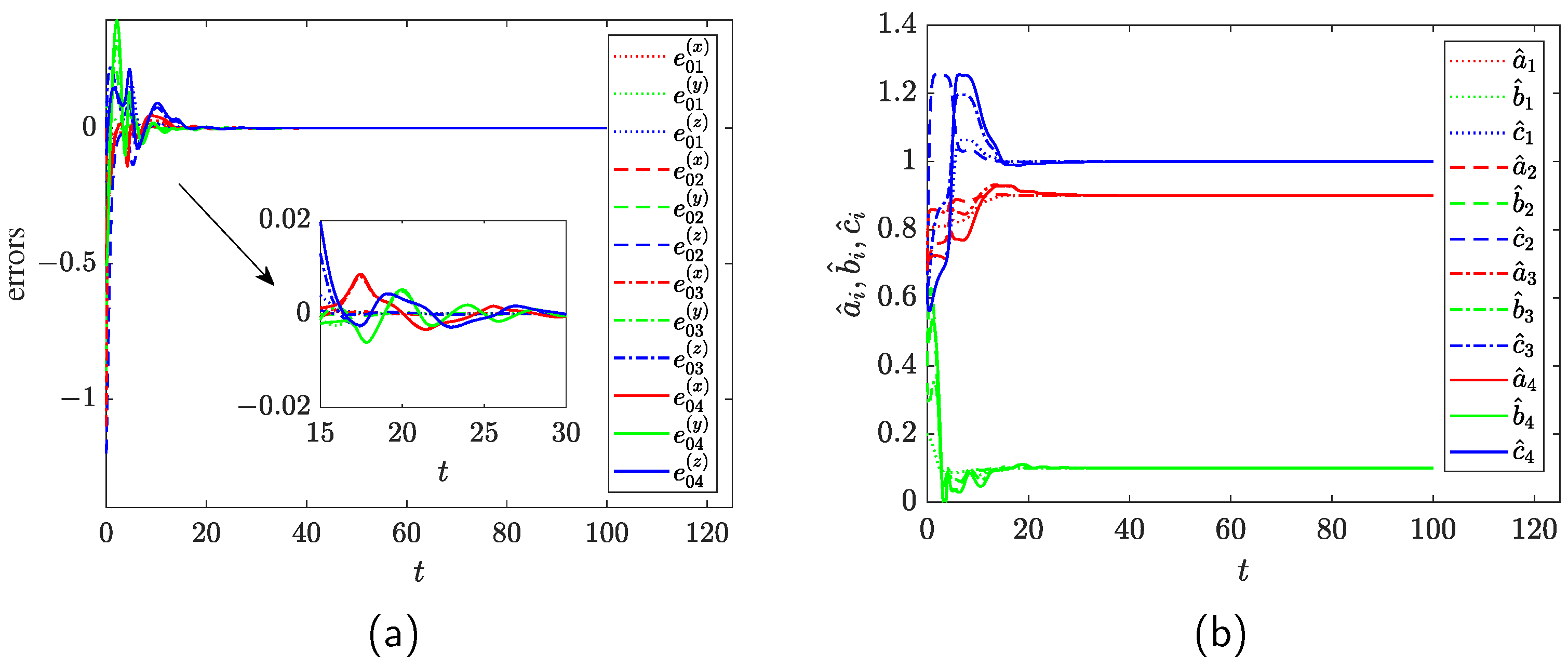
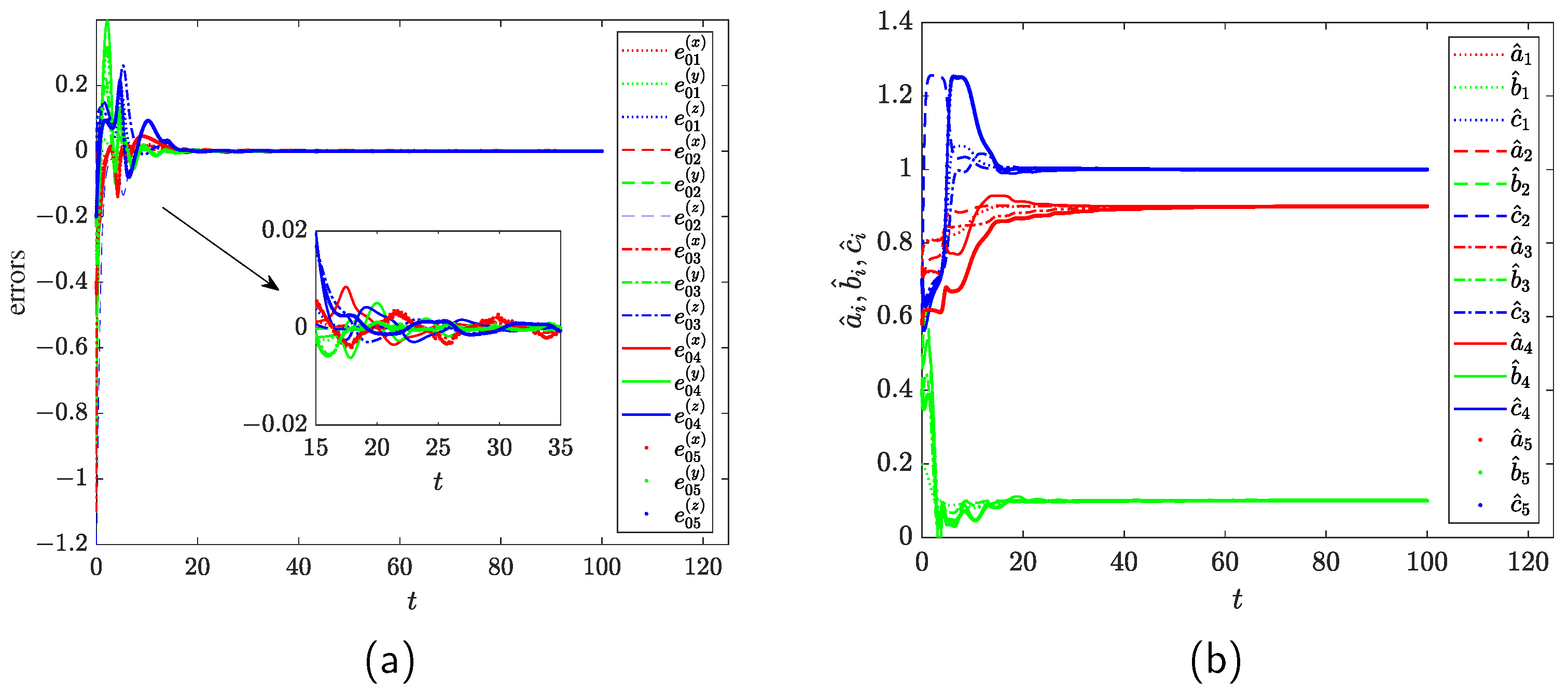
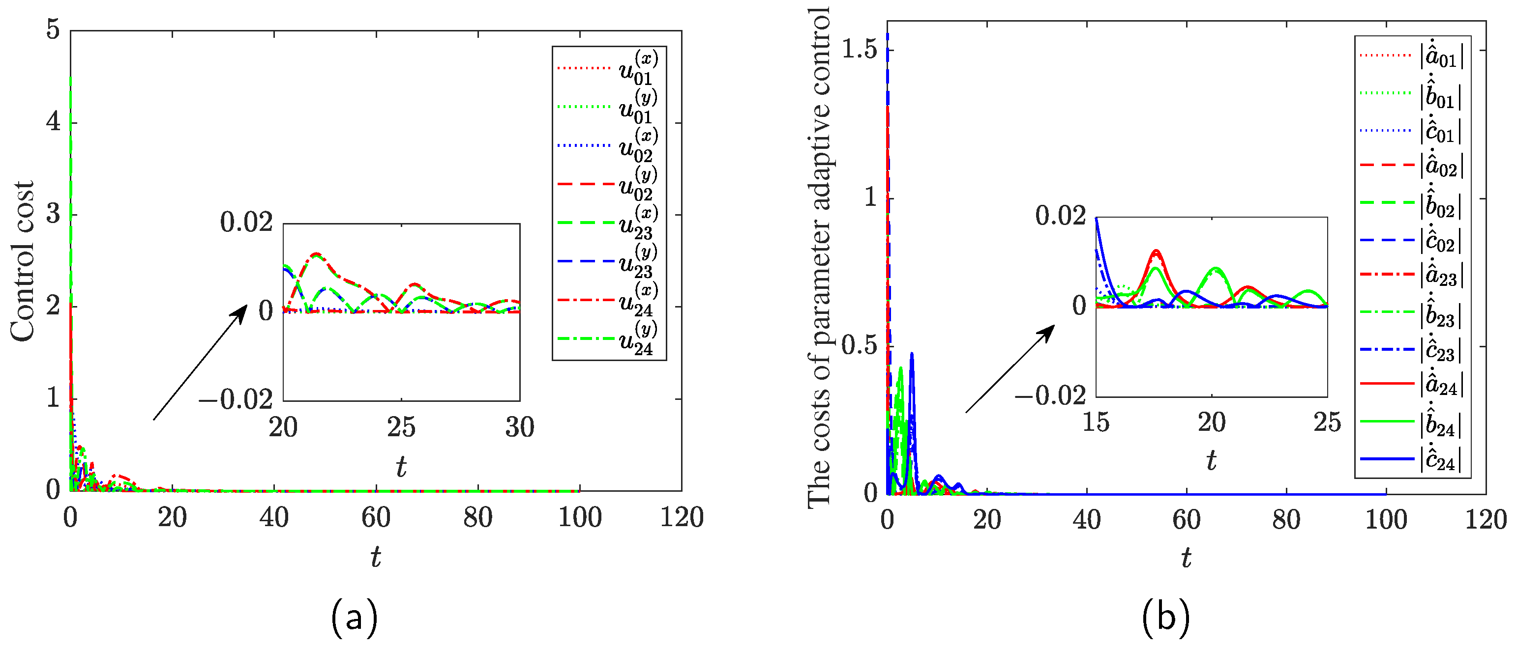
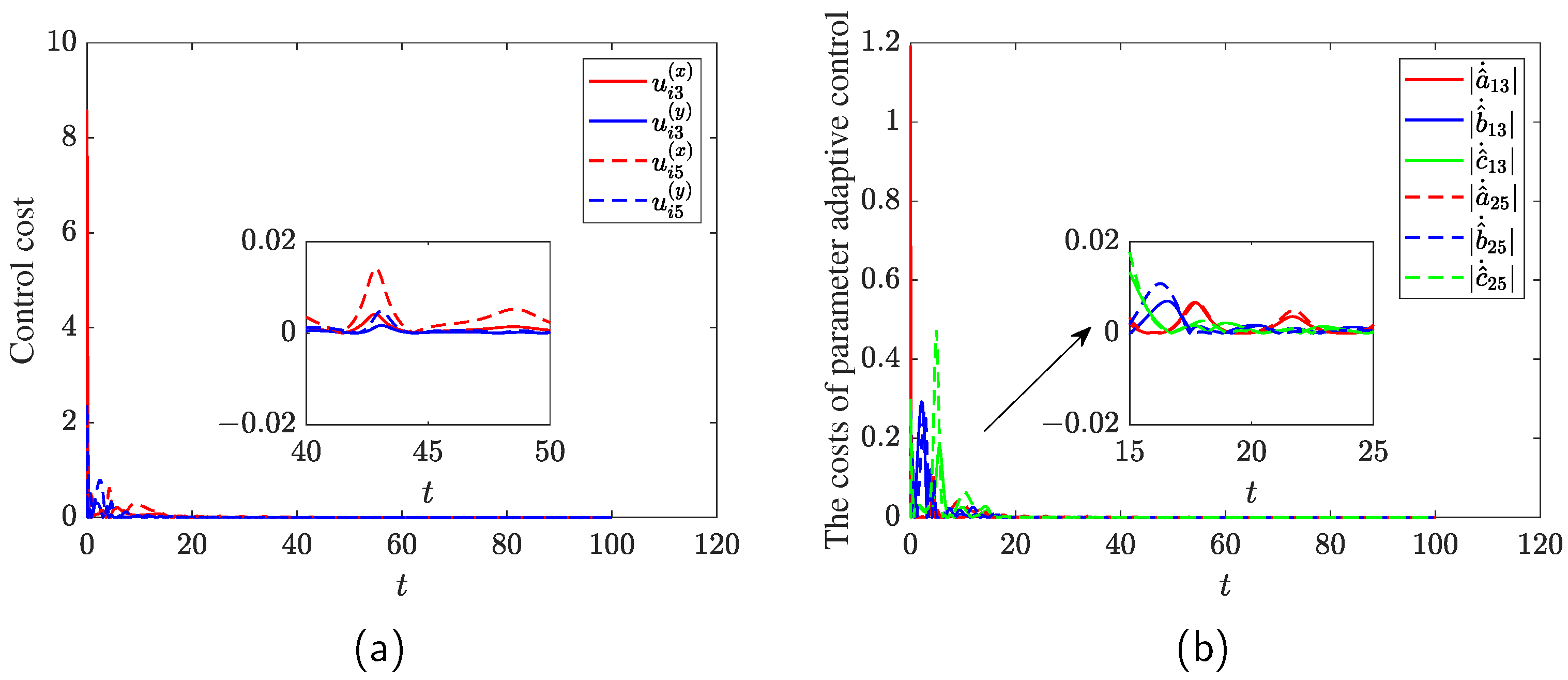
4.2. Numerical Simulations

Therefore, two examples of leader–follower multi-agent systems are given to show the proposed control method, and they are given as follows:

Example 3.

The leader–follower network among five agents is given in Figure 6a, where “0” denotes the leader, “1,2,3,4” denote the followers, the 1th and 2th followers are connected with leader, and the 3th and 4th followers are only connected with 2th follower.

The initial values $(x_i\left(0\right),y_i\left(0\right),z_i\left(0\right))$ and the parameters $({\widehat{a}}_i\left(0\right),{\widehat{b}}_i\left(0\right),{\widehat{c}}_i\left(0\right))$ of leader and followers are given by

$$\left\{\begin{array}{cc}\hfill (x_0\left(0\right),y_0\left(0\right),z_0\left(0\right))& =(0.1,0.2,0.1),(x_1\left(0\right),y_1\left(0\right),z_1\left(0\right))=(0.2,0.1,0.3),\hfill \\ \hfill (x_2\left(0\right),y_2\left(0\right),z_2\left(0\right))& =(0.1,1.1,1.3),(x_3\left(0\right),y_3\left(0\right),z_3\left(0\right))=(1.2,0.5,0.1),\hfill \\ \hfill (x_4\left(0\right),y_4\left(0\right),z_4\left(0\right))& =(0.6,0.7,0.2),k_{ij}^{\left(x\right)}=4.1,k_{ij}^{\left(y\right)}=2.2,\hfill \\ \hfill (a_0\left(0\right),b_0\left(0\right),c_0\left(0\right))& =(0.9,0.1,1),({\widehat{a}}_1\left(0\right),{\widehat{b}}_1\left(0\right),{\widehat{c}}_1\left(0\right))=(0.8,0.2,0.7),\hfill \\ \hfill ({\widehat{a}}_2\left(0\right),{\widehat{b}}_2\left(0\right),{\widehat{c}}_2\left(0\right))& =(0.7,0.4,0.6),({\widehat{a}}_3\left(0\right),{\widehat{b}}_3\left(0\right),{\widehat{c}}_3\left(0\right))=(0.71,0.35,0.64),\hfill \\ \hfill ({\widehat{a}}_4\left(0\right),{\widehat{b}}_4\left(0\right),{\widehat{c}}_4\left(0\right))& =(0.68,0.5,0.6).\hfill \end{array}\right.$$

(19)

The numerical simulation results based on Matlab R2020a are shown in Figure 7. All agents have reached consensus, and followers have also achieved accurate identification of the parameters of the leader system.

Example 4.

The leader–follower network among six agents is given in Figure 6b, where “0” denotes the leader and “1,2,3,4,5” denote the followers. Two followers are connected with leader, the 3th follower is connected with 1th and 2th follows, and 5th follower is connected with 4th, 3th, and 2th followers.

Similarly, the initial values $(x_i\left(0\right),y_i\left(0\right),z_i\left(0\right))$ of leader and followers are given in Equation (19), and the initials of the 5th follower are given by $(x_5\left(0\right),y_5\left(0\right),z_5\left(0\right))=(0.5,0.4,0.3)$; the initial estimated parameters are given by $({\widehat{a}}_5\left(0\right),{\widehat{b}}_5\left(0\right),{\widehat{c}}_5\left(0\right))=(0.58,0.4,0.7)$. The numerical simulation results based on Matlab R2020a are shown in Figure 8. All agents have reached consensus, and the followers have also achieved accurate identification of the parameters $a,b$, and c of the leader system.

Remark 3.

In the network of the agents in Figure 6b, the 3th agent communicates with 1th and 2th agents. Therefore, the parameters identification can choose the parameters of 1th or 2th agents to track and identify. Similarly, the 5th agent communicates with the 2th, 3th, and 4th agents, and then one of these agents can be selected for the parameters tracking and identification.

Remark 4.

Although there are only two simple leader–follower multi-agent systems are provided to verify the feasibility of linear feedback and adaptive method, the proposed method can be also extended to other complex leader–follower multi-agent systems, and the multi-agent systems can complete consensus as $t\to +\infty$.

4.3. Discussions of the Consensus for Multi-Agent Systems

In order to demonstrate the advantages of the proposed control method, the analysis of control costs and parameters adaptive laws are discussed with the initial errors:

$$\left\{\begin{array}{cc}\hfill |e_{01}^{\left(x\right)}\left(0\right)|& =0.1,|e_{01}^{\left(y\right)}\left(0\right)|=0.1,|e_{01}^{\left(z\right)}\left(0\right)|=0.2;\hfill \\ \hfill |e_{02}^{\left(x\right)}\left(0\right)|& =0.0,|e_{02}^{\left(y\right)}\left(0\right)|=0.9,|e_{02}^{\left(z\right)}\left(0\right)|=1.2;\hfill \\ \hfill |e_{23}^{\left(x\right)}\left(0\right)|& =1.1,|e_{23}^{\left(y\right)}\left(0\right)|=0.6,|e_{23}^{\left(z\right)}\left(0\right)|=1.2;\hfill \\ \hfill |e_{24}^{\left(x\right)}\left(0\right)|& =0.5,|e_{24}^{\left(y\right)}\left(0\right)|=0.4,|e_{24}^{\left(z\right)}\left(0\right)|=1.1,\hfill \end{array}\right.$$

(20)

and the initial parameters errors

$$\left\{\begin{array}{cc}\hfill |e_{01}^{\left(a\right)}\left(0\right)|& =0.1,|e_{01}^{\left(b\right)}\left(0\right)|=0.1,|e_{01}^{\left(c\right)}\left(0\right)|=0.3;\hfill \\ \hfill |e_{02}^{\left(a\right)}\left(0\right)|& =0.2,|e_{02}^{\left(b\right)}\left(0\right)|=0.3,|e_{02}^{\left(c\right)}\left(0\right)|=0.4;\hfill \\ \hfill |e_{23}^{\left(a\right)}\left(0\right)|& =0.19,|e_{23}^{\left(b\right)}\left(0\right)|=0.25,|e_{23}^{\left(c\right)}\left(0\right)|=0.36;\hfill \\ \hfill |e_{24}^{\left(a\right)}\left(0\right)|& =0.22,|e_{24}^{\left(b\right)}\left(0\right)|=0.4,|e_{24}^{\left(c\right)}\left(0\right)|=0.4.\hfill \end{array}\right.$$

(21)

The costs of different leader–follower multi-agent systems are shown in Figure 9, where all the costs of controllers and the update rate of parameters $|{\dot{\widehat{a}}}_j|,|{\dot{\widehat{b}}}_j|$ and $|{\dot{\widehat{c}}}_j|$ also tend to zero as $t\to \infty$.

In addition, some comparison results of the controllers and adaptive laws of parameters are given in

Table 1. The results of control costs for all agents in Example 3.

Agent	Initial Errors $|{\mathit{e}}_{\mathbf{ij}}^{\left(\mathit{x}\right)}\left(0\right)|$,$|{\mathit{e}}_{\mathbf{ij}}^{\left(\mathit{y}\right)}\left(0\right)|$, $|{\mathit{e}}_{\mathbf{ij}}^{\left(\mathit{z}\right)}\left(0\right)|$ in Equation (20)	Control Time t When $|{\mathit{u}}_{\mathbf{ij}}^{\left(\mathit{x}\right)}|⩽0.01$, $|{\mathit{u}}_{\mathbf{ij}}^{\left(\mathit{y}\right)}|⩽0.01$	Control Costs of $\{{\mathit{u}}_{\mathbf{ij}}^{\left(\mathit{x}\right)},{\mathit{u}}_{\mathbf{ij}}^{\left(\mathit{y}\right)}\}$, and Total Cost
1	0.1, 0.1, 0.2	14.19, 12.00	{812.92, 311.68}, 1124.60
2	0.0, 0.9, 1.2	12.29, 8.49	{1640.54, 1600.14}, 3240.68
3	1.1, 0.6, 1.2	21.98, 18.21	{1814.09, 1145.51}, 2959.60
4	0.5, 0.4, 1.1	22.01, 20.24	{1806.64, 1418.36}, 3225.00

and

Table 2. The costs of parameters identification for all agents in Example 3.

Agent	Initial Errors ${\mathit{e}}_{\mathbf{ij}}^{\left(\mathit{a}\right)}$, ${\mathit{e}}_{\mathbf{ij}}^{\left(\mathit{b}\right)}$, ${\mathit{e}}_{\mathbf{ij}}^{\left(\mathit{c}\right)}$ in Equation (21)	Control Time t When $|{\dot{\widehat{\mathit{a}}}}_{\mathbf{ij}}|⩽0.01$, $|{\dot{\widehat{\mathit{b}}}}_{\mathbf{ij}}|⩽0.01,|{\dot{\widehat{\mathit{c}}}}_{\mathbf{ij}}|⩽0.01$	The Costs of $\left\{\right|{\dot{\widehat{\mathit{a}}}}_{\mathbf{ij}}|$, $|{\dot{\widehat{\mathit{b}}}}_{\mathbf{ij}}|,|{\dot{\widehat{\mathit{c}}}}_{\mathbf{ij}}\left|\right\}$ and Total Cost
1	0.1, 0.1, 0.3	10.79, 12.02, 11.57	{116.36,173.33,429.40}, 719.09
2	0.2, 0.3, 0.4	5.55, 8.43, 10.94	{215.86,990.61,922.13}, 2128.60
3	0.19, 0.25, 0.36	17.88, 12.72, 15.14	{348.54,796.55,790.29}, 1935.38
4	0.22, 0.4, 0.4	17.90, 12.76, 15.40	{348.38,1042.67,1013.86}, 2404.91

, respectively. For the consensus control of multi-agent systems with unknown parameters, the control costs are limited, which are not only related to the controller but also to the initial errors of the parameters. The larger the initial errors among the leader–follower multi-agent systems, the higher the costs of the controllers, and the larger the parameters errors, the higher the costs of the adaptive controllers. The costs of the controllers and the parameters adaptive laws will also approach zero as $t\to \infty$.

Similarly, the cost consumption of the network model of Example 4 has been analyzed through the cost analysis of the controllers and parameters adaptive laws. In Example 4, the network topology of followers 1, 2, and 3 is the same as Example 3, and the corresponding initial conditions are the same as Example 3, so their cost results are the same, as shown in Table 1 and Table 2.

In Figure 10, the controllers and adaptive update laws tend to zero as the synchronization of the intelligent agent is completed, and parameters identification and system errors can both be completed as $t\to \infty$. The followers 3, 4, and 5 have no communication with the leader 0, but follower 3 can establish communication with followers 1 and 2, while follower 5 can communicate with followers 2, 3, and 4. Follower 3 synchronizes with follower 1 when follower 1 and the leader are synchronized, so followers 3 and 5 can also synchronize and identify the leader’s parameters $a,b,c$, respectively. Therefore, the consensus control between the leader and followers has been achieved.

In

Table 3. The results of control costs for leader–follower agents 3 and 5 in Example 4.

Agent	Initial Errors in Equation (20) of $|{\mathit{x}}_{\mathit{i}}-{\mathit{x}}_{\mathit{j}}|$, $|{\mathit{y}}_{\mathit{i}}-{\mathit{y}}_{\mathit{j}}|,|{\mathit{z}}_{\mathit{i}}-{\mathit{z}}_{\mathit{j}}|$	Control Time t When $|{\mathit{u}}_{\mathbf{ij}}^{\left(\mathit{x}\right)}|⩽0.01$, $|{\mathit{u}}_{\mathbf{ij}}^{\left(\mathit{y}\right)}|⩽0.01$	Control Costs of $\{{\mathit{u}}_{\mathbf{ij}}^{\left(\mathit{x}\right)},{\mathit{u}}_{\mathbf{ij}}^{\left(\mathit{y}\right)}\}$, and Total Cost
3	1.1, 0.6, 1.2	21.98, 17.00	{2228.17, 848.90}, 3077.07
5	0.4, 0.2, 0.2	14.24, 7.74	{4149.07, 2747.63}, 6896.70

and

Table 4. The costs of parameters identification for leader–follower agents 3 and 5 in Example 4.

Agent	Initial Errors ${\mathit{e}}_{\mathbf{ij}}^{\left(\mathit{a}\right)}$, ${\mathit{e}}_{\mathbf{ij}}^{\left(\mathit{b}\right)}$, ${\mathit{e}}_{\mathbf{ij}}^{\left(\mathit{c}\right)}$ in Equation (21)	Control Time t When $|{\dot{\widehat{\mathit{a}}}}_{\mathbf{ij}}|⩽0.01,$ $|{\dot{\widehat{\mathit{b}}}}_{\mathbf{ij}}|⩽0.01,|{\dot{\widehat{\mathit{c}}}}_{\mathbf{ij}}|⩽0.01$	The Costs of $\left\{\right|{\dot{\widehat{\mathit{a}}}}_{\mathbf{ij}}|$, $|{\dot{\widehat{\mathit{b}}}}_{\mathbf{ij}}|,|{\dot{\widehat{\mathit{c}}}}_{\mathbf{ij}}\left|\right\}$ and Total Cost
3	0.19, 0.25, 0.36	14.15, 8.11, 15.29	{198.92,704.98,466.67}, 1370.57
5	0.32, 0.3, 0.3	14.50, 16.54, 15.39	{355.26,673.66,967.35}, 1996.27

, the control costs for followers 3 and 5 to synchronize with the leader through other followers are relatively expensive, because their linear controllers are given by $u_{ij}^{\left(x\right)}={\displaystyle \sum _{i=1}^N}{a}_{ij}{k}_{ij}^{\left(x\right)}(x_i-x_j),u_{ij}^{\left(y\right)}={\displaystyle \sum _{i=1}^N}{a}_{ij}{k}_{ij}^{\left(y\right)}(y_i-y_j)$. Moreover, the parameters of the followers have not been synchronized in time by the adaptive parameter laws. Therefore, it is better to consider or select a follower to synchronize with the leader when the agent can communicate with multiple followers, which can reduce control costs to some extent.

Remark 5.

In Example 4, follower 3 can establish communication with followers 1 and 2, and follower 5 can establish communication with followers 2, 3, and 4. Therefore, the parameter adaptive laws ${\dot{\widehat{a}}}_{13},{\dot{\widehat{b}}}_{13},{\dot{\widehat{c}}}_{13}$ are given based on follower 1, i.e., the parameters of follower 3 are synchronized with the parameters $a,b,c$ of follower 1. Meanwhile, the parameters of follower 3 can synchronized with follower 2 by the adaptive laws ${\dot{\widehat{a}}}_{23},{\dot{\widehat{b}}}_{23},{\dot{\widehat{c}}}_{23}$. Similarly, follower 5 can also choose one of followers 2, 3, and 4 to synchronize the parameters $a,b,c$ by the adaptive laws in Equation (9).

Many methods have proposed for the synchronization of master–slave systems or consensus of multi-agent systems. Compared with other methods, the main advantages of the proposed linear feedback control are given as follows:

(1)

The controller with only a linear term and a gain coefficient is simple and easy to implement;

(2)

The number of controllers is fewer, and only the first and second equations of slave financial system are added controllers;

(3)

The control cost is relatively low, and the linear feedback controller is easy to implement in hardware, such as the circuit implementation of master–slave synchronization.

In addition, the parameter adaptive control method also provides sufficient theoretical guidance for a system model with unknown parameters, and the circuit implementation of the master–slave systems of financial model also has certain practical value for practical applications, such as chaos-secure communication and the consensus of unmanned aerial vehicle systems.

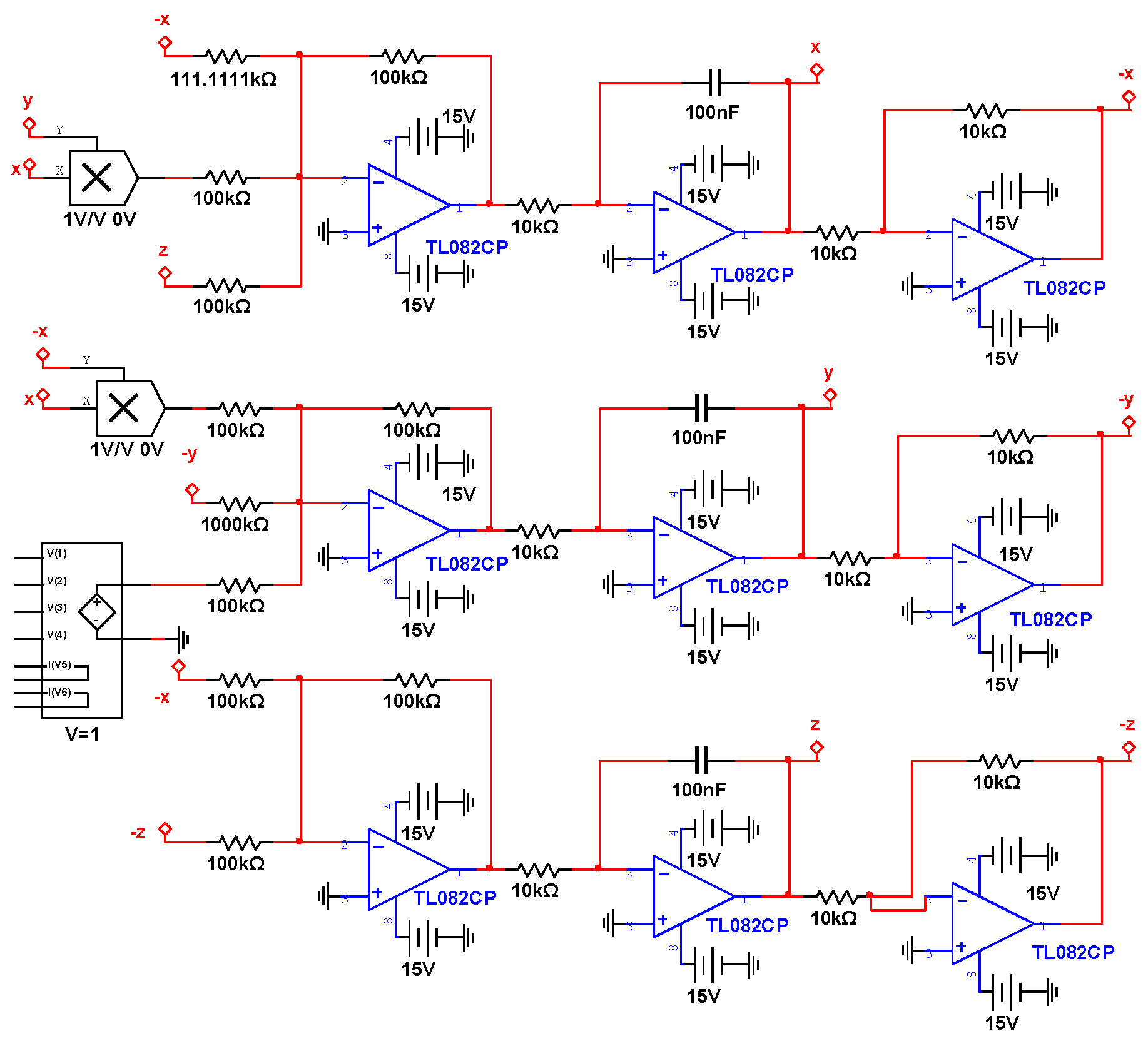
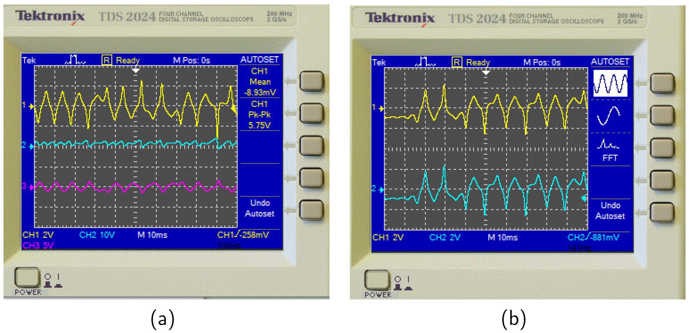
5. Circuit Implementation

In this section, the circuit implementation of the financial system and the synchronization of the master–slave systems with known and unknown parameters are designed and achieved through the software of Multisim 14.0. The specific circuit designs are given as follows.

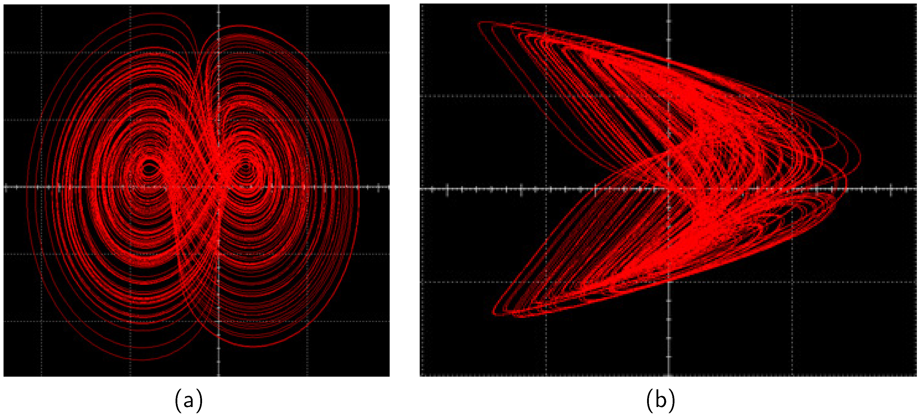
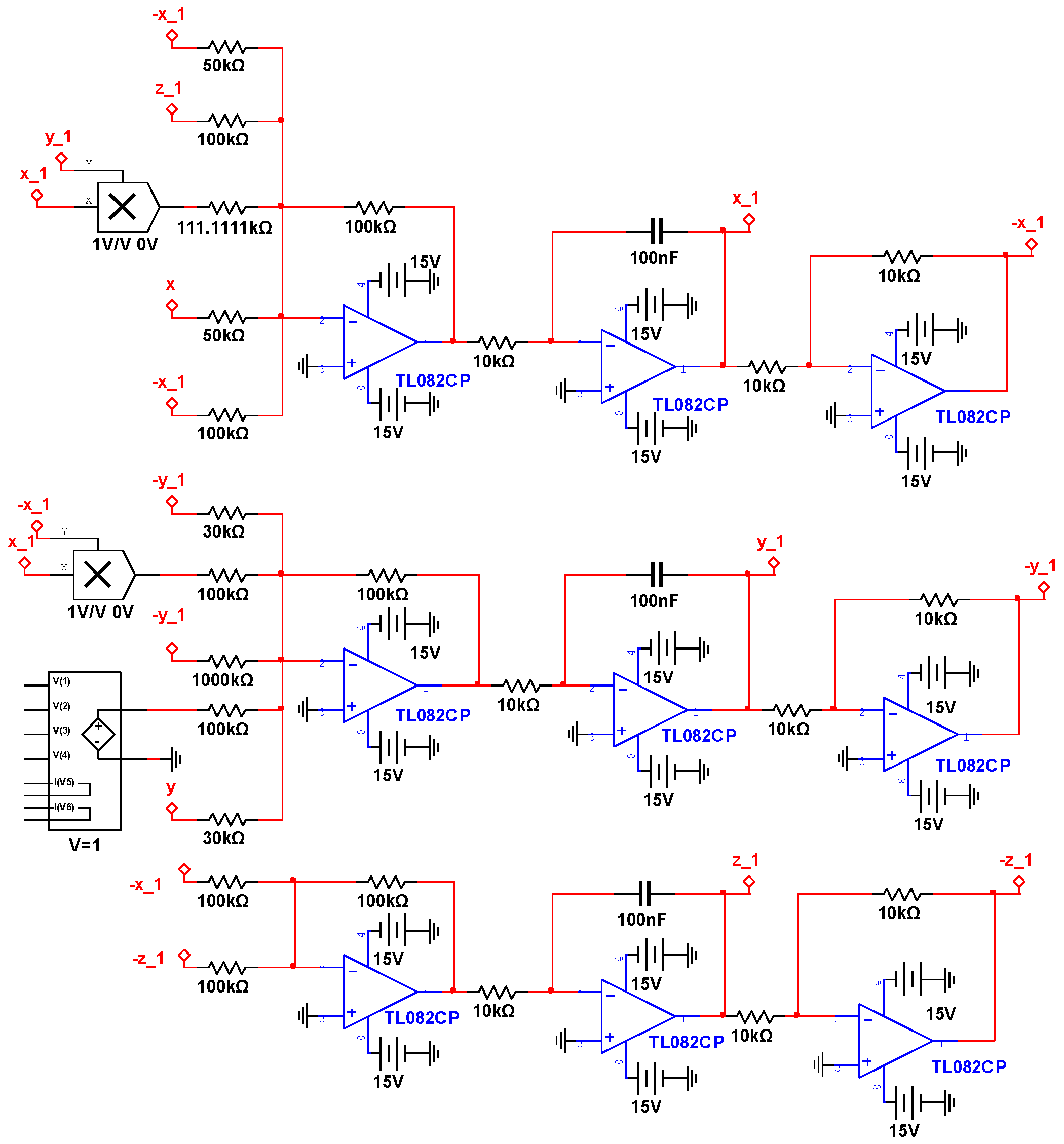
5.1. Circuit Implementation of the Financial System

Based on the circuit implementation of Multisim 14.0, the circuit of system (1) is given in Figure 11. The circuit consists of resistors, capacitors, power supplies, operational amplifiers, and multipliers. Generally, it is not easy to directly design a circuit to implement the behavior of a complex system, as the circuit implementation needs to be designed based on the specific system characteristics and the allowable range of circuit components. Due to the fact that the maximum value of the trajectory variables $x,y$, and z of the financial system (1) are all less than 5, and the voltage of the power supply is 15 volts, there is no need to make scale changes for the variables $x,y$, and z, i.e., the circuits of system (1) can be directly designed based on the system equations.

In Figure 11, the TL082CP denotes the dual input general-purpose operational amplifier, which is produced by IPC-2221A/2222, and it is used to solve the differential equations. For example, in order to implement the first differential equation $\dot{x}=z+(y-0.9)x$ in system (1) using the circuit, three operational amplifiers of the TL082CP in Figure 11 are used to simulate the operations of the model, i.e., the differential variable $\dot{x}=$$-100x/111.111+100xy/100+100z/100$. Similarly, the circuits of other systems are designed based on this principle.

According to the circuit implementation of financial system (1) in Figure 11, the waveform diagram of the variables $x,y$, and z in the oscilloscope of the circuit implementation is given in Figure 12a, and the attractor of system (1) based on the oscilloscope of the circuit implementation is shown in Figure 13 when $c=1$. Obviously, the financial system (1) is in a state of chaos. Furthermore, the attractor of system (1) based on the oscilloscope of the circuit implementation is given in Figure 14 when $c=2$, and it is in a state of period. Therefore, one can easily control the behavior of system (1) using the demand elasticity of the commodity c, and the results of the circuit implementation have once again verified the simulation results in Figure 1 and Figure 3.

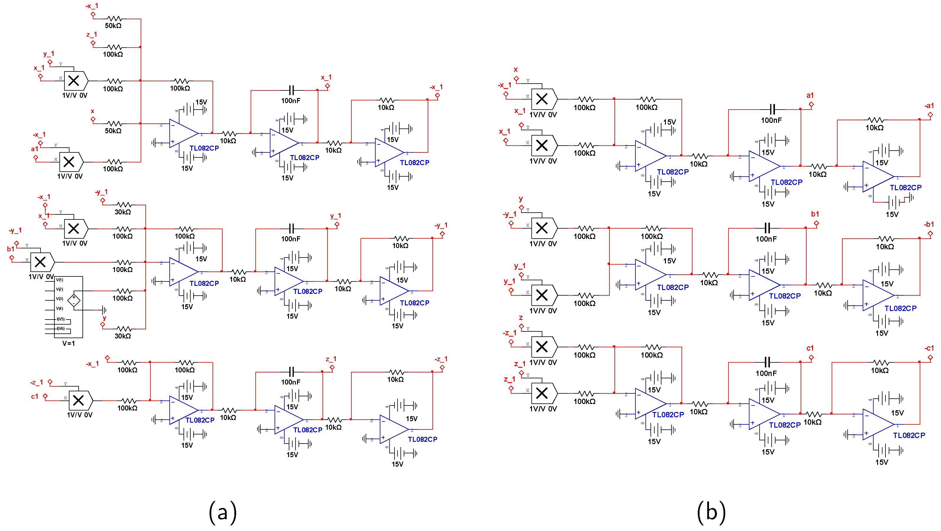
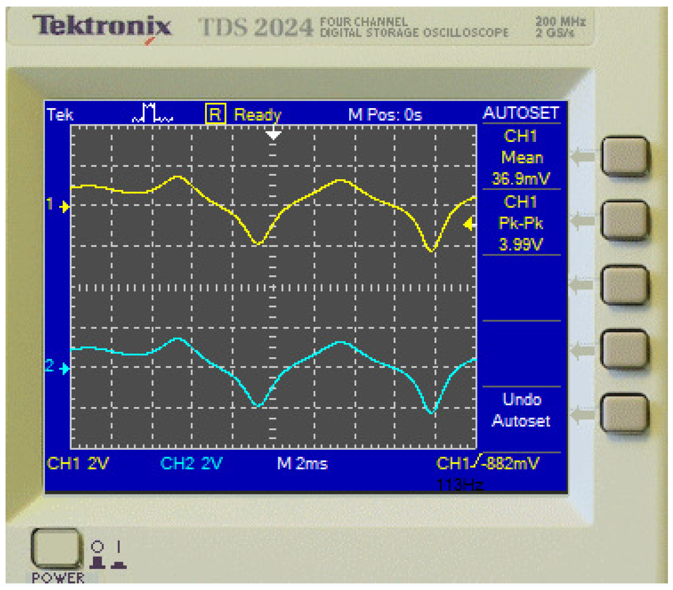
5.2. Circuit Implementation of Master–Slave Systems

Meanwhile, the circuit of slave system (3) is given in Figure 15, and only variables $x,y$ of the master system are transmitted and used to synchronize the slave system. In Figure 12b, the consensus results of the master–slave systems are shown based on Multisim 14.0. Obviously, the variable $x_1$ of slave system (3) is synchronized with the variable x of master system (1).

5.3. Circuit Implementation of Master–Slave Systems with Unknown Parameters

Meanwhile, in order to obtain the consensus of master–slave systems with unknown parameters, the circuit implementation of slave system (6) and the adaptive laws of parameters $\widehat{a},\widehat{b},\widehat{c}$ are given in Figure 16a and Figure 16b, respectively. Obviously, only variables $x,y$ of master system (1) are used to synchronize the slave system (6). The variables x vs. $x_1$ of the master–slave systems are shown in Figure 17, and the variable $x_1$ of slave system (6) is synchronized with the variable x of master system (1).

Remark 6.

The circuit implementations for the consensus of two master–slave systems are shown, as the circuit design for the consensus of multi-agent systems is similar to that of two master–slave systems, so it is not added due to space limitation.

6. Conclusions

The state of financial system can be changed from chaos to period via the parameter c, i.e., it is in a periodic state when $c=2$, and the bifurcation results show the control effectiveness is better than parameters a and b. Based on the Lyapunov stability theory, a method of master–slave systems consensus based on linear feedback control has been proposed to achieve the synchronization of financial systems with known parameters. Meanwhile, an adaptive control method has also been proposed for the consensus of master–slave systems when the parameters of the master system are unknown. Furthermore, the consensus of leader–follower multi-agent systems is also shown based on the chaotic financial systems with known parameters, and two examples of leader–follower networks are given to verify the proposed control method. The simulation results show that not only do the multi-agent systems achieve consensus, but also the unknown parameters of the master or leader systems are accurately identified. In application, the actual systems or hardware usually experience aging or deviation over time, so the adaptive control method can effectively solve the inconsistent problem caused by these unknown or uncertain parameters. Finally, the circuit implementations of the financial system, the master–slave systems, and the adaptive control laws have been designed to shown the consensus based on Multisim 14.0. The numerical experimental results and circuit implementation verify the effectiveness and feasibility of the proposed method.

References

1. Matsumoto, T.; Chua, L.; Komuro, M. The double scroll. IEEE Trans. Circuits Syst. 1985, 32, 797–818. [Google Scholar] [CrossRef]
2. Chen, G.; Ueta, T. Yet another chaotic attractor. Int. J. Bifurc. Chaos 1999, 9, 1465–1466. [Google Scholar] [CrossRef]
3. Ben Slimane, N.; Bouallegue, K.; Machhout, M. Designing a multi-scroll chaotic system by operating Logistic map with fractal process. Nonlinear Dyn. 2017, 88, 1655–1675. [Google Scholar] [CrossRef]
4. He, J.; Yu, S. Construction of higher-dimensional hyperchaotic systems with a maximum number of positive Lyapunov exponents under average eigenvalue criteria. J. Circuits Syst. Comput. 2019, 28, 1950151. [Google Scholar] [CrossRef]
5. Kuate, P.D.K.; Tchendjeu, A.E.T.; Fotsin, H. A modified rössler prototype-4 system based on Chua’s diode nonlinearity: Dynamics, multistability, multiscroll generation and FPGA implementation. Chaos Solitons Fractals 2020, 140, 110213. [Google Scholar] [CrossRef]
6. Sugandha, K.; Singh, P. Generation of a multi-scroll chaotic system via smooth state transformation. J. Comput. Electron. 2022, 21, 781–791. [Google Scholar] [CrossRef]
7. Huang, D.; Li, H. Theory and Method of the Nonlinear Economics; Sichuan University Press: Chengdu, China, 1993. [Google Scholar]
8. Xin, B.; Zhang, J. Finite-time stabilizing a fractional-order chaotic financial system with market confidence. Nonlinear Dyn. 2015, 79, 1399–1409. [Google Scholar] [CrossRef]
9. Tlelo-Cuautle, E.; Rangel-Magdaleno, J.; Pano-Azucena, A.D.; Obeso-Rodelo, P.; Nuñez-Perez, J.C. FPGA realization of multi-scroll chaotic oscillators. Commun. Nonlinear Sci. Numer. Simul. 2015, 27, 66–80. [Google Scholar] [CrossRef]
10. Yildirim, M. Optical color image encryption scheme with a novel DNA encoding algorithm based on a chaotic circuit. Chaos Solitons Fractals 2022, 155, 111631. [Google Scholar] [CrossRef]
11. Kaur, G.; Agarwal, R.; Patidar, V. Color image encryption scheme based on fractional Hartley transform and chaotic substitution–permutation. Vis. Comput. 2022, 38, 1027–1050. [Google Scholar] [CrossRef]
12. Zhao, K.; He, J. Design of higher-dimensional hyperchaotic system based on combined control and its encryption application. Int. J. Adv. Comput. Sci. Appl. 2022, 13, 869–879. [Google Scholar] [CrossRef]
13. Gámez-Guzmán, L.; Cruz-Hernández, C.; López-Gutiérrez, R.; García-Guerrero, E. Synchronization of Chua’s circuits with multi-scroll attractors: Application to communication. Commun. Nonlinear Sci. Numer. Simul. 2009, 14, 2765–2775. [Google Scholar] [CrossRef]
14. Cheng, G.; Wang, L.; Chen, Q.; Chen, G. Design and performance analysis of generalised carrier index M-ary differential chaos shift keying modulation. IET Commun. 2018, 12, 1324–1331. [Google Scholar] [CrossRef]
15. Jiang, G.P.; Tang, W.K.S.; Chen, G. A simple global synchronization criterion for coupled chaotic systems. Chaos Solitons Fractals 2003, 15, 925–935. [Google Scholar] [CrossRef]
16. Huang, C.; Cao, J. Active control strategy for synchronization and anti-synchronization of a fractional chaotic financial system. Phys. A: Stat. Mech. Its Appl. 2017, 473, 262–275. [Google Scholar] [CrossRef]
17. Aydogmus, F.; Tosyali, E. Master-slave synchronization in a 4D dissipative nonlinear fermionic system. Int. J. Control 2022, 95, 620–625. [Google Scholar] [CrossRef]
18. Kuntanapreeda, S. Adaptive control of fractional-order unified chaotic systems using a passivity-based control approach. Nonlinear Dyn. 2016, 84, 2505–2515. [Google Scholar] [CrossRef]
19. Mohadeszadeh, M.; Pariz, N. An application of adaptive synchronization of uncertain chaotic system in secure communication systems. Int. J. Model. Simul. 2022, 42, 143–152. [Google Scholar] [CrossRef]
20. Zhou, J.; Tong, D.; Chen, Q.; Zhou, W. Master-slave synchronization of neural networks with time-varying delays via the event-triggered control. Math. Comput. Model. Dyn. Syst. 2020, 26, 357–373. [Google Scholar] [CrossRef]
21. Wang, Y.; Lu, J.; Liang, J.; Cao, J.; Perc, M. Pinning synchronization of nonlinear coupled Lur’e networks under hybrid impulses. IEEE Trans. Circuits Syst. II Express Briefs 2018, 66, 432–436. [Google Scholar] [CrossRef]
22. Tang, Z.; Park, J.H.; Zheng, W.X. Distributed impulsive synchronization of Lur’e dynamical networks via parameter variation methods. Int. J. Robust Nonlinear Control 2018, 28, 1001–1015. [Google Scholar] [CrossRef]
23. Nowzari, C.; Garcia, E.; Cortés, J. Event-triggered communication and control of networked systems for multi-agent consensus. Automatica 2019, 105, 1–27. [Google Scholar] [CrossRef]
24. Huang, Y.; Bao, H. Master-slave synchronization of complex-valued delayed chaotic Lur’e systems with sampled-data control. Appl. Math. Comput. 2020, 379, 125261. [Google Scholar] [CrossRef]
25. Arena, P.; Buscarino, A.; Fortuna, L.; Patanè, L. Lyapunov approach to synchronization of chaotic systems with vanishing nonlinear perturbations: From static to dynamic couplings. Phys. Rev. E 2020, 102, 012211. [Google Scholar] [CrossRef] [PubMed]
26. Yalçin, M.E.; Suykens, J.A.; Vandewalle, J. Master-slave synchronization of Lur’e systems with time-delay. Int. J. Bifurc. Chaos 2001, 11, 1707–1722. [Google Scholar] [CrossRef]
27. Htun, Y.H.T.; Hlaing, M.S.; Hla, T.T. Master-slave synchronization of robotic arm using PID controller. Indones. J. Electr. Eng. Informatics 2023, 11, 77–87. [Google Scholar] [CrossRef]
28. Gu, Z.; Peng, S.; Huang, Y. Quasi-consensus of disturbed nonlinear multiagent systems with event-triggered impulsive control. Appl. Sci. 2022, 12, 7580. [Google Scholar] [CrossRef]
29. Trakas, P.S.; Tantoulas, A.; Bechlioulis, C.P. Formation control of nonlinear multi-agent systems with nested input saturation. Appl. Sci. 2024, 14, 213. [Google Scholar] [CrossRef]
30. Yang, J.; Lee, B.G. Distributed adaptive tracking control of hidden leader-follower multi-agent systems with unknown parameters. Mathematics 2024, 12, 1013. [Google Scholar] [CrossRef]
31. Gu, R.; Sun, X. Fault-tolerant cooperative control of multiple uncertain Euler-Lagrange systems with an uncertain leader. Electronics 2024, 13, 2068. [Google Scholar] [CrossRef]
32. Ding, K.; Han, Q.L. Master-slave synchronization criteria for horizontal platform systems using time delay feedback control. J. Sound Vib. 2011, 330, 2419–2436. [Google Scholar] [CrossRef]
33. Wen, G.; Wan, Y.; Cao, J.; Huang, T.; Yu, W. Master-slave synchronization of heterogeneous systems under scheduling communication. IEEE Trans. Syst. Man Cybern. Syst. 2016, 48, 473–484. [Google Scholar] [CrossRef]
34. Ramirez, J.P.; Garcia, E.; Alvarez, J. Master-slave synchronization via dynamic control. Commun. Nonlinear Sci. Numer. Simul. 2020, 80, 104977. [Google Scholar] [CrossRef]
35. Dadras, S.; Momeni, H.R. Control of a fractional-order economical system via sliding mode. Phys. A Stat. Mech. Its Appl. 2010, 389, 2434–2442. [Google Scholar] [CrossRef]
36. Jajarmi, A.; Hajipour, M.; Baleanu, D. New aspects of the adaptive synchronization and hyperchaos suppression of a financial model. Chaos Solitons Fractals 2017, 99, 285–296. [Google Scholar] [CrossRef]
37. Jäntschi, L. Eigenproblem basics and algorithms. Symmetry 2023, 15, 2046. [Google Scholar] [CrossRef]
38. Parks, P.C. AM Lyapunov’s stability theory–100 years on. IMA J. Math. Control Inf. 1992, 9, 275–303. [Google Scholar] [CrossRef]
39. Sastry, S.; Sastry, S. Lyapunov stability theory. In Nonlinear Systems: Analysis, Stability, and Control; Springer: Berlin/Heidelberg, Germany, 1999; pp. 182–234. [Google Scholar]
Figure 1. Attractor of financial system (1). (a) Phase diagram of x vs. y. (b) Phase diagram of y vs. z.
Applsci 14 08894 g001
Figure 2. Bifurcation diagram and Lyapunov exponent spectrum of financial system (1) with c. (a) Bifurcation diagram. (b) Lyapunov exponent spectrum.
Applsci 14 08894 g002
Figure 3. Attractor of financial system (1) with c = 2 . (a) Phase diagram of x vs. y. (b) Phase diagram of y vs. z.
Applsci 14 08894 g003
Figure 4. Errors e x , e y , e z of master–slave systems (1) and (3).
Applsci 14 08894 g004
Figure 5. Numerical simulation results of the consensus of master–slave systems (1) and (6) with unknown parameters. (a) Errors e x , e y , e z of master–slave systems (1) and (6). (b) The adaptive tracking results of parameters a ^ , b ^ , c ^ in slave system (6).
Applsci 14 08894 g005
Figure 6. The network structure of leader–follower multi-agent. (a) Five agents in Example 3. (b) Six agents in Example 4.
Applsci 14 08894 g006
Figure 7. The numerical simulation results of leader-follower systems in Example 3. (a) The errors of multi-agent systems. (b) The parameters estimation of multi-agent systems.
Applsci 14 08894 g007
Figure 8. The numerical simulation results of leader–follower systems in Example 4. (a) The errors of multi-agent systems. (b) The parameters estimation of multi-agent systems.
Applsci 14 08894 g008
Figure 9. Costs of all agents in Example 3. (a) The control costs of | k i j ( x ) ( x i x j ) | + | k i j ( y ) ( y i y j ) | + | k i j ( z ) ( z i z j ) | . (b) The costs of parameter adaptive laws | a ^ ˙ j | , | b ^ ˙ j | , | c ^ ˙ j | in Equation (18).
Applsci 14 08894 g009
Figure 10. Control costs of leader–follower agents 3 and 5 in Example 4. (a) The control costs of | k i j ( x ) ( x i x j ) | + | k i j ( y ) ( y i y j ) | + | k i j ( z ) ( z i z j ) | . (b) The costs of parameter adaptive laws | a ^ ˙ j | , | b ^ ˙ j | , | c ^ ˙ j | in Equation (18).
Applsci 14 08894 g010
Figure 11. Circuit implementation of financial system (1) based on Multisim 14.0.
Applsci 14 08894 g011
Figure 12. The results of circuit implementation of the consensus of master–slave systems (1) and (3). (a) The waveform diagrams of variables x , y , and z displayed on the oscilloscope. (b) The corresponding waveform diagrams of variables x and x 1 of the master and slave systems displayed on the oscilloscope.
Applsci 14 08894 g012
Figure 13. Attractor of financial system (1) by the circuit in Figure 11 when c = 1 . (a) Phase diagram x vs. y. (b) Phase diagram x vs. z.
Applsci 14 08894 g013
Figure 14. Attractor of financial system (1) by the circuit in Figure 11 when c = 2 . (a) Phase diagram x vs. y. (b) Phase diagram y vs. z.
Applsci 14 08894 g014
Figure 15. Circuit implementation of slave system (3) based on Multisim 14.0.
Applsci 14 08894 g015
Figure 16. Circuit implementation of the consensus of master–slave systems with unknown parameters. (a) Circuit implementation of slave system (6). (b) The adaptive laws of parameters a ^ , b ^ , c ^ in system (6).
Applsci 14 08894 g016
Figure 17. The waveform diagrams of variables x and x 1 displayed on the oscilloscope of the master–slave systems (1) and (6), respectively.
Applsci 14 08894 g017