A Novel Optimal Sensor Placement Framework for Concrete Arch Dams Based on IAHA Considering the Effects of Cracks and Elastic Modulus Degradation

Abstract

Optimal sensor placement (OSP) for arch dams is important to ensure their long-term service, but the evolution of structural states and material properties is less considered at present. This paper considers the effects of cracks, contraction joints, and elastic modulus zoning degradation of dam bodies, proposing an OSP framework based on an improved artificial hummingbird algorithm (IAHA). First, considering the compressibility of reservoir water, a finite element model of the arch dam–reservoir–foundation system is established. Second, by introducing improved circle chaotic mapping and Levy flight, IAHA is proposed. Then, a method for selecting the optimal number of sensors (ONS) based on modal assurance criterion (MAC), fitness values, and maximum singular value ratio (S) criteria is proposed. Finally, an OSP framework for arch dams with cracks is constructed and verified through a concrete arch dam. The final sensor placement is carried out for the current state of this arch dam after 45 years of operation, and the ONS is selected to give the results of the spatial location of the sensors. The results indicate that the OSP performance of the arch dam based on IAHA is the best, with MAC-MAX, MAC-AVE, MAC-RMS, and S values of 0.1521, 0.1069, 0.5478, and 1.8591, respectively, showing the best performance among the selected algorithms. The method of selecting the ONS based on MAC, fitness values, and S criteria is reasonable and feasible, considering that the changes in structural states and material properties have varying degrees of influence on the number and spatial location of sensors. The research results of this paper can provide effective technical support for the health diagnosis of arch dams with cracks and provide references and new ideas for structural health monitoring.

1. Introduction

Dams are subject to water pressure, temperature, and cumulative damage during long-term service [1,2]. Once damage occurs, it will have negative impacts on the life and property downstream of the reservoir and the environment, etc. Therefore, conducting reliability analysis and safety evaluation studies after the completion of the dam is essential to assess the overall structural safety [3,4]. Structures may suffer damage under different loads, leading to a loss of mass and stiffness and causing changes in the dynamic characteristics of the structure [5,6]. As a result, structural modal identification has become a core technology for the dynamic testing and online monitoring of modern complex engineering structures [7,8,9]. In modal testing, improper sensor placement may affect the identification of modal parameters, so it is particularly important to determine the optimal number and locations of sensors for the structure. In traditional dam dynamic tests, sensor placement is based on engineering experience, which does not guarantee the optimal placement of sensors [10,11,12]. Therefore, the study of OSP for concrete arch dams has become an important topic [13,14].

1.1. Literature Review

Since the issue of OSP was raised, numerous scholars have studied and proposed many classical methods. In 1991, Kammer [15] proposed the effective independence (EI) method, which achieved the best estimation of modal parameters with as few sensors as possible by eliminating test points that contribute less to the target modal partitions among the candidate points. Salama et al. [16] proposed the modal kinetic energy (MKE) method, which arranged the measuring points in each degree of freedom (DOF) of the structure in the order of modal kinetic energy to select the sensor locations with larger vibration energy. Li et al. [17] compared the intrinsic connection between the modal kinetic energy (MKE) method and the effective independence (EI) method, proposing an alternative form of the two effective computational iterative EI methods. Meo et al. [18] demonstrated that the effective independence driving-point residue (EI-DPR) method provided an effective method for OSP in identifying the vibration characteristics of bridges by studying six different sensor placement techniques. Li et al. [19] proposed a fast and efficient independence method based on QR decomposition, which greatly improved the computational efficiency without the need to compute the information matrix of the structure. Zhang et al. [20] proposed a novel multi-factor OSP strategy, namely, effective independence-acceleration amplitude-total displacement (EI-AA-TD), to formulate a multifactor optimization framework for sensor placement. The above classical methods are effective, but often the results obtained are not optimal solutions.

Various intelligent algorithms have been applied to OSP to address the shortcomings of some classic algorithms [21]. He and Xing et al. [22] proposed an improved adaptive genetic algorithm (IAGA) based on the modified modal assurance criterion and verified the effectiveness of the method in sensor placement for a wharf structure. Yi et al. [23] introduced an adaptive monkey algorithm (AMA) to solve the sensor placement problem for target locations under the constraints of computational efficiency and convergence stability. Qin et al. [24] proposed an improved partheno-genetic algorithm (IPGA) based on the initial layout of sensors and applied it to a quayside container crane. Nicoletti et al. [25] chose an evolutionary optimization algorithm (EOA) based on particle swarm optimization (PSO) and validated it through a 4-story tall RC building, a footbridge, and a historic masonry church damaged by earthquake actions. Kord et al. [26] proposed a novel triple-structure coding approach and implemented the encoding scheme using two of the most famous evolutionary algorithms, the genetic algorithm (GA) and the mutated particle swarm optimization (MPSO) algorithm, to address the practicality of modal identification in high-rise structures and steel dome trusses, demonstrating progress in cost reduction in the context of sensor layout optimization. Raorane et al. [27] used an exhaustive search method, a heuristic search method, and a genetic algorithm based on Bayesian optimal sensor placement strategy to determine the optimal (and worst) position of sensor clusters for AE source localization in isotropic plates with unknown material properties. To strike a balance between sensor cost and real-time performance, Ma et al. [28] proposed a new optimal sensor placement (OSP) method. A two-stage OSP method based on the hierarchical ranking evolutionary algorithm (HREA) has been developed, and four classic binary multi-objective optimization algorithms have been introduced for comparison. In addition, the AHA algorithm, although it falls under the category of meta-heuristic algorithms, is significantly different from existing algorithms. In AHA, the migratory foraging strategy ensures exploration of the search space, while the territorial foraging strategy promotes the exploitation of the search space; the guided foraging strategy emphasizes early exploration and later exploitation [29]. Therefore, considering these factors, AHA exhibits significant differences from existing algorithms. At present, the commonly used methods for initializing populations are tent chaotic mapping and logistic chaotic mapping. But both of these mappings have flaws, so they need to be improved to enhance AHA’s global search capability.

With the development of structural health monitoring technology based on modal data, scholars have made significant research progress in OSP methods for arch dams. Chen et al. [30] proposed a hybrid method that provides linear independent and orthogonal modal vectors to minimize the relative mean square error of the measured vibration modes, demonstrating the feasibility of this approach through an example of an arch dam. Cao et al. [31] introduced a distance coefficient–multi objective information fusion algorithm (D-MOIF) for sensor placement and validated its effectiveness with a high arch dam case study. Zhu et al. [7] utilized a quantum genetic algorithm (QGA) for OSP on arch dams to achieve more precise modal parameter identification. He and Lian et al. [14] incorporated grade evaluation and migration strategy and the mutation operators of the genetic algorithm into an integer-encoding particle swarm optimization algorithm (IMPSO), which was applied to OSP for the Laxiwa arch dam. Kang et al. [32] integrated the virus evolutionary theory into a genetic algorithm, proposing a virus coevolutionary partheno-genetic algorithm (VEPGA) for OSP on a portal frame and a concrete arch dam, showcasing the superiority of this algorithm. Lian et al. [33] introduced a novel fitness function derived from the nearest neighbor index, combining an improved discrete particle swarm optimization algorithm with a clonal selection algorithm (CSA-DPSO) for OSP in an arch dam.

The OSP is based on modal data, which includes modal frequencies and mode shapes that can describe the dynamic behavior of a structure system [32]. The presence of reservoir water is considered to have effects on the natural frequencies and mode shapes of the structure, leading to changes in its dynamic characteristics. In 1933, Westergaard [34] proposed an added mass formula for the dynamic water pressure of a rigid upright dam face without considering the compressibility of the reservoir water. In 1982, Clough [35] extended the added mass formula to adapt to dams of any shape and seismic accelerations in all directions. Although the added mass method is simple, it cannot accurately simulate the interaction between the dam body and reservoir water. Therefore, many scholars have studied the impact of reservoir water using the finite element method [36]. Du et al. [37] established an arch-dam–water–rock-foundation model and studied the compressibility of reservoir water on the vibration performance of arch dams, demonstrating that the presence of water reduces the system’s natural frequencies and that there are significant differences in the responses obtained from the compressible reservoir model and the Westergaard added mass model. Chopra [38] analyzed the impact of reservoir water compressibility on the dynamic characteristics of arch dams, and through a series of example analyses of actual dams, it was shown that neglecting the compressibility of water may seriously underestimate or overestimate the stresses in certain dams, considering that the compressibility of water can change the system’s natural frequencies. Wang and Zhang et al. [39] concluded that four scenarios involving setting up different combinations of foundations and impounded water models have a significant impact on a system’s natural frequencies and on the system’s fundamental frequency calculated after considering that the compressibility of the impounded water is close to the identified value.

The existing literature on OSP for arch dams is based on seamless holistic models. Consideration of cracks, contraction joints, and elastic modulus zoning degradation of a dam body also affects the dynamic characteristics and deformation behavior of arch dams to varying degrees [40,41]. Pan [42] revealed the effect of contact stiffness of contraction joints on natural frequencies of high arch dams through numerical simulation, and the results showed that the presence of contraction joints was considered to reduce natural frequencies of arch dams to a certain extent, and natural frequencies of arch dams became larger with the increase in contact elastic modulus. Yang et al. [43] compared a linear finite element model of the dam with a nonlinear model that considers contraction joints and found that when simulating the Ertan arch dam, the mode shapes and natural frequencies calculated using the nonlinear model both changed. Sevim et al. [44] constructed a prototype arch-dam–reservoir–foundation model for ambient vibration tests under laboratory conditions, and the results showed that with the increase in cracks, the natural frequencies of the dam significantly decreased. Wang and Jin et al. [45] proposed a model for simulating concrete degradation with aging caused by chemo-mechanical damage and analyzed the seismic response of arch dams with aging effects, demonstrating that the aging of arch dams leads to an increase in tensile cantilever stress, dynamic displacement, and joint opening during earthquakes. Altunisik et al. [46] established a prototype arch-dam–reservoir–foundation model in the laboratory, and through multiple experiments, it was concluded that the increase in concrete stiffness, aging, temperature, and various environmental effects are the causes of the increase in natural frequencies.

In addition, existing research often selects a rough number of sensors based on experience methods. Yi et al. [11] assumed 20 sensors for the Canton Tower. Li and Song et al. [12] selected 12 sensors for the cantilever model based on the variation curve of the maximum off-diagonal element of the MAC matrix and economic factors. Zhu et al. [7] directly assigned 30 sensors for the arch dam. He and Lian et al. [14] and Lian et al. [33] assumed that the number of sensors is not critical and directly set the number of sensors for the arch dam to be 30. Chen et al. [30] determined 20 sensors for the arch dam by plotting the variation curve of the off-diagonal element of the MAC matrix. Kang et al. [32] set the number of sensors for the arch dam to be 20.

The remaining contents of this paper are as follows. Section 2 provides a detailed introduction to the fluid–solid coupling model, simulation methods and principles for cracks, contraction joints, and elastic modulus zoning degradation of the dam body, OSP methods, evaluation criteria, and constructs an OSP framework for arch dams with cracks. Section 3 applies the OSP framework to an example of an arch dam, selects the optimal placement algorithm, and studies the impacts of structural state and material property evolution on sensor placement. Section 4 offers some conclusions.

1.2. Problem Statement

Scholars have achieved excellent results in the OSP of arch dams, but there are still some shortcomings and areas that deserve further research, such as:

(1)

Most scholars consider the role of dynamic water pressure of arch dams based on the Westergaard added mass model, which ignores the damping effect caused by the complex coupling motion of reservoir water and dam bodies, making the calculation results not accurate enough [37,38,39]. Second, the literature on the OSP problem of arch dams is mostly based on a seamless ideal model that does not consider the changes in structural states and material properties [7,14,30,31,32,33].

(2)

Intelligent algorithms can estimate modal parameters well, but it is easy to miss some points with key information in the spatial distribution, which tends to result in sub-optimal solutions [23,31], but different algorithms have differences in performance, as well as in the results of sensor layout. In addition, the selection of the number of sensors has mostly been based on the experience or sequence methods, combined with factors such as modal identification accuracy or economic considerations. This approach often results in an inaccurate estimation of the required number of sensors, leading to unsatisfactory sensor layout results [7,11,12,14,30,32,33].

1.3. Proposed Solution

The main goals of this paper are to establish a reasonable and effective FSCM (fluid–structure coupling model) for the arch dam and to study the influence of the evolution of structural states and material properties on the OSP of arch dams; the OSP method that is most suitable for the model in this paper is optimized. Therefore, this paper considers the impacts of reservoir compressibility and structural states, as well as the material properties’ evolution on the dynamic characteristics of arch dams. It improves and prefers the IAHA, proposing an optimal sensor quantity determination method based on MAC, fitness values, and S criteria. It establishes a concrete arch dam OSP framework based on IAHA, considering the effects of cracks, contraction joints, and elastic modulus zoning degradation of the dam body. The feasibility of the above method is validated through a concrete arch dam with cracks, aiming to provide technical support and new research ideas for the OSP of dams. The final sensor placement is carried out for the current state of this arch dam after 45 years of operation; the ONS is selected, and the results of the spatial location of the sensors are given. The primary contributions and innovations of this paper are as follows:

(1)

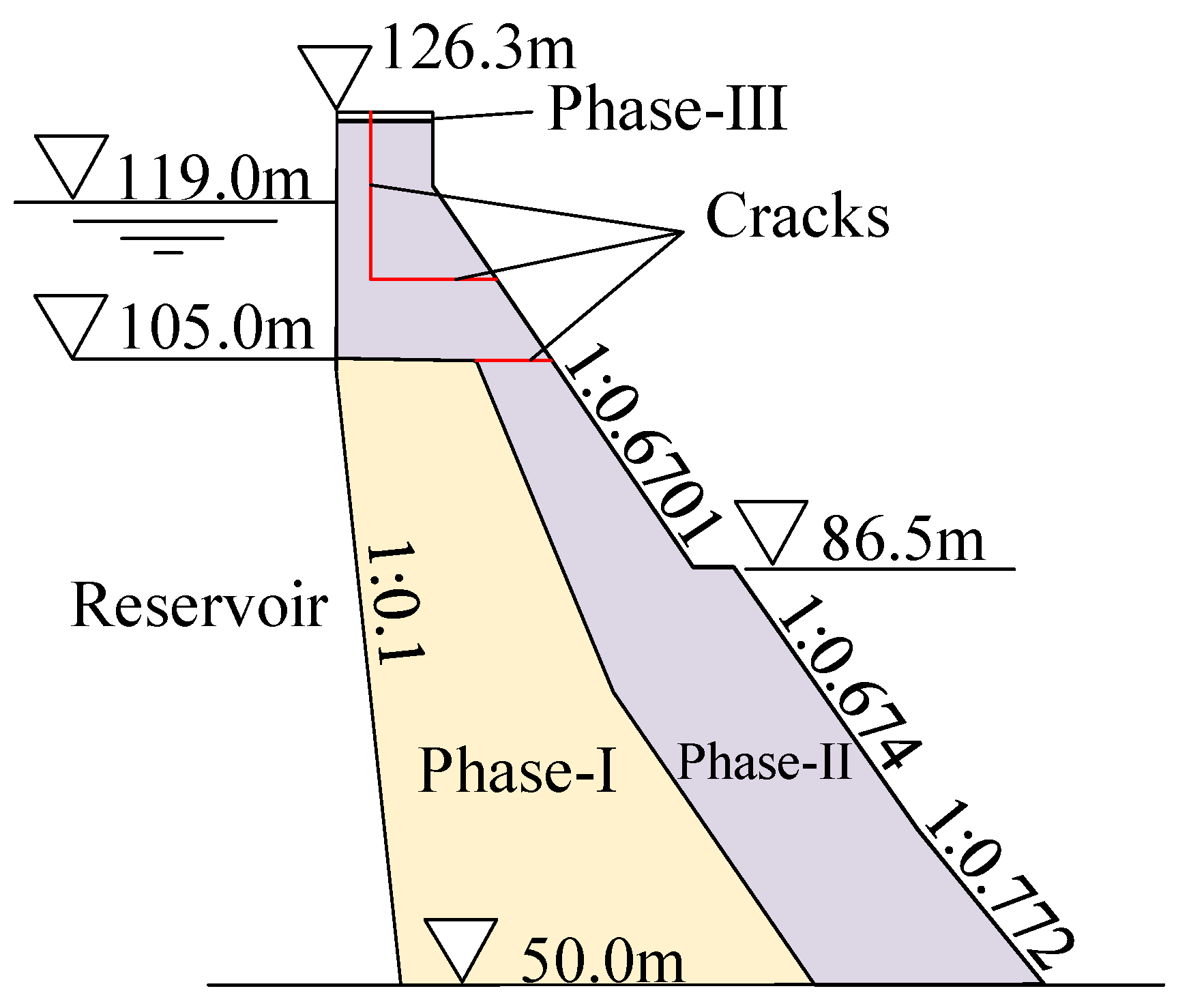
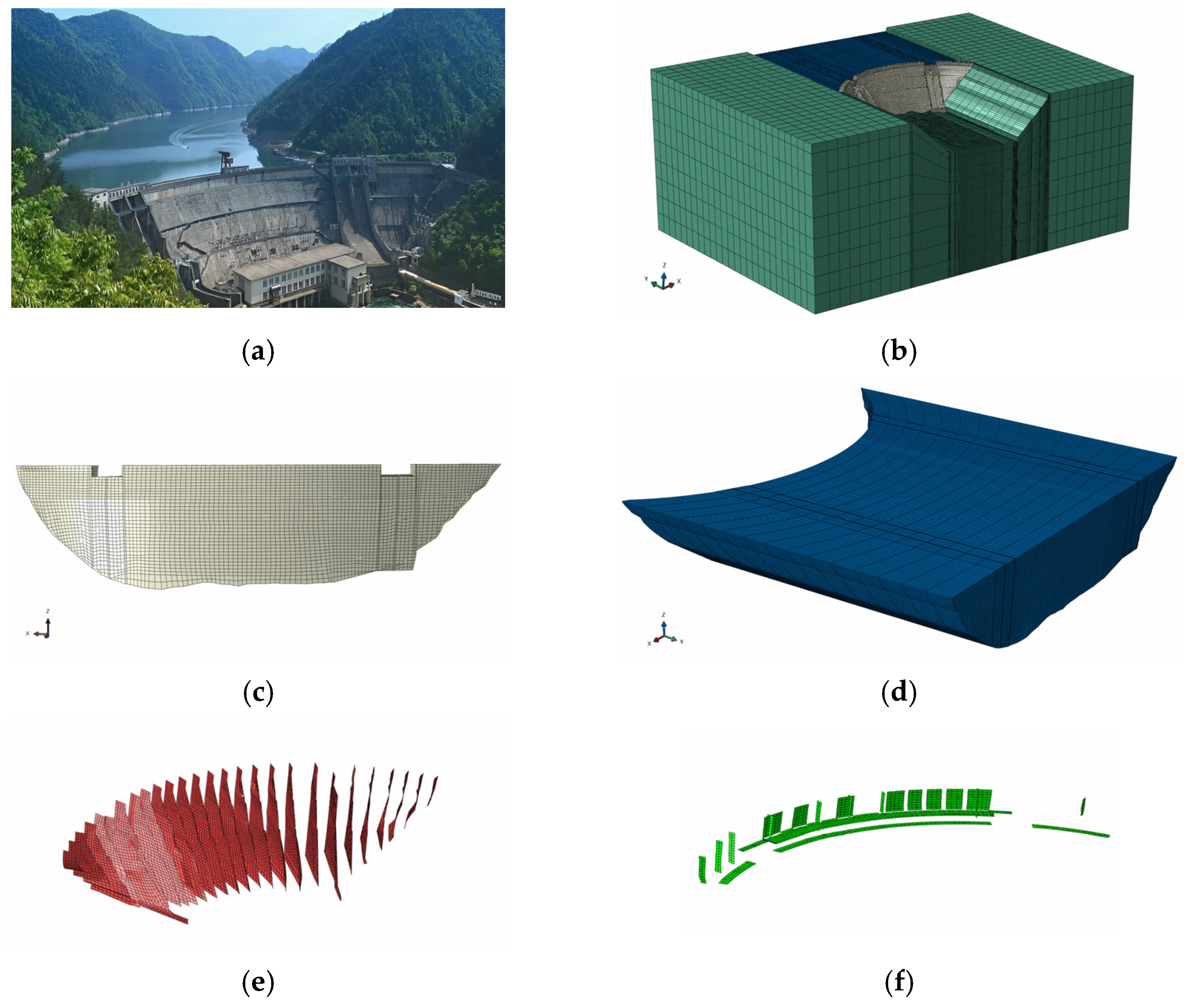
Based on FSCM and considering the compressibility of reservoir water, an arch-dam–reservoir–foundation model is established to calculate the modal data required for the OSP of an arch dam. This method considers the damping effect brought by the complex coupling motion between the reservoir water and the dam body and can provide more reasonable and realistic modal data for arch dam OSP. This investigation includes the effects of horizontal cracks, vertical cracks, contraction joints, dam body elastic modulus zoning, dam body elastic modulus zoning degradation, and combinations of these factors on the OSP of the arch dam.

(2)

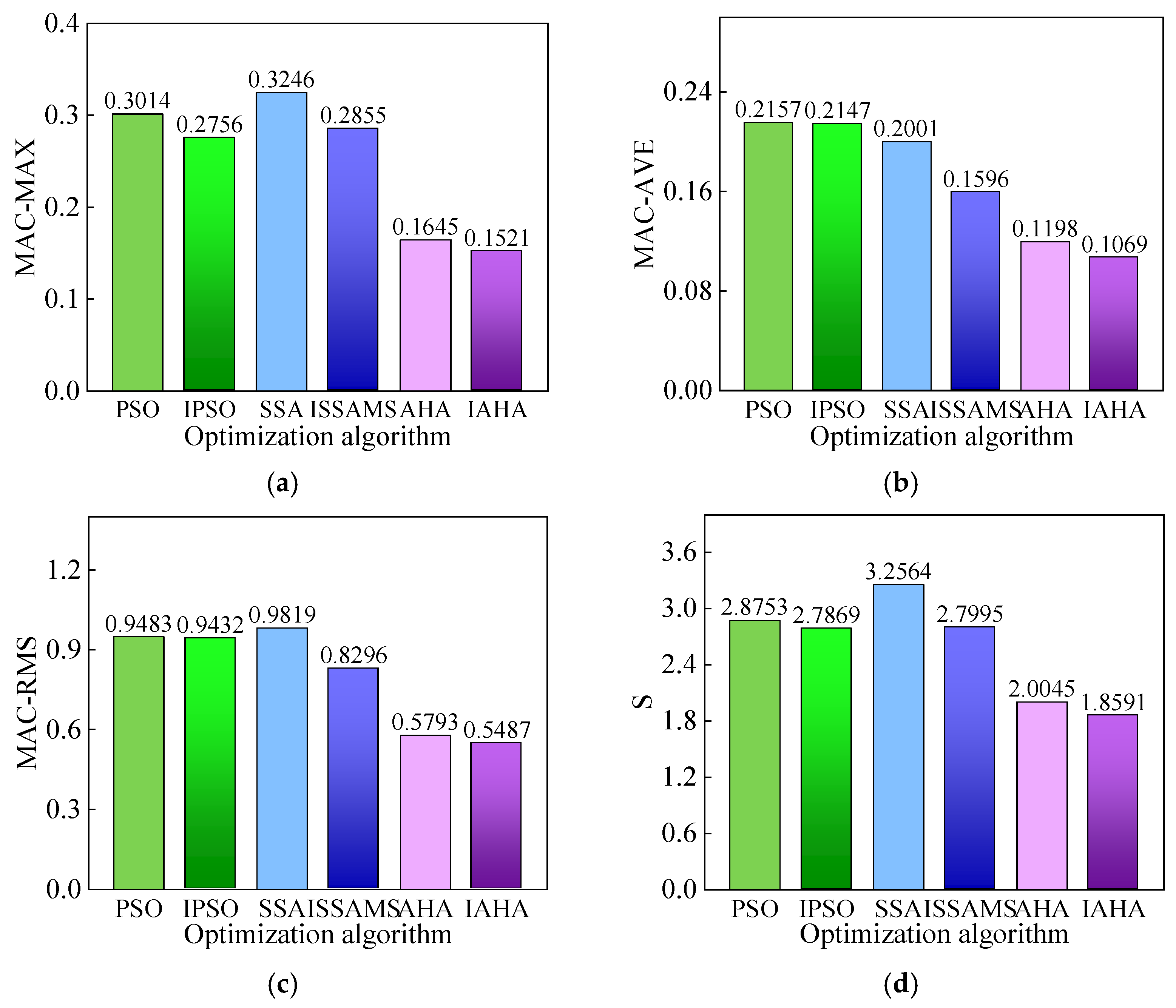
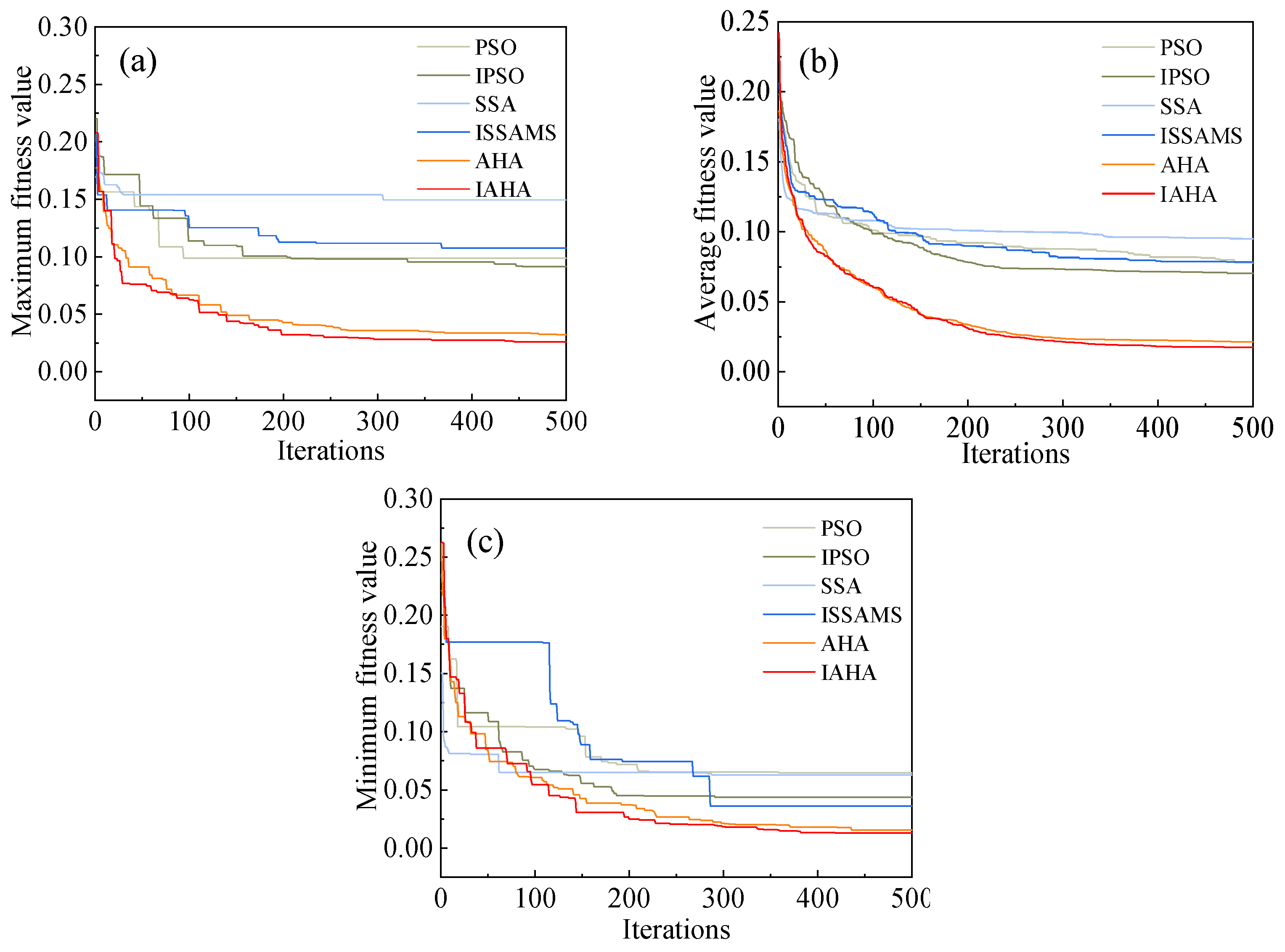
An IAHA is proposed and compared with five intelligent algorithms to verify its superiority in performance and sensor layout effectiveness, providing a new intelligent algorithm for the OSP problem of hydraulic structures. A method for selecting the ONS based on MAC, fitness values, and S criteria is proposed that can accurately determine the ONS under different working conditions and is worth promoting in the field of OSP.

(3)

In the current state of 45 years of actual operation of the arch dam, considering factors such as cracks, contraction joints, and elastic modulus zoning degradation of the dam body, it is finally determined that the number of sensors required to be placed for the arch dam is 36, and the overall spatial position of the sensor layout is uniform and reasonable.

2. Principles and Methodologies

2.1. Arch-Dam–Reservoir–Foundation Simulation Method

2.1.1. Westergaard Added Mass Model

The Westergaard added mass model is generalized by Clough to apply to dam faces of arbitrary shape and to seismic accelerations in all directions [34,35]. It is formulated as follows:

$$M_i={\displaystyle \frac{7}{8}}\rho A_i\sqrt{H_0{h}_i}{l}_i^{⊺}{l}_i$$

(1)

where M_i is the added mass at point i on the dam surface, $\rho$ is the density of water, A_i is the area of influence at point i, h_i is the water depth at the point i, and l_i is the vector normal to the point i.

2.1.2. Fluid–Solid Coupling Model (FSCM)

The fluid–solid coupling model (FSCM) assumes that the reservoir water is a uniform, inviscid, irrotational, and compressible ideal fluid, and the dynamic water pressure generated by the reservoir water vibration satisfies the following wave equation [39]:

$${\nabla }^{2}p\left(x,t\right)-{\displaystyle \frac{1}{c^2}}{\displaystyle \frac{{\partial }^{2}p}{\partial t^2}}=0$$

(2)

where $\nabla$ is the Laplace differential operator, c is the acoustic wave velocity in the water, $p$ is the dynamic water pressure, and $t$ is time.

The boundary conditions of the coupled dam reservoir-water flow-solid system are categorized into the following four main types:

(1)

Free surface boundary conditions

Without considering the free surface micro-amplitude gravity waves, the boundary condition of the reservoir water surface can be expressed as:

$$p=0$$

(3)

(2)

Fluid–solid coupling boundary conditions

$${\displaystyle \frac{\partial p}{\partial n}}=-{\rho }_w{\ddot{u}}_n$$

(4)

where $n$ is the outer normal direction of the fluid domain at the dam–reservoir interface, ${\rho }_w$ is the density of the water, and ${\ddot{u}}_n$ is the normal absolute acceleration.

(3)

Radiation boundary conditions at the end of the reservoir

At the tail end of the reservoir, sufficiently far from the dam to satisfy the no-reflection condition:

$${\displaystyle \frac{\partial p}{\partial n}}=-{\displaystyle \frac{1}{c}}{\displaystyle \frac{\partial p}{\partial t}}$$

(5)

(4)

Absorption boundary conditions at the bottom of the reservoir

At the bottom boundary of the reservoir, the following boundary conditions are satisfied without considering the influence of the sediment adsorption boundary at the bottom of the reservoir:

$${\displaystyle \frac{\partial p}{\partial n}}=0$$

(6)

2.2. Simulation Methods for Cracks, Contraction Joints, and Degradation of Elastic Modulus

When simulating the dynamic characteristics of concrete arch dams, cracks, contraction joints, and the degradation of elastic modulus are key factors affecting the dynamic behavior of the arch dam. To accurately capture the impact of these characteristics on the dynamic response of the arch dam, this study employs the numerical calculation methods described in detail from Section 2.2.1, Section 2.2.2 and Section 2.2.3. The combined use of these methods provides an integrated numerical simulation framework for the cracks, contraction joints, and material performance degradation of the arch dam, thereby providing the necessary foundation for the subsequent optimal sensor placement. Below is a detailed introduction to these methods.

2.2.1. Simulation of Horizontal and Vertical Cracks

This paper uses cohesive elements to simulate the horizontal and vertical cracks of the arch dam. In the linear elastic stage, the stress-strain relationship is expressed as:

$$\left.t=\left\{\begin{array}{c}{t}_n\\ t_s\\ t_t\end{array}\right.\right\}=\left[\begin{array}{ccc}{E}_{nn}& E_{ns}& E_{nt}\\ E_{ns}& E_{ss}& E_{st}\\ E_{nt}& E_{st}& E_{tt}\end{array}\right]\left\{\begin{array}{c}{\epsilon }_n\\ {\epsilon }_s\\ {\epsilon }_t\end{array}\right\}$$

(7)

$${\epsilon }_n={\displaystyle \frac{{\delta }_n}{T_0}},\hspace{1em}{\epsilon }_s={\displaystyle \frac{{\delta }_s}{T_0}},\hspace{1em}{\epsilon }_t={\displaystyle \frac{{\delta }_t}{T_0}}$$

(8)

where $t_{n\left(s,t\right)}$ represents traction force, ${\delta }_{n\left(s,t\right)}$ represents the separation amount of the upper and lower surfaces of the cohesive element, and $T_0$ represents the thickness of the element.

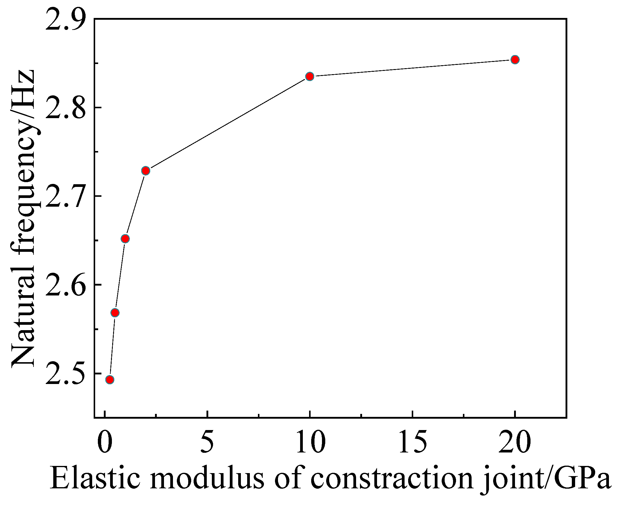
2.2.2. Simulation of Contraction Joints

Eigenvalue problems can be utilized to determine the natural frequency of undamped systems [42]:

$$\left(\begin{array}{c}-{\omega }^{2}M+K\end{array}\right)\varphi =0$$

(9)

where $M$ is the mass matrix, $K$ is the stiffness matrix, $\varphi$ is the eigenvector, and $\omega$ is the natural circular frequency.

For arch dams with contraction joints, when simulating the interaction of contraction joints using surface-to-surface contact, the system’s stiffness matrix comprises two parts: the dam body stiffness matrix and the contraction joint stiffness matrix:

$$K=K_{\mathrm{dam}}+K_{\mathrm{joint}}$$

(10)

where $K_{\mathrm{dam}}$ and $K_{\mathrm{joint}}$ are the stiffness matrix of dam body and contraction joints, respectively.

Defining the relationship between contraction joint contact force p and penetration h:

$$p=p(h)$$

(11)

This paper employs surface-to-surface contact to simulate the interaction of contraction joints and assumes that the contact relationship of contraction joints follows a piecewise linear relationship, namely:

$$p=\left\{\begin{array}{cc}kh& ,h<h_0\\ k{h}_0+10k(h-h_0)& ,h\ge h_0\end{array}\right.$$

(12)

where k is the elastic modulus of the contraction joint, and h₀ is the penetration at that point.

2.2.3. Simulation of Degradation of Elastic Modulus

Due to the influence of factors such as chemistry and mechanics, the performance parameters of concrete materials are not stable and often undergo degradation over time [47]. Nik Zainab et al. [48] proposed a mathematical equation for the time-dependent degradation of the elastic modulus of concrete as:

$$E_m(t_a)=0.0175t_a^3-3.4054t_a^2+29.807t_a+E_m$$

(13)

where $t_a$ represents the degradation duration in years, $E_m$ is the initial elastic modulus of concrete in MPa, and $E_m(t_a)$ is the degraded elastic modulus of concrete in MPa.

2.3. OSP Methods

After determining the methods for simulating the dynamic characteristics of arch dam structures, the next step is to effectively arrange sensors to monitor the health condition of the arch dam. This section will provide a detailed introduction to the methods and evaluation criteria used for the optimal sensor placement on arch dams, including the selection of intelligent algorithms, the determination of target modes, the choice of sensor quantity, and their spatial distribution, as well as the evaluation of the placement results. Through these methods, the sensor placement scheme will ensure efficient capture of the arch dam’s dynamic characteristics while considering the complexity of the structure and the monitoring requirements. The specific methods and procedures are described as follows.

2.3.1. Intelligence Algorithms

The artificial hummingbird algorithm (AHA) is a novel metaheuristic optimization algorithm proposed by Zhao et al. in 2021 [49]. At present, the commonly used methods for initializing populations are tent chaotic mapping and logistic chaotic mapping. The uneven distribution of traditional logistic chaotic mapping has an impact on the convergence speed and accuracy of the algorithm. Although tent mapping has a more uniform distribution, it has unstable periods and is prone to getting stuck in fixed points. Circle mapping is relatively stable and has a distribution uniformity comparable to tent. Specific evidence can be found in reference [50]. This paper utilizes an improved circle chaotic mapping for initializing the population to enhance the global search capability of the initial population. The improved circle mapping addresses the issues of uneven distribution and unstable periodicity that exist in traditional logistic and tent chaotic mapping. The specific formula is as follows:

$$X_{i+1}=\mathrm{mod}\left[3.14X_i+0.6-\left({\displaystyle \frac{0.65}{3.14\pi }}\right)\sin \left(3.14\pi X_i\right),1\right]$$

(14)

where X_i+1 represents the (i + 1)-th position, the X_i position is known, the (i + 1)-th position is obtained by the remainder of its operation, and mod is the remainder function.

Next, during the foraging process, Levy flight is incorporated to expand the search space [51], guiding foraging or territory foraging and updating the food source positions of the artificial hummingbirds to avoid premature convergence. The position update formula is given by:

$$x_i(t+1)=\left\{\begin{array}{ll}{x}_i(t)+\alpha \oplus Levy(\lambda )\hfill & f(x_i(t))\le f(v_i(t+1))\hfill \\ v_i(t+1)\hfill & f(x_i(t))>f(v_i(t+1))\hfill \end{array}\right.$$

(15)

where $Levy(\lambda )$ represents the random search path, which satisfies:

$$Levy~u=t^{-\lambda },\hspace{1em}1<\lambda \le 3$$

(16)

The step length follows a Levy distribution, and the step length s is calculated as:

$$s={\displaystyle \frac{\mu }{|v{|}^{1/\beta }}}$$

(17)

where $\mu$ and $v$ follow a normal distribution, defined as:

$$\mu ~N(0,{\sigma }_{\mu }^2),v~N(0,{\sigma }_v^2)$$

$${\sigma }_{\mu }={\displaystyle \frac{(1+\beta )(\sin \frac{\pi \beta }{2})}{\frac{1+\beta }{2}{\beta }^2\frac{\beta -1}{2}}},{\sigma }_v=1$$

(18)

where $\beta$ is typically a constant, often set to 1.5.

Based on the above description, the flowchart of IAHA is illustrated in Figure 1.

In this paper, intelligent algorithms such as AHA [49], IAHA, the particle swarm optimization algorithm (PSO) [52], the improved particle swarm optimization algorithm (IPSO) [53], the sparrow search algorithm (SSA) [54], and the improved sparrow search algorithm (ISSAMS) [50] are used for OSP on the arch dam. By comparing and analyzing the performance of various algorithms and the effectiveness of OSP, the most suitable intelligent algorithm for the fitness function used in this paper is selected.

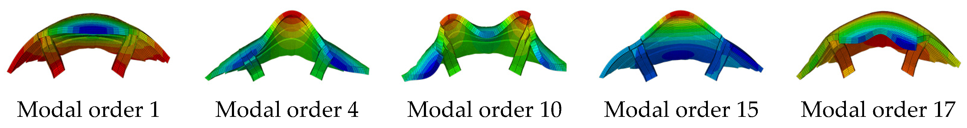
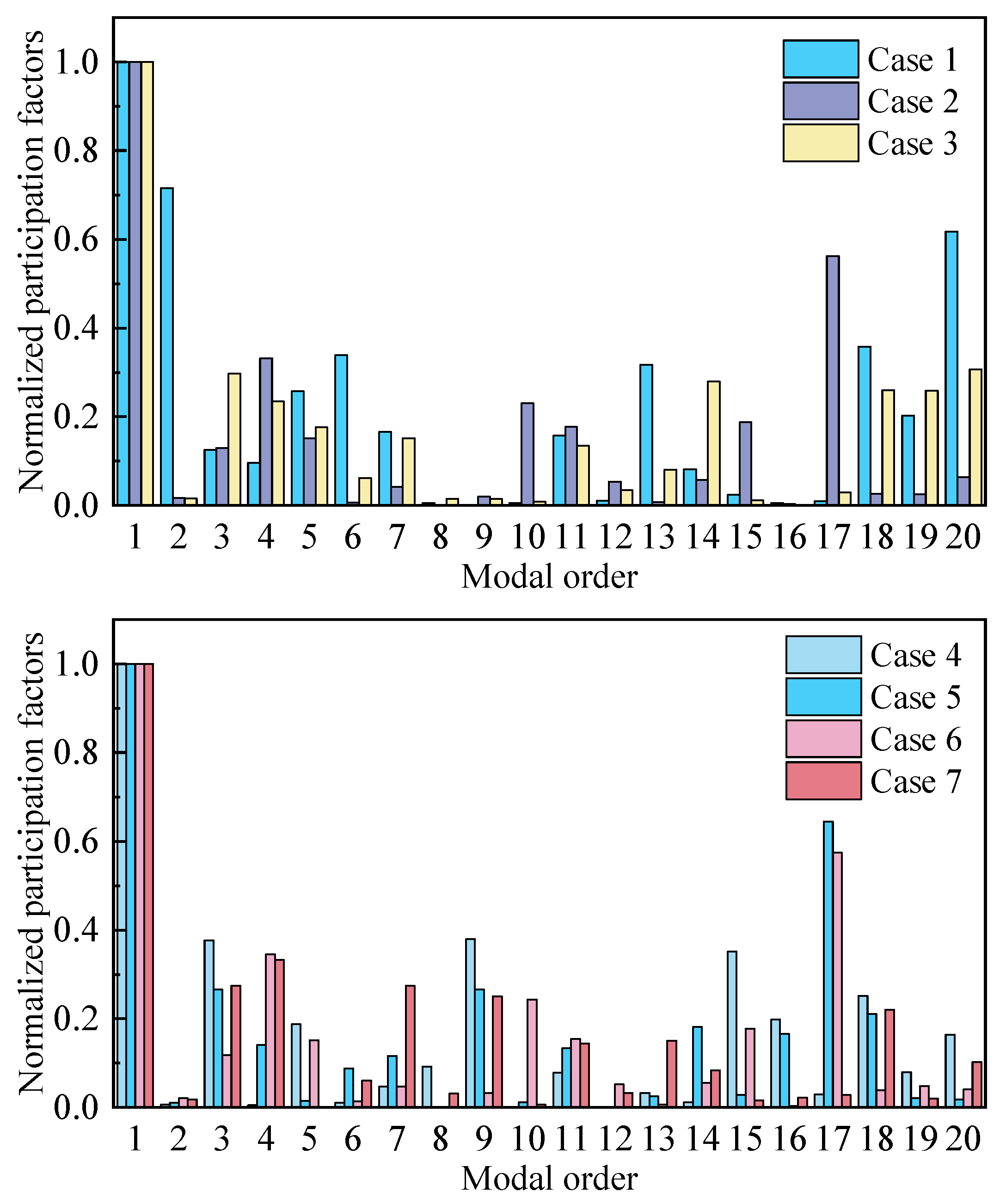
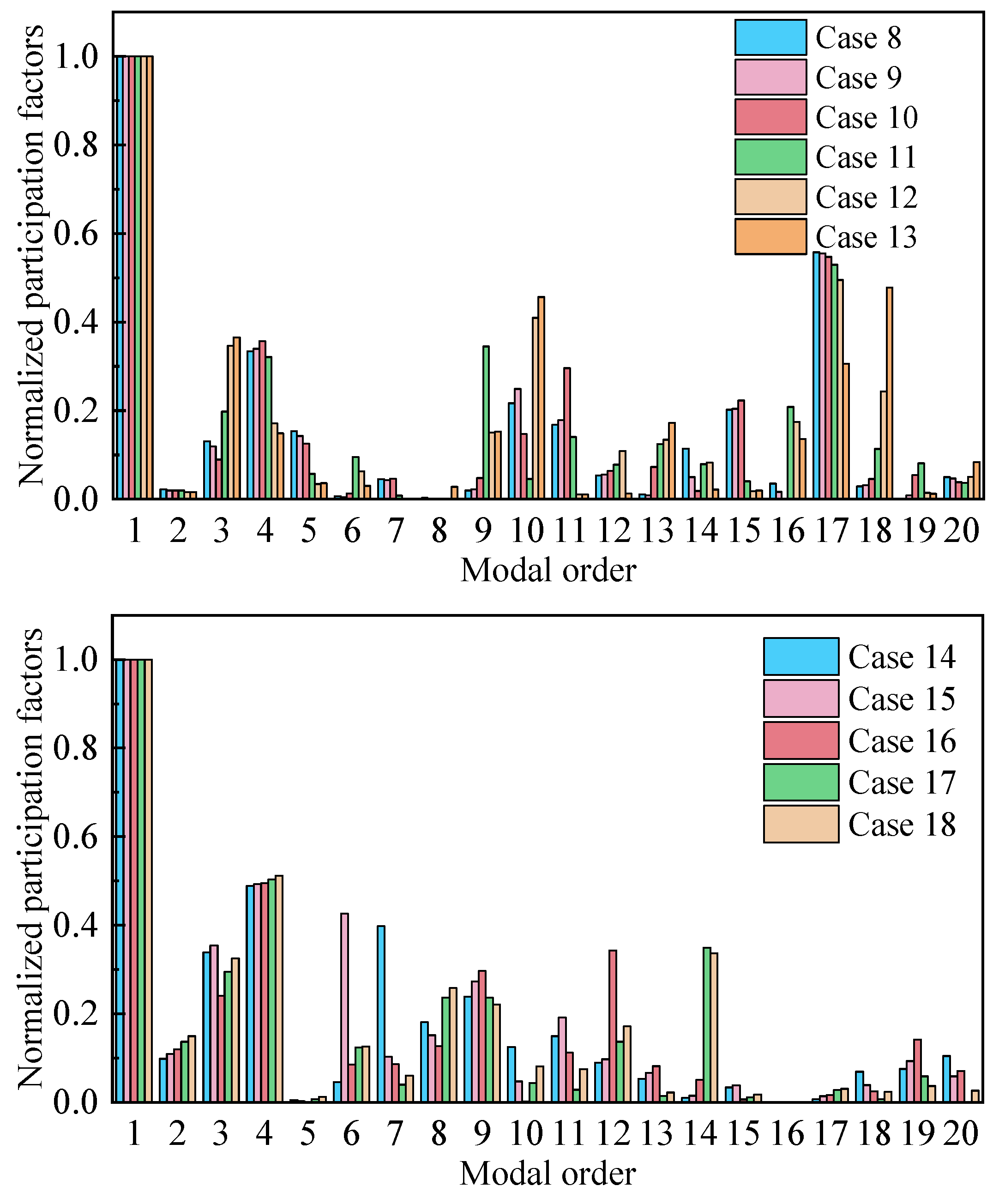
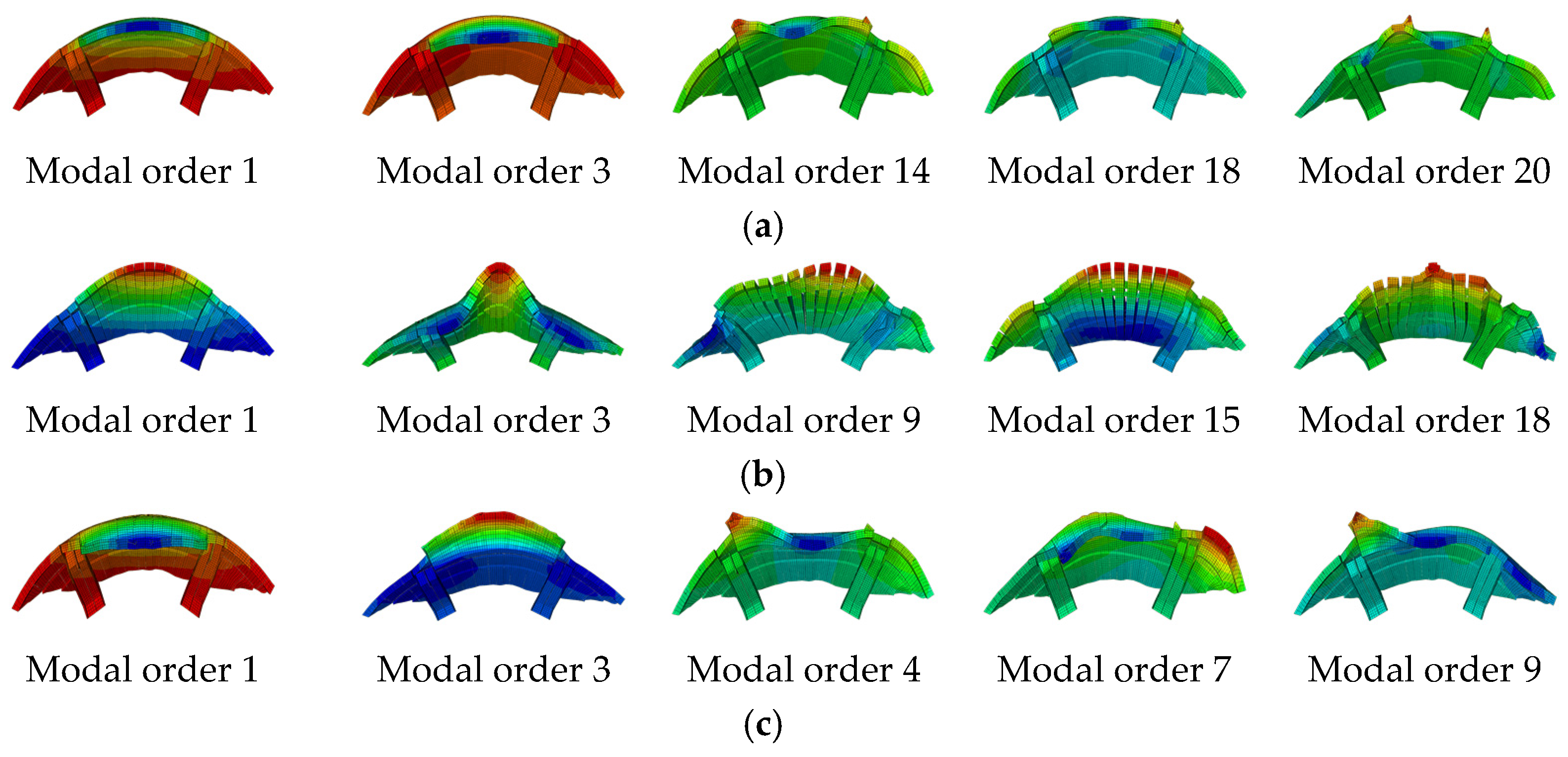
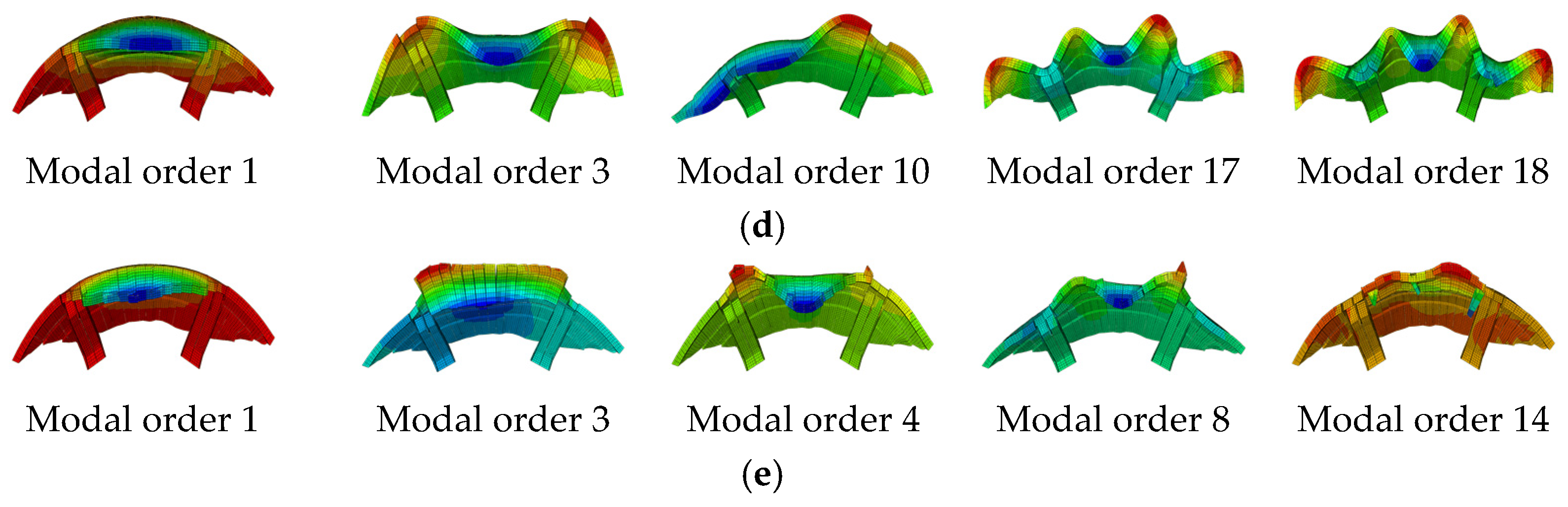
2.3.2. Selection of Target Mode

Many scholars suggest that for some high arch dams, lower modal orders are often considered to have large dynamic response. However, the modal energy is not always concentrated on the low-order modes. For some complex structures, higher modal orders also exhibit large dynamic response [14,23]. Therefore, selecting only the first several modes as the modal shape matrix is not appropriate. To improve the modal energy at sensor locations, this paper employs a modified modal assurance criterion (MMAC) to address this issue. It uses the modal participation factor (MPF) [22] as the criterion for evaluating the dynamic responses of different modes. The new modal shape matrix is then composed of modes with relatively higher modal energy. The MPF is defined as:

$${\phi }_{ir}={\displaystyle \frac{{{\Phi }_i}^{T}M{D}_r}{{{\Phi }_i}^{T}M{\Phi }_i}}$$

(19)

where ${\phi }_{ir}$ is the MPF in r direction for the i-th mode, $\Phi$ is the modal shape matrix, M is the structural mass matrix, and D is a vector that describes the direction of excitation.

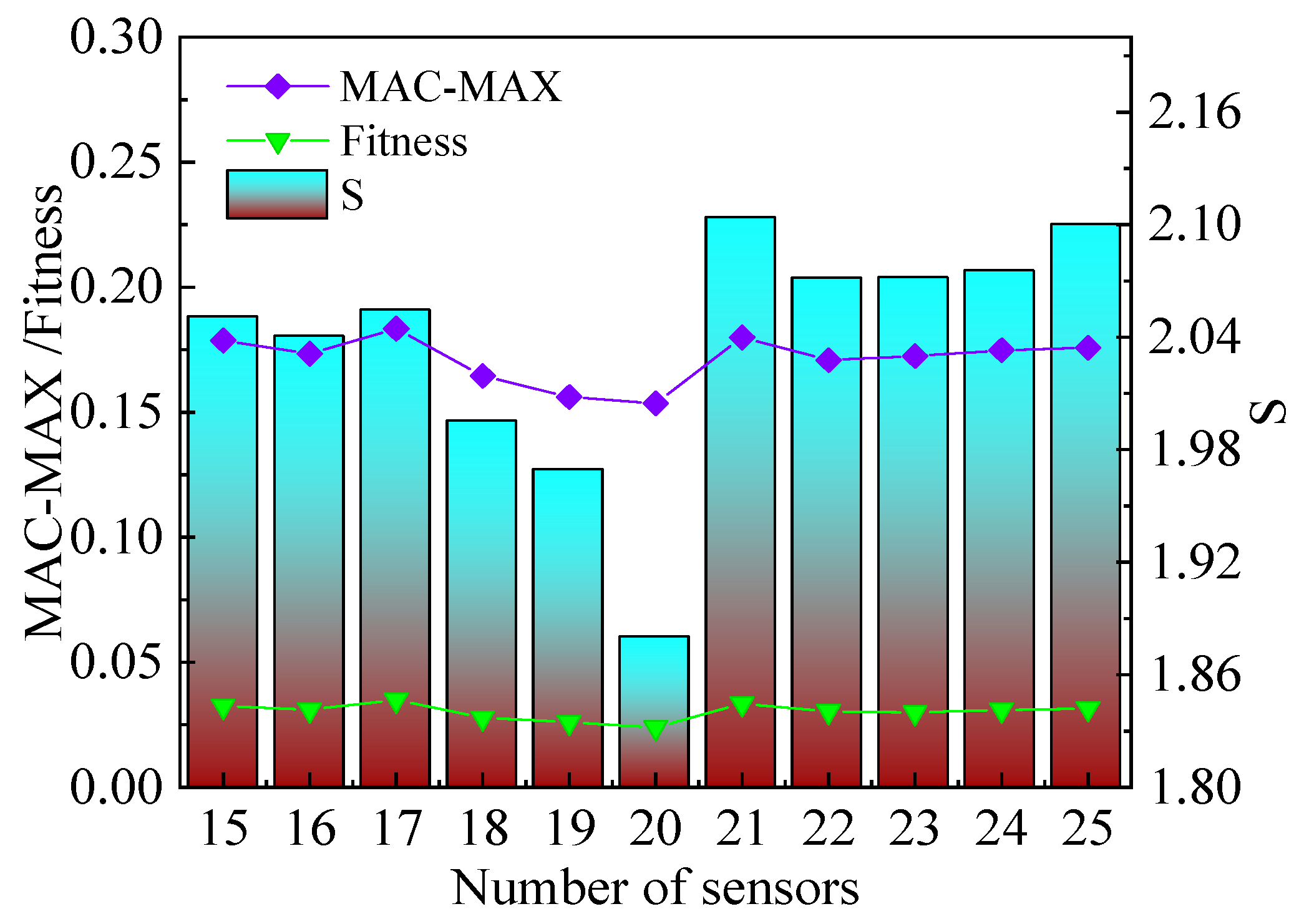
2.3.3. Selection of the Number of Sensors

In this paper, the selection of the number of sensors is carried out by MAC, fitness values, and S criteria [12]. The specific steps are as follows:

(1)

Constructing modal shape matrix $\Phi$ based on target modes and optimized DOFs.

(2)

Conduct QR decomposition on the transpose of the matrix $\Phi$ to determine the initial sensor locations and calculate the corresponding MAC matrix.

(3)

From the remaining DOFs outside the initial sensor locations, select point m to be added to the optimized configuration. Recalculate its MAC matrix, denoted as (MAC_ij)_m, with the maximum off-diagonal element value, denoted as (f_max)_m.

(4)

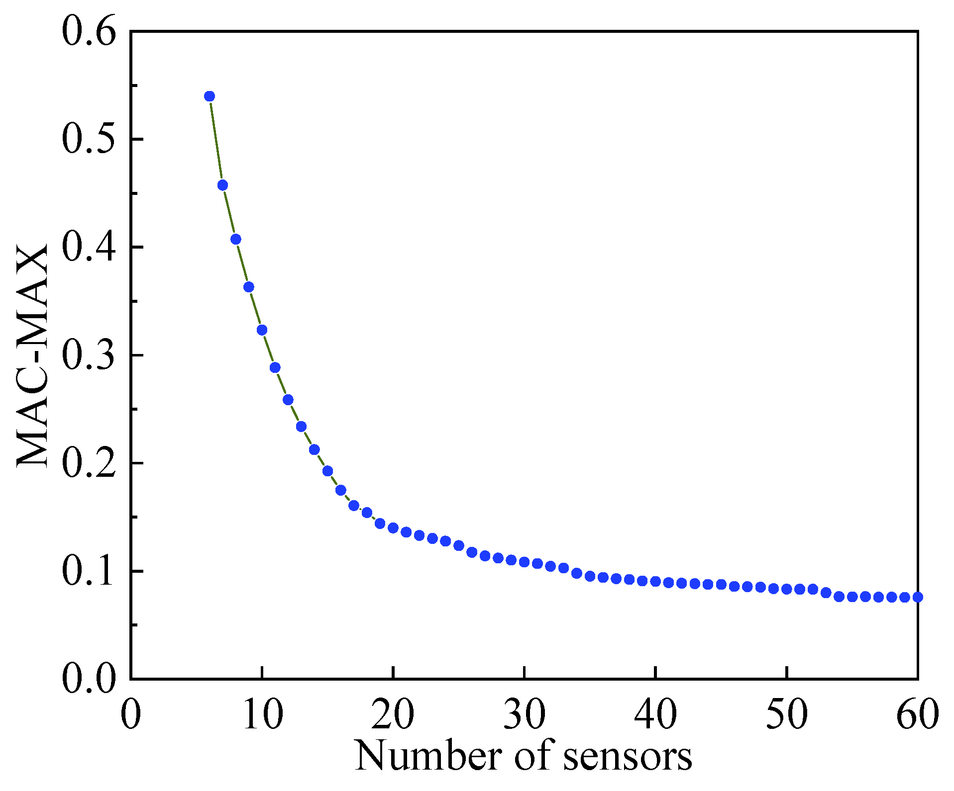
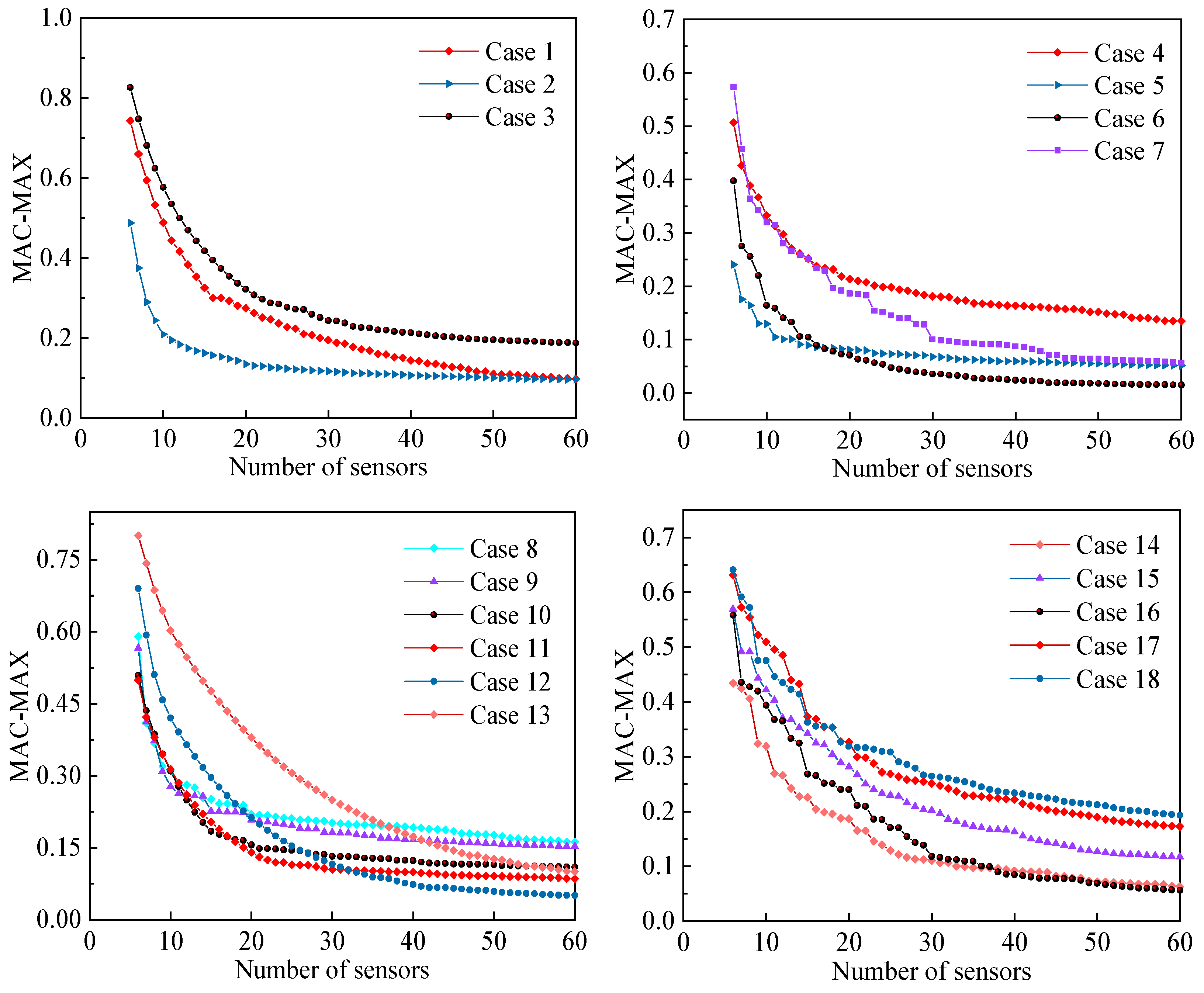
Loop the operation in step (3) to plot the curve of the maximum off-diagonal element value of the MAC matrix with the number of sensors.

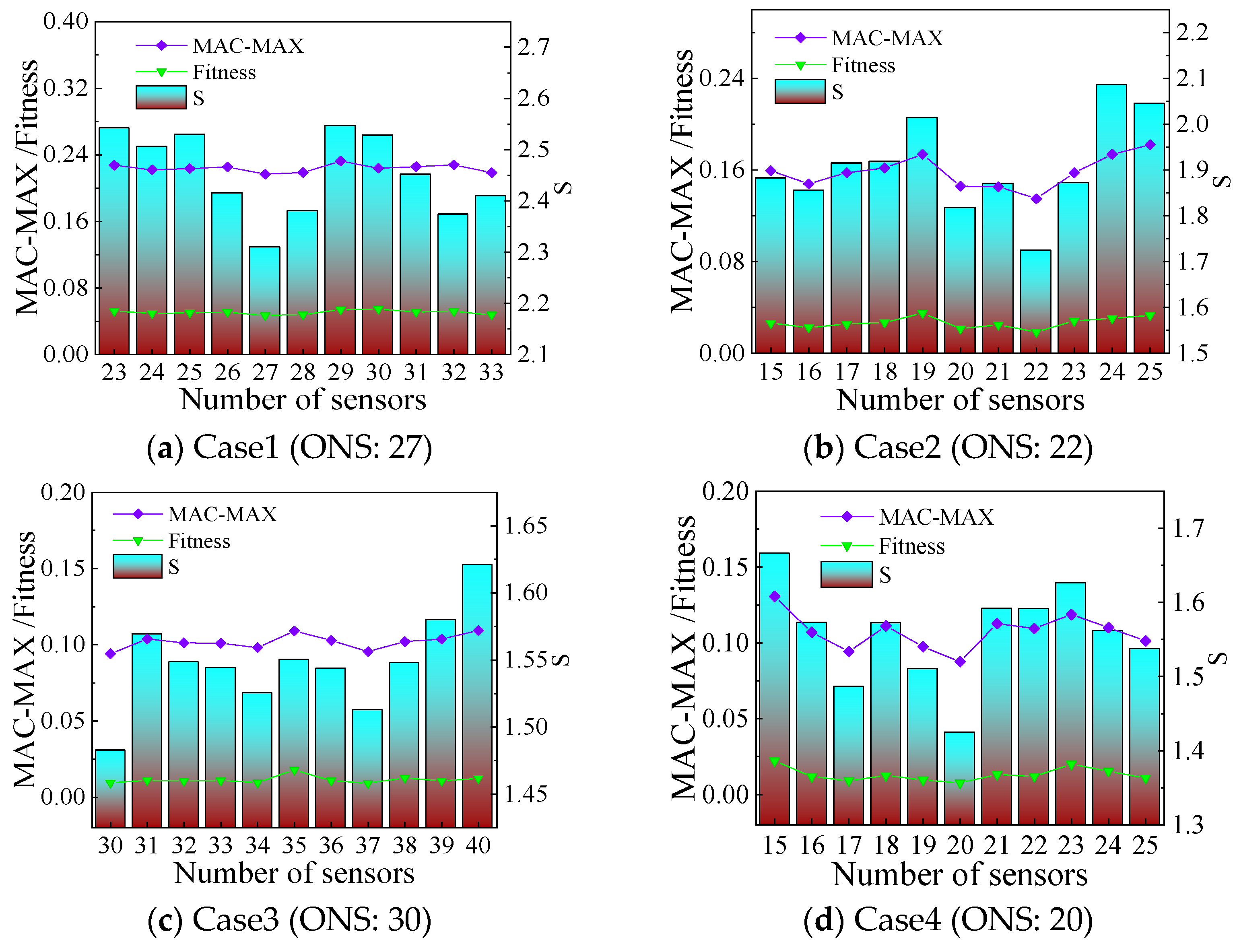
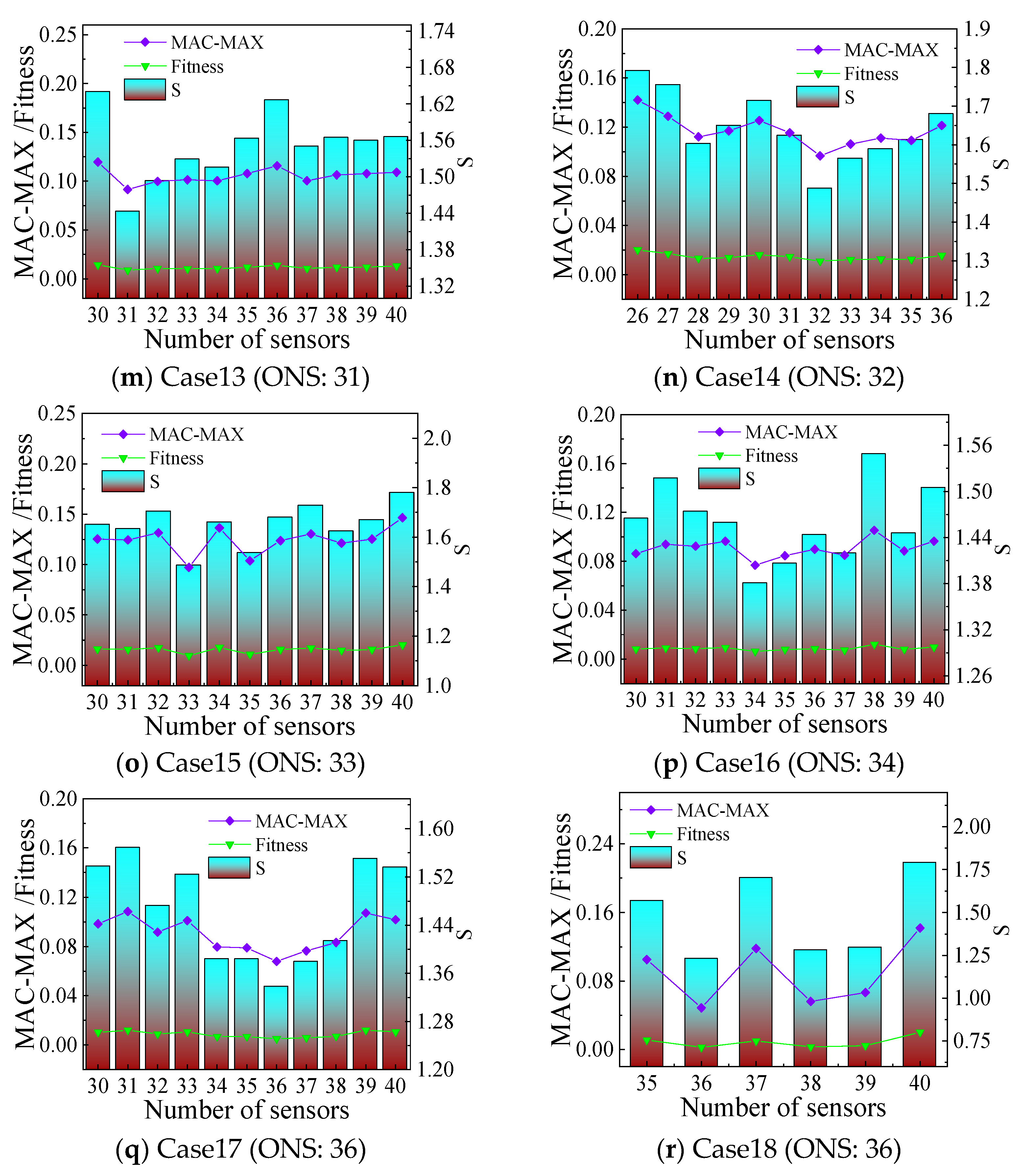
(5)

The appropriate interval segments are selected for the graph in (4) and the ONS is selected using the preferred intelligent algorithm in combination with the maximum value of the off-diagonal elements of the MAC matrix, the value of the function fitness, and the maximum singular value ratio criterion.

Traditionally, most scholars determine the number of sensors based on MAC [12,29] and also use the fitness value [30] to determine the number of sensors. This paper simultaneously considers MAC, fitness value, and S to mutually verify the ONS. These three evaluation indicators all show that the lower the value, the better the sensor layout effect. Therefore, when these three values are calculated multiple times within the selected sensor number interval, the lowest value corresponding to the number of sensors should be the optimal number. The results indicate that the number of sensors determined based on these three criteria is the same for each operating condition, which well verifies the rationality of the optimal sensor number selection method in this paper.

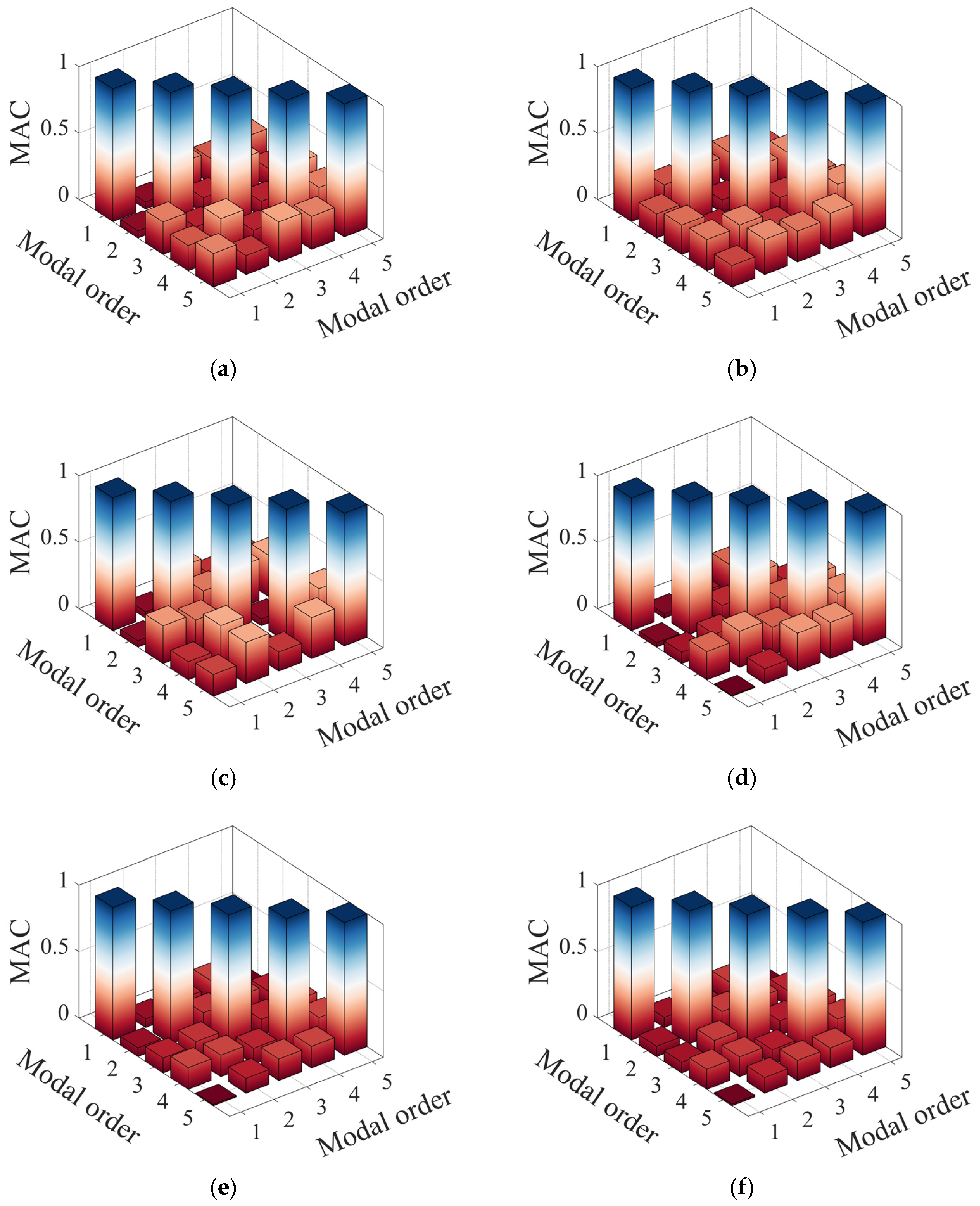
2.3.4. Evaluation Criteria

(1)

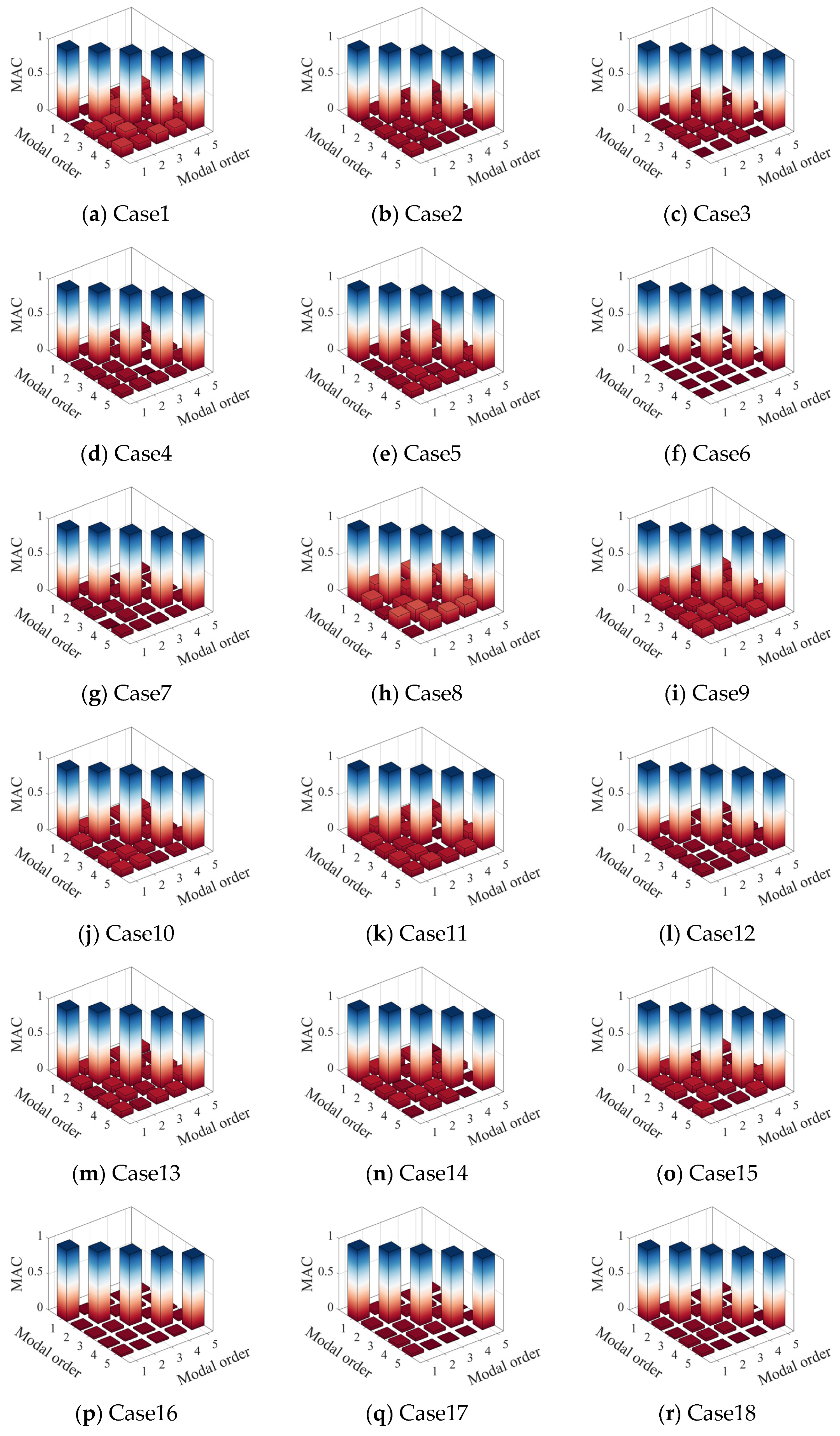
Modal assurance criterion

The modal assurance matrix can effectively evaluate the goodness of orthogonality between the mode shape vectors and is defined as follows [20]:

$$MA{C}_{ij}={\displaystyle \frac{{\left({\Phi }_i^T{\Phi }_j\right)}^2}{\left({\Phi }_i^T{\Phi }_i\right)\left({\Phi }_j^T{\Phi }_j\right)}}$$

(20)

When MAC is 0, it indicates that the i-th and j-th order mode shape vectors have the best orthogonality; when MAC is 1, it indicates that the i-th and j-th order mode shape vectors have the worst orthogonality.

(2)

Singular value ratio criterion

Maximum singular value ratio is an evaluation metric for the singular value decomposition of modal matrices [31]. It can be represented by the following equation:

$$S={\displaystyle \frac{{\sigma }_d}{{\sigma }_m}}$$

(21)

where ${\sigma }_d$ and ${\sigma }_m$ are the maximum and minimum values of the singular values of the modal matrix, respectively. The smaller S is, the better the results obtained.

2.3.5. Fitness Function

The MAC criterion can evaluate the OSP problem well because the maximum value of the off-diagonal elements of the MAC matrix (MAC-MAX) of the two modal vectors is 1, and the MAC method generally minimizes the off-diagonal elements, so for the convenience of calculation, the fitness function constructed in this paper is as follows:

$$f(x)=\max \left\{MA{C}_{ij}\right\}\hspace{1em}(i\ne j)$$

(22)

where the closer the function $f\left(x\right)$ is to 0, the better the scheme is.

2.4. OSP Framework of Arch Dams with Cracks Based on IAHA

This section mainly introduces the OSP framework for arch dams with cracks based on IAHA. Figure 2 shows the flow chart of the framework, and the specific implementation process is as follows:

Step 1: According to the engineering data, the appropriate modeling range and element size are selected to establish the arch-dam–reservoir–foundation 3D finite element model. The reservoir water element is simulated by acoustic element. According to Equations (9)–(12), contraction joints are simulated by contact model. According to Equations (7) and (8), cracks are simulated by cohesive element.

Step 2: Considering the role of dynamic water pressure, Equations (1)–(6) are used to analyze the dynamic characteristics of this arch dam, comparing the results of the Westergaard added mass model and FSCM and arguing for the reasonableness and accuracy of FSCM in simulating the dynamic water pressure.

Step 3: The MPF is calculated according to Equation (19), and the MMAC is chosen to combine the MPF to select the modal orders with relatively high modal energies and form a new modal shape matrix.

Step 4: According to Equations (14)–(18), an improved circle chaotic mapping and Levy flight are introduced to optimize the artificial hummingbird algorithm, and the optimized algorithm is named IAHA, where the objective function of the intelligent algorithm is shown in Equation (22).

Step 5: Combined with the traditional method to select the number of sensors initially, under the premise of the same number of sensors, intelligent algorithms are used to carry out the OSP for the arch dam. Comparison and analysis of the performance of each algorithm and the effect of sensor placement verify and analyze that IAHA is the most suitable intelligent algorithm for the fitness function in this paper.

Step 6: Based on the preferred IAHA, combined with the method outlined in Section 2.3.3, the ONS under the corresponding working condition is re-selected by MAC, fitness values, and S criteria. According to Equations (20) and (21), compare the outcomes with the initial selections to validate the rationality and feasibility of the sensor quantity selection method proposed in this paper.

Step 7: Adopting the above method, this paper analyzes the effects of the evolution of structural states and material properties of a dam body on the quantity and spatial location of sensors for the arch dam and investigate the change rule of the sensor placement results. This mainly includes the following cases: (1) considering only the case of horizontal cracks or vertical cracks or their superposition; (2) considering only the existence of contraction joints and elastic modulus degradation of contraction joints; (3) considering only the case of the zoning of dam body; (4) considering only the case of elastic modulus zoning degradation of dam body; (5) comprehensive consideration of the presence of cracks, contraction joints, and elastic modulus zoning degradation of a dam body.

Step 8: Finally, after 45 years of operation, sensors are placed for the current state of the arch dam, and the ONS is selected, along with the final spatial location results of the sensors.

3. Case Study

3.1. Model Information

For a certain arch dam, the maximum dam height is 76.30 m, the crest elevation is 126.30 m, the arc length of the crest is 419.00 m, the thickness of the crest is 8.00 m, the thickness of the bottom is 53.25 m, and the normal storage level of the reservoir is 119.00 m [55]. After finite element model calculation, it is recommended to select the appropriate range of foundation modeling for this arch dam, which is three times the dam height along the depth direction of the foundation, the length direction of the left and right banks, and the upstream and downstream length direction. For the calculation and analysis in this paper, it is assumed that the dam concrete and the foundation are isotropic linear elastic materials, in which the modulus of elasticity of the dam concrete is 24.75 GPa, the Poisson’s ratio is 0.2, and the density is 2450 kg/m³. The elastic modulus of foundation material is 15 GPa, Poisson’s ratio is taken as 0.2, and the density is taken as 1 × 10⁻⁶ kg/m³. The two methods of the Westergaard added mass model and FSCM are adopted to simulate the reservoir dynamic hydraulic pressure, where the reservoir density is taken as 1000 kg/m³, the bulk modulus of the reservoir water is taken as 2.07 × 10⁹ Pa when the compressibility of the reservoir water is considered, and the bulk modulus of the reservoir water is taken as 2.07 × 10²⁰ Pa when the compressibility of the reservoir water is not considered. The construction of this dam spanned three phases. Phase I involved concrete pouring from 1959 to 1962. Phase II was completed in 1969–1972 and poured to the original design elevation of 125.00 m. The phase III of concrete pouring was completed in 1978 and poured to the current elevation of 126.30 m [56]. Therefore, it is necessary to consider the impact of dam material zoning on OSP. This paper divides the dam body into three regions based on the actual project, the specific zoning situation is shown in Figure 3. The initial elastic modulus of the concrete arch dam is 16.5 GPa, and the corresponding dynamic elastic modulus is taken as 1.5 times the static elastic modulus. By 2023, the dam has been in operation for 45 years. According to Equation (13), the degradation of elastic modulus in various regions of dam body is presented in

Table 1. Statistical table of elastic modulus degradation in various regions of the arch dam after 45 years of operation.

Element	Material Parameters	Years of Degradation	Phase I (GPa)	Phase II (GPa)	Phase III (GPa)
Dam	Elastic modulus	0	24.27	24.84	24.75
Dam	Elastic modulus	10	22.92	24.27	24.72
Dam	Elastic modulus	20	20.97	22.92	23.81
Dam	Elastic modulus	30	18.56	20.97	22.20
Dam	Elastic modulus	40	15.84	18.56	20.04
Dam	Elastic modulus	45	14.43	17.22	18.81

.

During the construction of this arch dam, insufficient attention was given to temperature control measures, resulting in the generation of numerous cracks in the dam body. Some of these cracks have posed a significant threat to the dam’s safety. The main severe cracks include the following: (1) horizontal cracks near elevations of 105 m and 111.5 m in the downstream surface, penetrating through 24 and 16 dam sections, with depths reaching 6 m and 12 m, respectively; (2) longitudinal vertical cracks on the dam crest, with depths exceeding 8 m [57]. The schematic distribution of these horizontal and longitudinal vertical cracks is illustrated in Figure 3. Additionally, based on measured data, there are numerous vertical cracks on the upstream surface of the dam.

Table 2. Statistical table of vertical cracks on the upstream surface of the arch dam.

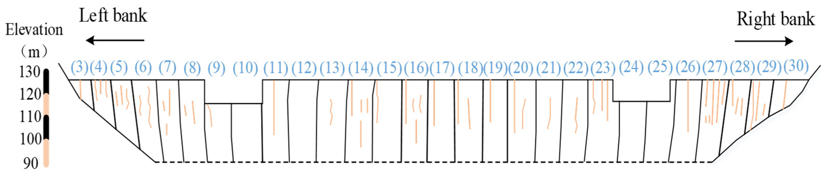
Dam Sections	3	4	5	6	7	8	9	10	11	12
Crack number	1	3	3	2	3	2	1	-	1	-
Crack length (m)	8	9~10	2.5~6	3~13	2~3.5	2~6	10	-	20	-
Crack width (mm)	-	-	0.2	0.2	-	0.3	-	-	-	-
Dam sections	13	14	15	16	17	18	19	20	21	22
Crack number	1	4	1	4	1	2	1	2	1	1
Crack length (m)	4	2.5~10	11	2~14	11	10~15	12	10~20	9	9
Crack width (mm)	0.5	-	-	-	-	-	-	-	-	0.5
Dam sections	23	24	25	26	27	28	29	30
Crack number	3	-	-	1	6	3	3	1
Crack length (m)	12~15	-	-	21	1.5~21	10~12	2~29	9
Crack width (mm)	-	-	-	0.3	0.3	0.3	-	-

and Figure 4 provide specific details about their distribution [58]. In this paper, two horizontal cracks near elevations of 105 m and 111.5 m in the downstream surface, some longitudinal vertical cracks on the dam crest, and representative vertical cracks are selected for analysis. The selected representative vertical cracks are all over 13 m in length, located in dam sections 6, 11, 16, 18, 20, 23, 26, 27, and 29, totaling nine vertical cracks.

Figure 5a shows an on-site image of the arch dam. As illustrated in Figure 5b–d, the coordinate system of the dam model is defined with the dam axis direction as the x-axis, pointing toward the left bank as positive, along the river flow direction as the y-axis, pointing toward the upstream as positive, and the vertical direction as the z-axis, with positive direction pointing vertically upward. Figure 5b–d show the mesh of the dam body, foundation, and reservoir water, while Figure 5e displays the situation of contraction joints, and Figure 5f presents the mesh of crack elements. The calculations are conducted using ABAQUS. The entire dam body consists of 42,140 C3D8 elements, the foundation comprises 66,859 C3D8 elements, and the reservoir water consists of 49,875 AC3D8 elements. There are 692 COH3D8 elements for horizontal cracks and 469 COH3D8 elements for vertical cracks. The simulation methods in Section 2.2 are employed for cracks and contraction joints. The tensile strength of crack elements is set to 0.6 MPa [59]. The mesh size and element types have been calculated and calibrated for dynamic characteristics in the previous work, and the stress, displacement, and frequency calculated by the model are relatively stable. The specific process can be found in reference [60].

3.2. Model Analysis

The prerequisite for the OSP of arch dams is to conduct a natural frequency analysis, and the influence of reservoir water on natural frequencies cannot be ignored. Many scholars have employed the added mass method proposed by Westergaard to simulate the effect of reservoir water on the upstream surface of a dam body. However, this method neglects the compressibility of the reservoir water, leading to an overestimation of the calculated natural frequencies. To simulate the dynamic characteristics of the dam more realistically, two methods, Westergaard added mass model and FSCM, are used to simulate the dynamic water pressure of the reservoir water, which is divided into four models for discussion, namely, an empty reservoir model I without considering the reservoir water, an Westergaard added mass model II with a reduction factor of 0.5, an incompressible fluid solid coupling model III, and a compressible fluid solid coupling model IV. Because the optimal sensor placement is based on the modal information calculated through dynamic characteristic analysis of the model, and the model established based on FSCM is more reasonable, the results of sensor optimization arrangement are also more reasonable. Calculated natural frequencies and mode shapes are presented in

Table 3. Different natural frequencies of the arch dam under different reservoir water models (Hz) (water level 119 m).

Modal Order	I	II	III	IV	Modal Order	I	II	III	IV
1	3.4447	3.1309	3.0199	2.9709	11	9.3860	8.9263	7.9325	6.6295
2	4.0645	3.8043	3.6285	3.5753	12	9.5225	8.9739	8.2783	6.9863
3	5.1442	4.8549	4.6347	4.3085	13	9.7931	9.1956	9.0917	7.4745
4	5.9358	5.6521	5.6255	4.5607	14	10.448	10.102	9.1782	7.5211
5	6.1389	5.7804	5.8691	5.2231	15	10.847	10.252	9.2030	7.5768
6	6.7329	6.5518	5.8905	5.3010	16	11.251	10.794	9.5273	7.8364
7	7.1386	6.7042	6.6500	5.5621	17	12.170	11.418	10.063	8.0440
8	8.1281	7.5553	6.7196	5.8306	18	12.233	11.460	10.385	8.5419
9	8.3435	7.9089	7.6961	6.2930	19	12.726	12.194	10.762	8.6655
10	8.4638	8.1444	7.7990	6.5597	20	13.198	12.584	10.816	8.6964

and Figure 6. Table 3 presents the natural frequencies of the first 20 modal orders calculated, while Figure 6 shows the first 5 modal orders. Modal order refers to the number of eigenvalues obtained by a structure in modal analysis. In finite element analysis, the essence of modal analysis is to find the eigenvalues of a matrix, and the number of eigenvalues is the order of the modal. Due to the infinite dimensionality of the actual analysis object, its modals have infinite orders, but in calculations, only the first few modal orders are usually considered. This article focuses on the first 20 modal orders.

According to Table 3, natural frequencies of models II, III, and IV are lower compared to model I. This indicates that the presence of reservoir water causes a decrease in the natural frequencies of the arch dam. This is consistent with the principle that, when considering reservoir water, the system’s mass increases while the stiffness remains constant, leading to a reduction in natural frequencies [39]. Model IV has the lowest natural frequency, suggesting that considering the compressibility of reservoir water has the most significant impact on natural frequencies of the arch dam. Based on Figure 6, it is evident that the modal shapes vary when considering the compressibility of reservoir water, compared to the other three models. Taking the fourth modal shape as an example, model IV exhibits a symmetric modal shape, while the other three models display anti-symmetric shapes. This indicates that considering the compressibility of reservoir water has a certain effect on the modal shapes of the arch dam. In summary, when conducting natural frequency analysis for the arch dam, it is essential to consider the influence of the compressibility of reservoir water. As is well known, the application of the FSCM in various hydraulic structures has been mature. Many scholars, such as reference [61], have demonstrated that using FSCM is more accurate than using the Westergaard added mass model on dams. At the same time, the dynamic characteristics calculated based on the FSCM in this paper are consistent with the conclusions of references [39,62].

3.3. OSP in Seamless Condition

3.3.1. Selection of Target Mode

For large hydraulic structures like arch dams, under the excitation of dynamic water pressure, the vibration is mainly along the river flow direction (y-direction). Without loss of generality, this paper focuses on the OSP of the downstream surface of the arch dam along the river flow direction [31]. MPF reflects the dynamic response amplitudes of all modes. When constructing a new modal shape matrix, it is advisable to prioritize the selection of modes with larger MPF. Traditionally, the first five modes of arch dams are commonly chosen as target modes [63]. In this section, based on the consideration of MPF, the first five modes with higher modal energy are selected to form a new modal shape matrix. This approach aims to obtain higher modal information by selecting a fewer number of modes whenever possible. As shown in Figure 7, the 1st, 4th, 10th, 15th, and 17th modal orders of the arch dam exhibit significant MPF along the river flow direction. Therefore, these five modal orders are selected as the latest modal shape matrix. The corresponding mode shapes are illustrated in Figure 8.

3.3.2. Select the Number of Sensors

Once the target number of modes is determined, the next step is to determine the number of sensors. The vibration response of measuring points near the top of the arch dam is relatively large, which is conducive to the identification of modal parameters, and sensors generally cannot be placed underwater [30]. To avoid excessive concentration of sensors and unnecessary information redundancy, 188 initial candidate measurement points are selected at equal intervals on the downstream surface of the arch dam, as shown in Figure 9. According to selected modal orders, the curve of MAC-MAX versus the number of sensors is plotted, as shown in Figure 10.

When MAC-MAX is less than 0.25, it can be considered that modal shape vectors can be well distinguished. The preliminary principles for selecting the number of sensors in this paper are as follows: (1) MAC-MAX should be less than or equal to 0.25; (2) try to choose the stable phase of curve descent as much as possible; (3) considering the economic requirements, the number of sensors should not be too high, and this paper stipulates that the number of sensors should not be more than 40, which is consistent with the number of sensors in references [7,31,33]. According to Figure 10, as the number of sensors increases, the curve undergoes the most significant changes between 0 and 20 sensors. After placing 20 sensors, the MAC-MAX curve gradually stabilizes, ranging from 0.0758 to 0.1398, with a small variation. Further increasing the number of sensors contributes little to the reduction in MAC-MAX. Therefore, this section recommends selecting 20 sensors for placement.

3.3.3. Optimal Sensor Placement

In this section, comparison and optimization are performed using six intelligent algorithms, including PSO, IPSO, SSA, ISSAMS, AHA, refs. [49,50,52,53,54], and IAHA. Considering the stochastic nature of intelligent algorithms, each algorithm is run 10 times, and the optimal value is selected. The sensor placement results are illustrated in Figure 11, where sensors are indicated by red dots in Figure 11. From Figure 11, It can be clearly judged from the spatial layout that the sensor layout placed using intelligent algorithms is relatively scattered. This suggests that introducing intelligent algorithms for sensor placement can effectively reduce the issue of sensor concentration, thus avoiding significant redundancy in modal information. Additionally, most sensors are concentrated in the upper-middle part of the downstream surface of the dam, which is consistent with the characteristic that the vibration mode information of arch dams is mainly concentrated in the upper-middle part of the dam body. The sensor placements obtained from the above results are consistent with the results in references [7,30,32], verifying the rationality and effectiveness of the method.

3.3.4. Evaluation of OSP Results

To further analyze the differences between various intelligent algorithms, quantitative analysis is conducted using MAC, fitness values, and S criteria to determine the most suitable optimization algorithm for this arch dam [20,31]. To describe the modal independence of solutions obtained by different algorithms, the maximum value of the off-diagonal elements of the MAC matrix (MAC-MAX), the average value of the off-diagonal elements of the MAC matrix (MAC-AVE), the root mean square of the off-diagonal elements of the MAC matrix (MAC-RMS), and the maximum singular value ratio (S) are chosen as evaluation criteria, and the smaller the value of these four indexes, the better the results of sensor placement. The evaluation metrics and MAC matrix diagrams of the layout results of different optimization methods are shown in Figure 12 and Figure 13.

From Figure 12 and Figure 13, it is apparent that the results of sensor placement obtained by all improved intelligent algorithms are superior to the results before improvement. The four indicators of IAHA are all smaller than the other five intelligent algorithms, among which MAC-MAX has decreased by 50%, 45%, 53%, 47%, and 8% compared to the other five intelligent algorithms, respectively; MAC-AVE has reduced by 50%, 50%, 47%, 33%, and 11% compared to the other five intelligent algorithms, respectively; MAC-RMS has reduced by 45%, 42%, 44%, 34%, and 5% compared to the other five intelligent algorithms, respectively; S has reduced by 38%, 33%, 43%, 34%, and 7% compared to the other five intelligent algorithms, respectively. Among the six intelligent algorithms, IAHA shows the best performance, with its four indicators being smaller than the other five intelligent algorithms. Therefore, IAHA demonstrates the most effective optimization for the fitness function used in this paper.

To validate the superiority of IAHA, a further analysis of six intelligent algorithms is conducted in terms of algorithm performance. Since the performance and solution outcomes of intelligent algorithms are significantly influenced by the initialization parameters of the program, efforts are made to align these six algorithms on a similar starting line as much as possible before testing and set the population size of each algorithm to 100, the number of iterations to 500, and the variable dimension to 20. The remaining parameter settings for each algorithm are shown in

Table 4. Parameter settings for various intelligent algorithms.

Algorithm Name	Inertia Weight	Acceleration Coefficients	Maximum Velocity	Safety Threshold	Producers’ Number
PSO	w = 0.9	2	20	-	-
IPSO	wmax = 0.9, wmin = 0.4	2	20	-	-
SSA	-	-	-	0.6	0.8
ISSAMS	-	-	-	0.6	0.8
AHA	-	-	-	-	-
IAHA	-	-	-	-	-

. Due to the inherent stochastic nature of intelligent algorithms, this paper runs 10 times on each of the six algorithms. The maximum, average, and minimum fitness values of each algorithm are compared, and the corresponding convergence curves are plotted in Figure 14.

According to Figure 14, in terms of algorithm convergence accuracy, the convergence curves of the maximum, average, and minimum fitness values for the improved algorithms in the 10 runs all show better performance, and IAHA has the best convergence performance. According to Table 4, in terms of algorithm parameter settings, AHA and IAHA only need to set three parameters, while PSO, IPSO and SSA, ISSAMS need to set six and five parameters, respectively. From the convergence time of the algorithms, according to

Table 5. Average running time of each algorithm.

Algorithm Name	PSO	IPSO	SSA	ISSAMS	AHA	IAHA
Run time/s	202.15	202.60	99.99	106.07	101.32	101.43

, it can be seen that the respective algorithms have increased in time compared to the time before the improvement; this is because the improved algorithms do not change the principle of the algorithm itself but only initialize the respective algorithms to initialize the populations more adequately or introduce a mathematical model describing the stochastic motion in the middle of the algorithms, which inevitably increases the algorithms’ time in terms of the principle but tend to bring about a higher degree of accuracy; IAHA is not inferior to ISSAMS in terms of time cost, and IAHA takes the least time among the three improved intelligent optimization algorithms, only 101.43 s, which also shows the superiority of IAHA. Therefore, IAHA is the most advantageous algorithm. In summary, combining the evaluation indexes of the intelligent algorithm placement results, the MAC matrix diagram, and the convergence stability of the algorithm and other factors, the most suitable intelligent algorithm for the OSP of the model in this paper is IAHA, which will be used for the relevant computational analyses in a later paper.

In the past, the number of sensors was selected based on observing the curve of MAC-MAX with the number of sensors and combining the economic conditions and other factors, which may not be the optimal solution. In order to have a clear judgement criterion for the determination of the number of sensors, combined with the principle of the preliminary selection of the number of sensors in the previous section, the interval of the number of sensors is selected to be [15,25], and then the IAHA is used to calculate the fitness value, MAC-MAX, and S in this interval, and the curve and bar graph are plotted to determine the ONS, where each calculation is run 10 times to take the average value; the calculation results are shown in Figure 15. According to Figure 15, the number of sensors corresponding to the minimum MAC-MAX and fitness value is 20, and the number of sensors preferred by the S criterion is also 20. Therefore, 20 sensors can be selected to achieve the optimal layout effect, which indicates that it is feasible to achieve the ONS by the judgement criterion. The number of sensors selected by this judgement criterion is also consistent with the number of sensors initially selected in Section 3.3.2.

3.4. OSP Considering the Evolution of Structural States and Material Properties

Arch dams are subjected to long-term loads and environmental effects during operation, which lead to the evolution of structural states and material properties, including the degradation of contraction joints, the appearance of cracks, and elastic modulus zoning degradation of the dam body. The evolution of structural states and material properties in an arch dam can reduce the dam’s stiffness, resulting in a decrease in the system’s natural frequencies and subsequently affecting the placement of sensors. To investigate the impact of factors such as cracks, contraction joints, and elastic modulus zoning degradation of the dam body on the placement of sensors on the downstream surface of the arch dam, 18 different cases are set up for calculation and analysis. The specific settings for the 18 cases are provided in

Table 6. Setup of cases considering the evolution of structural states and material properties.

Case	Cracks, Contraction Joints, and Elastic Modulus Degradation	Schematic Diagram of Cracks	Case	Cracks, Contraction Joints, and Elastic Modulus Degradation	Schematic Diagram of Cracks
1	Horizontal cracks		10	Dam’s elastic modulus zoning degradation for 20 years	-
2	Vertical cracks		11	Dam’s elastic modulus zoning degradation for 30 years	-
3	Horizontal and Vertical cracks		12	Dam’s elastic modulus zoning degradation for 40 years	-
4	Contraction joints 0.25 GPa		13	Dam’s elastic modulus zoning degradation for 45 years
5	Contraction joints 2 GPa		14	Dam’s elastic modulus zoning degradation for 10 years with all cracks
6	Contraction joints 10 GPa		15	Dam’s elastic modulus zoning degradation for 20 years with all cracks
7	Contraction joints and cracks		16	Dam’s elastic modulus zoning degradation for 30 years with all cracks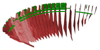
8	Dam material zoning	-	17	Dam’s elastic modulus zoning degradation for 40 years with all cracks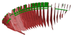
9	Dam’s elastic modulus zoning degradation for 10 years	-	18	Dam’s elastic modulus zoning degradation for 45 years with all cracks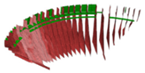

Notes: (1) vertical cracks in the table include selected longitudinal vertical cracks on the dam crest and vertical cracks on the upstream surface of the dam; (2) the modulus of elasticity of the contraction joints in case 7 and cases 14~18 is set to 0.25 GPa.

.

The contact elastic modulus of contraction joints significantly influences the natural frequencies of arch dams [42]. To study the effect of different elastic moduli of contraction joints on OSP, the elastic moduli of the contraction joints are taken as k = 0.25 GPa, 0.5 GPa, 1 GPa, 2 GPa, 10 GPa, and 20 GPa. Figure 16 shows the first-order natural frequency curves for different elastic moduli of contraction joints. As the elastic modulus of the contraction joint increase, the natural frequency of the arch dam significantly increases. The most noticeable change in natural frequencies occurs in the range of about 0.25 to 2 GPa, becomes gradual in the range of about 2 to 10 GPa, and stabilizes in the range of about 10 to 20 GPa, consistent with reference [42]. If the elastic modulus of contraction joints degrades over 45 years, as according to Equation (13), its elastic modulus only degrades to about 12.5 GPa, and the corresponding dynamic elastic modulus is about 18.8 GPa. It has a minimal impact on the natural frequencies of the arch dam, as is evident from Figure 16. To study the influence of contraction joints on sensor layout, this paper selects the elastic modulus values with the more obvious curve changes in Figure 16, which are 0.25 GPa, 2 GPa, and 10 GPa, respectively.

To assess the impact of the elastic modulus of horizontal and vertical cracks on the natural frequencies of the arch dam, crack elastic modulus values are chosen to be approximately 10-1, 10-2, and 10-3 times the dam body elastic modulus, with values of 2 GPa, 0.2 GPa, and 0.02 GPa, respectively. The results are presented in

Table 7. Natural frequencies of horizontal and vertical cracks under different elastic moduli.

Modal Order	Cracks (0.02 GPa)	Cracks (0.2 GPa)	Cracks (2 GPa)	Modal Order	Cracks (0.02 GPa)	Cracks (0.2 GPa)	Cracks (2 GPa)
1	2.8891	2.8895	2.8929	11	5.8649	5.8669	5.8860
2	3.4420	3.4425	3.4473	12	6.3409	6.3415	6.3477
3	4.1633	4.1689	4.2144	13	6.5978	6.5979	6.5984
4	4.3398	4.3408	4.3510	14	6.7701	6.7715	6.7855
5	4.4205	4.4232	4.4575	15	6.9667	6.9683	6.9823
6	4.8874	4.8911	4.9256	16	7.0870	7.0881	7.0988
7	5.2322	5.2325	5.2350	17	7.5251	7.5254	7.5286
8	5.2917	5.2917	5.2920	18	7.6363	7.6370	7.6436
9	5.5773	5.5797	5.6046	19	7.8475	7.8479	7.8517
10	5.8059	5.8059	5.8064	20	8.2465	8.2483	8.2649

. From Table 7, it is evident that natural frequencies of the arch dam change very little for the three chosen crack elastic modulus values. This indicates that the variation in crack elastic modulus has a very small effect on the natural frequencies of the dam body and can be neglected. Therefore, in the calculations and analysis of this paper, the crack elastic modulus is set to 0.02 GPa.

3.4.1. Selection of Target Mode

Calculate the normalized MPF for the 18 cases considering the cracks, contraction joints, and elastic modulus zoning degradation of the dam body, as shown in Figure 17. Select the modal orders corresponding to higher modal energy, as presented in

Table 8. Modal orders selected for 18 cases.

Case	Selected Modal Orders	Case	Selected Modal Orders	Case	Selected Modal Orders
Case 1	Order: 1, 2, 6, 18, 20	Case 7	Order: 1, 3, 4, 7, 9	Case 13	Order: 1, 3, 10, 17, 18
Case 2	Order: 1, 4, 10, 15, 17	Case 8	Order: 1, 4, 10, 15, 17	Case 14	Order: 1, 3, 4, 7, 9
Case 3	Order: 1, 3, 14, 18, 20	Case 9	Order: 1, 4, 10, 15, 17	Case 15	Order: 1, 3, 4, 6, 9
Case 4	Order: 1, 3, 9, 15, 18	Case 10	Order: 1, 4, 11, 15, 17	Case 16	Order: 1, 3, 4, 9, 12
Case 5	Order: 1, 3, 9, 17, 18	Case 11	Order: 1, 4, 9, 16, 17	Case 17	Order: 1, 3, 4, 8, 14
Case 6	Order: 1, 4, 10, 15, 17	Case 12	Order: 1, 3, 10, 17, 18	Case 18	Order: 1, 3, 4, 8, 14

. Due to space limitation, representative mode shapes for selected cases are illustrated in Figure 18.

3.4.2. Select the Number of Sensors

Based on the selected modal orders for 18 cases, the corresponding MAC-MAX versus the number of sensors is plotted, and the results are shown in Figure 19.

To determine the optimal number of sensors (ONS), considering the preliminary selection principles for the number of sensors in previous sections, the initially selected sensor quantity ranges for 18 cases are shown in

Table 9. Preliminary selection of sensor quantity range for 18 cases.

Case	Number of Sensors When MAC ≤ 0.25	MAC Curve Smooth Inflection Point	Selected Interval	Case	Number of Sensors When MAC ≤ 0.25	MAC Curve Smooth Inflection Point	Selected Interval
Case 1	23	28	23~33	Case 10	12	20	15~25
Case 2	9	20	15~25	Case 11	13	22	17~27
Case 3	30	30	30~40	Case 12	18	30	25~35
Case 4	15	20	15~25	Case 13	30	40	30~40
Case 5	6	20	15~25	Case 14	13	26	26~36
Case 6	8	20	15~25	Case 15	22	40	30~40
Case 7	16	30	25~35	Case 16	19	30	30~40
Case 8	15	20	15~25	Case 17	30	40	30~40
Case 9	15	20	15~25	Case 18	35	30	35~40

. Use IAHA to calculate the MAC-MAX, fitness value, and S for all ranges, and plot the curves and histograms as shown in Figure 20. Each calculation is performed 10 times, and the average values are taken. From Figure 20, it can be observed that the number of sensors corresponding to the minimum MAC-MAX and minimum fitness value for each case are as follows: 27, 22, 30, 20, 20, 20, 32, 20, 20, 22, 24, 29, 31, 32, 33, 34, 36, and 36. The number of sensors selected through the S criterion is 27, 22, 30, 20, 20, 20, 32, 20, 20, 22, 24, 29, 31, 32, 33, 34, 36, and 36, respectively, which is consistent with the results selected by MAC-MAX and fitness value. This indicates that the selected numbers for each case can achieve the optimal placement. This also demonstrates that the method proposed in this paper, based on both MAC, fitness values, and S criteria for selecting the ONS, is feasible.

Figure 20 shows that the selected number of sensors for 18 cases are 27, 22, 30, 20, 20, 20, 32, 20, 20, 22, 24, 29, 31, 32, 33, 34, 36, and 36, respectively. In most cases, the number of sensors has increased compared to the seamless condition, with only no changes when considering contraction joints, dam material zoning, and the dam’s elastic modulus zoning degradation for 10 years, separately. In terms of the number of sensors, the influence of cracks is greater than that of contraction joints, especially when affected by two long-distance horizontal cracks at elevations of 105 m and 111.5 m in the downstream surface. Considering the elastic modulus zoning degradation of the dam body, as the degradation period increases, the number of sensors also increases.

3.4.3. Optimal Sensor Placement

Based on the optimal selection of modal orders and sensor quantity, the sensor placement for this arch dam is optimized. The sensors placed in seamless condition are plotted in each of the 18 cases for comparison, and the results are shown in Figure 21.

Figure 21 reveals noticeable variations in the spatial placement of sensors under 18 different cases compared to the seamless condition. Referring to Figure 11f, in the absence of cracks, there are no sensors placed in the lower-left and upper-right parts of the dam. As depicted in Figure 21a, compared with the seamless condition after considering the influence of horizontal cracks, sensors are deployed in the upper-right part of the dam. Simultaneously, the number of sensors near elevations of 105 m and 111.5 m significantly increases, rising from 4 sensors in the seamless condition to 10 sensors, representing an increase from 20% to 37%. In Figure 21b, with the consideration of vertical cracks, a small number of sensors are deployed in the lower-left and upper-right parts of the dam. The number of sensors above the elevation of 105 m increases from 9 sensors in the seamless condition to 13 sensors, accounting for an increase from 45% to 59%. In Figure 21c, considering the combined impact of horizontal and vertical cracks, sensors are placed in the upper-right part of the dam. The number of sensors near elevations of 105 m and 111.5 m increases from 4 sensors in the seamless condition to 12 sensors, representing an increase from 20% to 40%. The number of sensors above the elevation of 105 m increases from 9 sensors in the seamless condition to 19 sensors, accounting for an increase from 45% to 63%. In summary, horizontal cracks result in an increased number of sensors in the upper-right part of the dam, vertical cracks lead to an increased number of sensors in the lower-left and upper-right parts; the combined effect of horizontal and vertical cracks increases the number of sensors in the upper-right part. Overall, the influence of horizontal cracks on sensor placement is greater than that of vertical cracks.

In comparison to the seamless condition, as illustrated in Figure 21d–f, considering the presence of contraction joints with degraded elastic moduli of 10 GPa, 2 GPa, and 0.25 GPa, sensors concentrated in the lower-middle right part of the dam have shifted to the upper-right part. Additionally, a small number of sensors have been added to the middle-left part of the dam. The more severe the degradation of the elastic modulus of the contraction joints, the more pronounced the movement of sensors toward the upper-right part of the dam. The number of sensors in the lower-left part gradually increases, resulting in a more evenly distributed sensor placement throughout the dam. As shown in Figure 21g, considering the superimposed impact of contraction joints with an elastic modulus of 0.25 GPa, horizontal cracks, and vertical cracks, the number of sensors in the middle-upper part of the entire dam significantly increases. A small number of sensors are also deployed in the lower-left part, with a dense placement of sensors in the middle-upper part of the dam. In summary, as the elastic modulus of contraction joints degrades, the overall sensor placement throughout the dam becomes more uniform. When considering the combined impact of contraction joints and cracks, the sensor placement throughout the dam becomes even more uniform. However, the number of sensors in the middle-upper part of the dam increases, with a denser placement.

According to Figure 21h, considering the dam material zoning, there is minimal change in sensor placement compared to the seamless condition. Referring to Figure 21i–m, based on the consideration of dam material zoning, when accounting for the degradation of the dam elastic modulus after 10 years, the sensor placement remains relatively unchanged compared to the seamless condition. However, as the elastic modulus degrades over 20, 30, 40, and 45 years, an increase in sensors is observed in the upper-right and lower-left parts of the dam. Sensors in the middle-lower part of the dam also significantly increase, resulting in a progressively more uniform distribution of sensors throughout the dam. In conclusion, dam material zoning and tiny elastic modulus degradation have minimal impact on sensor placement. With increasing degradation of the dam’s elastic modulus, additional sensors are deployed in the upper-right, lower-left, and overall middle-lower parts of the dam, leading to a more even sensor distribution.

Referring to Figure 21n–r, compared to the sensor placement without cracks, when considering the effects of dam elastic modulus degradation over 10, 20, and 30 years, cracks, and contraction joints, there is an increase in sensors deployed in the upper-right and left-middle-upper parts of the dam. When considering dam elastic modulus degradation over 40 and 45 years, cracks, and contraction joints, the sensors in the upper-right and lower-left parts of the dam increase. With the increase in the degradation period of the elastic modulus, the sensor placement changes from being more concentrated in the middle-upper part of the dam to gradually becoming more concentrated in the middle-lower part. In summary, considering the impact of cracks, contraction joints, and dam elastic modulus degradation, sensors gradually moving from the middle-upper part of the dam to the middle-lower part with an increase in degradation period.

Therefore, based on the above study, it is necessary to consider the effects of cracks, contraction joints, and the elastic modulus zoning degradation of a dam body when performing the OSP on the arch dam. For the optimized sensor placement of this arch dam in its current state after 45 years of operation, it is determined that 36 sensors need to be placed for this arch dam after considering factors such as the changes in structural states and material properties, and the results of the spatial location of the sensors in the final placement are shown in Figure 21r.

3.4.4. Evaluation of OSP Results

The quantitative analysis of OSP results for 18 cases is conducted using MAC, fitness values, and S criteria. MAC matrix diagrams for 18 cases are presented in Figure 22. Based on the information from Figure 22, it is evident that the MAC-MAX values for all 18 cases are significantly below 0.25. This indicates that the sensor locations corresponding to the modal matrices exhibit minimal correlation. Consequently, the sensor placement results for the arch dam under various cases are deemed satisfactory. This also affirms the rationality and viability of the OSP framework for an arch dam with cracks, based on the IAHA.

3.5. Discussion and Analysis

(1) From the results of the vibration characteristics based on the Westergaard added mass model and the FSCM, natural frequencies and modal order shapes of the arch dam have different degrees of changes compared with the empty reservoir model after considering the effect of dynamic water pressure. Compared to the empty reservoir model, the decrease in natural frequency based on the FSCM after considering the compressibility of the reservoir water is the most significant, followed by the natural frequency of the FSCM model that does not take into account the compressibility of the reservoir water and, lastly, the natural frequency based on the Westergaard added mass model. Regarding the modal order shapes, with the FSCM and consideration for compressible reservoir water, the most noticeable changes occur from the fourth modal order onward, exhibiting a positive symmetric modal order shape, while the other three models display anti-symmetric modal order shapes. Therefore, when evaluating the vibration characteristics of arch dams, it is crucial to consider the impact of dynamic water pressure, especially the compressibility of the reservoir water.

(2) According to the results of the six intelligent algorithms arranged, IAHA exhibits the lowest MAC-MAX, MAC-AVE, MAC-RMS, and S values among all the algorithms, indicating that IAHA achieves the best optimization results for the fitness function. In terms of the performance of various intelligent algorithms, IAHA demonstrates the best convergence stability and requires the fewest parameters to be set. Therefore, IAHA is the preferred intelligent algorithm for OSP in this paper.

(3) This paper proposes a method for selecting the ONS based on MAC, fitness values, and S criteria. Under different cases, the calculated number of sensors based on these three criteria is consistent. Additionally, in the seamless condition, the number of sensors determined by this method aligns with the results of traditional methods, both indicating the need for 20 sensors, which well confirms the rationality of the proposed method. The number of sensors increases to 27 when considering only horizontal cracks, rises to 22 when considering only vertical cracks, and reaches a total of 30 when taking into account the combined impact of both. This suggests that the effect of only considering horizontal cracks is greater than that of only considering vertical cracks, and their combined effect is greater than considering either factor in isolation. There is no change in the number of sensors when considering elastic modulus degradation of contraction joints, dam material zoning, and the dam’s elastic modulus zoning degradation for 10 years alone. However, considering the superimposed impact of contraction joints with an elastic modulus of 0.25 GPa and cracks, the sensor count significantly increases to 32. While the number of sensors varies considerably with the number of years from 30 years onward, the number of sensors increases to 31 when the degradation age is 45 years. When considering the combined impact of cracks, contraction joints, and the elastic modulus zoning degradation of a dam body, the number of sensors increases with the degradation period, but the increase is limited, with the number of sensors ranging from 32 to 36. From the perspective of changes in the number of sensors, the elastic modulus zoning degradation of the dam body and cracks have a greater impact on sensor placement.

(4) Based on the results of the spatial location of sensors, the presence of cracks (horizontal and vertical cracks considered superimposed) increases the number of sensors in the upper-right part of the dam. Moreover, the influence of horizontal cracks on sensor placement is greater than that of vertical cracks. When considering the impact of contraction joints, the more severe the degradation of the elastic modulus of contraction joints, the more apparent the position of sensors moves to the upper-right part of the dam. The number of sensors in the lower-left part of the dam gradually increases, resulting in a more even distribution of sensors across the entire dam. After considering the superimposed effects of contraction joints and cracks, the location of the sensor placement can effectively balance the effects of both, and the sensor placement is more uniform overall, but the sensors in the middle and upper parts of dam body are more intensive, especially near the 105 m and 111.5 m elevations, and the number of sensors increases. Considering only dam material zoning, there is minimal change in sensor position compared to the seamless condition. When only considering elastic modulus zoning degradation of the dam body, as the degradation period increases, there is a noticeable downward shift in sensor positions. This trend is subtle in the first 20 years but becomes more pronounced beyond 30 years. The number of sensors increases in the upper-right part, lower-left part, and the overall lower-middle part of the dam. When considering the combined impact of the cracks, contraction joints, and elastic modulus zoning degradation of a dam body, the spatial distribution of sensors becomes more even. With an increase in the degradation period, the positions of sensors gradually move from the upper-middle part of the dam to the lower-middle part. After 30 years of degradation and beyond, the downward shift of sensors becomes more pronounced. In summary, based on changes in sensor spatial placement, cracks, contraction joints, and elastic modulus zoning degradation of a dam body all have significant impacts on sensor positions.

(5) The OSP for the concrete arch dam studied in this paper takes into account that the dam has been in operation for 45 years and has cracks, contraction joints, and degradation in the elastic modulus zoning of the dam body. The final placement of the arch dam differs from that during the seamless period, as reflected by an increase in the number of sensors in the upper-right and lower-left sections of the dam, as well as a denser arrangement of sensors in the middle to lower sections of the dam body. This paper outlines the monitoring scheme for the current condition of the dam after 45 years of operation, determining that a total of 36 sensors need to be placed in the dam, with the final sensor layout shown in Figure 21r.

In summary, it is essential to consider the effects of cracks, contraction joints, and elastic modulus zoning degradation of a dam body in the OSP problem of arch dams. Additionally, utilizing advanced monitoring technologies, such as the stretchable fiber strain sensors studied by Xu et al. [64], can enhance the capabilities of monitoring cracks in concrete dams. These sensors are capable of detecting the propagation of existing cracks and the emergence of new cracks in real time, thereby significantly improving the accuracy and timeliness of damage assessment.

4. Conclusions

In this paper, a finite element model of an arch-dam–reservoir–foundation system is established. The IAHA is improved and preferred, and a method for determining the ONS based on MAC, fitness values, and S criteria is proposed. Therefore, an OSP framework for arch dams with cracks based on IAHA considering the effects of cracks, contraction joints, and elastic modulus zoning degradation of a dam body is established. The feasibility of the proposed method is verified using a concrete arch dam with cracks that has been in operation for 45 years, and the effects of the evolution of structural states and material properties such as the cracks, contraction joints, and elastic modulus zoning degradation of the dam body on sensor placement are investigated. The final sensor placement is carried out for the current state of this arch dam after 45 years of operation, and the ONS is selected to give the results of the spatial location of the sensors. The following conclusions are obtained:

(1) Compared to the added mass model, the finite element model is established in this paper for the arch-dam–reservoir–foundation system, employing the FSCM while considering the compressibility of the reservoir water. The calculated natural frequencies are lower, and its fundamental frequency is only 2.9709, which is 13.75%, 5.11%, and 1.62% lower compared with Model I, Model II, and Model III, respectively, and they are closer to the true natural vibration characteristics of the arch dam.

(2) It is necessary to consider the effects of the cracks, contraction joints, and elastic modulus degradation of a dam body in the arch dam OSP problem. Elastic modulus degradation of a dam body and cracks have substantial effects on the number of sensors deployed, with the influence of horizontal cracks surpassing that of vertical cracks. The number of sensors is 20 when considering a seamless condition. Considering only the elastic modulus zoning degradation of dam body, the number of sensors varies considerably with the year when the degradation age starts from 30 years and increases to 31 sensors when the degradation age is 45 years. The number of sensors increases to 27 when considering only horizontal cracks, rises to 22 when considering only vertical cracks, and reaches 30 when considering the combined impact of both.

(3) The introduction of an intelligent algorithm for an arch dam’s OSP is very necessary. Among the six considered intelligent algorithms, the improved IAHA stands out with the lowest values of MAC-MAX, MAC-AVE, MAC-RMS, and S criterion, which are 0.1521, 0.1069, 0.5478, and 1.8591, respectively, indicating the best optimization performance in terms of the fitness function. In addition, IAHA exhibits the best convergence stability and requires the least number of parameters for computation. Therefore, IAHA is recommended as a valuable intelligent algorithm for optimizing the layout of sensors in hydraulic structures.

(4) This paper proposes an ONS selection method based on MAC and S criteria. The strength of this method lies in its ability to accurately determine the number of sensors under different conditions, rather than relying on empirical or economic factors as is done in traditional methods. The consistent sensor quantities calculated based on these criteria across diverse cases validate the feasibility of this approach. Additionally, in the seamless condition, the number of sensors determined by this method aligns with the preliminary results of traditional methods, both of which are 20 sensors, which well confirms the rationality of the method of this paper.

(5) An OSP is carried out for the concrete arch dam studied in this paper. In the current state of this arch dam, which has been in actual operation for 45 years, the number of sensors to be placed in this arch dam is finally determined to be 36, and the spatial lo-cation of sensor placement is overall uniform and reasonable, considering the effects of structural state changes and material property evolution, such as the cracks, contraction joints, and elastic modulus zoning degradation of the dam body.

In the future, this method will be applied to arch dams of varying heights and operation years to verify its stability. Additionally, this method can be extended to different types of dams to validate the approach presented in this paper. For crack simulation, this study employs a cohesive crack model, which effectively addresses the issues discussed; however, it does have certain drawbacks, such as dependence on model parameters and limitations regarding the direction of extension. In subsequent research, we will explore the use of phase field methods to simulate cracks, further refining our investigation into how crack simulation methods influence sensor layout.

References

- Liu, B.; Li, H.; Wang, G.; Huang, W.; Wu, P.; Li, Y. Dynamic material parameter inversion of high arch dam under discharge excitation based on the modal parameters and Bayesian optimized deep learning. Adv. Eng. Inform. 2023, 56, 102016. [Google Scholar] [CrossRef]
- Zhang, J.; Hou, G.; Cao, K.; Ma, B. Operation conditions monitoring of flood discharge structure based on variance dedication rate and permutation entropy. Nonlinear Dyn. 2018, 93, 2517–2531. [Google Scholar] [CrossRef]
- Ren, Q.; Li, M.; Kong, T.; Ma, J. Multi-sensor real-time monitoring of dam behavior using self-adaptive online sequential learning. Autom. Constr. 2022, 140, 104365. [Google Scholar] [CrossRef]
- Li, H.; Wang, G.; Wei, B.; Zhong, Y.; Zhan, L. Dynamic inversion method for the material parameters of a high arch dam and its foundation. Appl. Math. Model. 2019, 71, 60–76. [Google Scholar] [CrossRef]
- Lian, J.; Li, H.; Zhang, J. ERA modal identification method for hydraulic structures based on order determination and noise reduction of singular entropy. Sci. China Ser. E Technol. Sci. 2009, 52, 400–412. [Google Scholar] [CrossRef]
- Gonen, S.; Demirlioglu, K.; Erduran, E. Optimal sensor placement for structural parameter identification of bridges with modeling uncertainties. Eng. Struct. 2023, 292, 116561. [Google Scholar] [CrossRef]
- Zhu, K.; Gu, C.; Qiu, J.; Liu, W.; Fang, C.; Li, B. Determining the optimal placement of sensors on a concrete arch dam using a quantum genetic algorithm. J. Sens. 2016, 2016, 2567305. [Google Scholar] [CrossRef]
- Wei, B.; Xie, B.; Li, H.; Zhong, Z.; You, Y. An improved Hilbert-Huang transform method for modal parameter identification of a high arch dam. Appl. Math. Model. 2021, 91, 297–310. [Google Scholar] [CrossRef]
- An, H.; Youn, B.; Kim, H. Optimal placement of non-redundant sensors for structural health monitoring under model uncertainty and measurement noise. Measurement 2022, 204, 112102. [Google Scholar] [CrossRef]
- Zhang, C.; Zhou, Z.; Hu, G.; Yang, L.; Tang, S. Health assessment of the wharf based on evidential reasoning rule considering optimal sensor placement. Measurement 2021, 186, 110184. [Google Scholar] [CrossRef]
- Yi, T.; Li, H.; Zhang, X. Health monitoring sensor placement optimization for Canton Tower using immune monkey algorithm. Struct. Control Health Monit. 2015, 22, 123–138. [Google Scholar] [CrossRef]
- Li, H.; Song, G. Optimal sensor placement and parameter identification model test of flood discharge structure under flow excitation. In Proceedings of the 2011 International Conference on Electric Information and Control Engineering, Wuhan, China, 15–17 April 2011; pp. 4322–4325. [Google Scholar]
- Lu, W.; Wen, R.; Teng, J.; Li, X.; Li, C. Data correlation analysis for optimal sensor placement using a bond energy algorithm. Measurement 2016, 91, 509–518. [Google Scholar] [CrossRef]
- He, L.; Lian, J.; Ma, B.; Wang, H. Optimal multiaxial sensor placement for modal identification of large structures. Struct. Control Health Monit. 2014, 21, 61–79. [Google Scholar] [CrossRef]
- Kammer, D. Sensor placement for on-orbit modal identification and correlation of large space structures. J. Guid. Control Dyn. 1991, 14, 251–259. [Google Scholar] [CrossRef]
- Salama, M.; Rose, T.; Garba, J. Optimal placement of excitations and sensors for verification of large dynamical systems. In Proceedings of the 28th Structures, Structural Dynamics and Materials Conference, Monterey, CA, USA, 6–8 April 1987; p. 782. [Google Scholar]
- Li, D.; Li, H.; Fritzen, C. The connection between effective independence and modal kinetic energy methods for sensor placement. J. Sound Vib. 2007, 305, 945–955. [Google Scholar] [CrossRef]
- Meo, M.; Zumpano, G. On the optimal sensor placement techniques for a bridge structure. Eng. Struct. 2005, 27, 1488–1497. [Google Scholar] [CrossRef]
- Li, D.; Li, H.; Fritzen, C. A note on fast computation of effective independence through QR downdating for sensor placement. Mech. Syst. Signal Process. 2009, 23, 1160–1168. [Google Scholar] [CrossRef]
- Zhang, Y.; Chai, S.; An, C.; Lim, F.; Duan, M. A new method for optimal sensor placement considering multiple factors and its application to deepwater riser monitoring systems. Ocean Eng. 2022, 244, 110403. [Google Scholar] [CrossRef]
- Yang, C.; Xia, Y. A multi-objective optimization strategy of load-dependent sensor number determination and placement for on-orbit modal identification. Measurement 2022, 200, 111682. [Google Scholar] [CrossRef]
- He, C.; Xing, J.; Li, J.; Yang, Q.; Wang, R.; Zhang, X. A new optimal sensor placement strategy based on modified modal assurance criterion and improved adaptive genetic algorithm for structural health monitoring. Math. Probl. Eng. 2015, 2015, 626342. [Google Scholar] [CrossRef]
- Yi, T.; Li, H.; Song, G.; Zhang, X. Optimal sensor placement for health monitoring of high-rise structure using adaptive monkey algorithm. Struct. Control Health Monit. 2015, 22, 667–681. [Google Scholar] [CrossRef]
- Qin, X.; Zhan, P.; Yu, C.; Zhang, Q.; Sun, Y. Health monitoring sensor placement optimization based on initial sensor layout using improved partheno-genetic algorithm. Adv. Struct. Eng. 2021, 24, 252–265. [Google Scholar] [CrossRef]
- Nicoletti, V.; Quarchioni, S.; Amico, L.; Gara, F. Assessment of different optimal sensor placement methods for dynamic monitoring of civil structures and infrastructures. Struct. Infrastruct. Eng. 2024, 1–16. [Google Scholar] [CrossRef]
- Kord, S.; Taghikhany, T.; Madadi, A.; Hosseinbor, O. A novel triple-structure coding to use evolutionary algorithms for optimal sensor placement integrated with modal identification. Struct. Multidiscip. Optim. 2024, 67, 58. [Google Scholar] [CrossRef]
- Raorane, S.; Ercan, T.; Papadimitriou, C.; Packo, P.; Uhl, T. Bayesian optimal sensor placement for acoustic emission source localization with clusters of sensors in isotropic plates. Mech. Syst. Signal Process. 2024, 214, 111342. [Google Scholar] [CrossRef]
- Ma, M.; Zhong, Z.; Zhai, Z.; Sun, R. A novel optimal sensor placement method for optimizing the diagnosability of liquid rocket engine. Aerospace 2024, 11, 239. [Google Scholar] [CrossRef]
- Chauhan, S.; Vashishtha, G.; Kumar, R.; Zimroz, R.; Gupta, M.K.; Kundu, P. An adaptive feature mode decomposition based on a novel health indicator for bearing fault diagnosis. Measurement 2024, 226, 114191. [Google Scholar] [CrossRef]
- Chen, B.; Huang, Z.; Zheng, D.; Zhong, L. A hybrid method of optimal sensor placement for dynamic response monitoring of hydro-structures. Int. J. Distrib. Sens. Netw. 2017, 13, 1550147717707728. [Google Scholar] [CrossRef]
- Cao, X.; Chen, J.; Xu, Q.; Li, J. A distance coefficient-multi objective information fusion algorithm for optimal sensor placement in structural health monitoring. Adv. Struct. Eng. 2021, 24, 718–732. [Google Scholar] [CrossRef]
- Kang, F.; Li, J.; Xu, Q. Virus coevolution partheno-genetic algorithms for optimal sensor placement. Adv. Eng. Inform. 2008, 22, 362–370. [Google Scholar] [CrossRef]
- Lian, J.; He, L.; Ma, B.; Li, H.; Peng, W. Optimal sensor placement for large structures using the nearest neighbour index and a hybrid swarm intelligence algorithm. Smart Mater. Struct. 2013, 22, 095015. [Google Scholar] [CrossRef]
- Westergaard, H. Water pressures on dams during earthquakes. Trans. ASCE 1933, 98, 418–433. [Google Scholar] [CrossRef]
- Clough, R. Reservoir Interaction Effects on the Dynamic Response of Arch Dams. In Proceedings of the China-US Bilateral Workshop on Earthquake Engineering, Beijing, China, August 1982; pp. 58–84. [Google Scholar]
- Gao, Y.; Gu, Q.; Qiu, Z.; Wang, J. Seismic response sensitivity analysis of coupled dam-reservoir-foundation systems. J. Eng. Mech. 2016, 142, 04016070. [Google Scholar] [CrossRef]
- Du, X.; Wang, J. Seismic response analysis of arch dam-water-rock foundation systems. Earthq. Eng. Eng. Vib. 2004, 2, 283–291. [Google Scholar]
- Chopra, A. Earthquake analysis of arch dams: Factors to be considered. J. Struct. Eng. 2012, 138, 205–214. [Google Scholar] [CrossRef]
- Wang, J.; Zhang, C.; Jin, F. Nonlinear earthquake analysis of high arch dam-water-foundation rock systems. Earthq. Eng. Struct. Dyn. 2012, 7, 1157–1176. [Google Scholar] [CrossRef]
- Zhang, C.; Pan, J.; Wang, J. Influence of seismic input mechanisms and radiation damping on arch dam response. Soil Dyn. Earthq. Eng. 2009, 29, 1282–1293. [Google Scholar]
- Pan, J.; Zhang, C.; Wang, J.; Xu, Y. Seismic damage-cracking analysis of arch dams using different earthquake input mechanisms. Sci. China Ser. E Technol. Sci. 2009, 52, 518–529. [Google Scholar] [CrossRef]
- Pan, J. Study on the influence of contraction joints on seismic characteristics of high arch dams. In Proceedings of the 7th National Symposium on Hydraulic Earthquake Prevention and Disaster Prevention, Rome, Italy, 17–20 June 2019; pp. 65–73. (In Chinese). [Google Scholar]
- Yang, J.; Jin, F.; Wang, J.; Kou, L. System identification and modal analysis of an arch dam based on earthquake response records. Soil Dyn. Earthq. Eng. 2017, 92, 109–121. [Google Scholar] [CrossRef]
- Sevim, B.; Altunışik, A.; Bayraktar, A. Experimental evaluation of crack effects on the dynamic characteristics of a prototype arch dam using ambient vibration tests. Comput. Concr. 2012, 10, 277–294. [Google Scholar] [CrossRef]
- Wang, J.; Jin, F.; Zhang, C. Seismic safety of arch dams with aging effects. Sci. China Technol. Sci. 2011, 54, 522–530. [Google Scholar]
- Altunişik, A.; Sevİm, B.; Bayraktar, A.; Adanur, S.; Gunaydin, M. Time dependent changing of dynamic characteristics of laboratory arch dam model. KSCE J. Civ. Eng. 2015, 19, 1069–1077. [Google Scholar] [CrossRef]
- Ren, Q.; Li, M.; Shen, Y. A new interval prediction method for displacement behavior of concrete dams based on gradient boosted quantile regression. Struct. Control Health Monit. 2022, 29, e2859. [Google Scholar] [CrossRef]
- Azizan, N.; Mandal, A.; Majid, T.; Maity, D.; Nazri, F. Numerical prediction of stress and displacement of ageing concrete dam due to alkali-aggregate and thermal chemical reaction. Struct. Eng. Mech. 2017, 64, 793–802. [Google Scholar]
- Zhao, W.; Wang, L.; Mirjalili, S. Artificial hummingbird algorithm: A new bio-inspired optimizer with its engineering applications. Comput. Methods Appl. Mech. Eng. 2022, 388, 114194. [Google Scholar] [CrossRef]
- Xue, T.; Zhang, A. Improved sparrow search algorithm based on multiple strategies and its application. J. Xi’an Polytech. Univ. 2023, 37, 96–104. (In Chinese) [Google Scholar]
- Wang, L.; Zhang, L.; Zhao, W.; Liu, X. Parameter identification of a governing system in a pumped storage unit based on an improved artificial hummingbird algorithm. Energies 2022, 15, 6966. [Google Scholar] [CrossRef]
- Kennedy, J.; Eberhart, R. Particle swarm optimization. In Proceedings of the ICNN’95-International Conference on Neural Networks, Perth, WA, Australia, 27 November–1 December 1995; Volume 4, pp. 1942–1948. [Google Scholar]
- Shi, Y.; Eberhart, R. A modified particle swarm optimizer. In Proceedings of the 1998 IEEE International Conference on Evolutionary Computation Proceedings, IEEE World Congress on Computational Intelligence (Cat. No.98TH8360), Anchorage, AK, USA, 4–9 May 1998; pp. 69–73. [Google Scholar]
- Xue, J.; Shen, B. A novel swarm intelligence optimization approach: Sparrow search algorithm. Syst. Sci. Control Eng. 2020, 8, 22–34. [Google Scholar]
- Qin, X.; Gu, C.; Guo, J.; Yuan, D.; Shao, C.; Chen, X. Load combination feedback of fracture in concrete dams based on monitoring data with simplified fuzzy association rules. Structures 2023, 47, 2354–2364. [Google Scholar] [CrossRef]
- Hu, J.; Wu, S. Statistical modeling for deformation analysis of concrete arch dams with influential horizontal cracks. Struct. Health Monit. 2019, 18, 546–562. [Google Scholar] [CrossRef]
- Zhang, G.; Liu, Y.; Zheng, C.; Feng, F. Simulation of influence of multi-defects on long-term working performance of high arch dam. Sci. China Technol. Sci. 2011, 54, 1–8. [Google Scholar] [CrossRef]
- Qin, X.; Guo, J.; Gu, C.; Chen, X.; Xu, B. A discrete-continuum coupled numerical method for fracturing behavior in concrete dams considering material heterogeneity. Constr. Build. Mater. 2021, 305, 124741. [Google Scholar] [CrossRef]
- Hu, J.; Ma, F.; Wu, S. Nonlinear finite-element-based structural system failure probability analysis methodology for gravity dams considering correlated failure modes. J. Cent. South Univ. 2017, 24, 178–189. [Google Scholar] [CrossRef]
- Lu, J.Y. Optimal Dynamic Monitoring Sensor Placement for a Concrete Arch Dam. Master’s Thesis, Yangzhou University, Yangzhou, China, 2024. [Google Scholar]
- Wang, M.; Chen, J.; Wu, L.; Song, B. Hydrodynamic pressure on gravity dams with different heights and the Westergaard correction formula. Int. J. Geomech. 2018, 18, 04018134. [Google Scholar] [CrossRef]
- Qiu, Y.; Wei, C.; Wu, Z.; Wang, J. Analysis of the influence of reservoir water simulation on the dynamic characteristics of arch dams. J. Hydroelectr. Eng. 2020, 39, 109–120. [Google Scholar]
- Li, D.; He, L.; Chen, Y.; Ouyang, Q. Optimal placement of strain sensors based on improved particle swarm optimization. J. Vib. Meas. Diagn. 2014, 34, 610–615+772. (In Chinese) [Google Scholar]
- Xu, S.; Xiao, X.; Chen, J. Stretchable fiber strain sensors for wearable biomonitoring. Natl. Sci. Rev. 2024, 11, nwae173. [Google Scholar] [CrossRef]