Innovative Photovoltaic Technologies Aiming to Design Zero-Energy Buildings in Different Climate Conditions

Abstract

The development of zero-energy buildings (ZEBs) is a critical pillar for designing the sustainable cities of the future. Photovoltaics (PVs) play a significant role in the design of ZEBs, especially in cases with fully electrified buildings. The goal of this analysis was to investigate different advanced PVs with integrated cell cooling techniques that can be incorporated into buildings aiming to transform them into ZEBs. Specifically, the examined cooling techniques were radiative PV cells, externally finned PVs and the combination of PVs with phase-change materials. These ideas were compared with the conventional PV design for the climate conditions of Athens, Barcelona, Munich and Stockholm. At every location, two different building typologies, B1 (a five-story building) and B2 (a two-story building), were investigated and the goal was to design zero-energy buildings. In the cases that the roof PVs could not cover the total yearly electrical load, building-integrated photovoltaics (BIPVs) were also added in the south part of every building. It was found that in all the cases, it is possible to design ZEB with the use of roof PVs, except for the cases of B1 buildings in Munich and Stockholm, there is also a need to exploit BIPVs. Moreover, a significant electricity surplus was reported, especially at the warmest locations (Athens and Barcelona). Among the examined cooling techniques, the application of the fins in the back side of the PVs was determined to be the most effective technique, with radiative cooling to follow with a slightly lower performance enhancement. The application of PCM was found to be beneficial only in hot climate conditions.

1. Introduction

1.1. Energy Needs and Zero-Energy Buildings

The residential building sector stands for 27.9% of the final energy demand in the European Union (EU), which represents the third most end-use energy-demanding sector of the European Union’s energy share [1]. On a more microscopic scale, the residential sector is the greatest energy consumer for eight out of twenty-seven member states of the European Union, including Germany (29.3%), Latvia (29.9%), Czechia (30.6%), Denmark (32.5%), Hungary (34.1%), Romania (34.3%), Estonia (34.4%) and Croatia (35.1%) [2]. For Greece, the corresponding energy share is equal to 28.8% of the country’s total final energy use. Household energy demand primarily comprises building heating/cooling and domestic hot water (DHW) preparation, which corresponds to almost 79% of the total building energy use [1].

In this direction, the EU set ambitious goals and proposed aggressive legislative measures toward the enactment of nearly zero-energy buildings (nZEB) and zero-emissions buildings (ZEBs) [3]. The goal of climate neutrality by 2050 demands the adoption of long-term building energy retrofit plans that enhance the energy performance of buildings, minimize the energy demand, satisfy thermal comfort and cover the required energy need with renewable energy sources, without on-site carbon emission by fossil fuels [3]. On average, only a quarter of a European residency’s total energy demand is electrically satisfied [1]. Regarding the electricity generation sources, the worldwide renewable share is calculated at 28.0% [4], 44.2% for the European continent and 43.7% for Greece [5].

The installation of electrically driven heat pumps for the satisfaction of space heating and cooling, and DHW demands strengthen the electrification of the building sector [6]. The increasing proportion of heat pump installation, in combination with the implementation of energy retrofit actions for the thermal upgrade of buildings’ thermal cells, and the integration of on-site renewable energies [7], such as photovoltaics and solar thermal systems, act as key enablers of the residential building sector transformation into zero-emission and -energy self-sufficient buildings [8]. In particular, roof PVs are a very important weapon for designing ZEBs [9] because they can cover various energy needs of buildings by taking into consideration the increasing usage of heat pumps in the building sector.

1.2. Innovative PV Technologies

Photovoltaic panels are an emerging technology for local power production in the building sector. They can be placed on the building rooftop with the proper orientation and inclination, and in this case, they are called building-applied photovoltaics (BAPVs). Alternatively, they can be integrated into facades, and in this scenario, they are referred to as building-integrated photovoltaics (BIPVs). The efficiency of the photovoltaic cells is not so high and usually ranges between 15% and 20% according to recent PV designs [10]. Comparatively, BIPV photovoltaic cells are characterized by a lower efficiency than roof PV technology [11]. A critical factor in PV performance is the reduction in PV cell performance due to the increase in cell temperature. It is remarkable to state that PV cell losses are approximately equal to 0.5% of the electricity production for every Celsius degree rise [10].

According to the existing literature, various techniques have been examined to achieve PV cell cooling and consequently PV efficiency enhancement. One promising solution is radiative cooling, a technique that incorporates a proper layer (coating) on the PV upper surface, aiming to increase its surface emissivity and therefore properly cool the PV cell [12]. Specifically, recent advancements in materials science have led to the development of photonic structures and coatings that present high reflectance on the solar spectrum and high emittance within the mid-infrared range. These materials can effectively reflect incoming solar radiation and emit heat through the atmospheric window, thereby cooling PV panels [13] [14]. Nguyen et al. [15] focused on the fabrication of two distinctive structures of silver/silica microsphere composites (SiO2@Ag NPs), conjugating two types of CdSe/ZnS core/shell QDs. These hybrid nanostructures are effectively employed as light-absorbing and energy-down-conversion layers in copper indium gallium selenide solar cells. A considerable temperature reduction of 3.2 °C was observed in copper indium gallium selenide cells when the hybrid structures were used for the top of the cell under high solar irradiation. According to their results, a reduction in temperature rise of 21% was reported. Moreover, they concluded that the PV efficiency was enhanced by about 0.53%. In another work, Zhenpeng et al. [16] found that radiative cooling leads to an average reduction in cell temperature of 1 to 3 K, and the respective enhancements of the electrical efficiency were within the range of 0.43% to 1.07%. However, the integration of radiative cooling technologies into PV systems poses several challenges, including material durability, cost-effectiveness and the integration process itself. Moreover, the effectiveness of radiative cooling depends on atmospheric conditions like humidity and cloud cover, which can influence the transparency of the atmospheric window. Despite these challenges, the potential energy savings and efficiency gains make radiative cooling a compelling area for further research and development.

Another cooling technique regards the incorporation of phase-change materials (PCM) on the PV’s back side. This technique aims to absorb the heating production and avoid the overheating of the cell by keeping it at a temperature level close to the melting temperature level of the PCM. Practically, the heat rejection of the PV cell leads to the liquefaction of the PCM with a very small temperature increase demand, and protects from the development of high temperatures in the PV unit. A critical design parameter in the PCM-PV design is the selection of a proper PCM with a suitable melting temperature that enables the effective cooling of the cell by considering the operating ambient conditions [17]. Usually, the selected materials are paraffin waxes and salt hydrates due to their suitable thermal properties and relatively low cost [18]. Arisi et al. [19] found that the application of PCM can decrease the cell temperature up to 10 K, which is equivalent to an efficiency enhancement of about 1.7%. Also, Nižetić et al. [20] studied the incorporation of PCM in PV, and they concluded that the enhancements of the electrical performance depend on the operating conditions (e.g., ambient temperature, solar irradiation, etc.). It is also critical to add that the use of PCMs presents some limitations like the increase in the entire PV installation weight and the reduction in the PCM storage ability after a certain number of charging/discharging operation cycles.

Furthermore, the concept of adding external fins on the PV’s back side to increase efficiency is another interesting idea that has been studied in the literature. Practically, the fins augment the heat rejection process to the ambient and therefore the effectiveness of cooling of the cell. In the finned design, the number of fins, their orientation and shape play a significant role in the overall PV performance results. Grubišić Čabo et al. [21] performed experimental work regarding the incorporation of external fins on the backside of the photovoltaic. They reported a performance enhancement of 2% in comparison to the conventional design. In another investigation, Li et al. [22] calculated enhancements higher than up to 4% with the use of fins in bifacial PVs. This higher enhancement is reasonable due to the use of PV cells on both sides of the panel. The incorporation of fins in the PV does not create any critical limitations. However, the proper selection of material for the design of fins is important for the total weight of the PV configuration, as well as for their durability.

1.3. Contribution of This Study

The previously detailed literature summary demonstrates that a significant portion of recent research in the field of photovoltaics (PVs) is dedicated to exploring cooling techniques for PV cells. This idea enables the increase in electrical performance and therefore facilitates the design of sustainable PV units. However, there is a lack of detailed comparative investigations regarding PV cell cooling techniques. In this direction, the present work aimed to address this important scientific gap by conducting a detailed and systematic comparative analysis of three different cooling techniques for different climate conditions. Specifically, conventional PVs were compared with radiative PVs, PVs with a PCM and PVs with fins, i.e., three important cooling designs for PVs. The analysis was parametric and also examined the utilization of PVs for covering the electrical needs of different buildings. Two building designs at four locations (Athens, Barcelona, Munich and Stockholm) were studied, aiming to determine the possibility of satisfying the electrical requirements of different buildings and define the potential for designing zero-energy buildings with the use of novel PV designs. Additionally, the investigation of the different cooling PV designs in various locations enabled the identification of the most appropriate cooling technique depending on climate data. The application of extra BIPVs in the south part of the studied buildings was also analyzed for the cases where roof PVs were insufficient to cover all the electrical demands.

2. Material and Methods

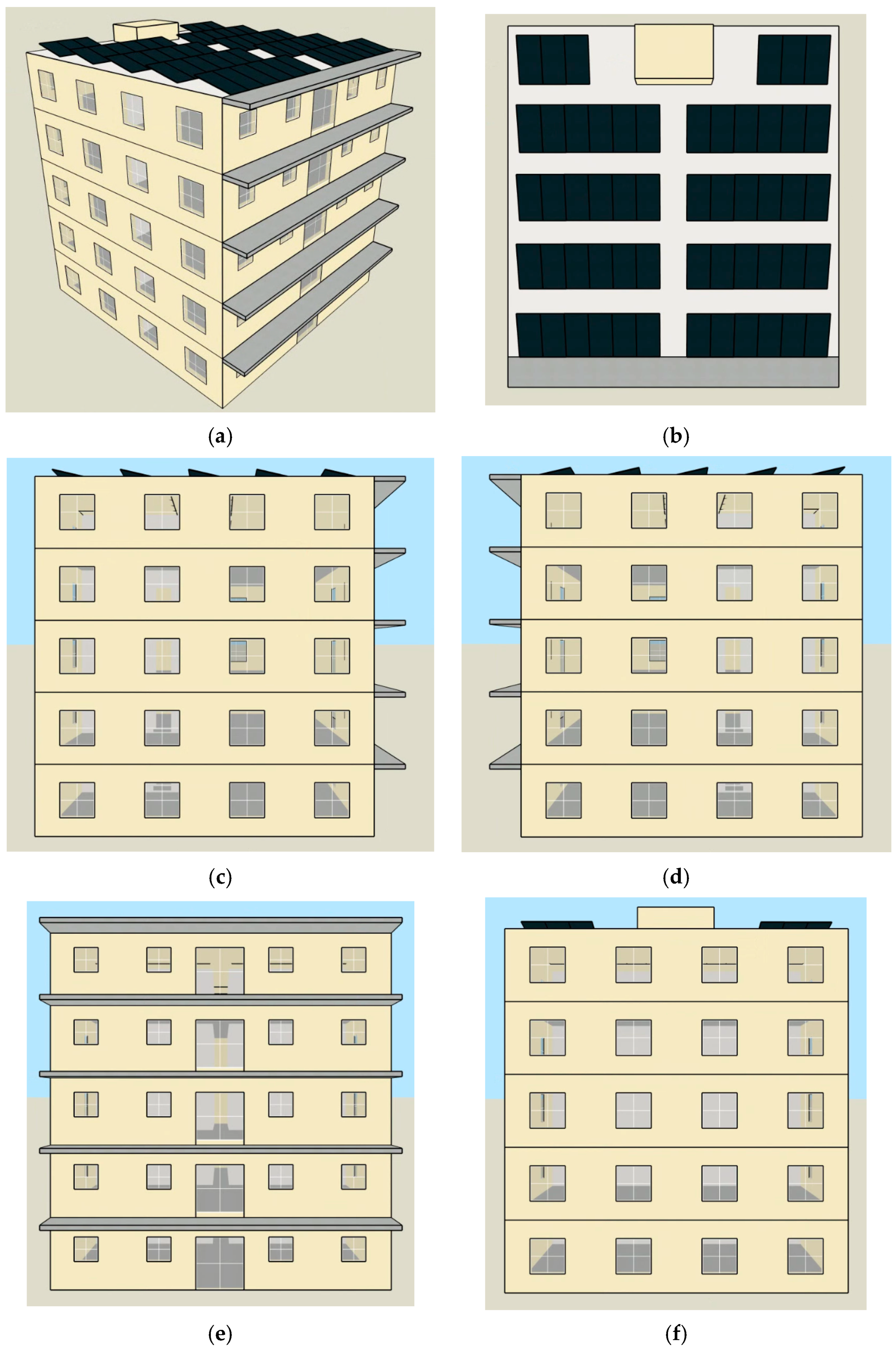
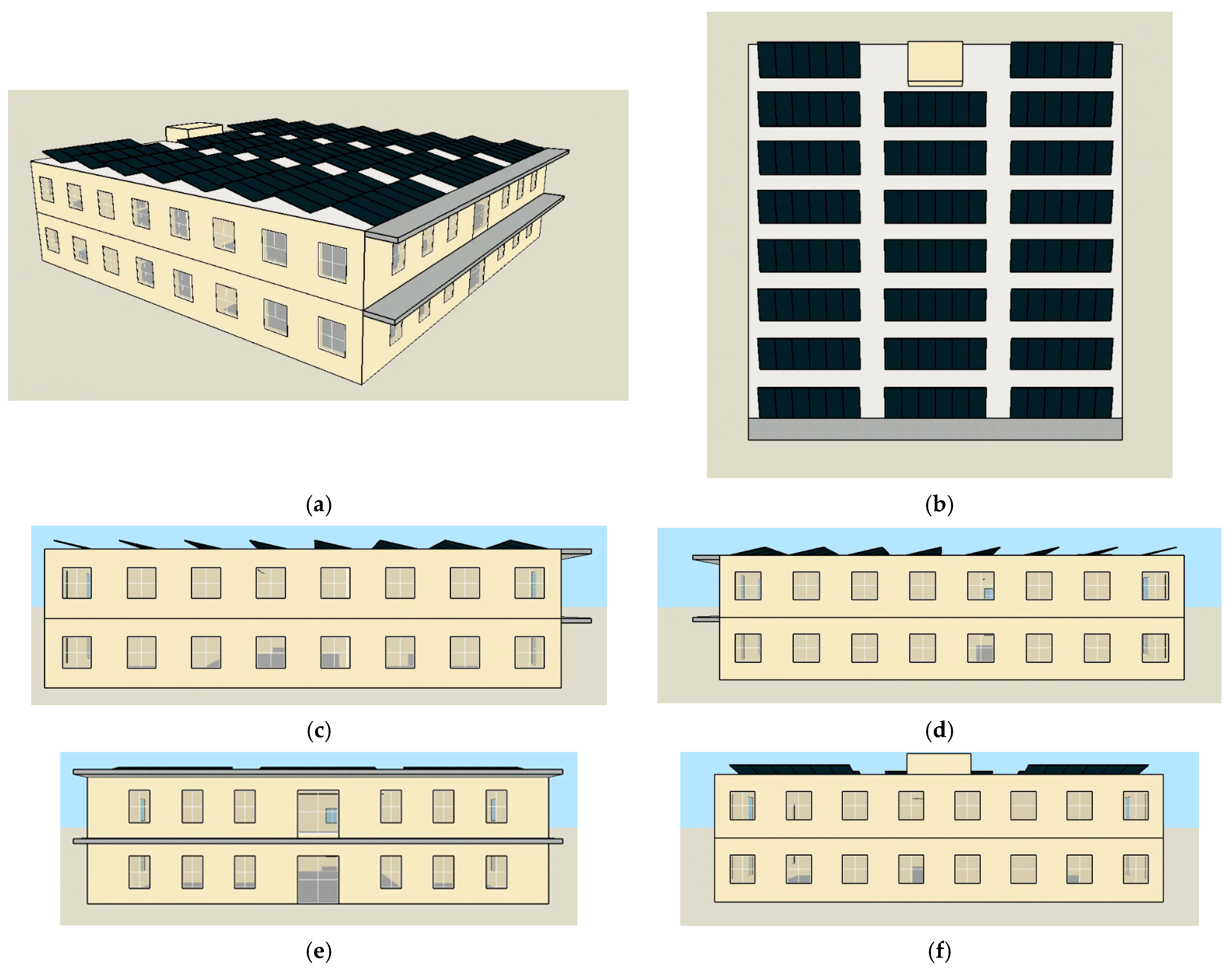
2.1. The Investigated Buildings

2.1.1. Detailed Description of the Buildings and Climatic Conditions

The present energy analysis examines two residential buildings that were designed and simulated in the DesignBuilder v7 software [23]. The building energy analysis was executed with a 5 min timestep, or 12 timestep per hour, which was selected after a sensitivity analysis. Both buildings are characterized by the same gross area of 1000 m² and a total volume of 3000 m³. The first building, referred to as B1, is a five-story multifamily building, with a ground and roof slab area equal to 200 m². The second building, referred to as B2, is a two-story multifamily building, with a five-times-greater ground and a roof slab area of 1000 m². For both buildings, the floor height was considered equal to 3 m, whereas the window-to-wall ratio was selected at 20%. The total building external surface, including the external walls, roof and ground slab, was calculated at 1249 m² and 1537 m² for buildings B1 and B2, respectively, whereas the ratio of total building external surface to volume was calculated at 41.6% for B1 and 51.2% for B2.

Table 1. Basic geometrical dimensions of the examined buildings.

Parameter	Building B1	Building B2
Gross floor area per floor [m2]	200	500
Roof and ground slab area [m2]	200	500
Total building external surface [m2]	1249	1537
Gross exterior wall area [m2]	849	537
Net wall area [m2]	679	429
Total windows area [m2]	170	107
Window-to-wall ratio	0.2	0.2
Number of floors	5	2
Floor height [m]	3	3
Gross building volume [m3]	3000	3000
Ratio of total external surface to volume [m2/m3]	0.416	0.512

gives the basic geometrical dimensions of the examined buildings. Additionally, Figure 1 and Figure 2 depict an axonometric and plan view, as well as each of the four sides of the examined buildings, B1 and B2, that correspond to the four horizon points. The orientation of the examined buildings was considered the same for each of the four investigated locations.

Regarding the operational data of the examined buildings that are summarized in

Table 2. Operational data of each examined building.

Parameter	Value
Winter temperature setpoint	20 °C
Summer temperature setpoint	26 °C
Occupants	30
Thermal load per occupants	80 W/occupant
Specific lighting electrical load	4 W/m2
Specific appliances’ electrical load	2 W/m2
Average operating fraction of the occupants	0.75
Average operating fraction of the lighting	0.75
Average operating fraction of the appliances	0.75
Infiltration rate	0.4 ACH
Natural ventilation rate	0.8 ACH
DHW temperature setpoint	45 °C
DHW demand	50 L/day/person

, each building was occupied by 30 occupants, with a specific thermal load of 80 W per occupant and an average operating factor of 75%. Additionally, the specific load of appliances and lighting was considered equal to 2 and 4 W/m², with an average operating factor of 75%. The transient schedule profiles of the occupants, appliances and lighting were inserted as a daily distribution load profile which was properly adapted to a typical residential operational schedule [24]. The infiltration rate was considered equal to 0.4 air changes per hour (ACH), whereas the ventilation rate was 0.8 ACH. The buildings were equipped with highly efficient reversible water-to-air heat pump units that satisfied the building’s heating and cooling needs through fan coils, as well as the DHW demand. The temperature setpoint was set to 20 °C for the winter period and 26 °C for the summer period. Additionally, the DHW temperature setpoint was set to 45 °C, whereas the daily demand was considered equal to 50 L per person.

The buildings were examined for the climatic data of Athens, Barcelona, Munich and Stockholm.

Table 3. Basic climatic parameters of each examined location.

Parameter	Athens	Barcelona	Munich	Stockholm
Mean yearly air temperature [°C]	18.0	14.6	9.0	7.5
Mean yearly water temperature [°C]	17.0	14.0	8.0	6.5
Total horizontal irradiation [kWh/m2]	1832	1630	1194	997
Heating degree days	1041	1658	3358	3812
Cooling degree days	588	108	11	1

summarizes the basic climatic parameters of each studied location, namely the average annual air and water temperature, the total horizontal irradiation, and the heating and cooling degree days. The meteorological data for each location were retrieved from the DesignBuilder weather library [23]. Moreover, the building’s thermal transmittance value of structural constructions, namely, external walls, windows, and floor and ground slabs were determined by the national guidelines of each respective country.

Table 4. Thermal transmittance (U-value) of structural constructions per city.

	U-Value [W/m2 K]
Structural Construction	Athens	Barcelona	Munich	Stockholm
External Walls	0.45	0.49	0.21	0.18
Roof Slab	0.4	0.4	0.15	0.13
Ground Slab	0.8	0.75	0.263	0.15
Windows	2.6	2.1	1.05	1.2
	Mean U-value of entire thermal envelope [W/m2 K]
Building B1	0.726	0.568	0.676	0.536
Building B2	0.568	0.676	0.536	0.302

includes the thermal transmittance values (U-value) per building construction and city. Additionally, the average thermal transmittance value of the entire thermal cell was calculated for both buildings B1 and B2.

2.1.2. Definition of the Building Envelope U-Values

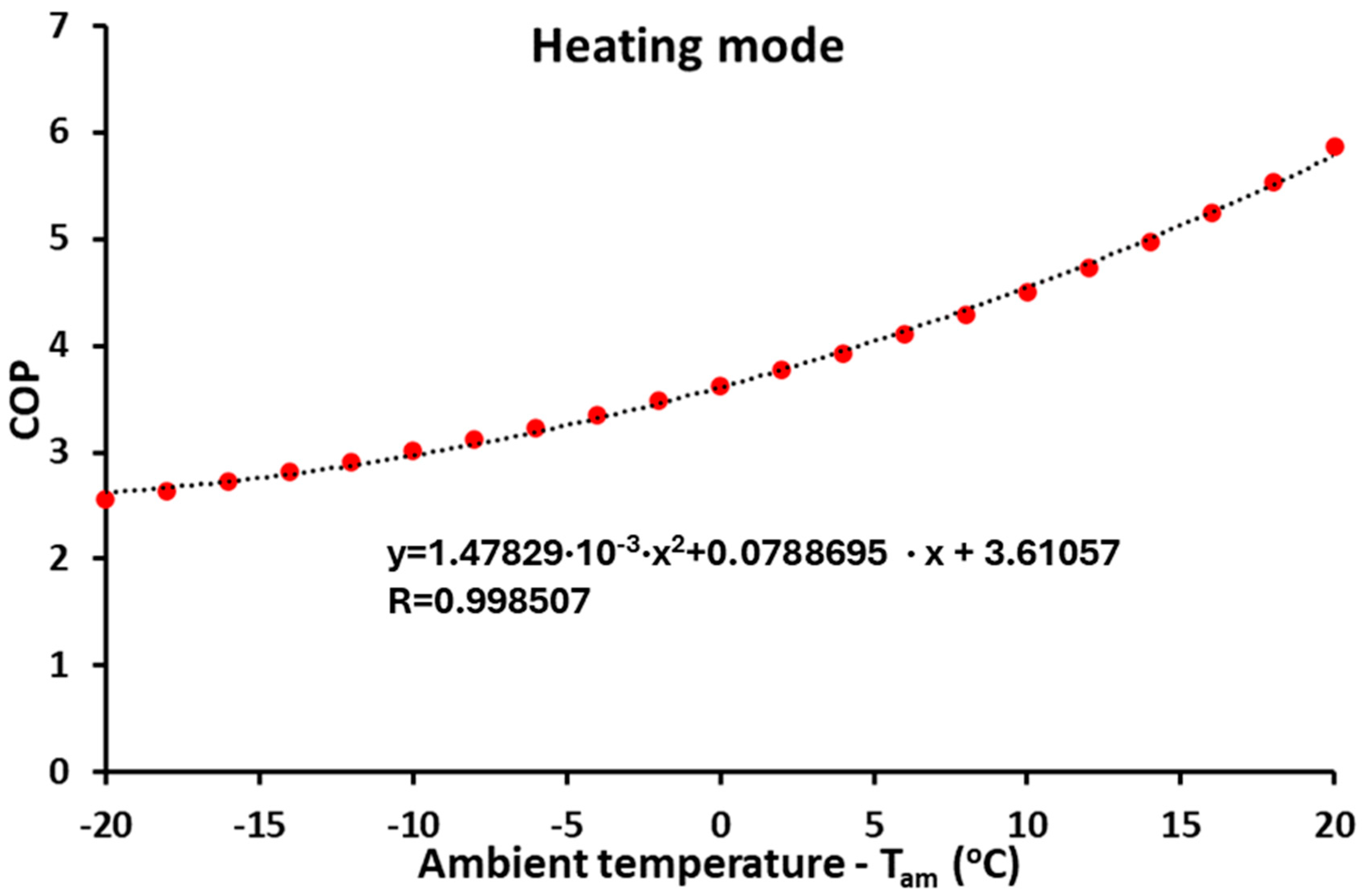
The thermal transmittance [W/m² K] of the building structure, namely walls, roof and ground slab, is found using the following formula [25]:

$$\mathrm{U}={\displaystyle \frac{1}{\frac{1}{{\mathrm{h}}_{\mathrm{in}}}+\sum \frac{{\mathrm{t}}_{\mathrm{i}}}{{\mathrm{k}}_{\mathrm{i}}}+\frac{1}{{\mathrm{h}}_{\mathrm{out}}}}}$$

(1)

where (h_in) and (h_out) are the internal and external surface heat convection coefficients [W/m² K] [26], (t) is the thickness [m] and (k) is the thermal conductivity value [W/mK] of every element (i) that constructs a building element.

The thermal transmittance value of the window construction is calculated according to the following equation [25]:

$${\mathrm{U}}_{\mathrm{window}}={\displaystyle \frac{{\mathrm{A}}_{\mathrm{glass}}\cdot {\mathrm{U}}_{\mathrm{glass}}+{\mathrm{A}}_{\mathrm{frame}}\cdot {\mathrm{U}}_{\mathrm{frame}}+{\mathrm{L}}_{\mathrm{gf}}{\cdot \mathsf{\Psi }}_{\mathrm{gf}}}{{\mathrm{A}}_{\mathrm{glass}}+{\mathrm{A}}_{\mathrm{frame}}}}$$

(2)

where (A_glass) and (A_frame) are the surface area of the window glass and frame, respectively, (U_glass) and (U_frame) are the thermal transmittance value of the window glass–frame, (L_gf) is the thermal bridge length between the window glass–frame, and (Ψ_gf) is the window thermal bridge linear coefficient [W/mK].

The average thermal transmittance value [W/m² K] of the building thermal cell is calculated as follows:

$${\mathrm{U}}_{\mathrm{m}}={\displaystyle \frac{\sum {\mathrm{A}}_{\mathrm{j}}\cdot {\mathrm{U}}_{\mathrm{j}}\cdot {\mathrm{b}}_{\mathrm{j}}+\sum {\mathrm{L}}_{\mathrm{j}}\cdot {\mathsf{\Psi }}_{\mathrm{j}}\cdot {\mathrm{b}}_{\mathrm{tb},\mathrm{j}}}{\sum {\mathrm{A}}_{\mathrm{j}}}}$$

(3)

where (A) is the surface area [m²] occupied by each structural element, (j) is the total area of the building envelope, (U) is the thermal transmittance value [W/m² K] of every construction element, (b) is the reduction coefficient determined by the adjacency condition of the building element [25], (L) the total length [m] of each type of thermal bridge developed in the building envelope, (Ψ) is the linear coefficient of thermal bridge losses [W/mK] and (b_tb) is the respective reduction coefficient.

2.2. HP Modeling

2.2.1. Mathematical Formulation of the Heat Pump

In this work, a reversible air-to-water heat pump was examined, which is coupled with fan coils for heating and cooling production. Figure 3 depicts the basic configuration of a heat pump.

The heat input in the evaporator is given as follows:

$${\mathrm{Q}}_{\mathrm{evap}}=\mathrm{m}\cdot ({\mathrm{h}}_1-{\mathrm{h}}_4)$$

(4)

The state point (1) can be assumed to be a saturated vapor of low pressure.

The work input in the compressor is calculated as follows:

$${\mathrm{W}}_{\mathrm{c}}=\mathrm{m}\cdot ({\mathrm{h}}_2-{\mathrm{h}}_1)$$

(5)

The isentropic efficiency of the compressor is given as follows:

$${\mathsf{\eta }}_{\mathrm{is},\mathrm{c}}={\displaystyle \frac{{\mathrm{h}}_{2_{is}}-{\mathrm{h}}_1}{{\mathrm{h}}_2-{\mathrm{h}}_1}}$$

(6)

The state point (2_is) is the state point with the high pressure of the cycle and specific entropy equal to the respective of the state point (1).

The electricity consumption is calculated as follows:

$${\mathrm{P}}_{\mathrm{el}}={\displaystyle \frac{{\mathrm{W}}_{\mathrm{c}}}{{\mathsf{\eta }}_{\mathrm{motor}}}}$$

(7)

The heat rejection of the condenser is calculated as follows:

$${\mathrm{Q}}_{\mathrm{cond}}=\mathrm{m}\cdot ({\mathrm{h}}_3-{\mathrm{h}}_2)$$

(8)

The state point (3) is assumed to be a saturated liquid of high pressure.

The expansion in the throttling value is assumed to be ideal and thus the process is isenthalpic:

$${\mathrm{h}}_4={\mathrm{h}}_3$$

(9)

During the heating operation, the COP is calculated as follows:

$$\mathrm{COP}={\displaystyle \frac{{\mathrm{Q}}_{\mathrm{cond}}}{{\mathrm{P}}_{\mathrm{el}}}}$$

(10)

During the cooling operation, the EER is calculated as follows:

$$\mathrm{EER}={\displaystyle \frac{{\mathrm{Q}}_{\mathrm{evap}}}{{\mathrm{P}}_{\mathrm{el}}}}$$

(11)

2.2.2. Developed Model for the Heat Pump Simulation

In this work, a thermodynamic model of the heat pump was created in the Engineering Equation Solver (EES) tool [27] for the working fluid (R600) which is a natural refrigerant. The thermodynamic properties of the fluid were found in the tool libraries. The isentropic efficiency was selected at η_is,c = 85% and the motor efficiency at η_motor = 90%, which are typical values.

In the heating mode, the condenser temperature was chosen at 50 °C, while the evaporator temperature was selected to be 7 K lower than the ambient temperature. In this case, the COP was estimated using the (T_am) in [°C] as the parameter, with the following approximation formula:

$$\mathrm{COP}=3.61057+7.88695\cdot {10}^{-2}\cdot {\mathrm{T}}_{\mathrm{am}}+1.47829\cdot {10}^{-3}\cdot {\mathrm{T}}_{\mathrm{am}}^2$$

(12)

The previous formula has a high approximation accuracy of R² = 99.85%. Figure 4 shows the COP variation with the variation in environmental temperature.

In the cooling mode, the evaporator temperature was selected at 0 °C, while the condenser temperature was selected to be 7 K greater than the environmental temperature. In this case, the EER was estimated using the (T_am) in [°C] as the parameter, with the following approximation formula:

$$\mathrm{EER}=18.7896-0.935207\cdot {\mathrm{T}}_{\mathrm{am}}+2.05509\cdot {10}^{-2}\cdot {\mathrm{T}}_{\mathrm{am}}^2-1.66074\cdot {10}^{-4}\cdot {\mathrm{T}}_{\mathrm{am}}^3$$

(13)

The previous formula has a high approximation accuracy of R² = 99.91%. Figure 5 shows the EER variation with the variation in ambient temperature.

2.3. PV Technology Description and Modeling

The modeling of the studied PV was based on the equations given in the next subsections. These equations are mainly energy balances and efficiency definitions.

2.3.1. General Modeling of the PV

The solar irradiation on the collector aperture is calculated as follows:

$${\mathrm{Q}}_{\mathrm{sol}}={\mathrm{A}}_{\mathrm{pv}}\cdot {\mathrm{G}}_{\mathrm{T}}$$

(14)

The produced electricity can be found using the PV electrical efficiency as follows:

$${\mathrm{P}}_{\mathrm{el}}={\mathsf{\eta }}_{\mathrm{pv}}\cdot {\mathrm{Q}}_{\mathrm{sol}}$$

(15)

The PV electrical efficiency can be found according to the following formula [28]:

$${\mathsf{\eta }}_{\mathrm{pv}}={\mathsf{\eta }}_{\mathrm{ref}}\cdot \left[1-\mathsf{\beta }\cdot \left({\mathrm{T}}_{\mathrm{cell}}-{\mathrm{T}}_{\mathrm{am}}\right)\right]$$

(16)

The cell temperature is found as [29]

$${\mathrm{T}}_{\mathrm{cell}}={\mathrm{T}}_{\mathrm{am}}+\mathrm{f}\cdot {\mathrm{G}}_{\mathrm{T}}$$

(17)

The parameter (f) is associated with the nominal operating cell temperature (NOCT), which is the photovoltaic cell temperature level for the environmental temperature of 20 °C, solar irradiation on the titled surface at 800 W/m² and wind velocity at 1 m/s [30]. More specifically, the cell temperature can be found as follows [30]:

$${\mathrm{T}}_{\mathrm{cell}}={\mathrm{T}}_{\mathrm{am}}+{\displaystyle \frac{\mathrm{NOCT}-20}{800}}\cdot {\mathrm{G}}_{\mathrm{T}}$$

(18)

where the parameter (f) can be written as

$$\mathrm{f}={\displaystyle \frac{\mathrm{NOCT}-20}{800}}$$

(19)

Modeling the PV with the use of a constant value of the parameter (f) is an acceptable way, but it suffers from deviations when the operating conditions are not close to the nominal conditions. Therefore, more detailed modeling with thermal losses can be considered in order to take into consideration the different performance enhancement techniques.

The BIPV modeling is performed by using a proper (f) factor according to ref. [29], which is f = 0.0538.

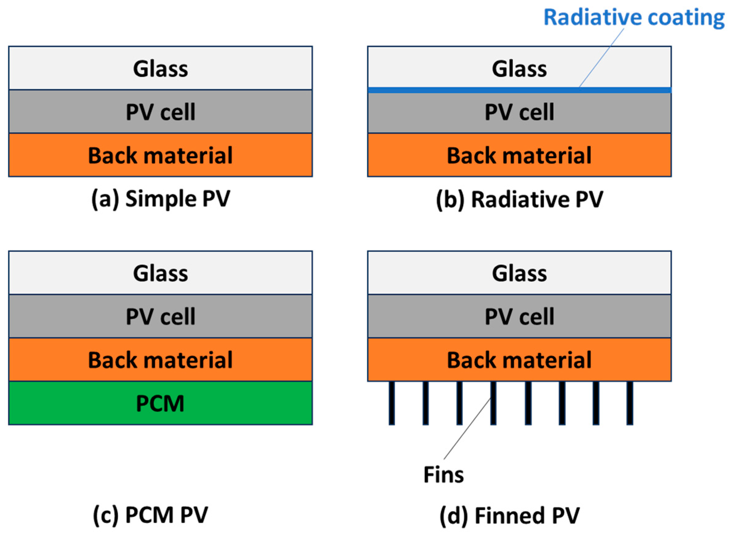
2.3.2. Thermal Modeling of the Simple PV

The simple PV is the conventional PV design and below, a thermal model is given to estimate its performance for different operating conditions by taking into consideration the variation in solar irradiation (G_T), environmental temperature (T_am) and wind speed (V_w).

The absorbed energy by the PV cell (Q_abs) is calculated by considering the optical losses of the cover and the cell surface. The glass transmittance (τ) and the cell absorbance (α) are multiplied by the solar energy as follows:

$${\mathrm{Q}}_{\mathrm{abs}}=\mathsf{\tau }\cdot \mathrm{a}\cdot {\mathrm{Q}}_{\mathrm{sol}}$$

(20)

The energy balance in the PV cell can be expressed by considering that the absorbed solar irradiation is separated into electricity production and into total thermal losses (Q_loss,tot) [29]:

$${\mathrm{Q}}_{\mathrm{abs}}={\mathrm{P}}_{\mathrm{el}}+{\mathrm{Q}}_{\mathrm{loss},\mathrm{tot}}$$

(21)

The electricity production can be found as follows:

$${\mathrm{P}}_{\mathrm{el}}={\mathsf{\eta }}_{\mathrm{ref}}\cdot \left[1-\mathsf{\beta }\cdot \left({\mathrm{T}}_{\mathrm{cell}}-{\mathrm{T}}_{\mathrm{am}}\right)\right]\cdot {\mathrm{Q}}_{\mathrm{sol}}$$

(22)

The total thermal losses (Q_loss,tot) are separated into upper thermal losses (Q_loss,u) and back thermal losses (Q_loss,b):

$${\mathrm{Q}}_{\mathrm{loss},\mathrm{tot}}={\mathrm{Q}}_{\mathrm{loss},\mathrm{u}}+{\mathrm{Q}}_{\mathrm{loss},\mathrm{b}}$$

(23)

The upper thermal losses are calculated by neglecting the conductive effect in the glass due to its very small thickness and its high thermal conductivity. Practically, it is considered that ${\mathrm{T}}_{\mathrm{cell}}\approx {\mathrm{T}}_{\mathrm{glass}}$. The upper thermal losses are separated into convective and radiative thermal losses:

$${\mathrm{Q}}_{\mathrm{loss},\mathrm{u}}={\mathrm{Q}}_{\mathrm{loss},\mathrm{u},\mathrm{conv}}+{\mathrm{Q}}_{\mathrm{loss},\mathrm{u},\mathrm{rad}}$$

(24)

The upper convection thermal losses are calculated as follows:

$${\mathrm{Q}}_{\mathrm{loss},\mathrm{u},\mathrm{conv}}={\mathrm{A}}_{\mathrm{pv}}\cdot {\mathrm{h}}_{\mathrm{u}}\cdot \left({\mathrm{T}}_{\mathrm{cell}}-{\mathrm{T}}_{\mathrm{am}}\right)$$

(25)

The heat convection coefficient is calculated according to the wind speed velocity as follows [31]:

$${\mathrm{h}}_{\mathrm{u}}=5.7+3.8\cdot {\mathrm{V}}_{\mathrm{w}}$$

(26)

The upper radiation thermal losses are calculated as follows:

$${\mathrm{Q}}_{\mathrm{loss},\mathrm{u},\mathrm{rad}}={\mathrm{A}}_{\mathrm{pv}}\cdot {\mathsf{\epsilon }}_{\mathrm{u}}\cdot \mathsf{\sigma }\cdot \left({\mathrm{T}}_{\mathrm{cell}}^4-{\mathrm{T}}_{\mathrm{sky}}^4\right)$$

(27)

where (ε_u) is the upper emittance, (σ) is the Stefan–Boltzmann constant at 5.67·10⁻⁸ W/m² K⁴ and (T_sky) is the sky equivalent temperature which is calculated as follows [32]:

$${\mathsf{{\rm T}}}_{\mathrm{sky}}=0.0558\cdot {\mathrm{T}}_{\mathrm{am}}^{1.5}$$

(28)

The temperature levels that are used in the radiation thermal losses calculation are used in Kelvin units.

The PV cell thermal energy losses from its back surface are equal to the conduction thermal losses through the back material. These thermal losses can be written as follows:

$${\mathsf{{\rm T}}}_{\mathrm{sky}}=0.0558\cdot {\mathrm{T}}_{\mathrm{am}}^{1.5}$$

(29)

where $\left({\mathrm{k}}_{\mathrm{b}}\right)$ is the thermal conductance of the back material, $\left({\mathrm{L}}_{\mathrm{b}}\right)$ is the thickness of the back and (T_b) is the back temperature which comes in touch with the ambient below the PV.

The thermal losses from the back side to the environment are separated into convective and radiative thermal losses as follows:

$${\mathrm{Q}}_{\mathrm{loss},\mathrm{b}}={\mathrm{Q}}_{\mathrm{loss},\mathrm{b},\mathrm{conv}}+{\mathrm{Q}}_{\mathrm{loss},\mathrm{b},\mathrm{rad}}$$

(30)

The back convection thermal losses are calculated as follows:

$${\mathrm{Q}}_{\mathrm{loss},\mathrm{b},\mathrm{conv}}={\mathrm{A}}_{\mathrm{pv}}\cdot {\mathrm{h}}_{\mathrm{b}}\cdot \left({\mathrm{T}}_{\mathrm{b}}-{\mathrm{T}}_{\mathrm{am}}\right)$$

(31)

The heat convection coefficient is calculated according to the wind speed velocity as follows [31]:

$${\mathrm{h}}_{\mathrm{b}}=5.7+3.8\cdot {\mathrm{V}}_{\mathrm{w}}$$

(32)

The back radiation thermal losses are calculated as follows:

$${\mathrm{Q}}_{\mathrm{loss},\mathrm{b},\mathrm{rad}}={\mathrm{A}}_{\mathrm{pv}}\cdot {\mathsf{\epsilon }}_{\mathrm{b}}\cdot \mathsf{\sigma }\cdot \left({\mathrm{T}}_{\mathrm{cell}}^4-{\mathrm{T}}_{\mathrm{am}}^4\right)$$

(33)

Solving all the previous equations together makes it possible to calculate (T_cell) and consequently determine the value of (P_el), avoiding the use of a specific value of the (f) parameter.

2.3.3. Thermal Modeling of the Radiative PV

The only difference in the modeling of the radiative PV can be found in the radiative thermal losses of the upper part with a modified (increased) emittance [16], which is symbolized (ε_u,rad). Therefore, the only revised formula is the following:

$${\mathrm{Q}}_{\mathrm{loss},\mathrm{u},\mathrm{rad}}={\mathrm{A}}_{\mathrm{pv}}\cdot {\mathsf{\epsilon }}_{\mathrm{u},\mathrm{rad}}\cdot \mathsf{\sigma }\cdot \left({\mathrm{T}}_{\mathrm{cell}}^4-{\mathrm{T}}_{\mathrm{sky}}^4\right)$$

(34)

2.3.4. Thermal Modeling of the PCM PV

The application of the PCM in the back part of the PV can give a positive cooling effect, especially in hot operating conditions (e.g., in the summer). The melting temperature of the phase change material is symbolized (T_melt). The PCM material installed in the back part of the PV is considered to be thick enough so that is not totally liquefied during the daily operation of the PV.

In this modeling, the back material comes in touch with the back surface; therefore, the modeling uses the following new boundary condition:

$${\mathrm{T}}_{\mathrm{b}}={\mathrm{T}}_{\mathrm{melt}}$$

(35)

2.3.5. Thermal Modeling of the Finned PV

The incorporation of thin rectangular aluminum fins in the back surface of the PV enables its effective cooling and the reduction in cell temperature. Practically, the use of these fins adds an extra thermal loss effect on the back surface (Q_loss,fin) and the back thermal losses can be written as follows:

$${\mathrm{Q}}_{\mathrm{loss},\mathrm{b}}={\mathrm{Q}}_{\mathrm{loss},\mathrm{b},\mathrm{conv}}+{\mathrm{Q}}_{\mathrm{loss},\mathrm{b},\mathrm{rad}}+{\mathrm{Q}}_{\mathrm{loss},\mathrm{fin}}$$

(36)

The fin thermal losses can be calculated as follows [33]:

$${\mathrm{Q}}_{\mathrm{loss},\mathrm{fin}}={\mathrm{N}}_{\mathrm{fin}}\cdot \sqrt{{\mathrm{h}}_{\mathrm{b}}\cdot {\mathrm{P}}_{\mathrm{fin}}\cdot {\mathrm{A}}_{\mathrm{fin}}\cdot {\mathrm{k}}_{\mathrm{fin}}}\cdot \left({\mathrm{T}}_{\mathrm{b}}-{\mathrm{T}}_{\mathrm{am}}\right)\cdot \tanh \left[\sqrt{{\displaystyle \frac{{\mathrm{h}}_{\mathrm{b}}\cdot {\mathrm{P}}_{\mathrm{fin}}}{{\mathrm{A}}_{\mathrm{fin}}\cdot {\mathrm{k}}_{\mathrm{fin}}}}}\cdot {\mathrm{L}}_{\mathrm{fin}}\right]$$

(37)

where the number of finds (N_fin), the perimeter of every fin (P_fin), the cross-section of the fin (A_fin), the thermal conductivity of fin material (k_fin) and the length of the fin (L_fin) are used in the previous calculation.

The cross-section of the fin (A_fin) and the perimeter of the fin (P_fin) are calculated by using the fin width (W_fin) and the fin thickness (t_fin):

$${\mathrm{A}}_{\mathrm{fin}}={\mathrm{W}}_{\mathrm{fin}}\cdot {\mathrm{t}}_{\mathrm{fin}}$$

(38)

$${\mathrm{P}}_{\mathrm{fin}}=2\cdot \left({\mathrm{W}}_{\mathrm{fin}}+{\mathrm{t}}_{\mathrm{fin}}\right)$$

(39)

2.3.6. Description of the Examined Designs

Figure 6 depicts the four examined PV designs of the present study. Figure 6a shows the conventional or simple PV, Figure 6b shows the radiative PV which has a radiative coating in the upper part of the PV cell, Figure 6c depicts the PCM PV which has a PCM layer at the back of the PV and Figure 6d shows the finned PV which has rectangular fins in the back part of the PV. In the present work, the examined PV is the module SHARP, Sakai, Osaka, Japan, NUSC360|360 W [34] and its characteristics are summarized in

Table 5. Input parameters of the studied photovoltaics.

Parameter	Value
Simple PV
Module length [m]	1.9556
Module width [m]	0.992
Module area, APV [m2]	1.94
Reference efficiency, ηref	0.185
Thermal loss coefficient, β [K−1]	0.0039
Upper emittance, εu	0.7
Down emittance, εd	0.7
Glass transmittance, τ	0.94
Cell absorptance, α	0.92
Back material thermal conductivity, kb [W/mK]	0.15
Back material thickness, tb [m]	0.01
Radiative PV
Upper emittance, εu	0.95
PCM PV
Melting temperature, Tmelt [°C]	25
Finned PV
Number of the fins, Nfin	200
Length of the fin, Lfin [m]	0.12
Width of the fin, Wfin [m]	0.1
Thickness of the fin, tfin [m]	0.005
Thermal conductivity of the fin, kfin [W/mK]	237
BIPV
Module length [m]	1.245
Module width [m]	0.3
Module area, ABIPV [m2]	1.375
Reference efficiency, ηref	0.056
Thermal loss coefficient, β [K−1]	0.0019
PV parameter, f	0.0538

. Also, this table shows the input parameters of the extra-examined PV cases. Moreover, ONYX, Ávila, Spain, BIPV was used in this work [35], and, more specifically, the module 034_N-12450300 with zero transparency.

2.4. Simulation Strategy

In the present work, two different building envelope typologies with the same total net area are examined in four different European locations. The simulation study was carried out with the DesignBuilder tool [23] and the studied buildings satisfy the local energy performance regulations. The examined buildings were equipped with highly efficient air-to-water heat pumps coupled with fan coil terminals, used for both heating and cooling production. Also, the heat pump system covered the building’s domestic hot water demand. The performance of the heat pump depended on the ambient conditions and the variation in COP/EER was simulated by using a detailed thermodynamic model in the EES tool [27]. The performance curves were extracted from this tool and properly inserted in the DesignBuilder tool [23].

Different PV panels were examined, including the basic PV and three PVs with cooling cell configurations. The use of radiative PV, the PCM PV and the finned PV were studied. Also, the use of BIPV was studied in the present work aiming to design zero-energy buildings. The PV panels were simulated by using proper thermal models, as described in the previous sections, in the EES tool [27]. The dynamic analysis of the PV production was simulated in the same tool by importing the weather data of every location retrieved from the PVGIS tool [36]. Finally, the electricity loads of the building and the electricity production of the PV were properly coupled in order to determine the final electricity balances of the system. The modeling of the PVs was based on the equations that are provided in the respective section.

3. Results

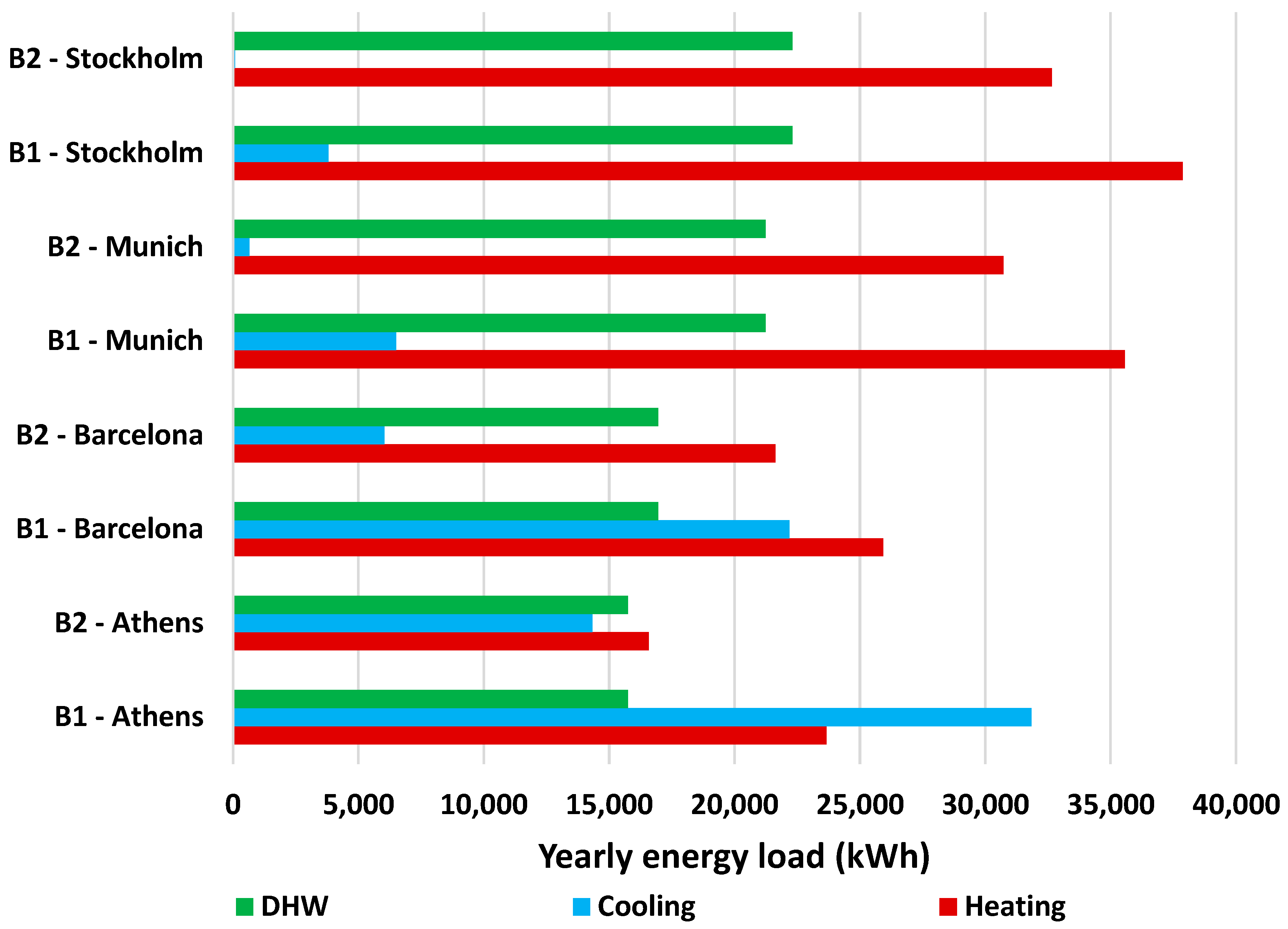
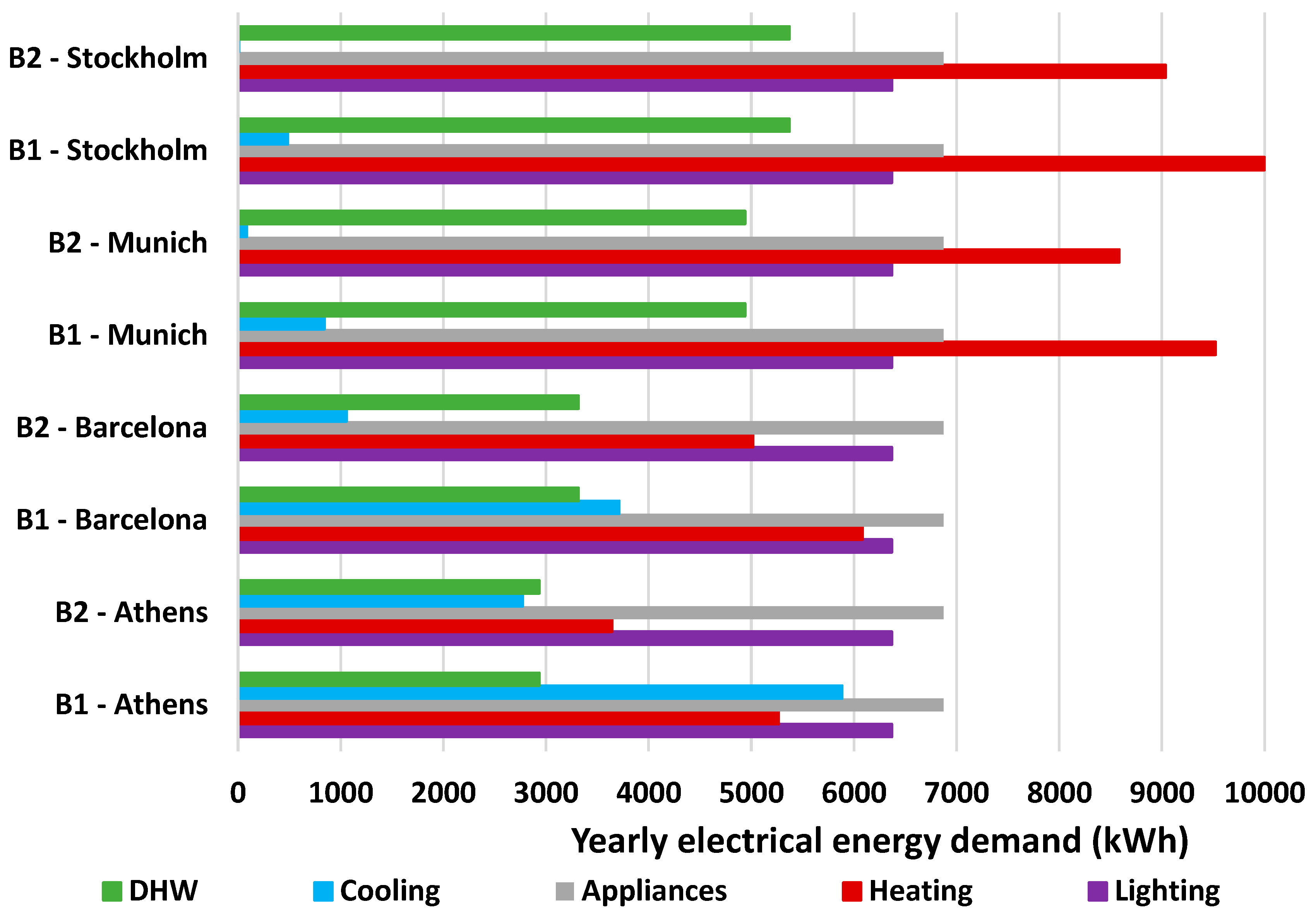
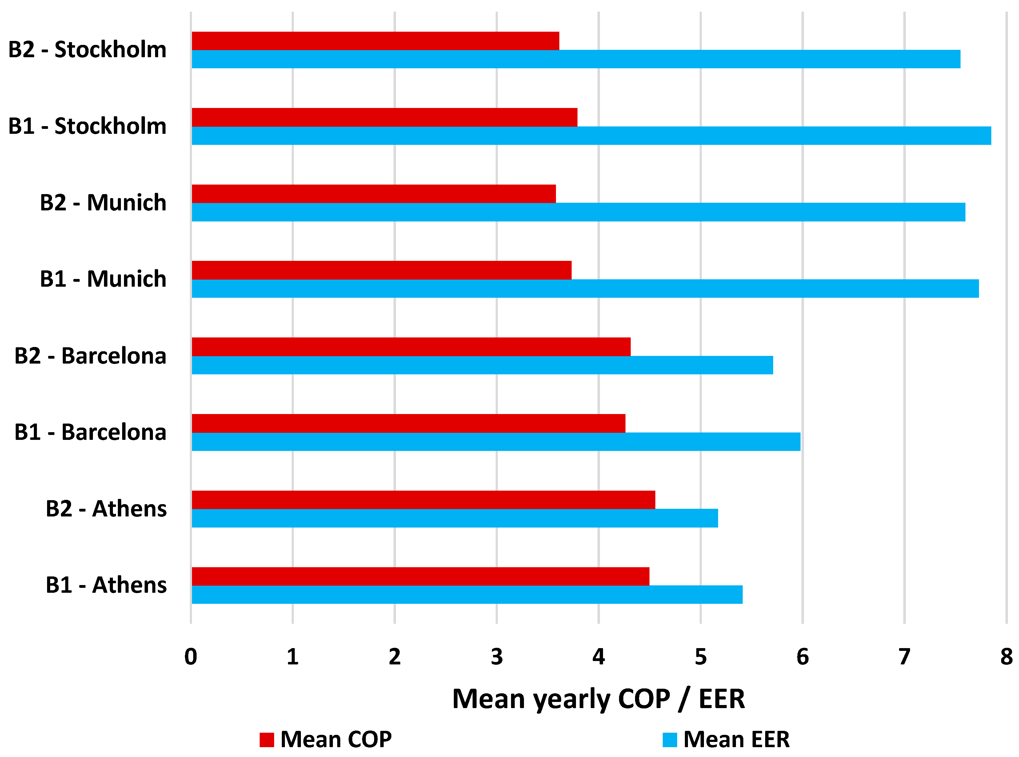
3.1. Energy Analysis of the Examined Buildings at Different Locations

The thermal loads and the energy behavior of the examined buildings are given in this section. Firstly, some indicative results regarding the variation of the loads for the B1 building in Athens are given. Specifically, Figure 7 shows the variation in the heating/cooling thermal loads during the year for this case study. The heating and cooling loads demonstrate similar maximum load values. Specifically, the maximum heating thermal load was 23.1 kW and the maximum cooling thermal load was 21.6 kW. The heating period was equal to 4024 h and the cooling period was a bit shorter equal to 3681 h. Figure 8 depicts the electricity demand of the B1 building in Athens, namely the electricity demand for heating, cooling and the total electricity demands. The total electricity also includes the electricity demand for appliances, lighting and DHW. The maximum total electricity demand was found at 9.1 kW during the winter period. Also, the electrical demands for the heating and cooling of the heat pump were lower compared to the thermal loads because the COP and EER present relatively high values. The seasonal COP was 4.5 and the seasonal EER was 5.4 for the B1 building in Athens.

The next stage is the presentation of the total yearly loads/demands for the eight studied scenarios (two buildings and four locations). Figure 9 illustrates the DHW, heating and cooling loads in each examined case. It is remarkable to state that building B1 had higher cooling loads compared to B2 for all the studied locations. It is interesting to comment that approximately no cooling loads were found for the B2 building in Stockholm. Moreover, the B1 building demonstrated higher heating loads for all the studied locations. The warmer climates (Athens, Barcelona) presented higher cooling loads and lower heating loads compared to the colder climate (Munich, Stockholm): reasonable and acceptable results. Regarding the DHW, there were no important variations among the studied locations, with the warmest climates leading to slightly lower DHW loads.

Figure 10 shows the distribution of the electrical demands for the examined buildings. The DHW electricity demand had a relatively small variation among the examined locations and its demand was higher in colder locations. The electricity demands for lighting and appliances were similar among the examined cases. The electricity demand for covering the cooling load variation was very important among the examined buildings and it was significantly higher in the warmest climates (Athens and Barcelona). On the other hand, the electricity demand for covering the heating demand was higher in the coldest climates (Munich and Stockholm) compared to the other climates. However, the variation in electrical demand for heating was not as intense as the variation in the electrical demand for cooling among the studied scenarios.

Figure 11 depicts the results for the mean COP and EER of the heat pumps for the examined locations. The COP did not present a great fluctuation among the examined cases. However, lower values were presented for the colder ambient conditions. On the other side, the EER presented higher variation and took significantly higher values in colder climates due to the restricted cooling loads and the absence of very warm days.

Table 6. Summary of the loads and the electricity demands for the examined buildings.

Parameter	Athens		Barcelona		Munich		Stockholm
(kWh)	B1	B2	B1	B2	B1	B2	B1	B2
Heating load	23,669	16,585	25,927	21,632	35,570	30,725	37,879	32,651
Cooling load	31,834	14,337	22,191	6038	65,01	645	3799	76
DHW load	15,748	15,748	16,960	16,960	21,236	21,236	22,301	22,301
Electricity for heating	5266	3643	6084	5017	9524	8583	9999	9035
Electricity for cooling	5885	2773	3712	1058	841	85	484	10
Electricity for DHW	2935	2935	3317	3317	4939	4939	5370	5370
Electricity for appliances	6871	6871	6871	6871	6871	6871	6871	6871
Electricity for lighting	6368	6368	6368	6368	6368	6368	6368	6368
Total electricity	27,324	22,590	26,352	22,631	28,543	26,846	29,092	27,654
Mean COP	4.495	4.553	4.262	4.312	3.735	3.580	3.788	3.614
Mean EER	5.410	5.169	5.978	5.709	7.728	7.595	7.848	7.545

summarizes the results for the thermal loads, the electricity production and the efficiency data of the heat pump. Specifically, the heating/cooling loads for Athens B1 were 23,669 kWh and 31,834 kWh, while for B2, they were 16,585 and 14,337, respectively. The total electricity demand was 27,324 kWh and 22,590 kWh for Athens B1 and B2 buildings, respectively. For Barcelona, the heating and cooling loads for B1 were 25,927 kWh and 22,191 kWh, while for B2, they were 21,632 kWh and 6038 kWh, respectively. The total electricity demand is 26,352 kWh and 22,631 kWh for Barcelona B1 and B2 respectively. Regarding Munich, the heating and cooling loads for B1 were 35,570 kWh and 6501 kWh, while for B2, they were 30,725 kWh and 645 kWh, respectively. The total electricity demand was 28,543 kWh and 26,846 kWh for Munich B1 and B2, respectively. Moreover, for Stockholm, the heating and cooling loads for B1 were 3789 kWh and 3799 kWh, while for B2, they were 32,651 kWh and 76 kWh, respectively. The total electricity demand was 29,092 kWh and 27,654 kWh for Stockholm B1 and B2, respectively.

3.2. Parametric Analysis of the PV

The electrical performance of the different examined PV configurations is given in this section. The analysis is parametric and was conducted for various ambient temperatures, from 0 °C up to 35 °C, while two typical incident solar irradiation levels were examined. Specifically, a low solar irradiation level at 400 W/m² and a high solar irradiation level at 800 W/m² were investigated in this parametric work. The application of the different PV cell cooling techniques aimed to reduce cell temperature. Thus, the results of this section regard the cell temperature variation and also the PV electrical performance for the different conditions.

Figure 12 illustrates the cell temperature variation of the different PVs for G_T = 400 W/m² and for different ambient temperatures. For all the PV designs, the rise in the environmental temperature led to higher cell temperature, which is a reasonable result. Moreover, it is interesting that the simple PV led to similar cell temperatures compared to the radiative and the finned cases, with the simple PV presenting a slightly higher cell temperature. Between radiative and finned PV, the finned PV led to a slightly lower temperature but with a very rough difference. On the other hand, the PCM PV had a different behavior and led to a significantly lower cell temperature in colder ambient conditions (approximately up to 20 °C), while in higher ambient temperatures, the PCM PV clearly led to lower efficiencies. These results indicate that the PCM is a very good cooling technique in hot climates. Practically, the melting temperature of the PCM was selected at 25 °C, and in lower ambient temperatures, the PCM existence acted as insulation in the system, blocking the cooling of the photovoltaic cell. However, in higher ambient temperatures, the PCM helped the cell be effectively cooled and not influenced by the warm ambient temperatures.

Figure 13 shows the PV cell electrical efficiency results of the examined cases with G_T = 400 W/m² and for different ambient temperatures. The value of 400 W/m² was selected as a low value of PV incident radiation, representing an average cloudy day. The behavior of the simple, radiative and finned PV demonstrated similar performance, with the finned PV being the most efficient choice, the radiative PV the second choice and the simple being the third choice among them. On the other hand, the PCM PV had a different behavior and was the less efficient choice in the case of low ambient temperatures and the most efficient one in the case of high ambient temperatures. In any case, there were no huge deviations among the examined PVs because the impact of the cell temperature on the results was relatively restricted.

The next figures concern the PV behavior for G_T = 800 W/m². The value of 800 W/m² was selected as a high value of PV incident radiation, representing an average sunny day. Figure 14 shows the cell temperatures and Figure 15 the PV cell electrical efficiency for the studied ambient temperatures. Similar conclusions can be extracted from these figures compared to the respective figures for G_T = 400 W/m² (Figure 12 and Figure 13). However, it is useful to comment that the rise in the solar irradiation produced a higher energy density to the PV; and therefore, the PV cell presents a slightly higher temperature (around 10 K). This fact made the PVs present a slightly lower efficiency in the scenario of high solar irradiation compared to the low irradiation case.

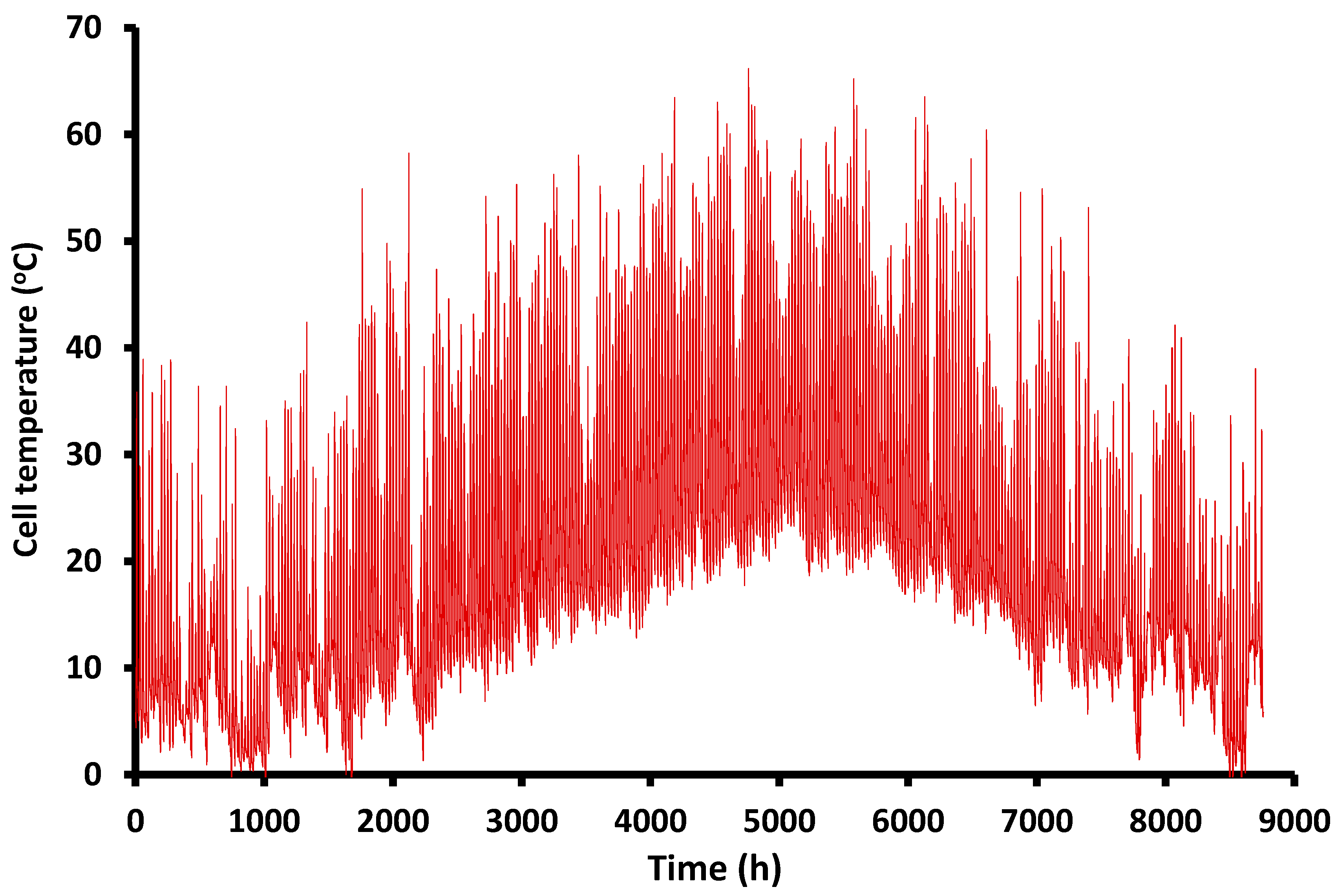
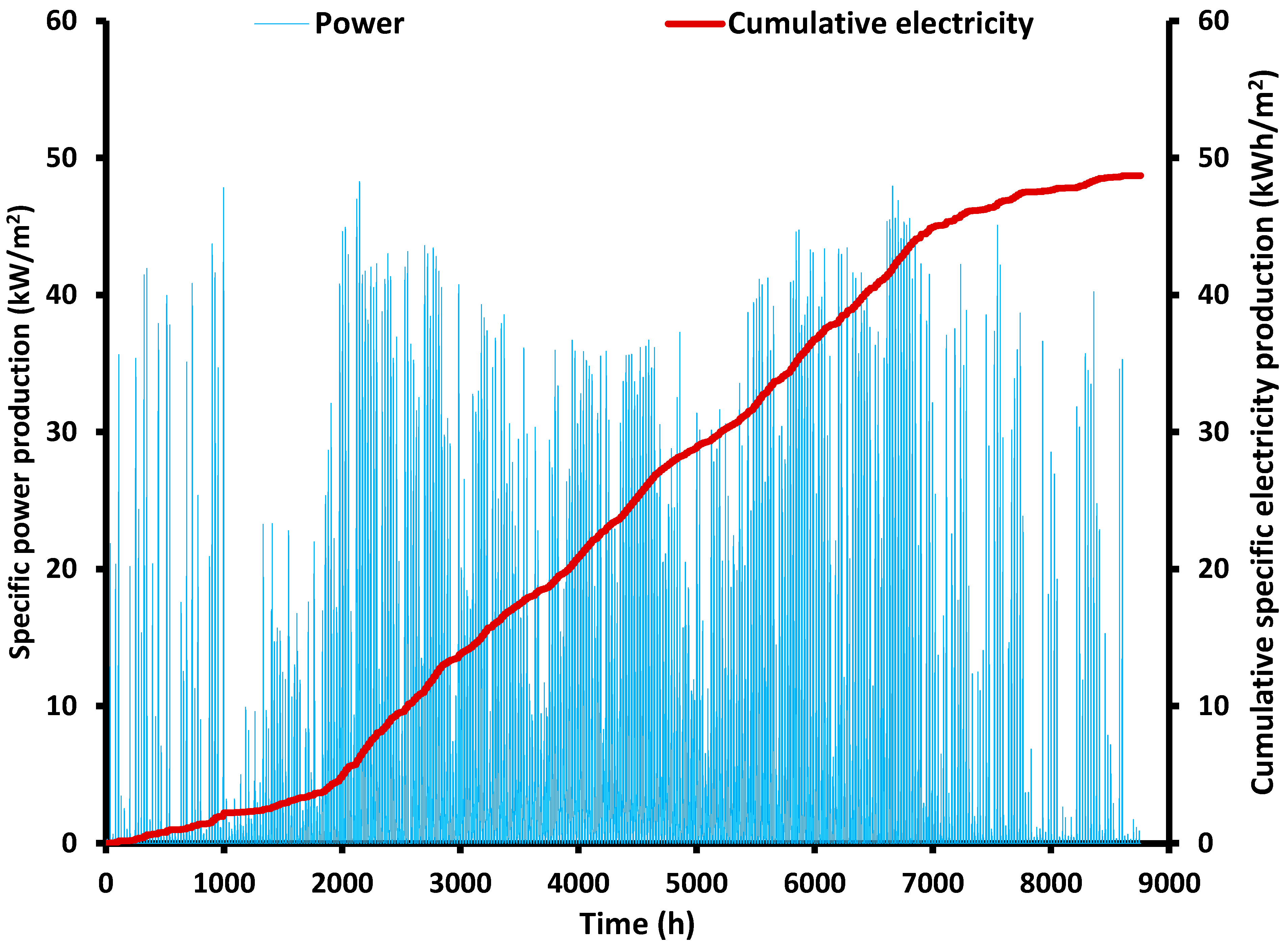
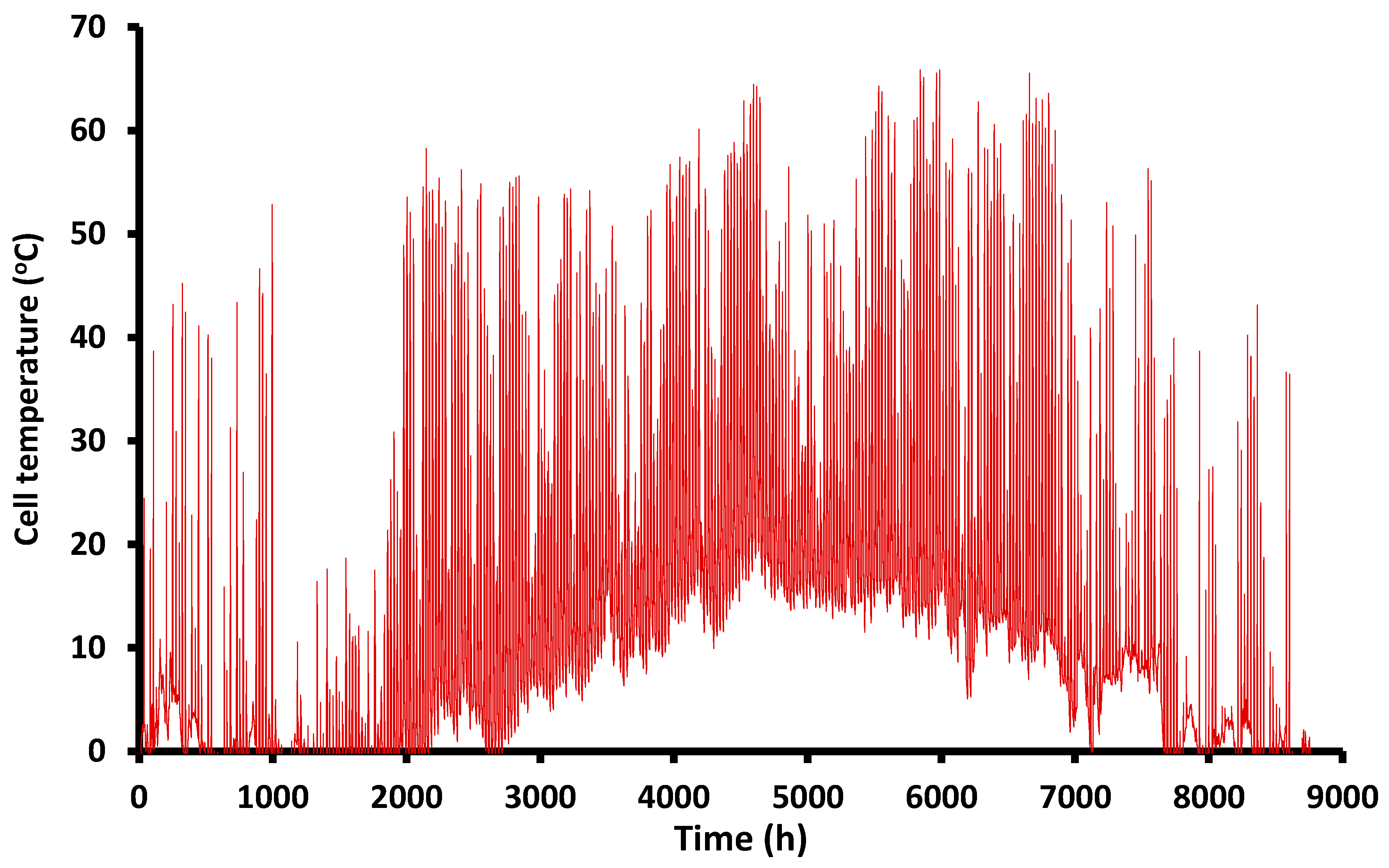
3.3. Dynamic Analysis of the PV—Comparison

The next stage of this simulation concerns the presentation of the electricity production of the investigated PV technologies for the studied scenarios. Firstly, dynamic results of the simulation are presented and after that, the yearly data of the examined cases are given.

Figure 16 and Figure 17 show the yearly variation in simple PV production and the simple PV cell temperatures for the case of Athens. Specifically, Figure 16 shows the hourly PV production per m² and the cumulative electricity production per m². The maximum obtained specific electricity production was 185 W/m², while the cumulative yearly electricity production was about 352 kWh/m². The results indicate that higher production existed during the summer because the production lines were denser and the cumulative curve had a higher slope during the summer. Figure 17 depicts the cell temperature variation of the simple PV for the location of Athens. The maximum cell temperature obtained was 66.2 °C during the summer which is a great temperature level. Hence, there is potential for reducing this temperature level by applying the proper cell cooling techniques.

Figure 18 and Figure 19 illustrate the yearly variation of the BIPV production and the BIPV cell temperatures for the case of Athens. Figure 18 investigates the hourly variation of the specific electricity production of the BIPVs which were mounted on the south side of the building. The maximum specific BIPV production was about 48 W/m², significantly lower than the maximum produced value of the simple PV. This lower value is explained by the significantly lower reference temperature of the BIPV module compared to the simple PV. The cumulative specific electricity production was found at 49 kWh/m², which is lower than the respective for the simple PV for two reasons: the first one is the lower reference efficiency of the BIPV and the second is the lower incident solar potential in the south wall compared to the optimally inclined PV in the roof. Also, the BIPV electricity production was not maximized in the summer because during this period, the solar position was high during the noon and so the solar rays reach the south vertical wall with great incident angle. Figure 19 illustrates the BIPV cell temperature variation during the year. The maximum obtained value was around 65.1 °C, which is similar to the respective maximum value of the simple PV cell temperature.

In the last part of this section, the summary results for eight studied buildings are given in Figure 20 and Figure 21, as well as

Table 7. Summary of the electricity production for the examined buildings.

Parameter	Athens		Barcelona		Munich		Stockholm
(kWh)	B1	B2	B1	B2	B1	B2	B1	B2
Electricity production
Simple PV	35,374	90,400	34,706	88,692	23,505	60,069	21,253	54,313
Radiative PV	35,571	90,905	34,908	89,210	23,671	60,493	21,363	54,595
PCM PV	35,595	90,966	34,714	88,714	23,368	59,717	21,007	53,686
Finned PV	35,619	91,027	34,957	89,335	23,714	60,604	21,376	54,627
BIPV	10,931	6910	11,785	7450	8359	5284	7928	5012
Positive electricity production
Simple PV + BIPV	18,981	74,721	20,139	73,511	3321	38,507	89	31,671
Radiative + BIPV	19,178	75,225	20,341	74,029	3487	38,931	199	31,953
PCM + BIPV	19,202	75,287	20,147	73,533	3184	38,155	−157	31,044
Finned PV + BIPV	19,226	75,347	20,390	74,155	3531	39,042	212	31,985

. The yearly total electricity demand, the simple PV production, the BIPV production and the electricity surplus with the combination of simple PV and BIPV are depicted in Figure 20. In all the cases, the buildings were positive by the combination of BIPV and simple PV. The use of BIPV was needed for having an electricity surplus in the B1 building in the locations of Munich and Stockholm. The highest electricity surpluses were found for the B2 building, while the B1 building had lower electricity surplus values. Moreover, it is interesting to state that the electricity production with simple PV was significantly higher compared to the BIPV production. The PV production was significantly higher in the warmer climates, while the increase in BIPV production in the warm climates was not so intense compared to the coldest climates.

Figure 21 summarizes the results of the application of different PV configurations with integrated cooling techniques compared to the simple PV case. The use of radiative PV and the use of finned PV always led to a higher electricity production. On the other hand, the use of PCM was beneficial in Athens and led to a very small enhancement in Barcelona while it had a negative impact in cold climates (Munich and Stockholm). The maximum enhancements were found for the configuration of finned PV and a slightly lower enhancement with the radiative PV. For Athens, the best option was the application of finned PV with a 0.69% enhancement, the second best was the use of PCM PV with a 0.63% enhancement and the last best cooling technique was the radiative PV with a 0.56% enhancement. The results for Barcelona indicate that for configurations of the finned, radiative and PCM PVs, the respective enhancements were equal to 0.73%, 0.58% and 0.02%. In Munich, finned PVs led to a 0.89% enhancement, the radiative PV to a 0.71% enhancement, while the PCM PV led to a 0.89% decrease in production compared to the simple PV. Also, the results regarding Stockholm highlight the finned PV again as the best choice with a 0.58% enhancement, the radiative PV as the second best with a 0.52% enhancement, and a decrease of 1.15% was found with the use of PCM PV.

These results indicate that relatively low enhancements were achieved with the examined cooling techniques, among which the finned design was declared to be the most appropriate. The PCM addition seemed to only be useful in hot climates and should be avoided in cold climates. In any case, the enhancements of PV production with the incorporation of cooling techniques can lead to positive electricity production and significantly enhance positive electricity production in cold climates. For example, in the case of building B1 in Stockholm, the fined PVs in combination with BIPVs led to a 212 kWh electricity surplus, while the use of simple PVs and BIPV led to an 89 kWh electricity surplus. Therefore, an enhancement of 138% was found in the surplus electricity and this is a very interesting result.

4. Discussion

4.1. Buildings’ Thermal Loads

According to the existing literature, the energy demand for heating and cooling in buildings can vary depending on the climatic characteristics of the location, as well as the construction typology and boundary conditions. Regarding the city of Athens, the specific heating energy demand of the two examined buildings was equal to 23.67 kWh/m² for B1 and 16.59 kWh/m² for B2, while the specific cooling energy demand was calculated at 31.83 kWh/m² for B1 and 14.34 kWh/m² for B2. These results are corroborated by multiple studies that investigate the thermal performance of residencies for the Athenian climatic conditions. Initially, in a study concerning a flat roof single-family house and the implementation of various retrofit techniques, the specific energy demand for heating was found to range between 18.09 kWh/m² and 31.02 kWh/m², while for cooling, it was between 31.65 kWh/m² and 37.21 kWh/m² [37]. Similarly, a study that examined a two-story residential building of 75 m² per story calculated the specific heating energy demand in the range of 21.64 kWh/m² and 26.95 kWh/m², and the specific cooling energy demand in the range of 24.69 kWh/m² and 38.83 kWh/m² [38]. Additionally, for a holistically retrofitted energy-positive four-story multi-family building in Athens, the specific heating/cooling energy demands were calculated at 10.7 kWh/m² and 24.4 kWh/m², respectively [11].

Furthermore, for the Spanish city of Barcelona, the calculated annual specific heating energy demand was found at 25.93 kWh/m² for B1 and 21.63 kWh/m² for B2, and the specific cooling energy demand at 22.19 kWh/m² for B1 and 6.04 kWh/m² for B2. For the Mediterranean Spanish cities, according to the study of Braulio-Gonzalo et al. [39], the annual specific heating demand for a mid-rise multifamily building varies between 27.8 kWh/m² and 68.4 kWh/m² and the specific cooling energy demand between 1.0 kWh/m² and 5.6 kWh/m². Additionally, for a three-story university building with a total floor area of around 4000 m² in the same climatic category as Barcelona, renovated according to the national guidelines of Spain, the specific heating energy demand was around 47 kWh/m² and the specific cooling energy demand was around 18 kWh/m² [40]. For the city of Munich, the calculations of the present analysis indicated a specific energy demand for heating at 35.57 kWh/m² for B1 building and 30.73 kWh/m² for B2, while the cooling demand was found to be 6.5 kWh/m² for B1 and 0.64 kWh/m² for B2. According to the literature, in a two-story single-family house in Munich, the yearly specific heating energy demand was calculated at around 28.0 kWh/m², while the specific cooling energy demand was at 1.5 kWh/m² [41]. Kleinertz et al. [42] examined the energy performance of typical buildings in the city of Munich for various energy standards. According to their calculations, the yearly specific heating energy demand varies between 12.7 kWh/m² for the Passive House standard and 54.5 kWh/m² for the KfW 85 national energy efficiency standard of Germany. For the Swedish city of Stockholm, the yearly energy demand for space heating was calculated at 37.88 kWh/m² for B1 and 32.65 kWh/m² for B2, while the cooling demand was found to be negligible. According to the national technical guidelines of Sweden, the newly constructed residential buildings should not overcome the maximum energy demand for heating at 40 kWh/m² [43] and a total energy performance of 55 kWh/m² [44]. Considering that the examined building was a well-designed one, the slightly lower specific heating demand is reasonable.

4.2. PV Cooling Techniques

Three different cell cooling techniques integrated into a typical PV module were examined with the aim of assisting in the zero-energy transformation of buildings. Their energy performance was strongly dependent on the climatic conditions of the location examined. Despite the slight reported efficiency enhancement, the incorporation of the respective cell cooling techniques can have a decisive impact on the self-sufficiency of a building’s operation. The findings of the present analysis are supported by the existing literature, which verifies the integrity of the calculations of the study.

Firstly, regarding the technological solution of the radiative PV, the results obtained from the present study report a performance enhancement that lies between 0.52%, the poorest performance for the city of Stockholm, and 0.71%, the highest performance for the city of Munich. Similar studies also indicated a slight enhancement in the overall performance of photovoltaic systems through the incorporation of the optically advanced coating solution. Specifically, Nguyen et al. [15] examined the solution of silica multifunctional hybrid structures integrated with radiative cooling coating, and they reported only a marginal improvement of 0.53% regarding the application on solar cells. Similarly, in the study of Zhenpeng et al. [16], the percentage of performance increase attained by the implementation of a radiative coating on a PV module was restricted between 0.43% and 1.07%.

Secondly, the incorporation of PCM in the PV was found to be beneficial only for the hotter climate of Athens, leading to a marginal enhancement of 0.63%. However, the respective solution had an adverse effect on the PV performance for the cities of Barcelona, Munich and Stockholm. Similar conclusions were drawn by Nižetić et al. [20] who concluded that the PCM solution was not always advantageous for the PV performance. Additionally, Ma et al. [17] observed that after a prolonged operation, the PCM-PV system resulted in higher cell temperatures in comparison with the conventional PV cell, which indicates that the use of PCM is not always effective. Lastly, as far as the finned PV construction is concerned, the reported performance enhancement was the highest among the PV cell cooling techniques, lying between 0.58% and 0.89%. The experimental work of Grubišić Čabo et al. [21] concluded that the applications of fins in the backside of the PV can result in performance enhancements of up to 2%. However, these enhancements are dependent on weather conditions, and therefore in some cases, the simple PV configuration is more efficient in contradiction to the finned PV. Also, the specific design of the fins has been found to play a role in the final performance, according to the literature.

5. Conclusions

The development of advanced photovoltaic panels is a critical path for designing zero-energy buildings in the near future. The objective of the present analysis was to examine three promising PV cooling cell designs in different operating conditions and determine the most effective cooling techniques depending on the climate data of every location. The studied cooling techniques were the use of radiative PV cells, the addition of external fins in the down part of the PV and the application of PCM in the down part of the PV. These ideas were systematically compared with the conventional PV design for the climate conditions of Athens, Barcelona, Munich and Stockholm. In every location, two different building typologies were investigated and the goal was to design zero-energy buildings. In the cases that the roof PVs could not cover the total yearly electrical load, BIPVs were also added in the south part of every building. The most remarkable conclusions of the present analysis are summarized as follows:

-

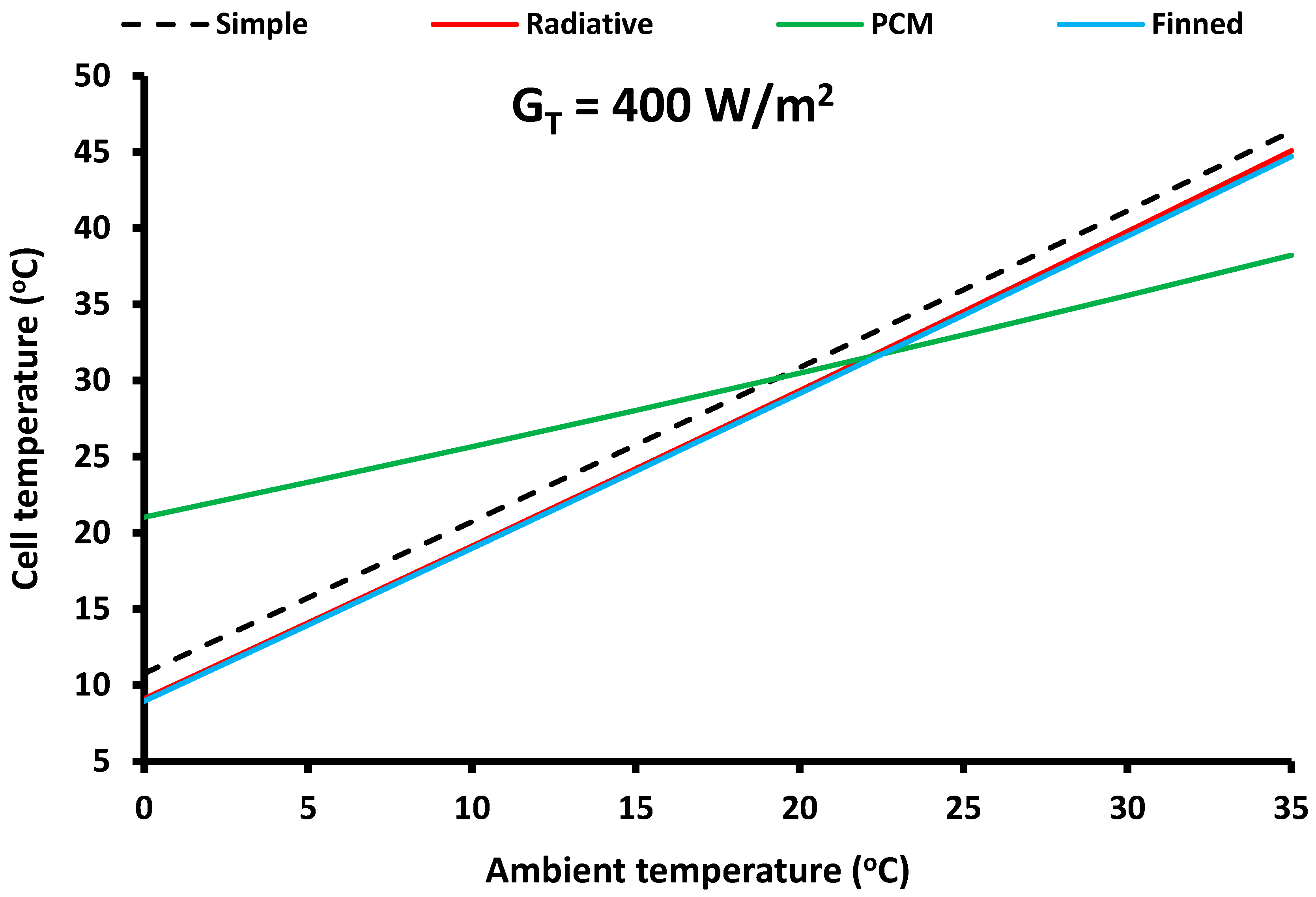
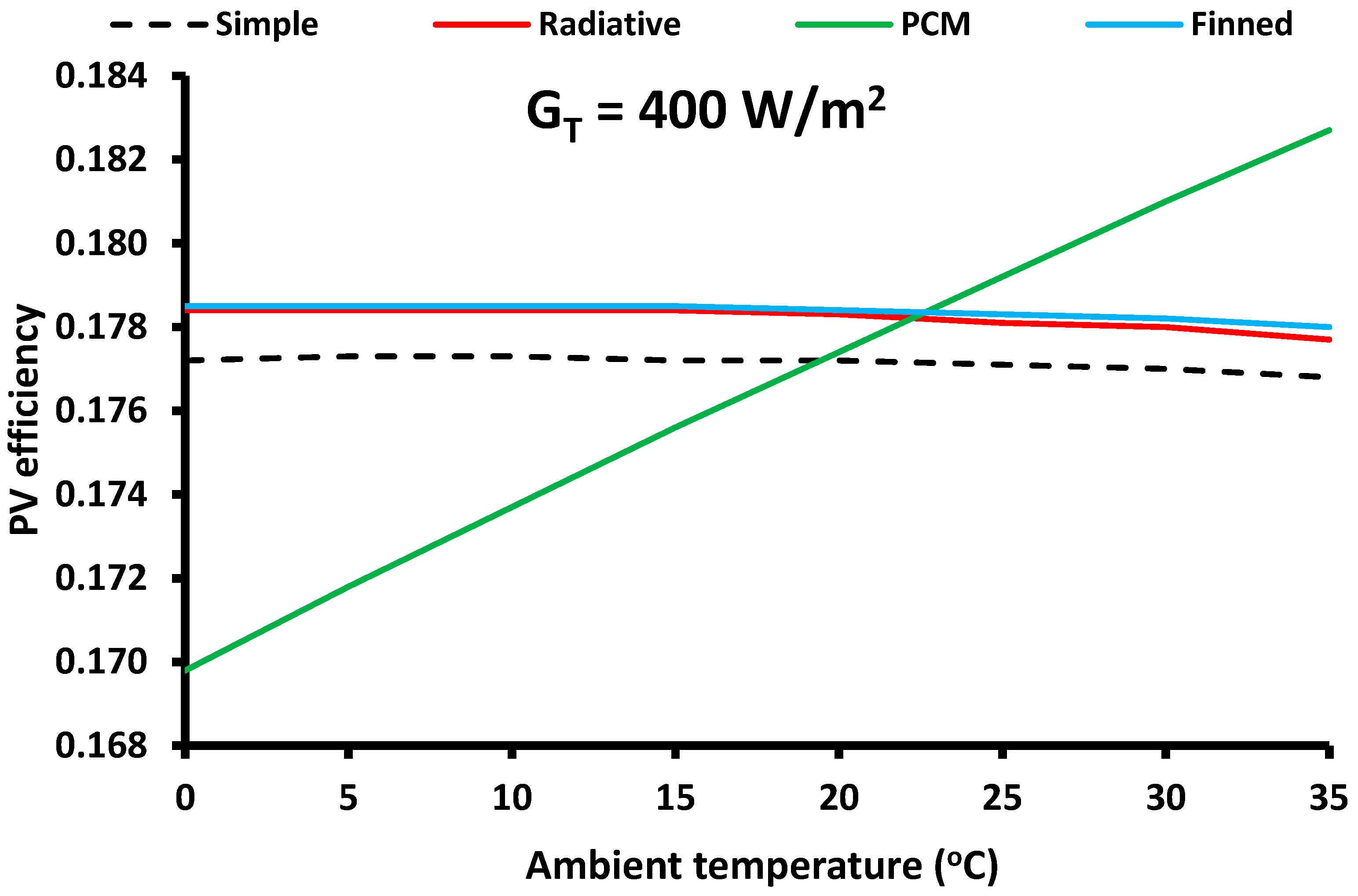
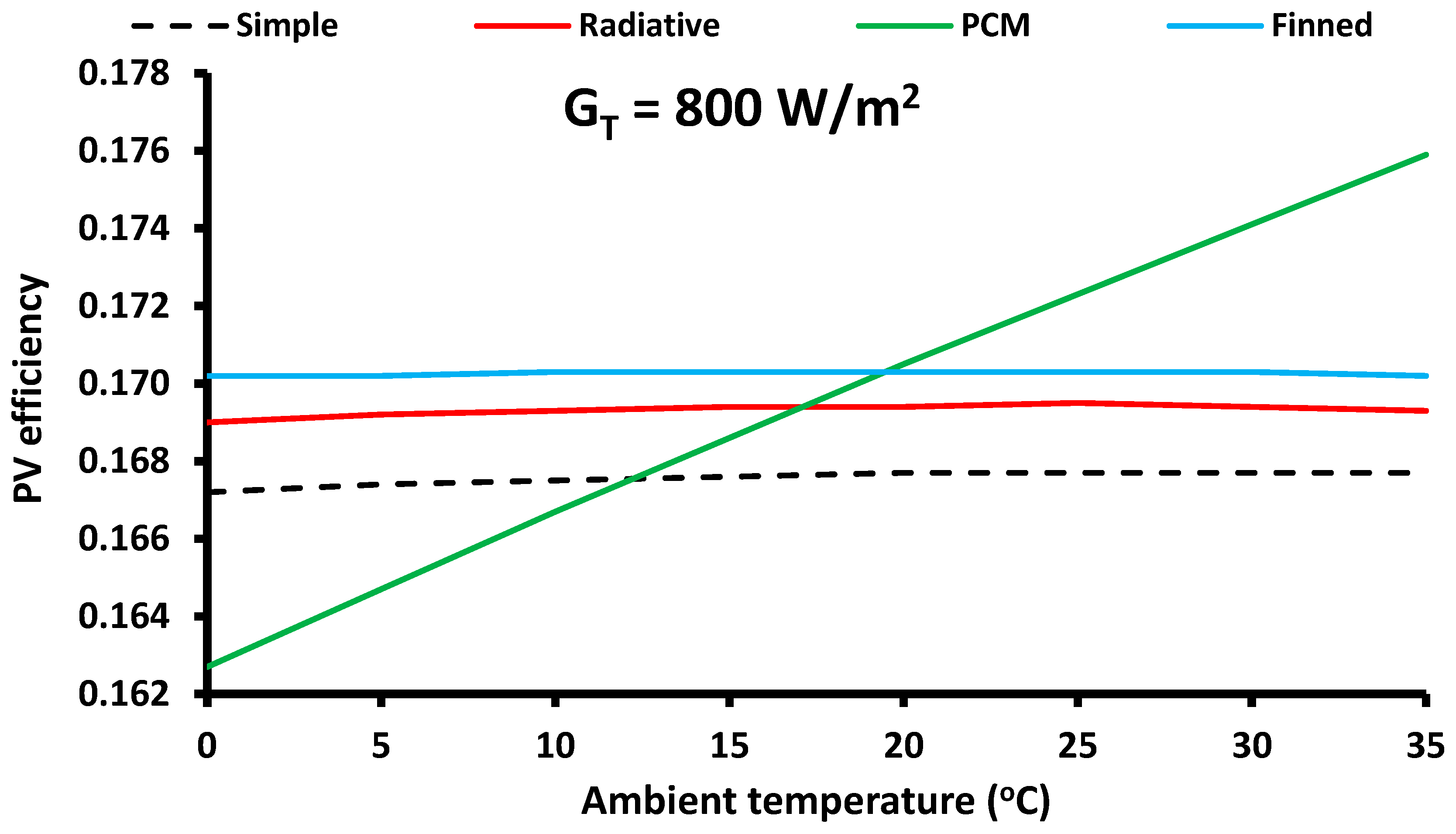
The application of radiative and finned PVs always leads to higher performance compared to simple PV, while the use of PCM has to be selected only in warm climates. The finned PV leads to higher electrical efficiency enhancements which range between 0.58% and 0.89%, while the radiative PVs lead to 0.52% up to 0.71% electrical efficiency enhancements.

-

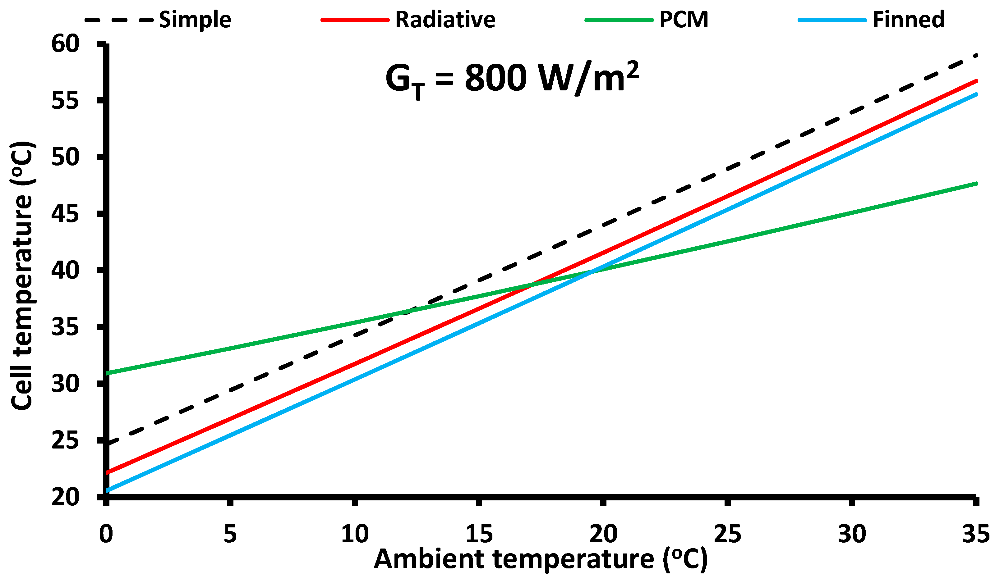
The PCM PVs lead to significantly lower cell temperature levels compared to the other technologies during the summer, but to higher cell temperature levels during the winter. The radiative and the finned designs lead to a bit lower cell temperatures compared to the simple PV configuration.

-

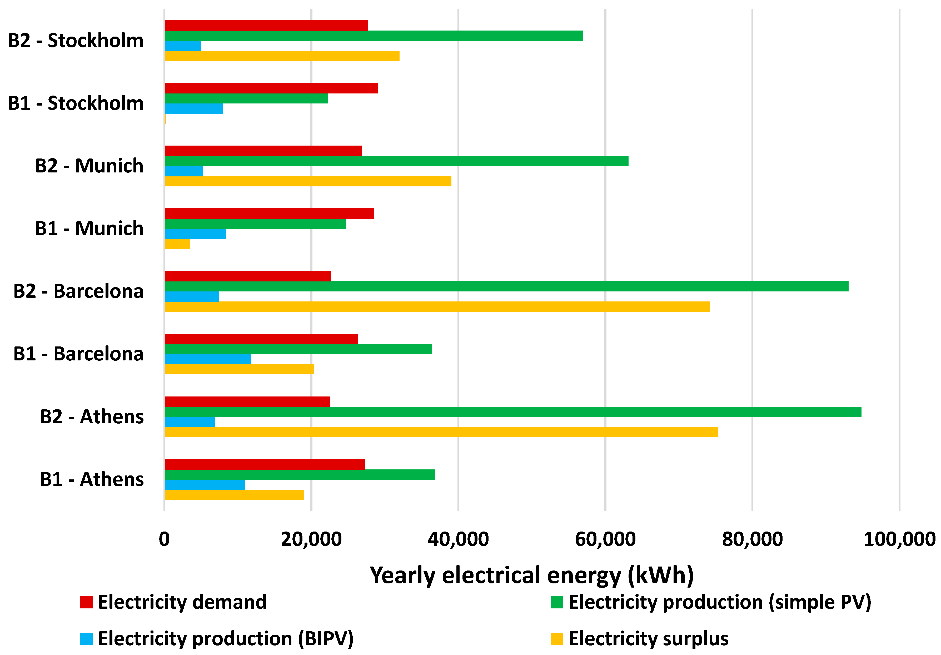
For the climatic conditions of Athens and Barcelona, electrical positivity is achievable only with the use of rooftop PVs, in contrast to Munich and Stockholm, where the use of BIPVs is necessary.

-

The use of the cooling PV designs can significantly enhance positive electricity production in cases with marginal solar potential. Specifically, for building B1 in Stockholm, the fined PVs in combination with BIPVs led to a 212 kWh electricity surplus, or a 136% increase, in contrast to the use of simple PVs in combination with BIPVs.

References

1. Energy Statistics—An Overview. Available online: https://ec.europa.eu/eurostat/statistics-explained/index.php?title=Energy_statistics_-_an_overview (accessed on 29 March 2024).
2. Final Energy Consumption by Energy Sector in EU|ODYSSEE-MURE. Available online: https://www.odyssee-mure.eu/publications/efficiency-by-sector/overview/final-energy-consumption-by-sector.html (accessed on 29 March 2024).
3. Nearly Zero-Energy Buildings. Available online: https://energy.ec.europa.eu/topics/energy-efficiency/energy-efficient-buildings/nearly-zero-energy-buildings_en (accessed on 29 March 2024).
4. Renewables—Energy System. Available online: https://www.iea.org/energy-system/renewables (accessed on 29 March 2024).
5. Share of Electricity Production from Renewables. Available online: https://ourworldindata.org/grapher/share-electricity-renewables (accessed on 29 March 2024).
6. Kim, B.-J.; Kim, S.; Go, M.; Joo, H.-J.; Jeong, J.-W. Applicability Performance Evaluation of Cascade Heat Pump for Building Electrification in Winter. J. Build. Eng. 2024, 82, 108406. [Google Scholar] [CrossRef]
7. Li, Y.; Rosengarten, G.; Stanley, C.; Mojiri, A. Electrification of Residential Heating, Cooling and Hot Water: Load Smoothing Using Onsite Photovoltaics, Heat Pump and Thermal Batteries. J. Energy Storage 2022, 56, 105873. [Google Scholar] [CrossRef]
8. Fedorczak-Cisak, M.; Radziszewska-Zielina, E.; Nowak-Ocłoń, M.; Biskupski, J.; Jastrzębski, P.; Kotowicz, A.; Varbanov, P.S.; Klemeš, J.J. A Concept to Maximise Energy Self-Sufficiency of the Housing Stock in Central Europe Based on Renewable Resources and Efficiency Improvement. Energy 2023, 278, 127812. [Google Scholar] [CrossRef]
9. Kapsalis, V.; Maduta, C.; Skandalos, N.; Bhuvad, S.S.; D’Agostino, D.; Yang, R.J.; Udayraj; Parker, D.; Karamanis, D. Bottom-up Energy Transition through Rooftop PV Upscaling: Remaining Issues and Emerging Upgrades towards NZEBs at Different Climatic Conditions. Renew. Sustain. Energy Transit. 2024, 5, 100083. [Google Scholar] [CrossRef]
10. Bellos, E.; Lykas, P.; Tzivanidis, C. Performance Analysis of a Zero-Energy Building Using Photovoltaics and Hydrogen Storage. Appl. Syst. Innov. 2023, 6, 43. [Google Scholar] [CrossRef]
11. Bellos, E.; Iliadis, P.; Papalexis, C.; Rotas, R.; Mamounakis, I.; Sougkakis, V.; Nikolopoulos, N.; Kosmatopoulos, E. Holistic Renovation of a Multi-Family Building in Greece Based on Dynamic Simulation Analysis. J. Clean. Prod. 2022, 381, 135202. [Google Scholar] [CrossRef]
12. Yu, X.; Chan, J.; Chen, C. Review of Radiative Cooling Materials: Performance Evaluation and Design Approaches. Nano Energy 2021, 88, 106259. [Google Scholar] [CrossRef]
13. Radiative Cooling of Solar Cells. Available online: https://opg.optica.org/optica/fulltext.cfm?uri=optica-1-1-32&id=296235 (accessed on 18 April 2024).
14. Zhao, B.; Hu, M.; Ao, X.; Chen, N.; Pei, G. Radiative Cooling: A Review of Fundamentals, Materials, Applications, and Prospects. Appl. Energy 2019, 236, 489–513. [Google Scholar] [CrossRef]
15. Nguyen, H.T.; Nguyen, T.T.; Tran, T.T.; Bang, J.; Kumar, M.; Kim, J.; Yun, J.-H. Colour-Passive Radiative Cooling in Optoelectronics with Silver/Quantum Dot Decorated Silica Multifunctional Hybrid Structures. Chem. Eng. J. 2024, 488, 150840. [Google Scholar] [CrossRef]
16. Li, Z.; Ahmed, S.; Ma, T. Investigating the Effect of Radiative Cooling on the Operating Temperature of Photovoltaic Modules. Sol. RRL 2021, 5, 2000735. [Google Scholar] [CrossRef]
17. Ma, T.; Zhao, J.; Li, Z. Mathematical Modelling and Sensitivity Analysis of Solar Photovoltaic Panel Integrated with Phase Change Material. Appl. Energy 2018, 228, 1147–1158. [Google Scholar] [CrossRef]
18. Sharma, A.; Tyagi, V.V.; Chen, C.R.; Buddhi, D. Review on Thermal Energy Storage with Phase Change Materials and Applications. Renew. Sustain. Energy Rev. 2009, 13, 318–345. [Google Scholar] [CrossRef]
19. Arıcı, M.; Bilgin, F.; Nižetić, S.; Papadopoulos, A.M. Phase Change Material Based Cooling of Photovoltaic Panel: A Simplified Numerical Model for the Optimization of the Phase Change Material Layer and General Economic Evaluation. J. Clean. Prod. 2018, 189, 738–745. [Google Scholar] [CrossRef]
20. Nižetić, S.; Arıcı, M.; Bilgin, F.; Grubišić-Čabo, F. Investigation of Pork Fat as Potential Novel Phase Change Material for Passive Cooling Applications in Photovoltaics. J. Clean. Prod. 2018, 170, 1006–1016. [Google Scholar] [CrossRef]
21. Grubišić Čabo, F.; Nižetić, S.; Giama, E.; Papadopoulos, A. Techno-Economic and Environmental Evaluation of Passive Cooled Photovoltaic Systems in Mediterranean Climate Conditions. Appl. Therm. Eng. 2020, 169, 114947. [Google Scholar] [CrossRef]
22. Li, J.; Zhou, Y.; Niu, X.; Sun, S.; Xu, L.; Jian, Y.; Cheng, Q. Performance Evaluation of Bifacial PV Modules Using High Thermal Conductivity Fins. Sol. Energy 2022, 245, 108–119. [Google Scholar] [CrossRef]
23. DesignBuilder Software Ltd.—Home. Available online: https://designbuilder.co.uk/ (accessed on 17 January 2023).
24. Kitsopoulou, A.; Bellos, E.; Sammoutos, C.; Lykas, P.; Vrachopoulos, M.G.; Tzivanidis, C. A Detailed Investigation of Thermochromic Dye-Based Roof Coatings for Greek Climatic Conditions. J. Build. Eng. 2024, 84, 108570. [Google Scholar] [CrossRef]
25. Technical Guidelines of Technical Chamber of Greece. TEE 2020. Available online: https://web.tee.gr/ (accessed on 12 March 2024).
26. ISO 6946:2017. Available online: https://www.iso.org/standard/65708.html (accessed on 15 March 2024).
27. EES: Engineering Equation Solver|F-Chart Software: Engineering Software. Available online: https://fchartsoftware.com/ees/ (accessed on 19 March 2024).
28. Evans, D.L. Simplified Method for Predicting Photovoltaic Array Output. Sol. Energy 1981, 27, 555–560. [Google Scholar] [CrossRef]
29. Skoplaki, E.; Palyvos, J.A. Operating Temperature of Photovoltaic Modules: A Survey of Pertinent Correlations. Renew. Energy 2009, 34, 23–29. [Google Scholar] [CrossRef]
30. Sun, V.; Asanakham, A.; Deethayat, T.; Kiatsiriroat, T. Evaluation of Nominal Operating Cell Temperature (NOCT) of Glazed Photovoltaic Thermal Module. Case Stud. Therm. Eng. 2021, 28, 101361. [Google Scholar] [CrossRef]
31. Bellos, E.; Tzivanidis, C.; Nikolaou, N. Investigation and Optimization of a Solar Assisted Heat Pump Driven by Nanofluid-Based Hybrid PV. Energy Convers. Manag. 2019, 198, 111831. [Google Scholar] [CrossRef]
32. Swinbank, W.C. Long-wave radiation from clear skies. Q. J. R. Meteorol. Soc. 1963, 89, 339–348. [Google Scholar] [CrossRef]
33. Lienhard, J.H., IV.; Lienhard, J.H., V. A Heat Transfer Textbook, 5th ed.; Dover Publications: Miniola, NY, USA, 2019. [Google Scholar]
34. Homepage. Available online: https://www.sharp.eu/ (accessed on 23 February 2024).
35. Photovoltaic Glass for Buildings—Onyx Solar. Available online: https://onyxsolar.com/ (accessed on 1 March 2024).
36. JRC Photovoltaic Geographical Information System (PVGIS)—European Commission. Available online: https://re.jrc.ec.europa.eu/pvg_tools/en/ (accessed on 19 March 2024).
37. Kitsopoulou, A.; Bellos, E.; Lykas, P.; Vrachopoulos, M.G.; Tzivanidis, C. Multi-Objective Evaluation of Different Retrofitting Scenarios for a Typical Greek Building. Sustain. Energy Technol. Assess. 2023, 57, 103156. [Google Scholar] [CrossRef]
38. Kitsopoulou, A.; Ziozas, N.; Iliadis, P.; Bellos, E.; Tzivanidis, C.; Nikolopoulos, N. Energy Performance Analysis of Alternative Building Retrofit Interventions for the Four Climatic Zones of Greece. J. Build. Eng. 2024, 87, 109015. [Google Scholar] [CrossRef]
39. Braulio-Gonzalo, M.; Bovea, M.D.; Ruá, M.J.; Juan, P. A Methodology for Predicting the Energy Performance and Indoor Thermal Comfort of Residential Stocks on the Neighbourhood and City Scales. A Case Study in Spain. J. Clean. Prod. 2016, 139, 646–665. [Google Scholar] [CrossRef]
40. Sierra-Pérez, J.; Rodríguez-Soria, B.; Boschmonart-Rives, J.; Gabarrell, X. Integrated Life Cycle Assessment and Thermodynamic Simulation of a Public Building’s Envelope Renovation: Conventional vs. Passivhaus Proposal. Appl. Energy 2018, 212, 1510–1521. [Google Scholar] [CrossRef]
41. Quintana-Gallardo, A.; Schau, E.M.; Niemelä, E.P.; Burnard, M.D. Comparing the Environmental Impacts of Wooden Buildings in Spain, Slovenia, and Germany. J. Clean. Prod. 2021, 329, 129587. [Google Scholar] [CrossRef]
42. Kleinertz, B.; Timpe, C.; Bürger, V.; Cludius, J.; Ferstl, J. Analysis of the Cost-Optimal Heat Supply Strategy for Munich Following a Clean Energy Transformation Pathway. Energy Policy 2024, 188, 113968. [Google Scholar] [CrossRef]
43. Shahrokni, H.; Levihn, F.; Brandt, N. Big Meter Data Analysis of the Energy Efficiency Potential in Stockholm’s Building Stock. Energy Build. 2014, 78, 153–164. [Google Scholar] [CrossRef]
44. Golzar, F.; Silveira, S. Impact of Wastewater Heat Recovery in Buildings on the Performance of Centralized Energy Recovery—A Case Study of Stockholm. Appl. Energy 2021, 297, 117141. [Google Scholar] [CrossRef]
Figure 1. Depiction of examined building B1: (a) south–east axonometric view, (b) plan view, (c) east side, (d) west side, (e) south side and (f) north side.
Applsci 14 08950 g001
Figure 2. Depiction of examined building B2: (a) south–east axonometric view, (b) plan view, (c) east side, (d) west side, (e) south side and (f) north side.
Applsci 14 08950 g002
Figure 3. Basic configuration of a heat pump: (a) p-h depiction; (b) T-s depiction.
Applsci 14 08950 g003
Figure 4. COP in the heating mode for different ambient temperature levels.
Applsci 14 08950 g004
Figure 5. EER in the cooling mode for different ambient temperature levels.
Applsci 14 08950 g005
Figure 6. The examined PV designs.
Applsci 14 08950 g006
Figure 7. Yearly variation in the heating and cooling thermal loads for building B1 in Athens.
Applsci 14 08950 g007
Figure 8. Yearly variation in electricity demand for heating, cooling and in total for building B1 in Athens.
Applsci 14 08950 g008
Figure 9. Yearly thermal load of DHW, cooling and heating for all the examined buildings and locations.
Applsci 14 08950 g009
Figure 10. Yearly electrical energy demands for all the examined buildings and locations.
Applsci 14 08950 g010
Figure 11. Yearly mean COP and EER for all the examined buildings and locations.
Applsci 14 08950 g011
Figure 12. Cell temperature variation of the examined PVs for different ambient temperatures and low incident irradiation level at 400 W/m2.
Applsci 14 08950 g012
Figure 13. PV efficiency variation of the examined PVs for different ambient temperatures and low incident irradiation level at 400 W/m2.
Applsci 14 08950 g013
Figure 14. Cell temperature variation of the examined PVs for different ambient temperatures and high incident irradiation level at 800 W/m2.
Applsci 14 08950 g014
Figure 15. PV efficiency variation of the examined PVs for different ambient temperatures and high incident irradiation level at 800 W/m2.
Applsci 14 08950 g015
Figure 16. Yearly variation in specific electricity production for the simple PV in Athens and cumulative specific electricity production.
Applsci 14 08950 g016
Figure 17. Yearly variation in cell temperature for the simple PV in Athens.
Applsci 14 08950 g017
Figure 18. Yearly variation in specific electricity production for the BIPV in Athens and cumulative specific electricity production.
Applsci 14 08950 g018
Figure 19. Yearly variation in cell temperature for the BIPV in Athens.
Applsci 14 08950 g019
Figure 20. Yearly electrical energy for the demand, production by the simple PV, production by the BIP and total electrical surplus for all the examined buildings and locations.
Applsci 14 08950 g020
Figure 21. Yearly electrical energy production variation with radiative, PCM and finned PV compared to the simple PV for all the examined locations.
Applsci 14 08950 g021