Abstract
Tool wear state recognition is a challenging problem because the various types of signals corresponding to different wear states have similar features, making classification difficult. Convolutional neural networks are widely used in the field of tool wear state recognition. To address this problem, this study proposes a milling cutter wear state monitoring model that combines KANS and deep residual networks (ResNet). The traditional ResNet-34’s top linear classifier was replaced with a nonlinear convolutional classifier including _top_kan, and the data were preprocessed using continuous wavelet transform (CWT) to enhance the model’s immunity to interference and feature characterization. The experimental results based on the PHM dataset show that the improved KANS-ResNet-34 model improves accuracy by 1.07% compared to ResNet-34, making it comparable to ResNet-50, while its computation time is only 1/33.68 of the latter. This significantly improves computational efficiency, reduces the pressure on hardware resources, and provides an effective tool wear state recognition solution.
1. Introduction
Tool wear is a naturally occurring phenomenon during cutting and machining, caused by the interaction of unavoidable chemical, mechanical, and physical factors. If this problem is not diagnosed and addressed promptly, it may lead to abnormal cutting conditions, potentially affecting machining efficiency and quality in serious cases [1,2]. Implementing an effective tool condition monitoring system can improve surface quality, increase productivity, and reduce machining costs. Panda et al. found that machining costs can be reduced by more than 30% [3,4].
Currently, there are two main types of tool condition monitoring systems: direct and indirect systems. Although direct monitoring is highly accurate, it must be stopped during monitoring, making it cumbersome and complex, with little significance for actual processing. Indirect monitoring, on the other hand, utilizes multi-signal fusion technology, selecting various monitoring signals such as acoustic emission, vibration, and current signals. These signals are input into different models for comparison and analysis, which then output the corresponding tool wear state [3,5].
In indirect monitoring, the choice of neural network models, such as support vector machines (SVMs), long short-term memory (LSTM) networks, and convolutional neural networks (CNNs), often influences the performance of the monitoring system. Kong et al. [6] used sensors to collect cutting force signals from a machine tool during end milling, extracted features in the frequency, time, and time–frequency domains, and proposed a Whale optimization algorithm (WOA)–support vector machines (SVMs) model to analyze these features for monitoring tool wear. Pu X et al. [7] analyzed the vibration signals in both time and frequency domains and used LSTM networks in conjunction with the constructed time series dataset to analyze the wear of a single-edged hob. Gyeongho et al. [8] utilized a Bayesian approach combined with a convolutional neural network (CNN) to provide uncertainty sensing for a tool-monitoring system.
In recent years, multisensor fusion has become increasingly important in the field of monitoring and identification, as it allows for the complementary use of information from multiple sensors [9,10]. Serin [9] utilized four key parameters—acoustic emission, vibration, power, and temperature—and combined them with deep multilayer perceptron, long short-term memory, and convolutional neural network techniques to effectively achieve real-time detection of tool status. In addition, Niu [9] further developed a machine learning-based tool wear stage recognition system by acquiring cutting force, vibration, and acoustic emission signals through multisensor technology and applying information measurement techniques for signal feature extraction and dimensionality reduction. Bagga et al. [11] evaluated the prediction accuracy of vibration and force signal measurements using an artificial neural network model, verifying the relevance of the prediction results by comparing them with actual measurements.
Recent studies have shown that while the use of multisensor fusion techniques improves the accuracy of monitoring and identification results, deeper network layers are often required to extract more complex features due to the increased dimensionality of the inputs from the additional monitoring signals [12,13,14]. Despite their ability to learn complex features, deep neural networks with excessive layers often suffer from vanishing or exploding gradients. To address this problem, He [15] and others designed a network module containing a constant mapping, called a “residual learning unit”, which allows certain layers in the network to be connected by skipping one or two layers directly.
Guan et al. [16] improved the prediction bias of tool wear by using a combination of a short-time Fourier transform and an improved deep residual network. Zhou et al. [17] introduced an enhanced dual-attention mechanism on top of the SE-ResNet-50 model to learn the dependence of pixel characteristics and the intercorrelation between channels, demonstrating that this method can improve the accuracy of the recognition results. Jiang et al. [18] utilized the polar coordinate variation method to preprocess vibration signals and combined it with the ResNet-50 network to eliminate the effects of changing cutting conditions.
The above results demonstrate that neural network models can effectively monitor tool wear and outperform traditional monitoring methods, particularly when using the ResNet network model. This model enables the extraction of more complex features with deeper layers but typically requires significantly more hardware and runtime as the network depth increases. In this study, we propose a monitoring method that combines the KANS network with the ResNet-34 network. Using continuous wavelet transform (CWT), the signal is transformed into a CWT time–frequency map as the input for the network model. A ResNet-34 convolutional neural network, based on the PyTorch platform, was used to build the KANS network as the initial training model. The structure of the KAN network was optimized to reduce its runtime, resulting in the new network structure known as KANS. The “KANS” algorithm was employed to optimize the ResNet-34 neural network, and the publicly available PHM Society 2010 dataset from the Health Prediction Competition organized by the American Society for Prediction and Health Management was used for model training. Feature extraction was performed using the convolutional and pooling layers, while nonlinear fitting of various signal types and output was conducted in the fully connected layer. Through the network’s unique residual block for continuous iterative operations, we constructed the KANS-optimized ResNet-34 tool wear state identification model. Using KANS to optimize ResNet has higher accuracy and faster speed compared to existing combined ResNet neural network models, which can ensure higher accuracy while saving a lot of hardware resources and time costs.
2. Tool Wear Monitoring Methods
2.1. Continuous Wavelet Transform of a Signal
CWT is a signal processing method that provides joint analysis in terms of time and frequency, making it particularly suitable for analyzing non-stationary signals. The CWT time–frequency map, a two-dimensional representation of the energy density of the signal obtained through continuous wavelet transform, reflects more detailed and accurate information than one-dimensional signal features [19,20,21].
The Morlet wavelet is chosen as the mother wavelet function, set to , and the wavelet transform of the input f(x) is as follows:
where a denotes the stretch factor, b indicates the translation factor, and a, b ∈ R, a ≠ 0, which together control the scale of the wavelet function, represents the inner product of the input and the wavelet function, denotes the wavelet transform of f(x). Taking the modulus of and squaring it yields the formula for the CWT time–frequency diagram:
Equation (2) is the CWT time–frequency diagram conversion formula for f(x), and is the square of the mode of . Using the above method, the physical signals are converted into CWT time–frequency maps as inputs to the model, which enhances immunity to interference and noise and can improve the accuracy of the final classification results.
2.2. Optimization of KAN Networks
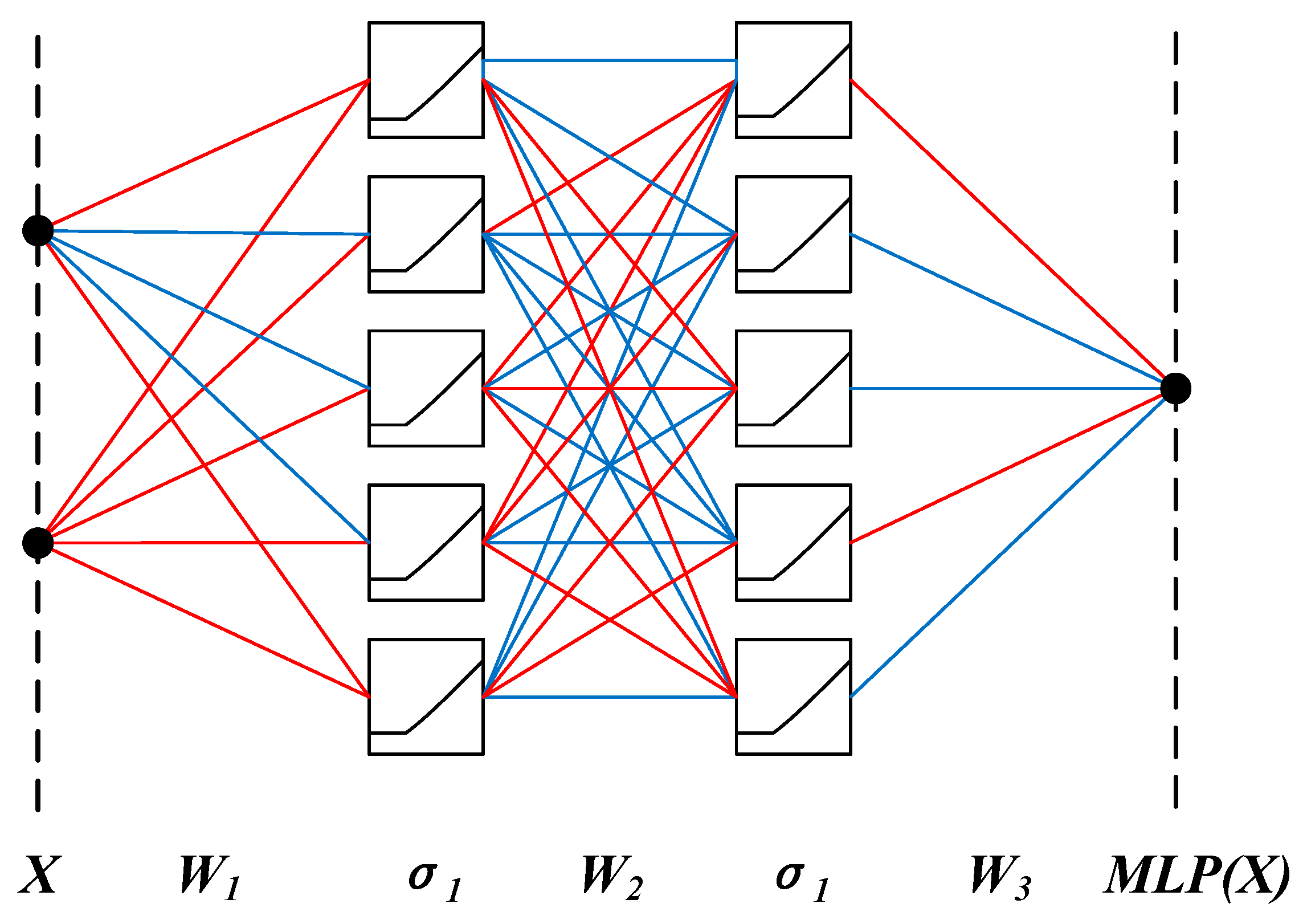
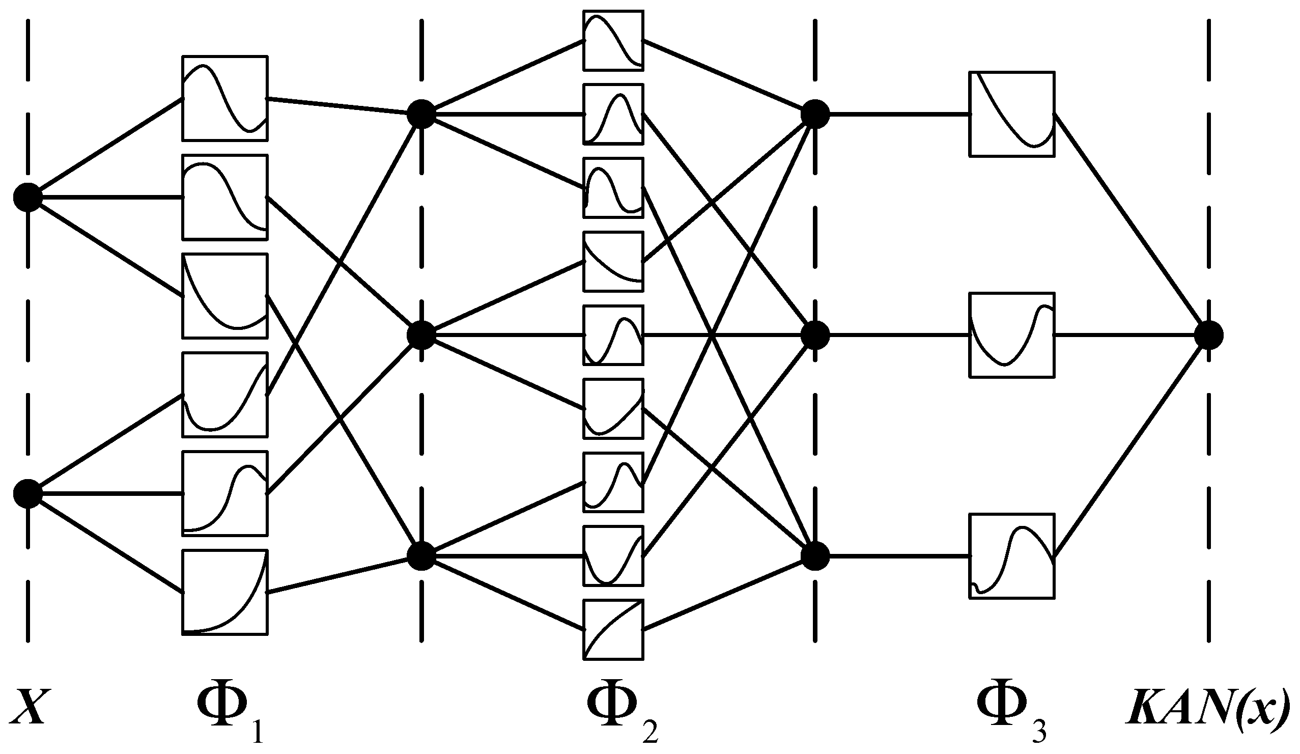
A method for replacing the linear structure of ResNet networks with the nonlinear structure of KAN networks was proposed. The KAN algorithm, an intelligent algorithm proposed by Liu et al. [22] in 2024, is based on the Kolmogorov–Arnold representation theorem. This theorem states that the activation function is no longer a fixed Sigmoid or ReLU; instead, it is learnable and applied to the connection rather than the node. The advantages of the KAN algorithm over the traditional MLP algorithm include achieving higher accuracy with fewer parameters and performing curve learning instead of traditional straight-line learning. The network structures of MLP and KAN are shown in Figure 1 and Figure 2.
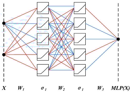
Figure 1.
MLP structure.

Figure 2.
KAN structure.
KAN networks are prone to computational inefficiency and long running times due to the high number of nonlinear structures. This inefficiency arises because the network needs to allocate separate memory space for each activation function to handle intermediate variables during operation. Consequently, the number of stored intermediate variables can be significantly reduced by selecting different basis functions for the inputs to be activated and linearly combining the activation results. Further optimization can be achieved by adjusting the combinations and weights of the different basis functions, as expressed by Equation (3).
KAN Network:
x denotes an input variable and zi is the ith activation function applied to x. For n different activation functions, this implementation requires storing all of the data, resulting in a memory requirement that is linearly proportional to the number of activation functions.
KANS Network:
x denotes an input variable, denotes a set of basis functions, and represents the weight of the corresponding basis functions, where j ranges from 1 to m. To accommodate the above optimization structure, the L1 regularization of the tensor in the original network is replaced by the L1 regularization of the weights, ensuring compatibility between the two. The parameters are initialized using the Kaiming initialization method, which is particularly suitable for handling image recognition tasks in neural networks containing ReLU activation functions.
2.3. Construction of KANS-ResNet-34 Network
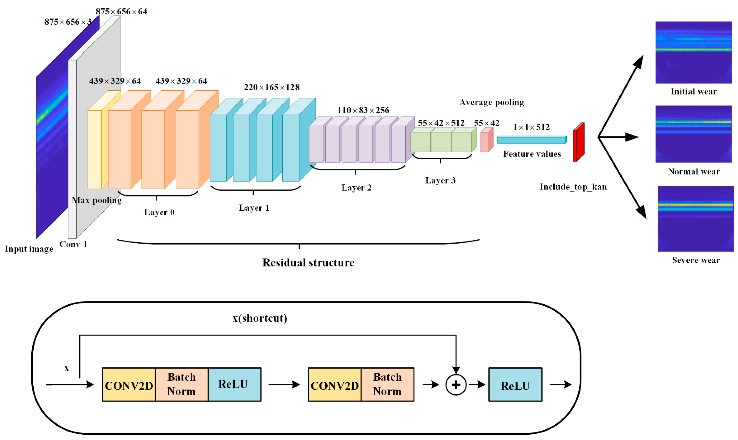
The ResNet-34 network has a simpler structure than the ResNet-50 network; however, its classification accuracy is not high when dealing with complex models. By integrating the classification accuracy of the KANS network with the residual learning approach of ResNet-34, a nonlinear convolutional classifier including _top_kan was used instead of the top linear classifier in the ResNet-34 neural network, as shown in Figure 3. This modification increases the nonlinear structure of the network, enhancing the model’s characterization ability and improving the accuracy of the classification results. Compared with the traditional ResNet-34 network, the KANS-ResNet-34 network has the advantages of fast efficiency, short runtime, and a strong ability to face complex model characterization.

Figure 3.
KANS-ResNet-34 network structure.
The KANS-ResNet-34 network structure is shown in Figure 3, and the specific parameters are listed in Table 1. The construction steps are as follows:

Table 1.
Detailed parameters of three models.
Step I: The raw acquired signals were processed using CWT, converted into CWT time–frequency maps as network inputs, and normalized so that the pixel values satisfied a normal distribution of N(0.5, 0.5).
Step II: The CWT time–frequency map is taken as input in the form of a matrix; 64 convolution kernels with a step size of 2 (Reducing the feature map dimension) and a size of 7 × 7 (Faster capture of large-scale features) are selected with padding = 0. The ReLU function was selected as the activation function, and the basic features of the images were extracted.
Step III: Define two residual blocks: the Basic Block and the Bottleneck Block. The Basic Block contains two 3 × 3 (Progressive construction of more complex feature representations) convolutional layers, each followed by a batch normalization layer and the ReLU activation function. The Bottleneck Block contains three convolutional layers: the first reduces dimensionality with a 1c1 convolutional kernel, the middle performs feature extraction with a 3 × 3 convolutional kernel, and the last, a 1 × 1 convolutional layer, recovers the dimensionality. Each convolutional layer is followed by a batch normalization layer and ReLU activation function.
Step IV: Set up four residual packet structures denoted as Layer [0], Layer [1], Layer [2], and Layer [3], where the four packets contain three, four, six, and three residual blocks, respectively. In the network structure of KANS-ResNet-34, all four residual packet structures of Layer [0], Layer [1], Layer [2], and Layer [3] were connected using a Basic Block.
Step V: The output of Layer [3] is expanded into feature vectors after global average pooling, which is fed into a nonlinear convolutional classifier, including _top_kan, for the classification process. The final output is the three tool wear states.
To evaluate the network performance of the KANS-ResNet-34 network, the ResNet-34 and ResNet-50 networks were introduced for comparison. ResNet-50, with more layers and a more complex architecture than ResNet-34, typically provides better accuracy on large-scale datasets and captures more complex features. However, ResNet-50 requires more computational time and resources, making it less suitable for resource-constrained settings. The construction of both networks follows the steps outlined above, with the key differences being that ResNet-34 uses a fully connected structured linear classifier, while ResNet-50 employs a Bottleneck Block type. The basic parameters of the three networks are listed in Table 1. In Table 1, 3 × 3 and 7 × 7 denote the size of the convolution kernel and 64 denotes the number of that convolution kernel.
3. Milling Cutter Wear Stage Identification Model
3.1. Preprocessing of Signals
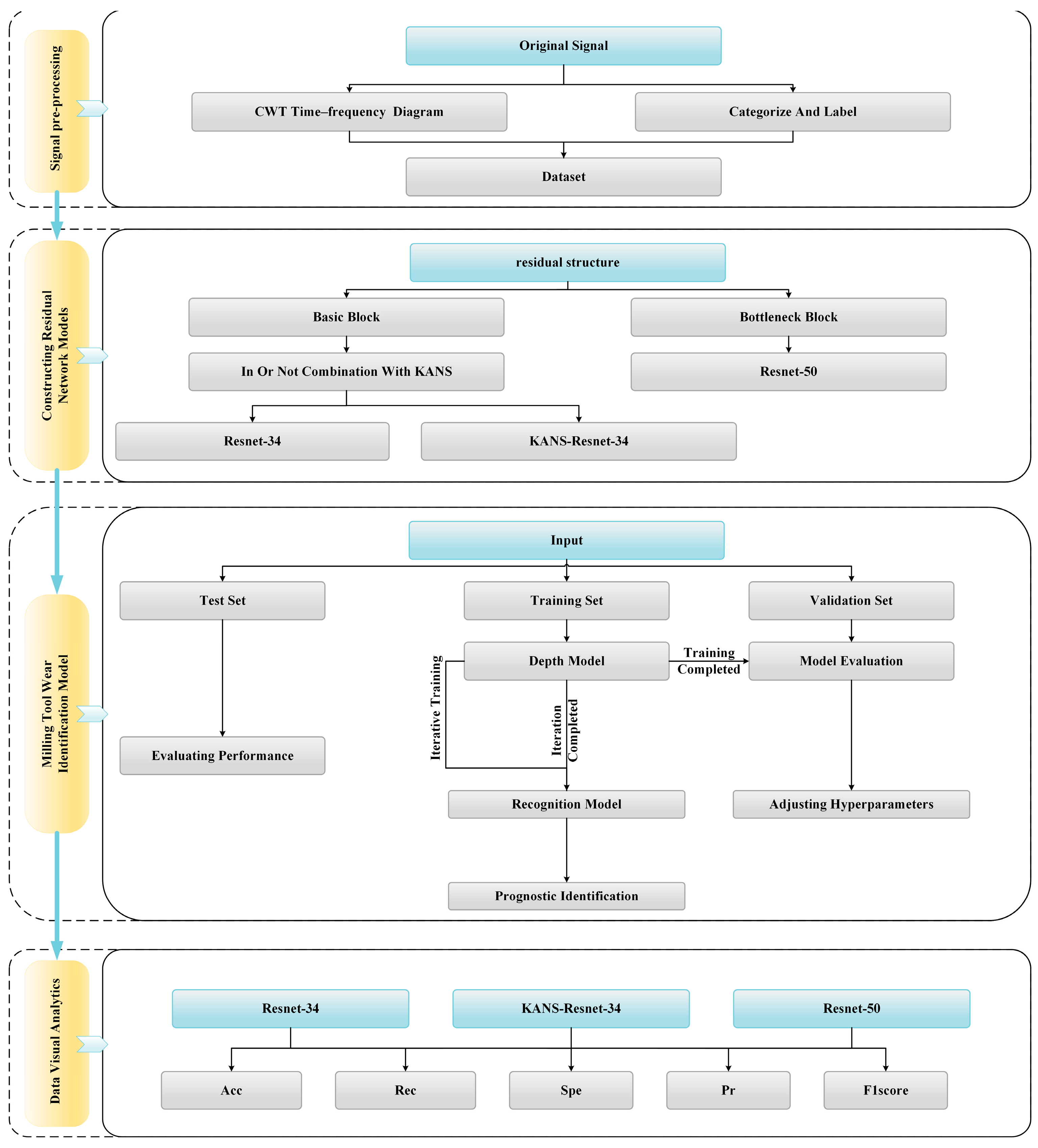
The proposed milling cutter wear stage recognition model consists of three main modules: preprocessing of force, vibration, and acoustic emission signals; feature extraction of each signal; and model training. The force and vibration signals are measured in the x, y, and z directions, allowing for multi-dimensional monitoring of the tool’s status. In this study, the Morlet wavelet was used as the mother wavelet. For the seven-dimensional signals, the wavelet transform, using Formulas (1) and (2), converts the one-dimensional signal features into two-dimensional time–frequency maps. These maps are then used as input to the tool wear state recognition model.
The different colors in the CWT time–frequency diagram represent the corresponding energy distributions at different frequencies and times. A two-dimensional representation of the energy signal is used to replace the original one-dimensional numerical table, allowing for image normalization and preprocessing. By analyzing the value of the wear on the back face (VB) and setting the critical values between initial wear, normal wear, and stable wear, the CWT time–frequency diagrams corresponding to different VB values were manually classified into three categories: initial wear, intermediate wear, and severe wear. The milling cutter wear stage dataset was then constructed based on the classification of the CWT time–frequency diagram features.
3.2. Construction of Residual Network Models
Different deep-learning models were constructed using the Basic and Bottleneck Blocks described in the previous section. ResNet-34 and ResNet-50 utilized the Basic and Bottleneck Blocks, respectively, to combine the classification accuracy of the KANS network with the residual learning approach of the ResNet-34 network, resulting in the KANS-ResNet-34 network. Three residual network models—ResNet-34, KANS-ResNet-34, and ResNet-50—were used as deep learning models for the milling cutter wear stage identification model. All three models consist of four residual packet structures, with reference to the specific model architecture in Table 1. Comparative experiments were conducted to determine which network model offered the best performance.
The dataset, after signal preprocessing as described above, was input into the three models. The same number of iterations, learning rate setting mode, and hyper-parameter settings, such as regularization parameters, were selected for the iterative operation of the models. The classification results were then outputted, and visual verification of the results was carried out.
3.3. Construction of Milling Cutter Wear Recognition Model
To build the training, test, and validation sets, different CWT time–frequency graph feature classifications were coordinated. The training set is the dataset used to train the model, allowing it to adjust its internal parameters (e.g., weights in a neural network) by learning from this set. Validation sets are used for model tuning and selection, helping to determine hyperparameters (e.g., learning rate, number of network layers, number of hidden units) during the training process and to evaluate the model’s performance at different training stages. The test set evaluates the final model’s performance after development is complete. These data were not used during the training and validation process, providing the most realistic feedback on the model’s performance on completely unseen data. In this model construction, using an independent test set of 20% of the total dataset and a training and validation set of 80% of the total dataset, in a ratio of 7:3. The structure of the milling cutter wear recognition model is shown in Figure 4.
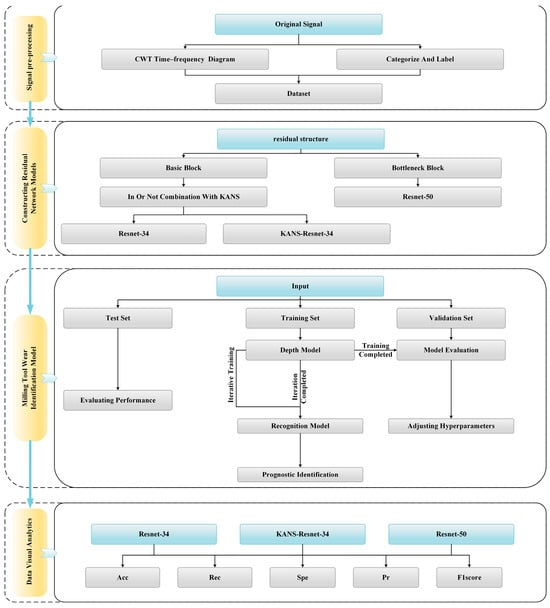
Figure 4.
Milling cutter wear stage identification model.
4. Experimental Verification
4.1. Description of Dataset
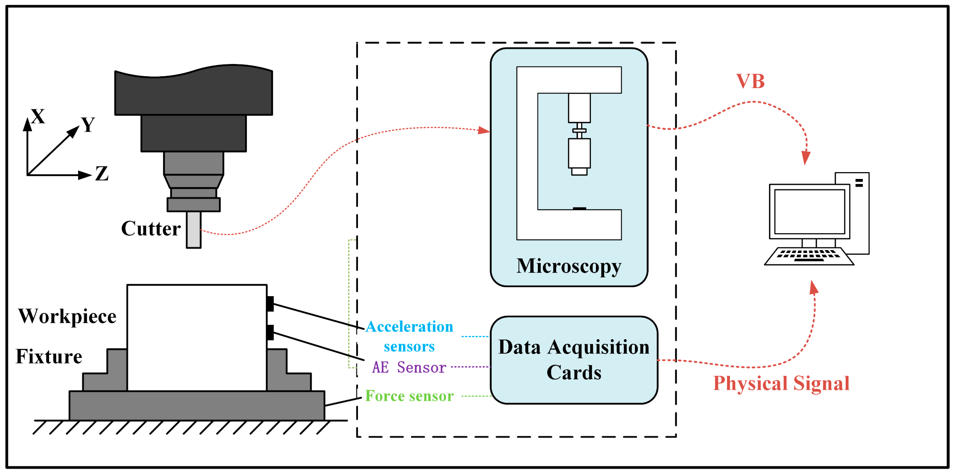
The dataset selected for this study was the PHM Society 2010 dataset, a publicly available dataset used by the American Society for Prediction and Health Management to organize health prediction competitions. The chosen experimental platform was a Röders Tech RFM760 high-speed CNC milling machine (Röders TEC, Soltau, Germany), equipped with a three-flute tungsten carbide ball-end milling cutter, and the workpiece material was stainless steel. The types of signals acquired were force, vibration, and acoustic emission. The force sensor used was a Kistler piezoelectric quartz three-way platform force gauge, the Kistler Model 9257B Dynamic Force Transducer (Kistler Group, Winterthur, Switzerland), which is a highly accurate piezoelectric dynamic force transducer capable of measuring the three orthogonal components of the cutting force (i.e., the force in the X-, Y-, and Z-axis directions). The vibration signal of the machine tool was collected by a piezoelectric acceleration sensor, and the acoustic emission signal was collected by a Kistler acoustic emission sensor. The force and vibration signals were measured in three dimensions (X, Y, and Z), and the acoustic emission signal was one-dimensional data. Thus, the three types of sensors collected a total of seven dimensions of data, measurement of the wear value of the back face using a microscope. The schematic of the tool wear monitoring device is shown in Figure 5.
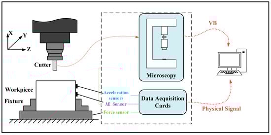
Figure 5.
Schematic of tool wear monitoring device.
This dataset records various signals as well as the average wear value of the back face (VB) for the entire life cycle of six milling cutters. Due to the large amount of data in this dataset and the high-performance requirements of the ResNet-50 network on the computer, this study selects the 1st, 4th, and 6th cutters to save time and balance hardware conditions. Each cutter’s data, after measuring the VB value, was divided into a training set, testing set, and validation set, with a ratio of 7:2:1 for each. The number of milling instances for all three tools was 315, with the end milling material being a square with a length of 108 cm, and each milling instance was equal. The machining parameters used in the test are listed in Table 2. Parameters were chosen for the Society for Prediction and Health Management, New York, NY, USA.
Table 2.
Test parameters.
4.2. Experimental Result
4.2.1. Characterization of Different Signals
According to the PHM dataset’s physical signal categories, the time-domain signal in the CWT time–frequency diagram was used to observe and extract features. Different wear stages of acoustic emission signals, force signals, and vibration signals were selected to characterize the initial wear, normal wear, and severe wear. The wear stages were divided as follows: 1–54 for initial wear, 55–205 for normal wear, and 206–315 for severe wear.
For the force signal, the X-direction of the three wear states in the dataset was selected. The force signal was subjected to CWT transformation, resulting in the CWT time–frequency diagram and the time-domain image shown in Figure 6. In these diagrams, the horizontal axis indicates time, while the vertical axis represents the magnitude of the frequency or the amplitude of the force signal. The different color distributions in the CWT time–frequency diagram represent the distribution of energy. From left to right, the CWT time–frequency diagram and time-domain image correspond to initial wear, normal wear, and severe wear, respectively.
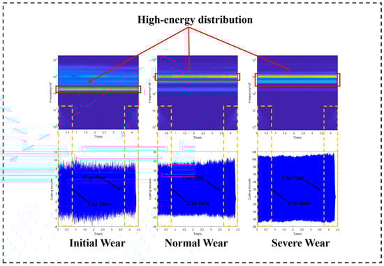
Figure 6.
Analyzing three wear stages of force signals.
As the number of milling passes increased, so did the wear of the milling cutter, resulting in a gradual increase in the axial force. As shown in Figure 6, the high-energy distribution of the force signal is around 102 Hz during the initial wear stage. As wear continues, the high-energy distribution of the force signal gradually shifts to the high-frequency region. In the severe wear stage, the high-energy distribution is mainly concentrated around 103 Hz, and the area of the high-energy region is significantly larger compared to the previous two stages. During tool cut-in and cut-out, the force signals have smaller amplitudes compared to the milling process, but the energy density in the low-frequency part of the CWT frequency map increases, indicating that this process affects the energy distribution in the low-frequency part of the signal. The peak value of the force signal ranges from 8 to 10 N during the initial wear stage, 30–40 N during normal wear, and 100–120 N during the severe wear stage. This indicates a positive correlation between the peak value of the force signal and the wear condition.
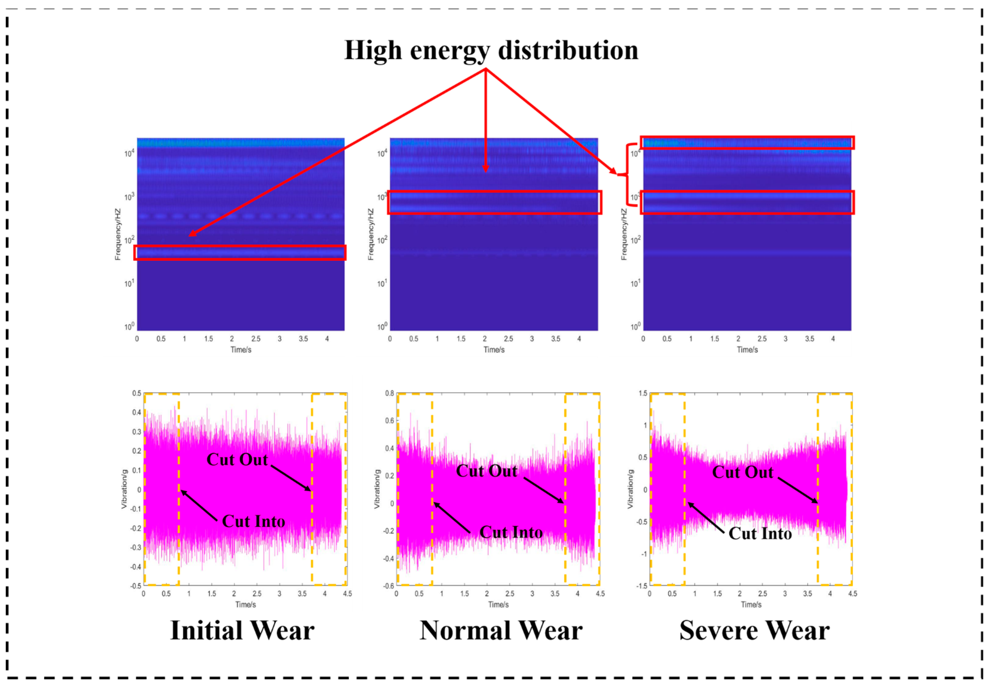
For the vibration signals, the X-direction of the three wear states in the dataset was selected. The same operation as described above was repeated to obtain the CWT time–frequency map and the time-domain image, as shown in Figure 7. As tool wear increases, the milling cutter becomes blunt, resulting in increased vibration during the machining process. Observation of the wavelet scale diagrams for the three wear stages shows that, during initial wear, the high-energy distribution of the vibration signal is around 102 Hz. As wear worsens, the high-energy distribution of the vibration signal extends to the high-frequency region, with a significantly larger high-energy distribution area. During tool cut-in and cut-out, the vibration signals are larger compared to the milling process. However, the CWT time–frequency plots show no significant difference, indicating that this process affects the vibration amplitude without significantly affecting the signal energy distribution. The peak value of the vibration signal follows the same trend as that of the force signal, gradually increasing with the intensification of the wear condition, demonstrating a positive correlation.

Figure 7.
Analyzing three wear stages of vibration signals.
For the acoustic emission signal, the three wear states in the dataset were selected. The same operation as described above was repeated to obtain the CWT time–frequency map and the time-domain image, as shown in Figure 8. As the tool wear condition worsens, cutting force and vibration increase, leading to greater energy release during material deformation and fracture. This results in an enhancement of the high-energy amplitude of the acoustic emission signal and an increase in the energy density at the high-energy distribution in the CWT time–frequency diagram. The acoustic emission signal is larger during tool cut-in and cut-out than during milling, with a significant increase in the energy density of the CWT time–frequency map. This indicates that these processes affect the acoustic emission amplitude and increase the energy share of the low-frequency part. As the wear condition increases, the elastic waves released by the destruction of the tool and workpiece material increase, causing the amplitude of the acoustic emission signal to become larger.
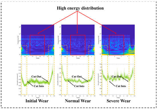
Figure 8.
Analyzing three wear stages of AE signals.
The analysis above shows that the CWT time–frequency diagrams of force signals, vibration signals, and acoustic emission signals exhibit obvious differences in energy intensity distribution at different wear stages. The time and frequency bands also differ, indicating the feasibility of using two-dimensional CWT time–frequency diagrams instead of the one-dimensional original physical signals. Therefore, CWT time–frequency diagrams of the various types of signals can be effectively used as inputs to the model.
4.2.2. Results and Analysis
In this study, three sets of comparative tests of the models—KANS-ResNet-34, ResNet-34, and ResNet-50—were conducted. The classification ability of the constructed models served as the evaluation criterion for the tool wear state recognition system. To assess the advantages and disadvantages of the new model constructed in this study compared to the two original models, the classification ability was evaluated using the test set from the experiment. The model performance was evaluated using the following five classification metrics: accuracy, sensitivity, specificity, checking accuracy, and F1 score, which are expressed by the following formulas:
Accuracy:
Recall Ratio:
Specificity:
Precision:
F1 Score:
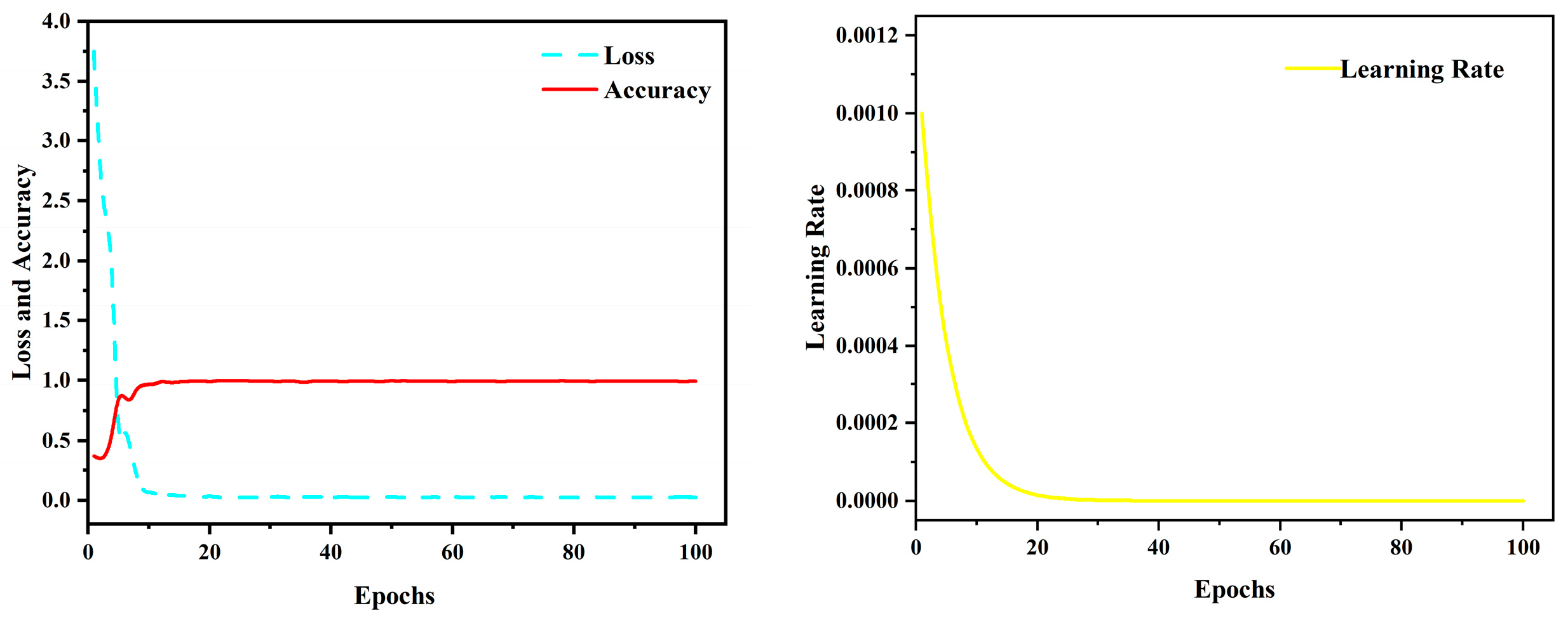
where true positive (TP) is the number of samples in which the actual wear state matches the predicted wear state, false positive (FP) is the number of samples in which another wear state is incorrectly predicted as that wear state, true negative (TN) is the number of samples in which other wear states are correctly predicted to not belong to that category, and false negative (FN) is the number of samples that were actually in that wear state but were predicted incorrectly. In multi-categorization tasks, the concepts of true-positive (TP) and true-negative (TN) examples are slightly different from those in binary categorization and need to be subdivided for each category. We usually compute these metrics by treating each category as a separate binary classification problem, and the categorization results used in this manuscript are computed for the categorization results in the network output confusion matrix for the macro concept. The KANS-ResNet-34 model is selected, with an epoch set to 100 iterations, and the improved adaptive learning rate algorithm AdamW is chosen. AdamW, an optimization algorithm based on Adam, improves weight decay, making it more effective in handling regularization and better at avoiding overfitting. The resulting accuracy, loss, and learning rate curves are shown in Figure 9.
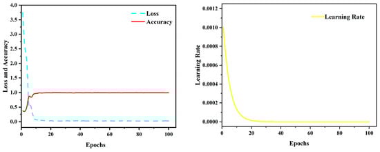
Figure 9.
Accuracy, loss, and learning rate curves for epochs = 100.
Figure 9 shows that when the epoch number of the KANS-ResNet-34 model reaches 30, the accuracy and loss of both the training and validation sets stabilize and reach a high level. This indicates that the model has achieved convergence, and the learning rate gradually stabilizes at this point. To avoid unnecessary iterative operations and the risk of “pseudo-convergence,” the early stopping method is used to select the optimal model. At this point, the model’s accuracy reaches 99.37%, with the epoch set to 50 for the entire test, making 50 the number of iterations.
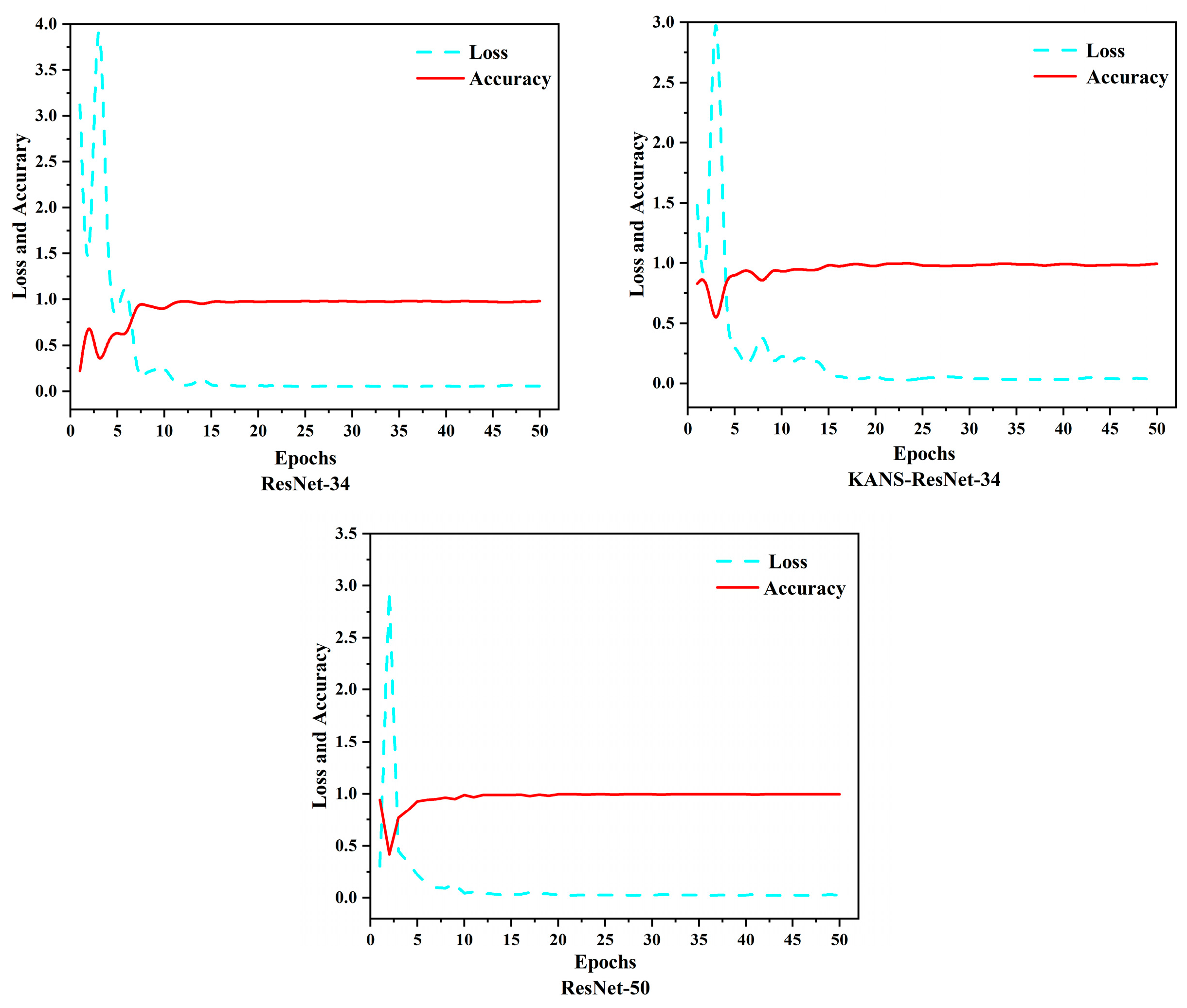
KANS-ResNet-34, ResNet-34, and ResNet-50 were trained and tested with an epoch of 50. The accuracy and loss of the three models are shown in Figure 10.
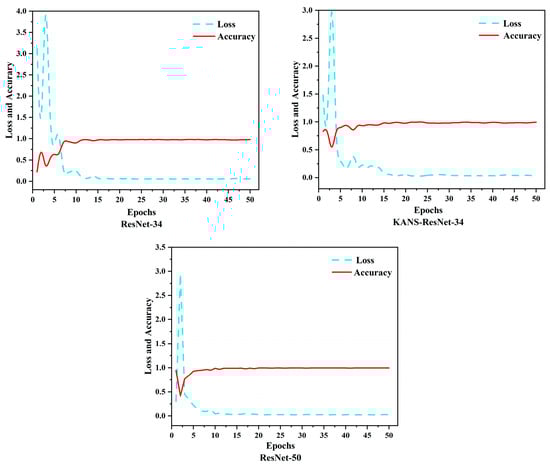
Figure 10.
Loss and accuracy plots for three models.
As shown in Figure 10, the accuracy and loss of all three models stabilized with an increase in the number of iterations, with the most variation occurring in the first five iterations. The KANS-ResNet-34 and ResNet-50 models stabilized around 10 iterations, whereas the ResNet-34 model stabilized only around 15 iterations. The KANS-ResNet-34 and ResNet-50 models both exhibited smaller loss fluctuations compared to the ResNet-34 model. The KANS-ResNet-34 model reached a maximum accuracy of 99.28% at 15 iterations, while the ResNet-50 model achieved a maximum accuracy of 99.64% at 20 iterations. The ResNet-34 model, although achieving its highest accuracy at 20 iterations, had a maximum accuracy of 98.21%, which was slightly lower than that of the other models. During the iterative runs, the KANS-ResNet-34 and ResNet-34 models required a similar amount of time, with 50 iterations taking approximately 1 h. In contrast, the ResNet-50 model took approximately 33.3 h for 50 iterations. The accuracy of KANS-ResNet-34, proposed in this paper, is about 1.07% higher than that of the original ResNet-34 model. Although it is 0.36% lower than that of the ResNet-50 model, the running time of ResNet-50 at the same number of iterations is 33.68 times longer than that of KANS-ResNet-34. Considering that both models have an accuracy of more than 99%, the economy and feasibility of the KANS-ResNet-34 model are significantly better than those of ResNet-50. Therefore, the KANS-ResNet-34 model outperformed the other two models.
To further analyze the classification prediction ability of the KANS-ResNet-34 model proposed in this paper, data visualization and analysis were performed using a test set. All the samples in the test set for the initial and severe wear stages were predicted accurately, while four samples in the normal wear stage were incorrectly predicted to be in the severe wear stage. The accuracy of the prediction in the initial and severe wear stages was 100%, the accuracy of the prediction in the normal wear stage was 95.12%, and the accuracy for the overall samples was 97.79%. The prediction results of the test set are shown in Figure 11.
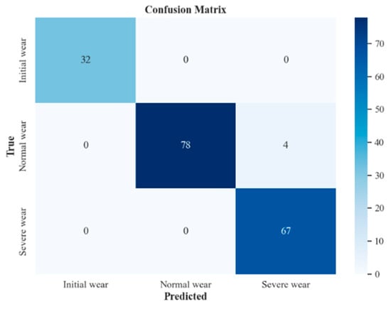
Figure 11.
KANS-ResNet-34 model prediction results.
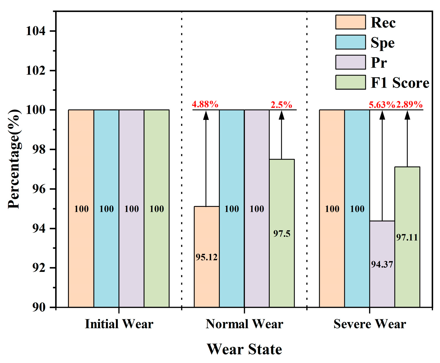
To accurately assess the comprehensive performance of the proposed deep learning model, other evaluation parameters of the model were calculated, as shown in Figure 12 and Table 3.
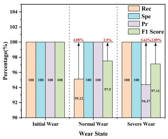
Figure 12.
KANS-ResNet-34 model performance analysis.
Table 3.
KANS-ResNet-34 model performance analysis.
From Table 3, it can be seen that the model has the best performance in specificity (Spe), which is 100% for all three categories, representing the model’s ability to classify consistently across all categories. The model’s recall (Rec) is 100% for the initial and severe wear phases, indicating that the model is extremely sensitive to data from these two phases. The slightly lower recall for the normal wear phase may be due to the larger number of intermediate samples. The precision (Pr) of the model is also 100% for the initial and normal wear phases, indicating 0% misidentification in these two phases, while the lower precision in the severe wear phase is due to misidentifying four samples from the normal wear phase as being in the severe wear phase. The model’s performance on the F1 scores for the three categories is superior, all above 95%, with the best F1 score even reaching 100%. This indicates that the model’s overall classification performance is well-balanced and has the ability to handle large-scale and complex data. Similar conclusions can be seen in Table 4 and Table 5, where the recall for the normal wear phase is still slightly lower at 93.90% in Table 4, compared to 97.56% in Table 5, and the F1 scores for both are 96.85% and 98.76%, respectively, and the ResNet-34 model has lower values for each of the values in the normal wear phase than the KANS-ResNet-34 model, whereas the KANS-ResNet-34 model is very close to the ResNet-50 model for all values. For the severe wear stage, the three models have the same trend as the normal wear stage. The F1 scores of the three models are ResNet-50, KANS-ResNet-34, and ResNet-34 in descending order, and the optimized KANS-ResNet-34 model is superior in terms of the F1 scores and the cost of time used by the three models in the previous section and is well suited for tool wear monitoring.
Table 4.
ResNet-34 model performance analysis.
Table 5.
ResNet-50 model performance analysis.
5. Conclusions
In this study, we addressed the challenging problem of tool state monitoring for milling cutters during machining and production by proposing a change in the deep learning model classifier. This method effectively improved the accuracy of tool wear state monitoring while allowing the use of a shallow network model instead of a deep network model, thereby reducing the model’s complexity and ensuring classification accuracy. The conclusions are as follows:
- (1)
- After transforming the original physical signals into CWT time–frequency diagrams using a continuous wavelet transform, the CWT time–frequency diagrams corresponding to each stage of wear and tear exhibited obvious differences. As the degree of wear and tear increased, the signal amplitude of the three types of signals increased, resulting in more energy being contained in the signal. This energy gradually shifted to the high-frequency portion of the signal, which was converted into a form of a picture that accurately described the signal’s local details of the time–frequency information, making it more suitable as an input to the classification network.
- (2)
- Optimizing the KAN by activating the inputs using different basis functions and then combining them linearly reduced the computational cost of the computer and significantly improved efficiency. To accommodate this optimized structure, the L1 regularization of the tensor in the original network was replaced by the L1 regularization of the weights, making the two compatible. Additionally, the parameters were initialized using the Kaiming initialization method.
- (3)
- Using the nonlinear structure of the KANS network, the include_top_kan nonlinear classifier was constructed to replace the top linear classifier in the ResNet-34 neural network. Experiments conducted on the ResNet-34 and ResNet-50 models demonstrated the feasibility of replacing the deep network model with a shallow network model, substantially saving time and guaranteeing classification accuracy. The accuracy of the KANS-ResNet-34 model reached 99.28% in the validation set and 97.79% in the test set.
Author Contributions
Conceptualization, B.C. and Y.Z.; methodology, B.C.; software, Y.Z.; validation, B.C., Y.Z., and B.L.; formal analysis, B.C.; investigation, Y.Z.; resources, Y.Z.; data curation, C.P.; writing—original draft preparation, B.C.; writing—review and editing, Y.Z.; visualization, B.L.; supervision, Y.Z.; project administration, B.L.; funding acquisition, Y.Z. All authors have read and agreed to the published version of the manuscript.
Funding
This study was supported by the National Natural Science Commission of China—Mechanism of damage generation and key technology of high quality hole making for aerospace heterogeneous components (Grant No. 51875367) and Liaoning Provincial Department of Science and Technology—Stress detection standard for the whole process of aluminum alloy thin-walled parts manufacturing and collaborative control technology of machining and assembly deformation (Grant No. 2022JH2/101300213).
Institutional Review Board Statement
Not applicable.
Informed Consent Statement
Not applicable.
Data Availability Statement
The raw data supporting the conclusions of this article will be made available by the authors on request.
Conflicts of Interest
Authors Bengang Liu and Chunyang Peng were employed by the company Shenyang Aircraft Company. The remaining authors declare that the re-search was conducted in the absence of any commercial or financial relationships that could be construed as a potential conflict of interest.
References
- Cheng, Y.N.; Gai, X.Y.; Guan, R.; Jin, Y.B.; Lu, M.D.; Ding, Y. Tool wear intelligent monitoring techniques in cutting: A review. J. Mech. Sci. Technol. 2023, 37, 289–303. [Google Scholar] [CrossRef]
- Huang, W.Z.; Li, Y.; Wu, X.; Shen, J.N. The wear detection of mill-grinding tool based on acoustic emission sensor. Int. J. Adv. Manuf. Technol. 2023, 124, 4121–4130. [Google Scholar] [CrossRef]
- Panda, A.; Nahornyi, V.; Valíček, J.; Harničárová, M.; Kušnerová, M.; Baron, P.; Pandová, I.; Soročin, P. A novel method for online monitoring of surface quality and predicting tool wear conditions in machining of materials. Int. J. Adv. Manuf. Technol. 2022, 123, 3599–3612. [Google Scholar] [CrossRef]
- Lu, Z.; Wang, M.; Dai, W. Machined surface quality monitoring using a wireless sensory tool holder in the machining process. Sensors 2019, 19, 1847. [Google Scholar] [CrossRef]
- Wang, C.; Bao, Z.; Zhang, P.; Ming, W.; Chen, M. Tool wear evaluation under minimum quantity lubrication by clustering energy of acoustic emission burst signals. Measurement 2019, 138, 256–265. [Google Scholar] [CrossRef]
- Kong, D.; Chen, Y.; Li, N.; Duan, C.; Lu, L.; Chen, D. Tool wear estimation in end milling of titanium alloy using NPE and a novel WOA-SVM model. IEEE Trans. Instrum. Meas. 2019, 69, 5219–5232. [Google Scholar] [CrossRef]
- Pu, X.; Jia, L.; Shang, K.; Chen, L.; Yang, T.; Chen, L.; Gao, L.; Qian, L. A new strategy for disc cutter wear status perception using vibration detection and machine learning. Sensors 2022, 22, 6686. [Google Scholar] [CrossRef]
- Kim, G.; Yang, S.; Kim, D.; Kim, S.; Choi, J.; Ku, M.; Lim, S.; Park, H. Bayesian-based uncertainty-aware tool-wear prediction model in end-milling process of titanium alloy. Appl. Soft Comput. 2023, 148, 110922. [Google Scholar] [CrossRef]
- Niu, B.; Sun, J.; Yang, B. Multisensory based tool wear monitoring for practical applications in milling of titanium alloy. Mater. Today Proc. 2020, 22, 1209–1217. [Google Scholar] [CrossRef]
- Serin, G.; Sener, B.; Ozbayoglu, A.M.; Unver, H.O. Review of tool condition monitoring in machining and opportunities for deep learning. Int. J. Adv. Manuf. Technol. 2020, 109, 953–974. [Google Scholar] [CrossRef]
- Bagga, P.; Makhesana, M.; Patel, H.; Patel, K. Indirect method of tool wear measurement and prediction using ANN network in machining process. Mater. Today Proc. 2021, 44, 1549–1554. [Google Scholar] [CrossRef]
- Chen, L.; Li, S.; Bai, Q.; Yang, J.; Jiang, S.; Miao, Y. Review of image classification algorithms based on convolutional neural networks. Remote Sens. 2021, 13, 4712. [Google Scholar] [CrossRef]
- Zhao, J.; Guo, S.; Ma, L.; Kong, H.; Zhang, N. Tool wear monitoring based on an improved convolutional neural network. J. Mech. Sci. Technol. 2023, 37, 1949–1958. [Google Scholar] [CrossRef]
- Lin, X.; Chao, S.; Yan, D.; Guo, L.; Liu, Y.; Li, L. Multi-Sensor Data Fusion Method Based on Self-Attention Mechanism. Appl. Sci. 2023, 13, 11992. [Google Scholar] [CrossRef]
- He, K.; Zhang, X.; Ren, S.; Sun, J. Deep residual learning for image recognition. In Proceedings of the IEEE Conference on Computer Vision and Pattern Recognition, Las Vegas, NV, USA, 27–30 June 2016; pp. 770–778. [Google Scholar]
- Guan, Z.; Wang, F.; Wang, G.; Zheng, H. Improved depth residual network based tool wear prediction for cavity milling process. Int. J. Adv. Manuf. Technol. 2024, 130, 1759–1777. [Google Scholar] [CrossRef]
- Zhou, J.; Yue, C.; Liu, X.; Xia, W.; Wei, X.; Qu, J.; Liang, S.; Wang, L. Classification of tool wear state based on dual attention mechanism network. Robot. Comput. -Integr. Manuf. 2023, 83, 102575. [Google Scholar] [CrossRef]
- Jiang, Z.; Wang, F.; Mou, W.; Zhu, S.; Fu, R.; Yu, Z. Method for edge chipping monitoring based on vibration polar coordinate image feature analysis. Int. J. Adv. Manuf. Technol. 2024, 130, 5137–5146. [Google Scholar] [CrossRef]
- Zhang, Y.; Qi, X.; Wang, T.; He, Y. Tool wear condition monitoring method based on deep learning with force signals. Sensors 2023, 23, 4595. [Google Scholar] [CrossRef]
- Zhang, B.; Liu, X.; Yue, C.; Liu, S.; Li, X.; Liang, S.Y.; Wang, L. An imbalanced data learning approach for tool wear monitoring based on data augmentation. J. Intell. Manuf. 2023, 35, 1–22. [Google Scholar] [CrossRef]
- Lee, J.; Kwak, K. Heart Sound Classification Using Wavelet Analysis Approaches and Ensemble of Deep Learning Models. Appl. Sci. 2023, 13, 11942. [Google Scholar] [CrossRef]
- Liu, Z.; Wang, Y.; Vaidya, S.; Ruehle, F.; Halverson, J.; Soljačić, M.; Hou, T.Y.; Tegmark, M. Kan: Kolmogorov-arnold networks. arXiv 2024, arXiv:2404.19756. [Google Scholar]


Disclaimer/Publisher’s Note: The statements, opinions and data contained in all publications are solely those of the individual author(s) and contributor(s) and not of MDPI and/or the editor(s). MDPI and/or the editor(s) disclaim responsibility for any injury to people or property resulting from any ideas, methods, instructions or products referred to in the content. |
© 2024 by the authors. Licensee MDPI, Basel, Switzerland. This article is an open access article distributed under the terms and conditions of the Creative Commons Attribution (CC BY) license (https://creativecommons.org/licenses/by/4.0/).