A Novel Approach of the Viscoelasticity of Axially Functional Graded Bar and Application of Harmonic Vibration Analysis of an Isotropic Beam as Support

Abstract

The use of smart materials and passive controllers in modern technologies has stimulated the study of vibration in elastic systems with viscoelastic damping. It is also possible to create components with precise material distribution coefficients and distinct properties, such as Functionally Graded Materials. This work investigates the resonant frequency characteristics of a beam supported at its ends by Axially Functionally Graded (AFG) viscoelastic bars using the finite element method. The set of equations governing motion is obtained by assuming Euler–Bernoulli beam theory for the beam and bar theory for the bars using Lagrange’s equations. The material properties of the functionally graded bar is assumed to vary through the length according to the power law distribution. The longitudinal loss factor values are used to define the internal damping coefficient, which is also dependent on the Young’s modulus value varying along the bar. The effects of the length-varying material properties and internal damping of the FG support bars on the force transmission T_R and frequency parameters λ are examined in detail. No study has been found in the literature on the vibration of viscoelastic FG bar-supported beams subjected to a harmonic force at the centre point. It is shown that using bars formed with combinations of different materials considering material damping will be useful to keep the vibration level and force transmission at a certain value and control the frequency parameters.

1. Introduction

Beams are important structural elements both alone or as system elements. Their dynamic conditions have especially been the subject of study for many researchers. The boundary conditions and their damping properties affecting the dynamic state are significant in vibration assessment [1,2,3,4,5]. Damping has an important place in the vibration analyses of beam and plate elements that form the basis of engineering applications. Many mathematical models are utilised in the damped vibration analysis of continuous systems to represent the dissipation and damping mechanisms. Mathematical models that characterise the mechanical characteristics of materials are an ongoing topic in engineering study. Due to their linearity, the Kelvin–Voigt and Maxwell models are simpler and more suitable for modelling. Damping applications in boundary supports are an alternative to surface damping applications using viscoelastic materials. Although the damping effect is obtained by the layer effect on the surface in practice, it is also very common to apply it as a boundary condition [1,2,3]. Fan et al. [1] used a complex normal mode analysis approach to study the forced vibration of a beam with viscoelastic boundary supports. The viscoelastic support regions were defined in terms of equivalent complex stiffness coefficients. They separated the equations of motion using complex modes with complex stiffness and investigated the impact of viscoelastic supports on forced vibration response. The Young’s modulus of the viscoelastic material is a complex number that consist of E_r, the storage modulus and η, the loss factor of the material. In addition to the investigation of the vibration characteristics of the beam with viscoelastic boundary conditions, the response of the beam under various boundary conditions has been the focus of interest for researchers [3,4]. Studies have been carried out according to the characteristics of the external force. The damping effect was investigated by applying the force randomly and harmonically from the centre or end points of the beam [2,3,4,5]. The addition of mass and damping elements to the beam and the effects of their locations on the vibration response have been the subject of research on the optimum vibration values [5,6]. Wang and Wen [4] conducted a study to determine the best position for viscoelastic supports in reducing vibration levels in a beam that is exposed to harmonic force. Their analysis was based on the Rayleigh damping model, which combines stiffness and mass matrices.

Damping has a complicated and unpredictable nature. The dissipating energy is a physical phenomenon and arises via damping in vibrating systems. Considering velocity, displacement and strain parameters, the researchers tried to model the viscoelasticity and dissipation behaviour of solid metallic material. Studies are carried out for hysteretic and viscous damping and equivalent damping in the literature. Viscous and hysteretic damping models are linear damping models. Hysteresis losses in materials due to slippage between micro-surfaces cause damping in typical structures without considering specific viscous, Coulomb and viscoelastic damping elements. It is common to consider viscous damping as either proportional or Rayleigh-type. This is a result of the damping matrix being capable of diagonalization using the same real eigenvectors employed to diagonalize the mass and stiffness matrices [7,8,9,10]. He and Fu [9] described structural damping with two real positive constants like the proportional viscous damping case. Therefore, the damping matrix [H] can be written proportional to the stiffness [K] and mass [M] matrices ([H] = ν[K] + μ[M]). Each mode has its damping loss factor for a system with proportional structural damping. ν and μ are damping constants. When μ = 0, the damping matrix only depends on the stiffness matrix, meaning the damping loss factor for all modes is constant ν. For the nonproportional structural damping, the imaginary part of a complex stiffness matrix [K]_c can be defined with the structural damping matrix [H] [9].

The magnitude of energy loss depends upon material type and modes of vibration. Experiments demonstrate that the energy loss per cycle due to internal friction is independent on frequency but is roughly related to the square of amplitude. The structural damping constant is acceptable for forced harmonic motion. So, the dynamic analysis of the bar with viscoelastic material is performed with the complex modulus in the frequency domain [11]. Maia [12] suggested a solution using the constant hysteretic damping model for the free vibration response problem. Structural damping always dissipates energy from the system. The loss coefficient η equals the ratio of specific damping capacity per radian to the strain energy. Lisitano et al. [13] presented a material-specific damping parameter based on the Bernoulli–Euler beam theory as an addition to the proportional damping approach. The modal damping ratio of each mode was calculated using the material damping coefficient. They assumed that the damping energy is proportional to the local modal strain energy. The results were validated experimentally. The authors proposed a material-specific damping parameter that enables the calculation of structure-specific damping parameters based on theoretical or numerical mode forms. Hysterical damping is generally significant for steady-state vibrations, but there are studies for other forms of forced vibrations. Pan et al. [14] proposed a new approach to overcome the instability of the solution. In addition to the real boundary conditions, by creating virtual boundary conditions, they eliminated divergence terms of the complementary solution for the direct integration solution and converged to the exact solution.

The following studies are available if we consider the internal viscous damping approaches in a general framework. The developed formulation of variable damping along the bar is based on this approach in the study. Tsai et al. [15] analysed the vibration of a Timoshenko beam with partially and fully distributed internal viscous damping. They showed that the natural frequencies decreased with increasing damping, with internal damping fully distributed. Locally distributed internal damping was more effective when the damped segment was at the position with the maximum bending moment. The dissipation function of the beam was written considering the directional velocity, rotational velocity, bending and shearing internal damping coefficients. Chen [16] studied the vibration of the axially loaded Timoshenko beam with locally distributed internal damping of Kelvin–Voigt type. The Eigen frequencies of the damped beams were determined. The effects of the internal damping considering sizes and location parameters on the damped natural frequency were investigated. Kocaturk and Simsek [17] studied the vibration of a viscoelastic beam under the consideration of the Euler–Bernoulli beam theory. For the viscoelasticity of the beam, the Kelvin–Voigt model was used. The damping of the beam is assumed to be proportional to the mass and stiffness of the beam as internal. Abu-Hilal and Mohsen [3] investigated the vibrations of the beam exposed to the moving harmonic load for the general boundary conditions. For the material, the Kelvin–Voigt model was used. The dissipation function of the beam was written in the form of internal damping of the beam and proportionality constant. Freundlich [18] studied the transient vibration of the Bernoulli–Euler cantilever beam under base motion with a rigid mass attached at the end. A fractional Kelvin–Voigt model is used to describe the viscoelastic properties of the beam material. A method of calculating the damped natural frequencies of the beam was introduced. He derived the solution for the forced vibration of the beam by using the mode superposition method. Chen [19] analysed the bending vibration of an axially loaded twisted beam with locally distributed internal damping of the Kelvin–Voigt type. They used Timoshenko’s beam theory and Hamilton’s principle. The Eigen frequencies are studied concerning the internal damping, the sizes and positions of the damped segment, twist angle and the axial load. He showed how different damped beam parameters affect the vibration characteristics of the beam.

Due to the integration of smart materials and passive controllers in present-day technologies, the research on vibration in elastic systems with viscoelastic damping has increased. It is also possible to manufacture components with specific material distribution coefficients and different properties like Functionally Graded Materials (FGM). This allows combining solidness, thermal conductivity and friction in exact proportions. The transition between different materials through the thickness or length of the beam can be described as an exponential or sigmoid function. This change is only taken into account in the direction of thickness or length, or thickness and length (bi-directional functionally graded material, BDFGM). Generally, material properties are considered as varying along the thickness direction in the studies on FGM beams. Despite the constraints of the manufacturing process, researchers are highly interested in this technology because of its numerous benefits. However, despite the extensive research on beams and plates, little has been conducted on beams and plates that are supported by springs and dampers, considering their viscoelastic properties. Furthermore, as far as I am aware, the dynamic response characteristics of a beam supported by axially FG viscoelastic bars have not been investigated yet.

In the studies of beams with Functionally Graded Materials, the damping was applied discretely or defined as the material damping for the FGM beam. Sepehri et al. [20] explored the vibration response of beams made of functionally graded (FG) and viscoelastic materials installed on the Pasternak foundation in their study. They aimed to investigate the effectiveness of vibration suppression in a simply supported FG beam subjected to a point harmonic load. They introduced fractionally damped absorbers to reduce the beam deflection at natural frequencies to achieve this. A new method was developed to obtain analytical solutions using Laplace transformations. Demir and Oz [21] utilised the finite element method to investigate the resonance frequency response of a beam using the Euler–Bernoulli beam theory with functionally graded material under viscoelastic boundary conditions. The material characteristics of the beam varied with thickness according to a power law distribution. Different stiffness and damping coefficients are employed in viscoelastic support components to achieve various boundary conditions. Deng et al. [22] conducted a study on the dynamic stiffness matrix of a double-functionally graded Timoshenko beam system on Winkler–Pasternak under axial stress. They also took into account the damping of the connecting layer. The research compared the effect of gradient parameters, foundation parameters, axial loading and connection stiffness on the frequency and buckling load. Furthermore, they studied the effects of the damping factor on the system. FG beam with an elastic foundation and spring supports was investigated by Duy et al. [23] for its free vibration response. The exponential law dictated that Young’s modulus, mass density and beam width should vary in thickness and axial direction. Akbas et al. [24] conducted a study on the vibration response of a thick beam made of functionally graded porous material subjected to a dynamic sine pulse load with damping effects. They used an accepted finite element model and incorporated the damping effect into the model using the Kelvin–Voigt viscoelastic constitutive model. The study investigated the impact of layer stacking sequence, material gradation index and porosity parameter on the dynamic response of the beam. The researchers used the Kelvin–Voigt material model due to its linearity. η is the damping ratio defined as the ratio of the damping constant to Young’s module. The damping ratio is selected as η = 0.0001 to represent the damping matrix [C] as follows. [C] = η[K], where [K] is the stiffness matrix.

The transition between different materials through the length of the bar can be described as an exponential function. The axial bar approach is used for the system elements that are subjected to a coercive force in the axial direction. Therefore, the axial bar theory is used in the formulations with the assumption that the displacements in the direction of other axes are small [25,26,27]. Vibration damping studies using axial FG bars are more recent and very few in number. Mi and Song [28] designed a beam with an Axially Functionally Graded design, considering the deflection mode. They used the material properties and geometric parameters to realise the vibration control of specific regions on the beam structures. Demir [29] considered an Axially Functionally Graded (AFG) bar as a support element. He investigated the frequency parameters of the AFG bar for the viscoelastic and point mass boundary conditions. He interpreted the structural behaviour of the AFG bar for the power law exponent n.

The vibration isolation and the force transmitted to the ground have been considered in the context of isotropic and FG beams in the literature. These studies used internal material damping and discrete damping elements for vibration suppression. In this study, internal damping coefficients are defined by using material longitudinal damping values and Young’s moduli from the literature. A functionally graded material approach is used to formulate the exponential variation of the internal damping coefficients between the two ends of the bar. This approach is based on the dissipation behaviour of solid metallic material losses due to slippage between micro-surfaces. Bars with varying materials and internal damping properties in the axial direction are attached to the beam at the ends under the effect of harmonic force. It is impossible to minimise both the vibration displacements and the force transmitted to the ground. Either the vibration amplitudes or the force transmitted to the ground remain large. Smaller displacements can be achieved with such structures according to spring support. By controlling the material and damping distribution, it will be possible to provide the desired frequency value and isolation. When we evaluate the system as application areas, the following observations are made:

-

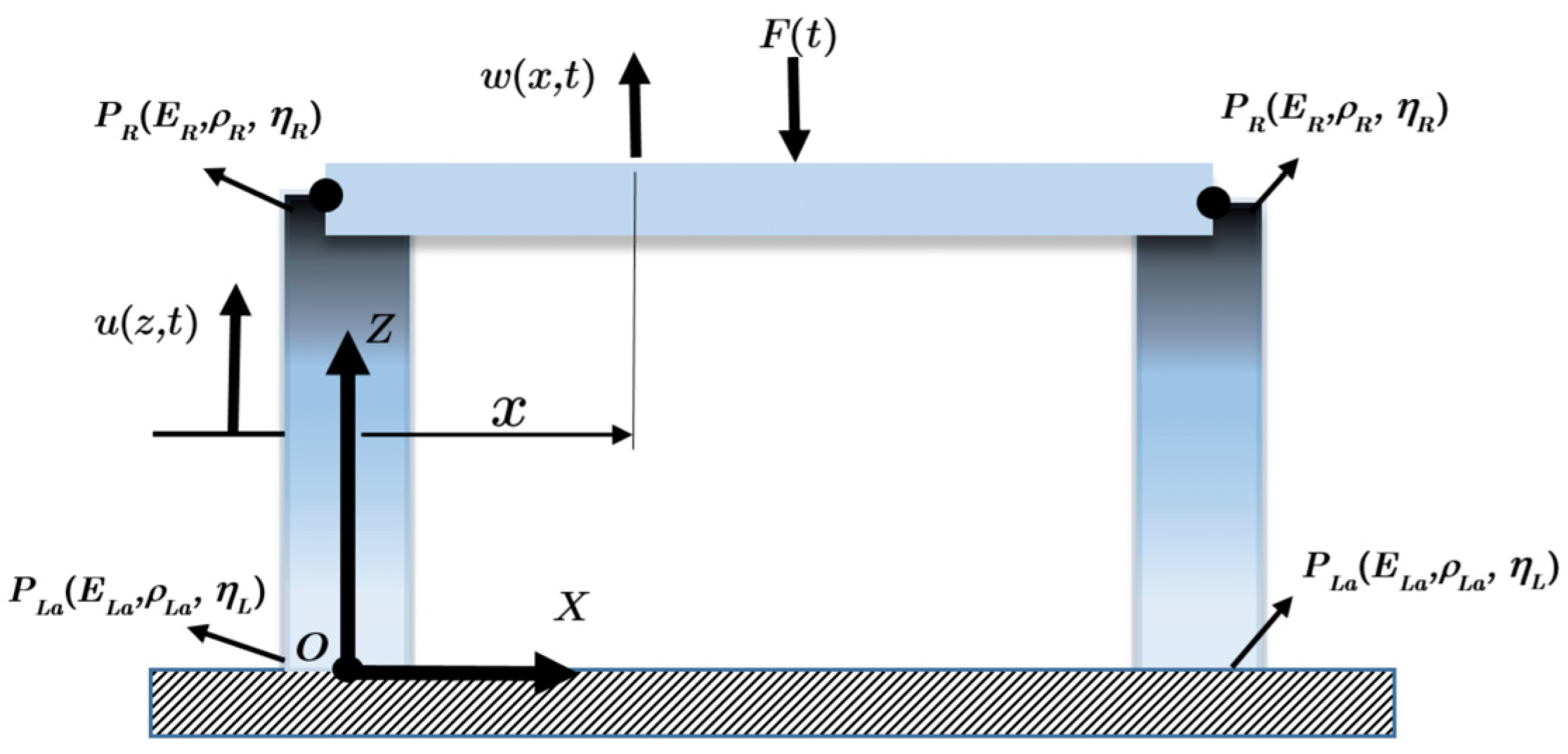
The system consists of beam and AFG viscoelastic bars. The system or only AFG viscoelastic bars can be used as an alternative to the spring and damping system to minimise the force transmitted to the ground in the foundations of large mass machines and to minimise the vibration amplitudes of machines. Variable internal damping and stiffness values along the axis of the structure at the support provide advantages in terms of stress and amplitude compared to other structures;

-

Passive dampers are used in buildings against stimuli such as earthquakes, wind, etc. Such energy dissipation devices are called ADAS (Added Damping and Stiffness). The ADAS can dissipate a part of the seismic energy input to a structure by hysteretic contribution. The structure considered in the paper absorbs large displacements, especially between floors, by axially varying internal damping. It is also safe in terms of structural stress;

-

In anti-terrorist structures such as mushroom barriers, it will be possible to make more successful anti-terrorist equipment by using the advantage of the varying stiffness and material damping of the rods in the axial direction (collision direction) in the steel pipe.

No study has been found in the literature on the vibration of viscoelastic FG bar-supported beams subjected to a harmonic force at the centre point. The evaluation of the effect of material dependent damping can be performed within the scope of harmonic analysis. The bars are connected to the end points of a beam by rotary joints to ensure that they work only in the axial direction. The damping effects of the materials, which are different on two surfaces in the axial direction, are defined as the product of Young’s modulus and the material damping coefficient and are assumed to vary along the bar depending on the exponential coefficient. A formulation is developed for the damping variation along the bar depending on the material. The values show exponential change with the material along the bar. The values of material damping are taken from the literature for axial displacement. Harmonic analyses are performed according to whether the ratio of the internal damping values between the two materials is greater or less than one. Eight material pairs are created. The effects of the length-varying material properties and internal damping of the FG support bars on the force transmission T_R and frequency parameters λ are examined in detail. The results are detailed in tables and graphs.

2. Theory and Formulations

An isotropic homogenous beam supported with viscoelastic axially FG bars is considered as shown in Figure 1. The beam is subjected to a sinusoidal force F(t) at the midpoint. It is assumed that the material properties of the bar vary longitudinally according to the power law distribution. The analysis of the harmonic forced vibration of a beam with the viscoelastic FG bar supports is proposed based on the equivalent complex stiffness coefficients. The beam has a length of L, thickness of h and width of b. The bar has a length of L_br, thickness of h_br and width of b_br. The beam is connected to the bars with pin joints to acquire pure axial deformation in the bars. Each structural element has a rectangular section. The Euler–Bernoulli beam theory governs the dynamic behaviour of the beam, with small deflections occurring in the x-z plane. The origin is chosen at the left end of the beam as shown in Figure 1. The dynamic behaviour of the bar is governed by the bar theory. The deflections of the bars and beam in the z and x direction are defined with u(z,t) and w(x,t), respectively. The bars are connected to the end points of a beam by rotary joints to ensure that they work only in the axial direction. The other ends of the bars are clamped. Kinetic energy and strain energy expressions are generated for the axial FG viscoelastic bar and beam. Element matrices obtained using Lagrange equations are assembled for the system. The force value and frequency parameters of the global system transmitted to the ground under harmonic force are analysed according to the material change coefficient of the axial element.

The material properties of bars at the two ends are define as follows. $E_{La}$: Young module of left surface material, $E_R$: Young module of right surface material, ${\rho }_{La}$: density of left surface material, ${\rho }_R$: density of right surface material, ${\eta }_L$: material loss factor of left surface material, ${\eta }_R$: material loss factor of right surface material, $P_{La}$: Young module of left surface material and $P_R$: Young module of right surface material.

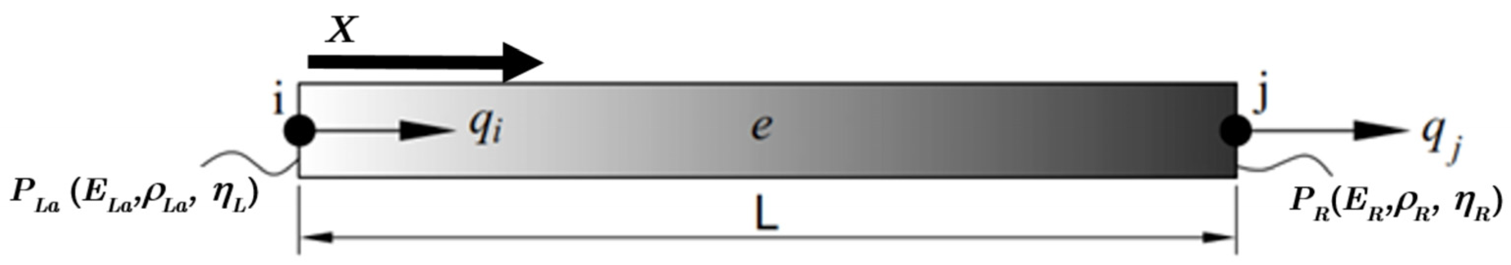
2.1. Finite Element Modelling of the Axial FG Element with Material Damping

Figure 2 shows a two-node finite element bar model “e”, which has a total length of L. The axial displacement is assumed in x direction along the bar, following the notation used in the literature for axial bar. The power law distribution determines the longitudinal variation of the material properties E(x), ρ(x) of the functionally graded bar. The function is defined as in Equation (1).

$$P(x)=(P_{La}-P_R){\left(1-{\displaystyle \frac{x}{L}}\right)}^{na}+P_R$$

(1)

where na is the power law exponent along the bar for material change.

The axial displacement of any point of the bar in the x direction is

$$u(x,z,t)=u_0(x,t)$$

(2)

Considering the strain and stress relationships of the axial bar within the framework of Hooke’s law, the elastic strain energy of a finite element at any time is

$$U={\displaystyle \frac{1}{2}}\underset{0}{\overset{L}{{\displaystyle \int }}}\underset{A}{{\displaystyle \int }}E\left(x\right){{\epsilon }_{xx}}^{2}dAdx$$

(3)

where ε_xx is the strain in x direction and for the area of the constant cross-section;

$$A={\displaystyle {\int }_{A}dA}$$

(4)

The variation of Young’s modulus can be expressed as follows, obeying Equation (1):

$$E\left(x\right)=\left(E_L-E_R\right){\left(1-{\displaystyle \frac{x}{L}}\right)}^{na}+E_R$$

(5)

At any given moment, the axial displacement resulting in the kinetic energy of the Axially Functionally Graded bar in Cartesian coordinates is

$$T={\displaystyle \frac{1}{2}}\underset{0}{\overset{L}{{\displaystyle \int }}}\underset{A}{{\displaystyle \int }}\rho (x){\dot{u}}^{2}dAdx$$

(6)

where $\dot{u}={\displaystyle \frac{du}{dt}}$ is the velocity of the axial element.

The variation of specific mass can be written as follows according to Equation (1):

$$\rho \left(x\right)=\left({\rho }_L-{\rho }_R\right){\left(1-{\displaystyle \frac{x}{L}}\right)}^{na}+{\rho }_R$$

(7)

Each node has one degree of freedom for the bar element. To express the axial displacement $u(x,t)$ of the element, the shape function and nodal displacements are used in matrix notation, as in Equation (8).

$$\left\{u\right\}={\left[N\right]}_{bx}\left\{\begin{array}{c}{q}_i\\ q_j\end{array}\right\}$$

(8)

The following extrapolation functions (Equation (9)) are used for the axial displacement along the bar:

$${\left[N\right]}_{bx}=\left\{1-{\displaystyle \frac{x}{L}} {\displaystyle \frac{x}{L}}\right\}$$

(9)

By substituting Equation (8) into Equations (3) and (6), the energy functions can be rewritten as follows:

$$U={\displaystyle \frac{1}{2}}\left({\left\{q\right\}}^T\left[A_{bx}A{\left[N^{\prime }\right]}_{bx}^T{\left[N^{\prime }\right]}_{bx}\right]\left\{q\right\}\right)$$

(10)

$$T={\displaystyle \frac{1}{2}}\left({\left\{\dot{q}\right\}}^T\left[\underset{0}{\overset{L}{{\displaystyle \int }}}\rho \left(x\right){\left[N\right]}_{bx}^T{\left[N\right]}_{bx}dx\right]\left\{\dot{q}\right\}\right)$$

(11)

where

$${\left[N^{\prime }\right]}_{bx}={\displaystyle \frac{d{\left[N\right]}_{bx}}{dx}}$$

(12)

$$A_{bx}=\underset{0}{\overset{L}{{\displaystyle \int }}}E\left(x\right)dx={\displaystyle \frac{\left(E_L-E_R\right)L}{na+1}}+E_{R}L$$

(13)

Using the expressions between the displacement and velocity terms from Equations (10) and (11), the stiffness and mass matrix can be written as in Equation (14).

$$\begin{array}{l} \left[K_A\right]=\left[A_{bx} A{\left[N^{\prime }\right]}_{bx}^T{\left[N^{\prime }\right]}_{bx}\right]\\ \left[M_A\right]=\left[\underset{0}{\overset{L}{{\displaystyle \int }}}\rho \left(x\right){\left[N\right]}_{bx}^T{\left[N\right]}_{bx}dx\right]\end{array}$$

(14)

Hysteretic damping is a better choice for proportional damping if it is proportional to the stiffness matrix, rather than viscous damping, and it is only proportional to the stiffness matrix. However, hysteretic damping can also be proportional to the mass matrix. When the excitation is harmonic, the structural form of damping can only be obtained by replacing Young’s modulus E with a complex one E(1 + iη). η is the material loss factor for isotropic homogenous bar. While deriving the element stiffness matrices, the complex matrix for material damping can be obtained as in Equation (15) [1,9].

$$\begin{gathered} \left[K\right]+i\left[H\right] \\ \left[H\right]=\eta \left[K\right] \end{gathered}$$

(15)

The axial damping coefficient is assumed to be proportional to Young modules by the loss factor. The Young’s modulus and loss factor are different at both ends and vary along the axis of the bar with the power exponential coefficient “na”. The internal viscous damping coefficient (Equation (16)), which is the product of these variables, will be used to define the axial hysteretic damping for ease of mathematical expression. It will be assumed that only this variable varies along the bar expressed in Equation (18).

$$c_A(x)=E(x)\eta (x)$$

(16)

where c_A is the internal damping coefficient and η is the longitudinal loss factor of the bar.

Considering that Young’s modulus and material damping change at the same rate and are material-specific, it is assumed that the Eη product changes depending on x in order to make the change linear, and the variation of Eη can be written as follows, according to Equation (17):

$$\begin{array}{c}{c}_{AL}=E_L{\eta }_L\\ c_{AR}=E_R{\eta }_R\\ c_A\left(x\right)=\left(c_{AL}-c_{AR}\right){\left(1-{\displaystyle \frac{x}{L}}\right)}^{na}+c_{AR}\end{array}$$

(17)

Complex stiffness matrix can be obtained as follows:

$$\begin{array}{c}\left[H\right]=\left(\underset{0}{\overset{L}{{\displaystyle \int }}}{c}_A\left(x\right)dx\right)\left[K\right]\\ \left[H\right]=\left[C_x {A{\left[N^{\prime }\right]}_{ax}}^T{\left[N^{\prime }\right]}_{ax}\right]\\ C_x=\underset{0}{\overset{L}{{\displaystyle \int }}}{c}_A\left(x\right)dx={\displaystyle \frac{\left(c_{AL}-c_{AR}\right)L}{na+1}}+c_{AR}L\end{array}$$

(18)

The expansions of the local mass, stiffness and complex stiffness matrices for the axial element in Equations (14) and (18) are as follows:

$$\begin{array}{l}{\left[M_A\right]}^e=\left[\begin{array}{cc}A.I_{Aa}-{\displaystyle \frac{2A.I_{Ba}}{L}}+{\displaystyle \frac{A.I_{Da}}{L^2}}& {\displaystyle \frac{A.I_{Ba}}{L}}-{\displaystyle \frac{A.I_{Da}}{L^2}}\\ {\displaystyle \frac{A.I_{Ba}}{L}}-{\displaystyle \frac{A.I_{Da}}{L^2}}& {\displaystyle \frac{A.I_{Da}}{L^2}}\end{array}\right]\\ {\left[K_A\right]}^e=\left[\begin{array}{cc}{\displaystyle \frac{A.A_{bx}}{L^2}}& -{\displaystyle \frac{A.A_{bx}}{L^2}}\\ -{\displaystyle \frac{A.A_{bx}}{L^2}}& {\displaystyle \frac{A.A_{bx}}{L^2}}\end{array}\right]\\ {\left[H\right]}^e=\left[\begin{array}{cc}{\displaystyle \frac{A.C_X}{L^2}}& -{\displaystyle \frac{A.C_X}{L^2}}\\ -{\displaystyle \frac{A.C_X}{L^2}}& {\displaystyle \frac{A.C_X}{L^2}}\end{array}\right]\end{array}$$

(19)

where

$$\begin{array}{l}{I}_{Aa}=\underset{0}{\overset{L}{{\displaystyle \int }}}\rho \left(x\right)dx={\displaystyle \frac{\left({\rho }_{La}-{\rho }_R\right)L}{n+1}}+{\rho }_{R}L\\ I_{Ba}=\underset{0}{\overset{L}{{\displaystyle \int }}}\rho \left(x\right)xdx={\displaystyle \frac{\left({\rho }_{La}-{\rho }_R\right)L^2}{\left(n+1\right)\left(n+2\right)}}+{\rho }_R{\displaystyle \frac{L^2}{2}}\\ I_{Da}=\underset{0}{\overset{L}{{\displaystyle \int }}}\rho \left(x\right)x^{2}dx={\displaystyle \frac{\left({\rho }_{La}-{\rho }_R\right)2L^3}{\left(n+1\right)\left(n+2\right)\left(n+3\right)}}+{\rho }_R{\displaystyle \frac{L^3}{6}}\end{array}$$

(20)

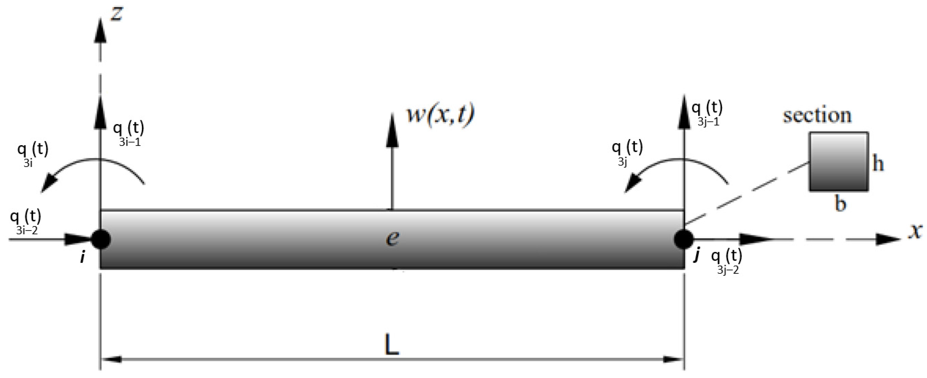
2.2. Modelling Beam Element

The degrees of freedom for a two-node finite element beam model with a total length of L are shown in Figure 3. It is assumed that the elastic modulus E, density ρ and Poisson’s ratio ν of the beam are constant.

In relation to Euler–Bernoulli beam theory, any point can have an axial and transverse displacement, as written in Equations (21) and (22), respectively.

$$u(x,z,t)=u_0(x,t)-z{\displaystyle \frac{\partial w_0(x,t)}{\partial x}}$$

(21)

$$w(x,z,t)=w_0(x,t)$$

(22)

Hooke’s law allows you to write the elastic strain energy of an element in Cartesian coordinates in the Euler–Bernoulli beam frame as in Equations (23) and (24):

$$U={\displaystyle \frac{1}{2}}{\displaystyle {\int }_V{\left\{\epsilon \right\}}^T\left\{\sigma \right\}dV}$$

(23)

$$U={\displaystyle \frac{1}{2}}{\displaystyle {\int }_0^L\left[A_{xx}{\left(\frac{\partial u_0}{\partial x}\right)}^2-2B_{xx}\left(\frac{\partial u_0}{\partial x}\right)\left(\frac{{\partial }^2{w}_0}{\partial x^2}\right)+D_{xx}\left(\frac{{\partial }^2{w}_0}{\partial x^2}\right)\right]}dx$$

(24)

where ε is strain components and σ is stress components. The other components of Equation (24) are written as in Equation (25a)–(25d).

$$A_{xx}={\displaystyle {\int }_{A}EdA}=Ebh$$

(25a)

$$B_{xx}={\displaystyle {\int }_{A}E\cdot zdA}=0$$

(25b)

$$D_{xx}={\displaystyle {\int }_{A}E\cdot z^{2}dA}={\displaystyle \frac{Eb{h}^3}{12}}$$

(25c)

$$A={\displaystyle {\int }_{A}dA}=bh$$

(25d)

Equation (26) gives the beam’s kinetic energy in Cartesian coordinates as a function of its bending at any time.

$$T={\displaystyle \frac{1}{2}}{\displaystyle {\int }_V\mathsf{\rho }\cdot ({\dot{u}}^2+{\dot{w}}^2})dV$$

(26)

$\dot{u}$ and $\dot{w}$ are the axial and transverse velocities, respectively. Extending Equation (26) and reducing the volume integral to a one-dimensional integral can result in Equation (27) being written.

$$T={\displaystyle \frac{1}{2}}{\displaystyle {\int }_0^L\left[I_A{\left(\frac{\partial u_0}{\partial t}\right)}^2-2I_B\left(\frac{\partial u_0}{\partial t}\right)\left(\frac{{\partial }^2{w}_0}{\partial x\partial t}\right)+I_A{\left(\frac{\partial w_0}{\partial t}\right)}^2+I_D{\left(\frac{{\partial }^2{w}_0}{\partial x\partial t}\right)}^2\right]}dx$$

(27)

where

$$I_A={\displaystyle {\int }_A\mathsf{\rho }dA}=\rho bh$$

(28a)

$$I_B={\displaystyle {\int }_A\mathsf{\rho }\cdot zdA}=0$$

(28b)

$$I_D={\displaystyle {\int }_A\mathsf{\rho }\cdot z^{2}dA}={\displaystyle \frac{\rho b{h}^3}{12}}$$

(28c)

As shown in Figure 3, every node has three degrees of freedom and all nodal degrees of freedom are given in Equation (29).

$$\left\{q\right\}={\left[q_{3i-2}\left(t\right),q_{3i-1}\left(t\right),q_{3i}\left(t\right),q_{3j-2}\left(t\right),q_{3j-1}\left(t\right),q_{3j}\left(t\right)\right]}^T$$

(29)

To express the transverse displacement (w(x,t)) and axial displacement (u(x,t)) with the nodal displacements, shape functions are used in matrix notation.

$$\left\{u\right\}={\left[N\right]}_{bx}\cdot {\left\{\begin{array}{c}{q}_{3i-2}\\ q_{3j-2}\end{array}\right\}}_u$$

(30)

$$\left\{w\right\}={\left[N\right]}_w\cdot {\left\{\begin{array}{c}{q}_{3i-1}\\ q_{3i}\\ q_{3j-1}\\ q_{3j}\end{array}\right\}}_w$$

(31)

Axial displacement and bending have their shape functions defined by [N]_bx and [N]_w, respectively.

By combining Equations (30) and (31) with Equations (24) and (27), the energy functions can be rewritten as follows:

$$U={\displaystyle \frac{1}{2}}{\displaystyle {\int }_0^L\left[A_{xx}{\left({\left[N^{\prime }\right]}_{bx}\cdot {\left\{q\right\}}_u\right)}^2+D_{xx}{\left({\left[N^{″}\right]}_w\cdot {\left\{q\right\}}_w\right)}^2\right]}dx$$

(32)

$$T={\displaystyle \frac{1}{2}}{\displaystyle {\int }_0^L\left[I_A{\left({\left[N\right]}_{bx}\cdot {\left\{\dot{q}\right\}}_u\right)}^2+I_A{\left({\left[N\right]}_w\cdot {\left\{\dot{q}\right\}}_w\right)}^2+I_D{\left({\left[N^{\prime }\right]}_w\cdot {\left\{\dot{q}\right\}}_w\right)}^2\right]}dx$$

(33)

Equations (32) and (33) are expanded as

$$U={\displaystyle \frac{1}{2}}\left[{{\left\{q\right\}}_u}^T\left(A_{xx}{\displaystyle {\int }_0^L{{\left[N^{\prime }\right]}_{bx}}^T{\left[N^{\prime }\right]}_{bx}dx}\right){\left\{q\right\}}_u+{{\left\{q\right\}}_w}^T\left(D_{xx}{\displaystyle {\int }_0^L{{\left[N^{″}\right]}_w}^T{\left[N^{″}\right]}_{w}dx}\right){\left\{q\right\}}_w\right]$$

(34)

$$T={\displaystyle \frac{1}{2}}\left[\begin{array}{l}{{\left\{\dot{q}\right\}}_u}^T\left(I_A{\displaystyle {\int }_0^L{{\left[N\right]}_{bx}}^T{\left[N\right]}_{bx}dx}\right){\left\{\dot{q}\right\}}_u+{{\left\{\dot{q}\right\}}_w}^T\left(I_A{\displaystyle {\int }_0^L{{\left[N\right]}_w}^T{\left[N\right]}_{w}dx}\right){\left\{\dot{q}\right\}}_w+\\ {{\left\{\dot{q}\right\}}_w}^T\left(I_D{\displaystyle {\int }_0^L{{\left[N^{\prime }\right]}_w}^T{\left[N^{\prime }\right]}_{w}dx}\right){\left\{\dot{q}\right\}}_w\end{array}\right]$$

(35)

The terms between the displacement and velocity vectors in Equations (34) and (35) give the stiffness and mass matrix as in Equations (36a) and (36b).

$$\left[K\right]=\left[\begin{array}{cccccc}{\displaystyle \frac{A_{xx}}{L}}& 0& 0& -{\displaystyle \frac{A_{xx}}{L}}& 0& 0\\ 0& {\displaystyle \frac{12D_{xx}}{L^3}}& {\displaystyle \frac{6D_{xx}}{L^2}}& 0& -{\displaystyle \frac{12D_{xx}}{L^3}}& {\displaystyle \frac{6D_{xx}}{L^2}}\\ 0& {\displaystyle \frac{6D_{xx}}{L^2}}& {\displaystyle \frac{4D_{xx}}{L}}& 0& -{\displaystyle \frac{6D_{xx}}{L^2}}& {\displaystyle \frac{2D_{xx}}{L}}\\ -{\displaystyle \frac{A_{xx}}{L}}& 0& 0& {\displaystyle \frac{A_{xx}}{L}}& 0& 0\\ 0& -{\displaystyle \frac{12D_{xx}}{L^3}}& -{\displaystyle \frac{6D_{xx}}{L^2}}& 0& {\displaystyle \frac{12D_{xx}}{L^3}}& -{\displaystyle \frac{6D_{xx}}{L^2}}\\ 0& {\displaystyle \frac{6D_{xx}}{L^2}}& {\displaystyle \frac{2D_{xx}}{L}}& 0& -{\displaystyle \frac{6D_{xx}}{L^2}}& {\displaystyle \frac{4D_{xx}}{L}}\end{array}\right]$$

(36a)

$$\left[M\right]=\left[\begin{array}{cccccc}{\displaystyle \frac{I_{A}L}{3}}& 0& 0& {\displaystyle \frac{I_{A}L}{6}}& 0& 0\\ 0& {\displaystyle \frac{13I_{A}L}{35}}+{\displaystyle \frac{6I_D}{5L}}& {\displaystyle \frac{11I_A{L}^2}{210}}+{\displaystyle \frac{I_D}{10}}& 0& {\displaystyle \frac{9I_{A}L}{70}}-{\displaystyle \frac{6I_D}{5L}}& -{\displaystyle \frac{13I_A{L}^2}{420}}+{\displaystyle \frac{I_D}{10}}\\ 0& {\displaystyle \frac{11I_A{L}^2}{210}}+{\displaystyle \frac{I_D}{10}}& {\displaystyle \frac{11I_A{L}^3}{105}}+{\displaystyle \frac{2I_{D}L}{15}}& 0& {\displaystyle \frac{13I_A{L}^2}{420}}-{\displaystyle \frac{I_D}{10}}& -{\displaystyle \frac{I_A{L}^2}{140}}+{\displaystyle \frac{I_{D}L}{30}}\\ {\displaystyle \frac{I_{A}L}{6}}& 0& 0& {\displaystyle \frac{I_{A}L}{3}}& 0& 0\\ 0& {\displaystyle \frac{9I_{A}L}{70}}-{\displaystyle \frac{6I_D}{5L}}& {\displaystyle \frac{13I_A{L}^2}{420}}-{\displaystyle \frac{I_D}{10}}& 0& {\displaystyle \frac{13I_{A}L}{35}}+{\displaystyle \frac{6I_D}{5L}}& -{\displaystyle \frac{11I_A{L}^2}{210}}-{\displaystyle \frac{I_D}{10}}\\ 0& -{\displaystyle \frac{13I_A{L}^2}{420}}+{\displaystyle \frac{I_D}{10}}& -{\displaystyle \frac{I_A{L}^2}{140}}+{\displaystyle \frac{I_{D}L}{30}}& 0& -{\displaystyle \frac{11I_A{L}^2}{210}}-{\displaystyle \frac{I_D}{10}}& {\displaystyle \frac{I_A{L}^3}{105}}+{\displaystyle \frac{2I_{D}L}{15}}\end{array}\right]$$

(36b)

2.3. Assembling the Matrices of System

Each element of the AFG bar is capable of axial deformation and each element of the beam is capable of both axial and bending deformation. Figure 2 and Figure 3 show typical elements together with its local axes, x and z, which are inclined to the global axes X and Z. The local axis of AFG bar “x” lies along the z-axis of the beam and the global axis Z in the assemblage. The degrees of freedom at both the nodes of AFG bar and beam elements can therefore be transformed from local to global axes by means of the relation, as can be seen from Figure 4.

The material change is defined along the bar by using Equation (1), as in Figure 2 and Figure 3.

In the assembly process, the degrees of freedom of beam are pb = 3m + 3, m is the number of the finite elements and n = m + 1 is the number of the nodes. Considering the axial FG bar elements as support with the beam, total degrees of freedom of the system can be written as in Equation (37).

$$p=3m+3+2ma$$

(37)

where last term “ma” belongs to the number of the elements of the axial FG bar and the degrees of freedom of axial FG bars are 2ma + 2. The number of elements of beam and each of axial FG bar is considered equal (64 elements).

The assembly process of the elements of matrices can be derived in Equation (38) as follows:

K(i, j) = K_A(i, j); i = 1…m, j = 1…m
K(m + i, m + j) = K_B(i, j), i = 1…pb, j = 1…pb
K(p + 1 − i, p + 1 − j) = K_A(i, j), i = 1…m, j = 1…m

(38)

The assembly process of the intersection elements of matrices can be derived for the left and right supports, respectively, as in Equation (39), as follows:

K(m, m + 2) = K_A(m, m + 1);
K(m + 2, m) = K_A(m + 1, m);
K(m + 2, m + 2) = K_A(m + 1, m + 1) + K(m + 2, m + 2);
K(4m + 2, 4m + 4) = K_A(p, p−1);
K(4m + 4, 4m + 2) = K_A(p−1, p);
K(4m + 2, 4m + 2) = K_A(p, p) + K(4m + 2, 4m + 2);

(39)

where K is the global stiffness matrix, K_A is the axial FG bar stiffness matrix and K_B is the beam stiffness matrix. The same assembly processes is applied to mass and complex stiffness matrices of the system elements.

After assembling the stiffness, complex stiffness and mass matrices, the global equations for a finite element model of the structure can be written by using the Lagrange equations. The set of differential equations governing the motion of the system is obtained considering the discrete (Equation (40)) and combined (Equation (41)) form of the system matrices as follows:

$$\left[K_B\right]\left\{q_B\right\}+\left(\left[K_A\right]+i\left[H\right]\right)\left\{q_A\right\}+\left[M_A\right]\left\{{\ddot{q}}_A\right\}+\left[M_B\right]\left\{{\ddot{q}}_B\right\}=\left\{F(t)\right\}$$

(40)

$$\left[K\right]\left\{q\right\}+i\left[H\right]\left\{q\right\}+\left[M\right]\left\{\ddot{q}\right\}=\left\{F(t)\right\}$$

(41)

The harmonic force acting at the centre of the beam is expressed as follows in Equation (42)

$$\left\{F(t)\right\}=\left\{F_{\max }\right\}·e^{i\omega t}$$

(42)

$\left\{F(t)\right\}$ is $p\times 1$, a non-dimensional load vector. F_max is the magnitude of force acting on the midpoint of the beam and is the only non-zero term in the force vector on the ((p − 1)/2) + 1 row. Time-dependent nodal displacements for steady-state vibrations of the system can be written as follows:

$$\left\{q(t)\right\}=\left\{q_o\right\}{e}^{i\omega t}$$

(43)

The elements of $\left\{q_o\right\}$ are complex variables containing a phase angle. Substituting Equation (43) into Equation (41), the differential equation governing the motion can be written in the following form as in Equation (44), with the applied clamped boundary conditions for q₁ and q_p being zero. Subscript “s” in Equation (44) stands for the matrices with the boundary condition applied.

$$\left(\left[K_s\right]+i\left[H_s\right]-{\omega }^2\left[M_s\right]\right)\left\{q_o\right\}=\left\{F_{\max }\right\}$$

(44)

At nodes 1 and p, since the system is clamped (Figure 4), reaction forces $R_1$ and $R_p$ occur. In the global stiffness matrix, only K(1, 2) and K(p, p − 1) elements remain non-zero after boundary conditions are applied. Multiplying these elements by the corresponding displacements (q(2, 1) and q(p, p − 1)) gives the total reaction forces (Equation (45)).

The maximum total magnitude of reaction forces (also defined as force transmitted to ground) at the clamped ends and its ratio by maximum force F_max can be defined as force transmissibility T_R (Equation (46)).

$$\begin{array}{l}{R}_1=\left(\left(K(1,2)+iH(1,2)\right)-{\omega }^{2}M(1,2)\right)q_2\\ R_p=\left(\left(K(p,p-1)+iH(p,p-1)\right)-{\omega }^{2}M(p,p-1)\right)q_{\left(p-1\right)}\end{array}$$

(45)

$$T_R=\left[{\displaystyle \frac{R_1+R_p}{F_{max}}}\right]$$

(46)

3. Numerical Formulations

The dimensionless frequency parameters of the system are obtained numerically from the harmonic analysis. The system consists of the beam supported at the ends by the AFG bars. The code used for simulations is written according to the theory described above. The numerical investigations are performed in MATLAB on a workstation computer (2 × CPU of 3.3 GHz, 30 GB RAM). The numerical results are given in dimensionless form using Equation (47) for comparison with results in the literature.

$${\lambda }^2={\displaystyle \frac{{\rho }_{L}A{\omega }^2{L}^4}{E_{L}I}},F_B={\displaystyle \frac{F_{\max }{L}^2}{E_{L}I}}$$

(47)

where F_B is the non-dimensional form of force, λ is the non-dimensional frequency parameter and I is the moment of inertia of the area.

Equation (48) can be written in the following form using the relations of Equation (47):

$$\left(\left(\left[K_S\right]+i\left[H_S\right]\right)-{\lambda }^2\left[M_S\right]\right)\left\{q_o\right\}=\left\{F_B\right\}$$

(48)

The investigation is carried out by implementing different power law exponent (na) values and changing the materials at the ends of axial FG bars to investigate the effect of material distribution on the response frequency and the force transmissibility.

The left surface material of the bar (E_La, ρ_La, c_La) and the right surface material of the bar (E_R, ρ_R, c_R) are selected from the materials in

Table 1. Material properties [8].

	E (GPa)	ρ (kg/m3)	Flexural Loss Factor $\mathit{\eta }$	Longitudinal Loss Factor * $\mathit{\eta }$	${\mathit{c}}_{\mathit{A}}=\mathit{E}\mathit{\eta }$ (GPa)
Al/Aluminium	72	2700	(0.3–10) × 10−5	1 × 10−4	72 × 105
St/Steel	210	7800	(0.2–3) × 10−4	3 × 10−4	630 × 105
Br/Brass	95	8500	(0.2–1) × 10−3	1 × 10−3	950 × 105
Ag/Silver	80	10,500	4 × 10−4	3 × 10−3	2400 × 105
Cu/Copper (polycrystalline)	125	8900	2 × 10−3	2 × 10−3	2500 × 105
Pb/Lead(pure)	17	11,300	(5–30) × 10−2	2 × 10−2	3400 × 105

* The values are used in the study

. The material properties and damping values are taken from the literature [8]. The values in Table 1 are ranked from low to high, taking into account the longitudinal loss factor and c_A. The physical properties of the materials used in the numerical methods are taken from Table 1.

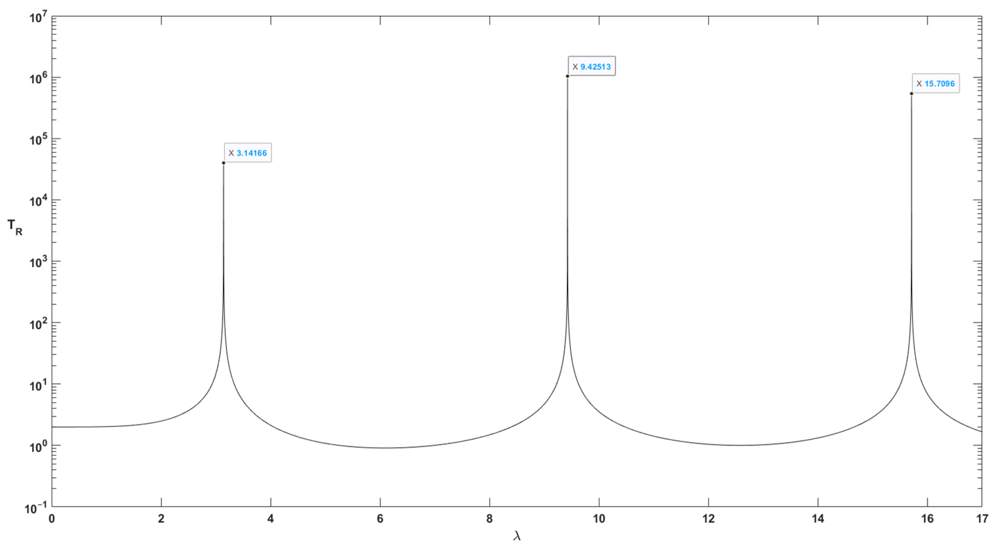
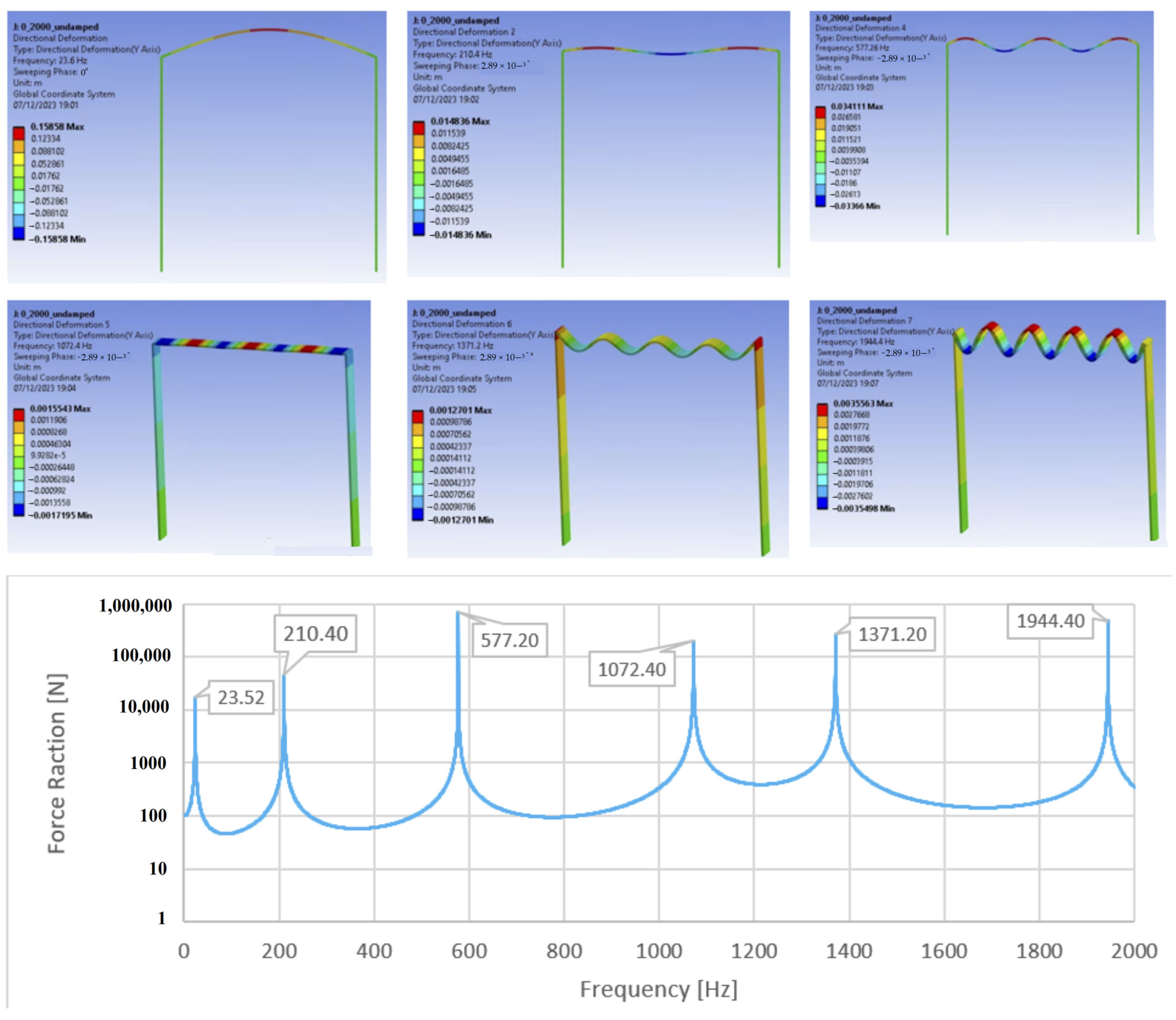
4. Verification Studies

No study has been found in the literature on the vibration of viscoelastic FG bar-supported beams subjected to a harmonic force at the centre point. Therefore, the frequency parameters of the simply supported beam [11] are used to verify the simulation results. The simply supported boundary condition is obtained by making the bar supports rigid. The value of Young’s modulus E of beam is 2.1 × 10¹¹ N/m² for the steel beam. Infinite axial stiffness can be simulated by setting the values of E_La and E_R equal to 70 × 10⁸⁰ N/m² and na = 1 for the axial bars. Figure 5 shows the force transmissibility of a steel beam supported with rigid bars, obtained in a MATLAB environment. The scanning interval is taken as 10⁻⁸ Hz when calculating the frequency parameters in all the tables for the harmonic analysis of the system in MATLAB. Considering the simulation time in graphical representations, the scanning interval for harmonic analysis in MATLAB is assumed to be 0.01 Hz. Consequently, the calculated results are compared with the exact results of the simply supported isotropic steel beam in

Table 2. Comparison of the results with the results of the literature.

Matlab Calculated Results			Rao’s Analytical Solution [11]	Ansys Workbench Modal Analysis		Ansys Workbench Harmonic Analysis
Non-Dimensional		Hz.	Non-Dimensional	Hz.	Non-Dimensional	Hz.	Non-Dimensional
SS1	3.14166	23.5293	3.1416	23.524	3.1413	23.52	3.14166
-	-	-	94.05	6.2798	-	-
SS2	9.42497	211.764	9.4248	211.44	9.4177	210.48	9.40425
	-	-	-	375.45	12.5389	-	-
SS3	15.7096	588.3315	15.708	585.76	15.6752	577.2	15.592

. The exact results are obtained using Rao’s analytical values [11].

The finite element model is also created with 3-D truss and beam elements in ANSYS to compare and visualise the results. To better understand the effect of the bar and beam on the vibration response, simulations are performed in the ANSYS environment. Three-dimensional truss and beam elements are connected with revolute joints. The system is fixed at the ends of aluminium bars. In addition, out-plane nodal rotation and displacements of the system are fixed to obtain in-plane motion (Figure 6). In the Ansys model, 64 elements are used for each of the beams and bars as in the Matlab model. The bars and beam have a rectangular cross-section with a width of 100 mm and a height of 10 mm. Their length is 1000 mm.

Harmonic analysis is performed between 0 and 2000 Hz. The frequency response and vibration motions obtained are shown in Figure 7. Table 2 compares the results of this study with the results of the Ansys harmonic and modal analysis under the same boundary conditions. Since there is a harmonic force acting on the centre point of the beam, antisymmetric modes are not seen. Symmetry–symmetry modes are visible in my study and Ansys harmonic analysis. The harmonic response of the steel beam supported by rigid bars is shown in Figure 7. All frequency parameters are only available in modal analysis. The results are quite close to each other. As shown in the displacement fringe of Figure 7, the displacement of the bars is higher in the forced vibration response at 1371.2 Hz. Therefore, the bar supports are more effective in the vibration motion. The hysteresis damping definition is predicted to be most effective for the bar-supported beam at this frequency. In addition, it will be more effective in reducing the force transmitted to the ground by acting as a support to the beam at the bar dominant frequency peaks when we consider the material damping.

5. Parameterisation Studies

Young’s modulus, area and length of the support bar affect its stiffness. The Young’s modulus change and its variation along the bar is controlled by the coefficient na. Taking the bar and beam length as a variable causes a change in the finite element length. This leads to convergence problems. Therefore, the lengths are assumed to be equal and 1 m.

Analyses are performed to see the effect of FG bar area and material damping on the force transmission. This part of study is carried out to reduce the combination of material pairs for the FG axial bar and to determine the area parameter in the most efficient way. The area and possible material pairs is determined for the lowest force transmission for the FG bar.

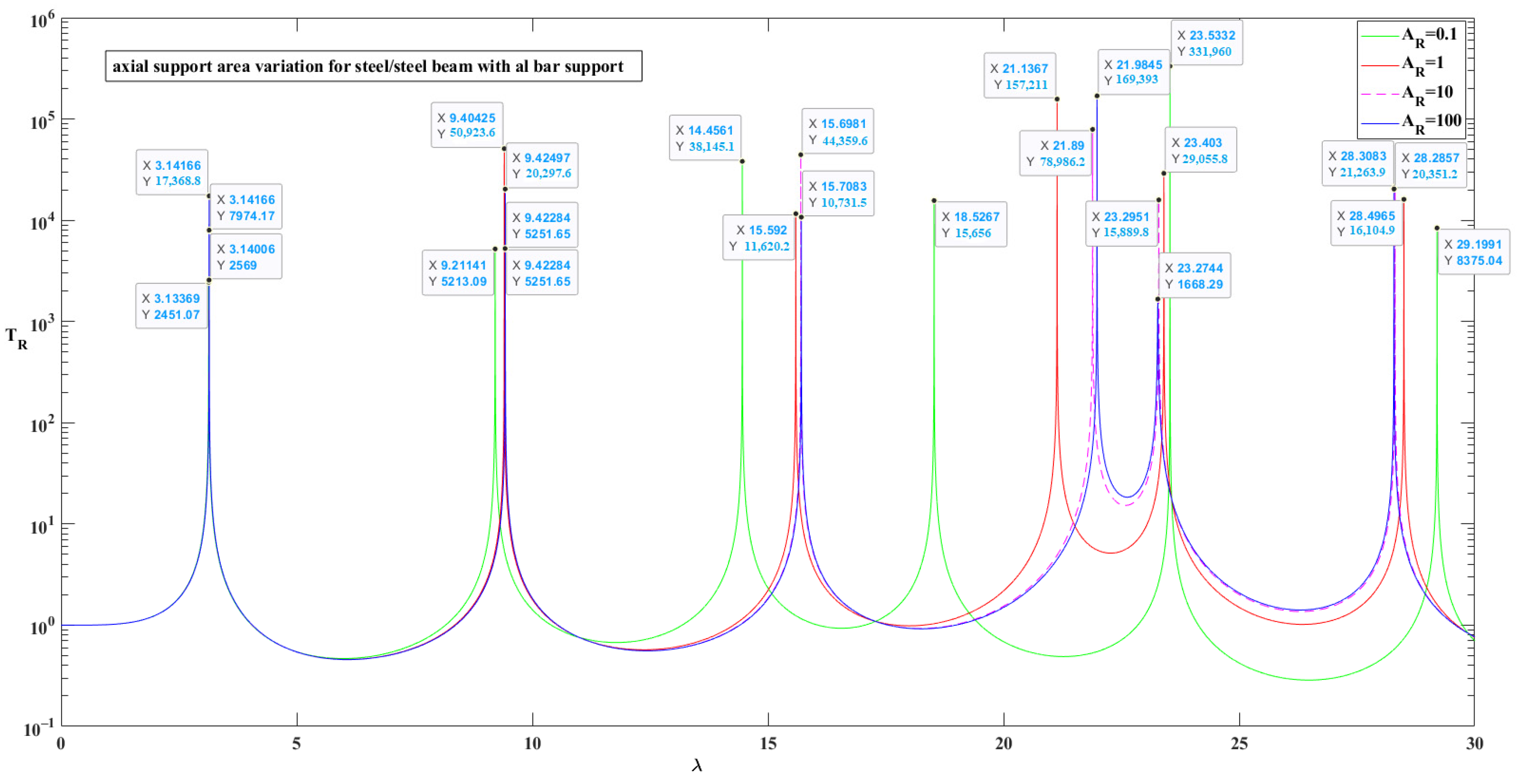
5.1. The Area of Support Bars

The stiffness parameter of the bar depends on the area so in order to see the effect of the area of the bar, the ratio of the area of the bar to the beam is introduced as A_R. To determine the A_R value for the support bar, only lead and aluminium materials are used in the calculations for brevity. Figure 8 and Figure 9 show the force transmission response of the lead bar supported and the aluminium bar supported beam in the frequency domain.

As can be seen from Figure 8 and Figure 9, frequency parameters generally increase with the increase in bar area. However, this situation is reversed after the bar effect is seen as a frequency parameter in the system. For example, in Figure 8, the frequency values increase with decreasing area in the peak responses around 15 and 22 Hz. In Figure 9, when the bar effect is seen in the frequency response, the frequency parameter increases with decreasing area around 23 and 28 Hz. At the frequencies where the response of the bar is dominant, the amplitudes of the frequency response decrease with increasing area around 11.31 Hz, 19.73 Hz and 25.45 Hz in Figure 8 and 23.27 Hz in Figure 9. The minimum transmission at these frequencies occurs when the value of A_R is 100. The minimum force transmission occurs at A_R variable 0.1 and 100 values for the aluminium bar-supported beam. This is due to the effective participation of the axial bar in the vibration, as mentioned above. If the beam is dominant in the vibration motion, the force transmission is minimal at 0.1 of A_R (3.13 Hz and 9.21 Hz) and if the bar is dominant, the force transmission is minimal at 100 of A_R (23.27Hz). One of these values (0.1 or 100) can make the force transmission minimum at one frequency peak and maximum at the other. Therefore, the area for the axial bar is chosen to be 10 times the area of the beam. In force transmission, the first frequency peak value is minimum for the lead and aluminium material used for the axial bar for A_R = 10.

5.2. Material Damping Effect

In order to see the effect of the material damping effect on the force transmission of the system, the material of the bar is taken as lead. It is seen that material damping is more effective in the peaks after the first frequency peak. It is also seen that if the material damping is zero, the force transmission increases excessively at each peak (actually expected to go on forever). In the case of damped axial bars, the force transmission decreases significantly. The effect of damping increases with increasing frequency. In the frequency responses of the system between 0 and 30 Hz, separating the peaks as SS1, SS2, SS3, SS4 and SS5 when the beam frequencies are dominant and as 1.Region, 2.Region, 3.Region and 4.Region when the bar frequencies are dominant provides a good approach to examining the damping effect and frequency changes. The results are tabulated in

Table 3. Force transmissibility values of the lead supported beam with material damping.

Pb Bar	SS1.Mod		SS2.Mod		1.Region		SS3.Mod		2.Region
	λ	TR	λ	TR	λ	TR	λ	TR	λ	TR
η = 0	3.141285	4,906,936	9.410127	11,465,955	11.33643	16,651,019	15.71125	62,202,302	19.62624	19,008,059
η = 0.2	3.141285	243,782	9.410127	6144	11.33643	61	15.71125	4056	19.627	18
	SS4.Mod		3.Region		SS5.Mod
	λ	TR	λ	TR	λ	TR
η = 0	22.00275	44,959,291	25.3654	101,320,433	28.27558	11,728,774
η = 0.2	22.00275	1412	25.3654	10	28.27558	619

and also given in Figure 10. This approach is used in all subsequent graphs.

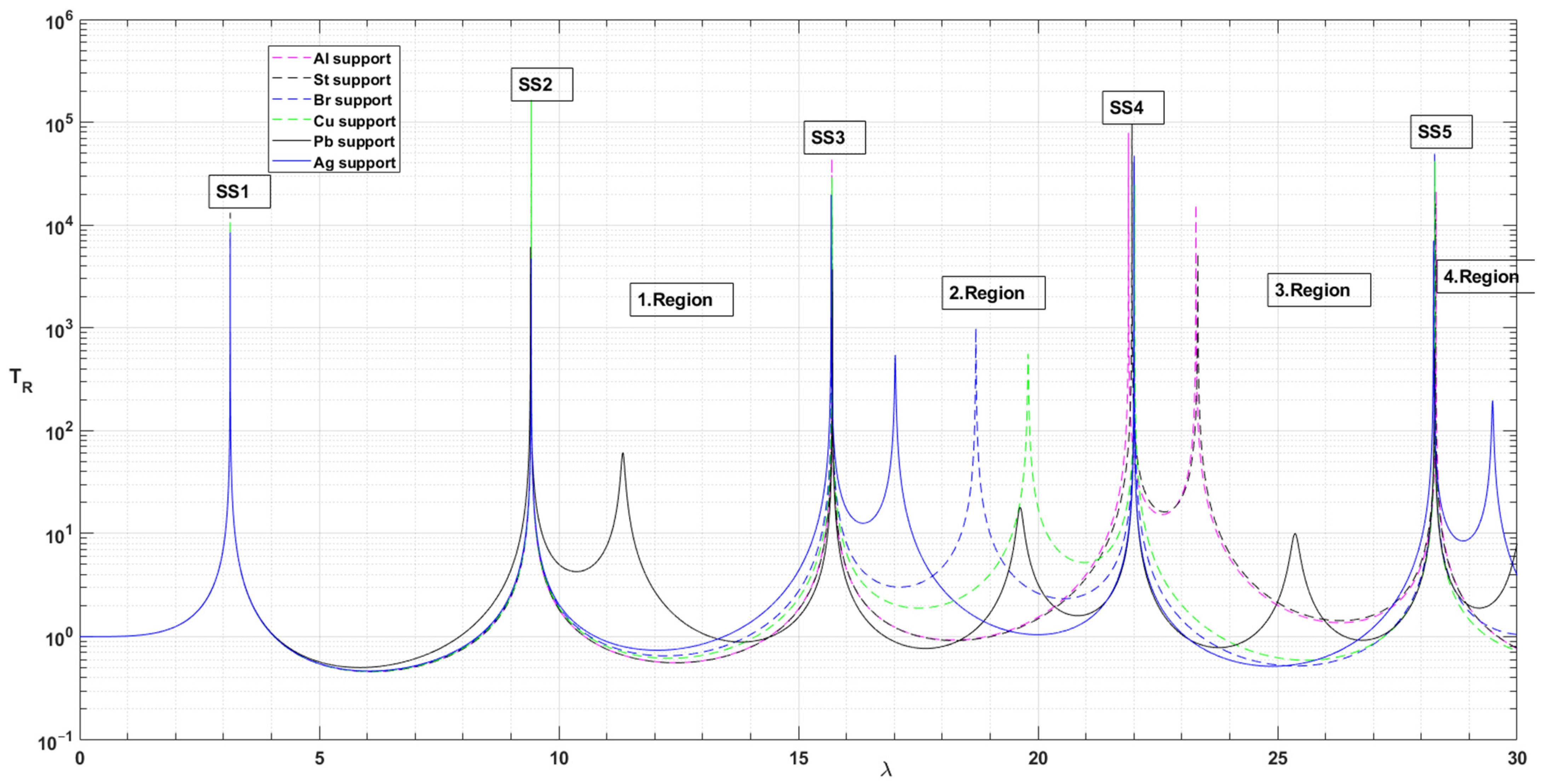
5.3. Material Pairs for Bar Support

The force transmission of a steel beam supported with the isotropic bars is investigated. The axial bar used to support the steel beam is formed isotropically from the materials St, Al, Br, Ag, Cu and Pb (Table 1). The maxima of the frequency and force transmission values are given in

Table 4. (a) Maximum frequency parameter and force transmission values of the system for bar supports consisting of various materials (c_A sequential). (b) Maximum frequency parameter and force transmission values of the system for bar supports consisting of various materials (Young’s module sequential).

(a)
Bar Material	Pb		Cu		Ag		Br		St		Al
Mode Number	λ	TR	λ	TR	λ	TR	λ	TR	λ	TR	λ	TR
SS1	3.14128	243,782	3.14156	14,412,284	3.14154	1,789,396	3.14155	2,004,509	3.14158	8,340,324	3.14153	8,287,499
SS2	9.41013	6144	9.42390	651,465	9.42313	271,842	9.42349	983,524	9.42441	3,849,090	9.42304	6,501,443
1.Region	11.33643	61
SS3	15.71125	4056	15.70121	108,121	15.68292	24,358	15.69666	143,805	15.70562	1,432,198	15.69806	1,460,498
2.Region	19.62722	18	19.79233	558	17.01995	544	18.70356	998
SS4	22.00275	1412	22.01536	45,711	22.00044	46,618	22.00860	115,014	21.95969	183,227	21.88989	186,157
3.Region	25.36540	10							23.33434	5348	23.29497	16,457
SS5	28.27558	619	28.28267	48,419	28.25448	7200	28.27770	61,126	28.29214	476,127	28.30824	499,885
4.Region					29.48704	195
(b)
Bar Material	St		Cu		Br		Ag		Al		Pb
Mode Number	λ	TR	λ	TR	λ	TR	λ	TR	λ	TR	λ	TR
SS1	3.14158	8,340,324	3.14156	14,412,284	3.14155	2,004,509	3.14154	178,9396	3.14153	8,287,499	3.14128	243,782
SS2	9.42441	3,849,090	9.42390	651,465	9.42349	983,524	9.42313	271,842	9.42304	6,501,443	9.41013	6144
1.Region											11.33643	61
SS3	15.70562	1,432,198	15.70121	108,121	15.69666	143,805	15.68292	24,358	15.69806	1,460,498	15.71125	4056
2.Region			19.79233	558	18.70356	998	17.01995	544			19.62722	18
SS4	21.95969	183,227	22.01536	45,711	22.00860	115,014	22.00044	46,618	21.88989	186,157	22.00275	1412
3.Region	23.33434	5348							23.29497	16,457	25.36540	10
SS5	28.29214	476,127	28.28267	48,419	28.27770	61126	28.25448	7200	28.30824	499,885	28.27558	619
4.Region							29.48704	195

and Figure 11. The effects of the materials on the force transmission are analysed for the isotropic case and an idea is gained for the material formation of FG pairs. To better understand the variations in frequency parameters and force transmission, the bar materials are ranked by Young’s modulus and internal damping coefficient (c_A) in Table 4.

Due to the harmonic force acting from the centre of the beam, only SS mode vibrations occur in the frequency response. The frequency response of the system can be considered to be two parts. Some frequency components belong to the beam’s dominant motion; the others belong to the bars’ dominant motion. With the addition of bars, side frequencies appear depending on the bars’ material. For the Pb material bar, after all SS modes, side frequency peaks are observed. The side frequency peaks appear at 3.Region for St and Al material; 2.Region for Cu and Br material, 2.Region; and 4.Region for Ag material. The location of the side peaks in the frequency response depends on the specific mass and Young’s modulus of the materials. Since Pb is the material with the lowest Young’s modulus and the highest specific mass, the first side peak appears in the frequency range at the lead bar (Figure 11).

Table 4a,b show the frequency values and maximum forces transmitted to the ground according to the internal damping coefficients (c_A) and Young’s modulus of the bar materials. The values of the force transmitted to the ground (T_R) decrease as the frequency parameter (λ) increases. The Pb, Ag and Br materials provide this for all modes. The Cu, St and Al materials give this for all modes except SS5 mode. The values of the force transmitted to the ground (T_R) decrease with the increase in the c_A value (Table 4a). All materials give this for all modes except Ag material. As can be seen from Table 4b, the values of λ decrease with the decrease in the E value for SS1, SS2 and SS5 modes of all materials. Although the other modes follow a trend, there is no general order. In the regions between the SS frequency peaks, the T_R values can be provided region by region with different materials below the value of 1 (Figure 11).

Depending on the material, the axial bar is effective on the frequency response. In addition to the frequencies where the beam is effective, frequencies where the axial bar is effective occur. The effect of the material change in the bar support is more dominant in Pb material (Figure 11).

When analysing the change in frequency as a function of the E of the bars in Table 4b, the changes in frequency are smaller in the SS modes, while the changes are larger in the modes dominated by bar motion. As can be seen from Table 4b, the changes in ca have a greater effect on Tr. The lowest values are obtained for the Pb material. In general, it is seen that the bar support with lead material is the most effective in terms of reducing force transmission at peaks (Figure 11).

5.4. The Limits of Material Distribution Coefficient “na”

A study is carried out to determine the limits of the material change coefficient na. Figure 12 shows that Young’s modulus changes depending on the material change coefficient for the different material pairs. When na goes from 0 to 10,000, the material changes from one to another obeying Equation (11). As there is almost no change in Young’s modulus after na = 100, numerical evaluations were made up to na = 100.

6. Investigation of Force Transmission of Axial FG Bar Supported Steel Beam According to Material Distribution Coefficient “na”

In this case, it is shown how bars made from combinations of different materials affect the level of force transmission by using na values. As can be seen from the previous section, lead is the most effective material for the bar considering force transmission. Therefore, material pairs are formed with the Pb and others. The material pairs for the bars are Al-Pb, Ag-Pb, Cu-Pb, Pb-Pb, Pb-Cu, Pb-Br, Pb-St and Pb-Al. The Young’s modulus, specific gravity, hysteresis and internal damping coefficient ratios of the material pairs are given in

Table 5. Material pairs and ratio values of material properties.

	E Ratio	ρRatio	ηRatio	CA (Eη) Ratio
Al/Pb	4.235294118	0.238938053	0.005	0.021176
Ag/Pb	4.705882	0.929204	0.15	0.705882
Cu/Pb	7.352941176	0.787610619	0.1	0.735294
Pb/Pb	1	1	1	1
Pb/Cu	0.136	1.269662921	10	1.36
Pb/Br	0.178947368	1.329411765	20	3.578947
Pb/St	0.080952381	1.448717949	66.66667	5.396825
Pb/Al	0.236111111	4.185185185	200	47.22222

. The ratio of Eη is ranked from the smallest to the largest value below and above one as can be seen in Table 5. Using the material ranking in Table 5, the frequency-dependent variation of the force transmission at different ratios of the material change coefficient na is analysed. The values of 0, 0.2, 0.5, 1, 2, 5, 10 and 100 are taken for na. The force transmission response of the system is plotted in the range of 0–30 Hz using a step interval of 0.01 Hz in Figure 13, Figure 14, Figure 15, Figure 16, Figure 17, Figure 18 and Figure 19. The step interval is set to 10⁻⁸ Hz to obtain more accurate results for

Table 6. Frequency parameters and force transmission coefficient variations for the material pairs c_Aratio < 1.

Al/Pb
	SS1		SS2		1.Region		SS3		2.Region		SS4		3.Region		SS5		4.Region
na	λ	TR	λ	TR	λ	TR	λ	TR	λ	TR	λ	TR	λ	TR	λ	TR	λ	TR
0	3.14153	4,584,299	9.42304	167,778			15.69806	32,607			21.89002	4121	23.29653	364	28.30827	11,053
0.2	3.14152	4,207,768	9.42270	152,565			15.69360	26,052	20.12809	288	22.04616	8639			28.28465	11,791
0.5	3.14150	3,862,223	9.42221	138,182			15.68285	17,694	18.01204	272	22.01073	20,042			28.26654	7038
1	3.14148	3,580,055	9.42148	125,492			15.61944	6135	16.3106	939	21.99940	22,155	27.95853	572	28.45400	1083
2	3.14145	3,462,921	9.42027	117,195	14.58257	635	15.75101	15,768			21.98918	16,872	25.34486	114	28.29201	9297
5	3.14140	4,079,769	9.41782	128,369	13.03908	556	15.72294	54,267			21.93939	6176	22.67103	543	28.24702	5210	29.25848	230
10	3.14136	6,035,680	9.41561	177,822	12.29681	962	15.71748	98,712	21.26622	887	22.04542	11,981	27.49573	495	28.32821	7589
100	3.14129	22,650,047	9.41101	584,055	11.44642	5305	15.71201	380,530	19.81652	1681	22.00516	126,262	25.61121	919	28.28022	60,951
Ag/Pb
	SS1		SS2		1.Region		SS3		2.Region		SS4		3.Region		SS5		4.Region
na	λ	TR	λ	TR	λ	TR	λ	TR	λ	TR	λ	TR	λ	TR	λ	TR	λ	TR
0	3.14154	13,158,012	9.42314	466,260			15.68292	41,757	17.0200	933	22.00044	79,919			28.25449	12,346	29.48763	335
0.2	3.14153	8,873,608	9.42280	311,797			15.65846	17,146	16.40639	1293	21.99842	54,963			28.12347	1839	28.51182	1289
0.5	3.14151	5,779,456	9.42233	200,653	15.48819	3065	15.87273	4152			21.99590	34,187	27.1014	203	28.31277	6937
1	3.14149	3,562,337	9.42162	121,426	14.8179	589	15.75018	12,243			21.99206	18,399	25.7453	89	28.29311	8803
2	3.14146	2,010,061	9.42043	66,390	13.9188	235	15.72914	16,487			21.98348	7521	24.1620	69	28.28054	5306
5	3.14141	973,785	9.41800	30,124	12.8090	124	15.71993	14,074			21.88856	756	22.31571	255	28.21306	673	28.76369	103
10	3.14137	643,107	9.41578	18,741	12.2010	100	15.71644	10,660	21.11088	76	22.03336	1575	27.291	41	28.31509	1020
100	3.14130	373,432	9.41106	9617	11.4399	87	15.71195	6270	19.80615	28	22.00495	2087	25.59731	15	28.27998	1002
Cu/Pb
	SS1		SS2		1.Region		SS3		2.Region		SS4		3.Region		SS5		4.Region
na	λ	TR	λ	TR	λ	TR	λ	TR	λ	TR	λ	TR	λ	TR	λ	TR	λ	TR
0	3.141562	28,114,214	9.42390	1,017,914			15.70121	168,945	19.79246	872	22.01536	81,417			28.28267	75,668
0.2	3.141555	18,833,545	9.42368	678,206			15.69838	101,115	18.83889	608	22.00813	75,307			28.27891	43,397
0.5	3.141545	12,000,457	9.42336	428,744			15.69245	52,117	17.81276	537	22.00351	65,012			28.27133	20,057
1	3.141529	7,077,611	9.42287	249,716			15.67188	18,040	16.68968	732	21.99957	43,784			28.22471	3846	28.92619	364
2	3.141503	3,674,291	9.42198	126,709	15.25034	1053	15.79087	5870			21.99452	20,816	26.55739	105	28.30251	6522
5	3.141450	1,499,524	9.41995	48,985	13.67858	175	15.72676	14,428			21.97888	4853	23.74623	64	28.27621	3604
10	3.141403	855,290	9.41777	26,337	12.75307	111	15.71968	12,581			21.85889	534	22.24804	291	28.19220	472	28.65825	118
100	3.141304	376,660	9.41166	9854	11.51472	84	15.71244	6362	19.93583	28	22.00662	2034	25.76523	15	28.28288	1034

,

Table 7. Frequency parameters and force transmission coefficient variations for the material pairs c_Aratio = 1.

Pb/Pb
	SS1		SS2		1.Region		SS3		2.Region		SS4		3.Region		SS5		4.Region
na	λ	TR	λ	TR	λ	TR	λ	TR	λ	TR	λ	TR	λ	TR	λ	TR	λ	TR
0	3.141285	243,782	9.410127	6144	11.33643	61	15.71125	4056	19.627	18	22.00275	1412	25.3654	10	28.27558	619
0.2	3.141285	243,782	9.410127	6144	11.33643	61	15.71125	4056	19.627	18	22.00275	1412	25.3654	10	28.27558	619
0.5	3.141285	243,782	9.410127	6144	11.33643	61	15.71125	4056	19.627	18	22.00275	1412	25.3654	10	28.27558	619
1	3.141285	243,782	9.410127	6144	11.33643	61	15.71125	4056	19.627	18	22.00275	1412	25.3654	10	28.27558	619
2	3.141285	243,782	9.410127	6144	11.33643	61	15.71125	4056	19.627	18	22.00275	1412	25.3654	10	28.27558	619
5	3.141285	243,782	9.410127	6144	11.33643	61	15.71125	4056	19.627	18	22.00275	1412	25.3654	10	28.27558	619
10	3.141285	243,782	9.410127	6144	11.33643	61	15.71125	4056	19.627	18	22.00275	1412	25.3654	10	28.27558	619
100	3.141285	243,782	9.410127	6144	11.33643	61	15.71125	4056	19.627	18	22.00275	1412	25.3654	10	28.27558	619

and

Table 8. Frequency parameters and force transmission coefficient variations for the material pairs c_Aratio > 1.

Pb/Cu
	SS1		SS2		1.Region		SS3		2.Region		SS4		3.Region		SS5		4.Region
na	λ	TR	λ	TR	λ	TR	λ	TR	λ	TR	λ	TR	λ	TR	λ	TR	λ	TR
0	3.14128	193,155	9.41013	4859	11.33616	48	15.71126	3207	19.62689	14	22.00274	1116	25.36241	8	28.27551	489
0.2	3.14145	849,163	9.41995	27,746	13.68093	99	15.72678	8160			21.97891	2752	23.74845	36	28.27619	2041
0.5	3.14150	2,020,898	9.42198	69,706	15.25409	584	15.79143	3205			21.99452	11,449	26.56335	58	28.30255	3576
1	3.14153	3,768,639	9.42287	132,984			15.67205	9650	16.69442	388	21.99957	23,295			28.22535	2069	28.93241	192
2	3.14154	6,162,435	9.42336	220,193			15.69248	26,814	17.81772	275	22.00352	33,341			28.27135	10,319
5	3.14156	9,284,181	9.42368	334,349			15.69839	49,885	18.84243	300	22.00814	37,076			28.27891	21,399
10	3.14156	10,969,268	9.42379	396,089			15.69988	62,487	19.28222	337	22.01092	36,341			28.28084	27,475
100	3.14156	12,970,765	9.42389	469,499			15.70109	77,545	19.73765	400	22.01479	33,999			28.28249	34,676
Pb/Br
	SS1		SS2		1.Region		SS3		2.Region		SS4		3.Region		SS5		4.Region
na	λ	TR	λ	TR	λ	TR	λ	TR	λ	TR	λ	TR	λ	TR	λ	TR	λ	TR
0	3.141285	134,651	9.41014	3573	11.33569	36	15.71126	2358	19.62808	10	22.00273	820	25.36269	6	28.27557	359
0.2	3.141495	1,218,623	9.41884	15,124	13.18836	58	15.72276	5941			21.95877	933	22.9042	42	28.26020	760	29.56703	18
0.5	3.141539	3,629,187	9.42113	35,766	14.56947	158	15.74291	4901			21.99007	5108	25.30386	28	28.28987	2848
1	3.141558	7,750,313	9.42219	67,918			15.54333	1448	15.94383	1029	21.99647	11,693	27.3117	86	28.32286	1903
2	3.141568	14,129,968	9.42281	114,927			15.67537	9356	16.85613	300	22.00043	19,956			28.24040	2434	29.20481	122
5	3.141575	23,578,274	9.42321	181,572			15.69094	22,021	17.80223	247	22.00412	27,593			28.27019	8453
10	3.141577	29,201,923	9.42335	220,150			15.69408	29,492	18.21691	254	22.00599	30,154			28.27438	11,992
100	3.141579	36,374,675	9.42348	268,457			15.69642	38,917	18.65109	275	22.00829	31,984			28.27741	16,476
Pb/St
	SS1		SS2		1.Region		SS3		2.Region		SS4		3.Region		SS5		4.Region
na	λ	TR	λ	TR	λ	TR	λ	TR	λ	TR	λ	TR	λ	TR	λ	TR	λ	TR
0	3.14128	134,640	9.41015	3388	11.33556	34	15.71126	2236	19.62814	10	22.00273	778	25.36191	6	28.27556	340
0.2	3.14150	1,218,530	9.42169	41,670	14.92799	225	15.75657	3587			21.99268	6457	25.94335	31	28.29503	2839
0.5	3.14154	1,221,260	9.42318	128,935			15.68624	12,862	17.24097	223	22.00132	21,564			28.26153	4252	29.86814	72
1	3.14156	1,604,090	9.42376	279,392			15.69930	42,581	18.99723	237	22.00860	29,102			28.27974	18,434
2	3.14157	2,233,350	9.42408	513,287			15.70291	89,978	20.51953	498	22.02528	21,758			28.28477	40,453
5	3.14157	2,390,880	9.42428	860,539			15.70462	16,1363	21.76179	3931	22.19388	4625			28.28834	66,851
10	3.14158	11,638,600	9.42434	1,067,479			15.70513	20,4208			21.92315	14,467	22.64737	1638	28.28996	77,837
100	3.14158	12,410,100	9.42440	1,331,584			15.70558	259,091			21.95759	31,565	23.25824	1024	28.29188	87,303
Pb/Al
	SS1		SS2		1.Region		SS3		2.Region		SS4		3.Region		SS5		4.Region
na	λ	TR	λ	TR	λ	TR	λ	TR	λ	TR	λ	TR	λ	TR	λ	TR	λ	TR
0	3.141286	123,496	9.41015	3108	11.33522	31	15.71126	2050	19.62677	9	22.00269	713	25.35513	5	28.27538	310
0.2	3.141398	319,056	9.41782	10,051	13.0478	44	15.72298	4229			21.94089	493	22.67207	42	28.24748	411	29.25086	18
0.5	3.141452	639,406	9.42027	21,664	14.59998	119	15.75164	2866			21.98919	3123	25.36936	21	28.29198	1705
1	3.141484	1,125,549	9.42149	39,492			15.62259	1997	16.33198	285	21.99941	6945	27.98499	195	28.46568	317
2	3.141505	1,838,666	9.42221	65,829			15.68313	8512	18.04323	129	22.01086	9458			28.26668	3383
5	3.141519	2,874,258	9.42270	104,253			15.69367	17,868	20.15779	199	22.04706	5797			28.28462	8040
10	3.141525	3,490,783	9.42287	127,182			15.69604	23,334	21.26336	503	22.14850	2342			28.29257	10,151
100	3.141530	4,282,465	9.42302	156,660			15.69787	30,284			21.87354	3366	23.09514	397	28.30585	10,744

.

When na goes from 0 to 100, the material changes from Al to Pb. Looking at Figure 13, at na = 100 the Pb material dominates in the bar, its response close to the pure Pb characteristic shown in Figure 11. At na = 100 the Pb material characteristically dominates the bar, i.e., the number of side frequency bands increases to three. This is the same for other material pairs as shown in Figure 14, Figure 15, Figure 16, Figure 17, Figure 18 and Figure 19.

Due to the symmetry of the boundary conditions and the applied force, only symmetry–symmetry frequencies arise. For ease of examination of the frequency response, the beam-dominated frequency parameters are divided into SS components, and the bar-dominated components are divided into regions 1, 2, 3 and 4. The frequency responses are scanned with a sensitivity of 10⁻⁸ and are presented in the table for different na values. In Table 6, Table 7 and Table 8 for different na values, the maximum force transmissions in the frequency components are indicated with a red base and the minimum force transmissions are marked with a green base.

Taking into account the parameters na and c_Aratio, the investigations of Figure 13, Figure 14, Figure 15, Figure 16, Figure 17, Figure 18, Figure 19 and Figure 20 and Table 6, Table 7 and Table 8 for the T_R force transmissibility can be grouped as follows:

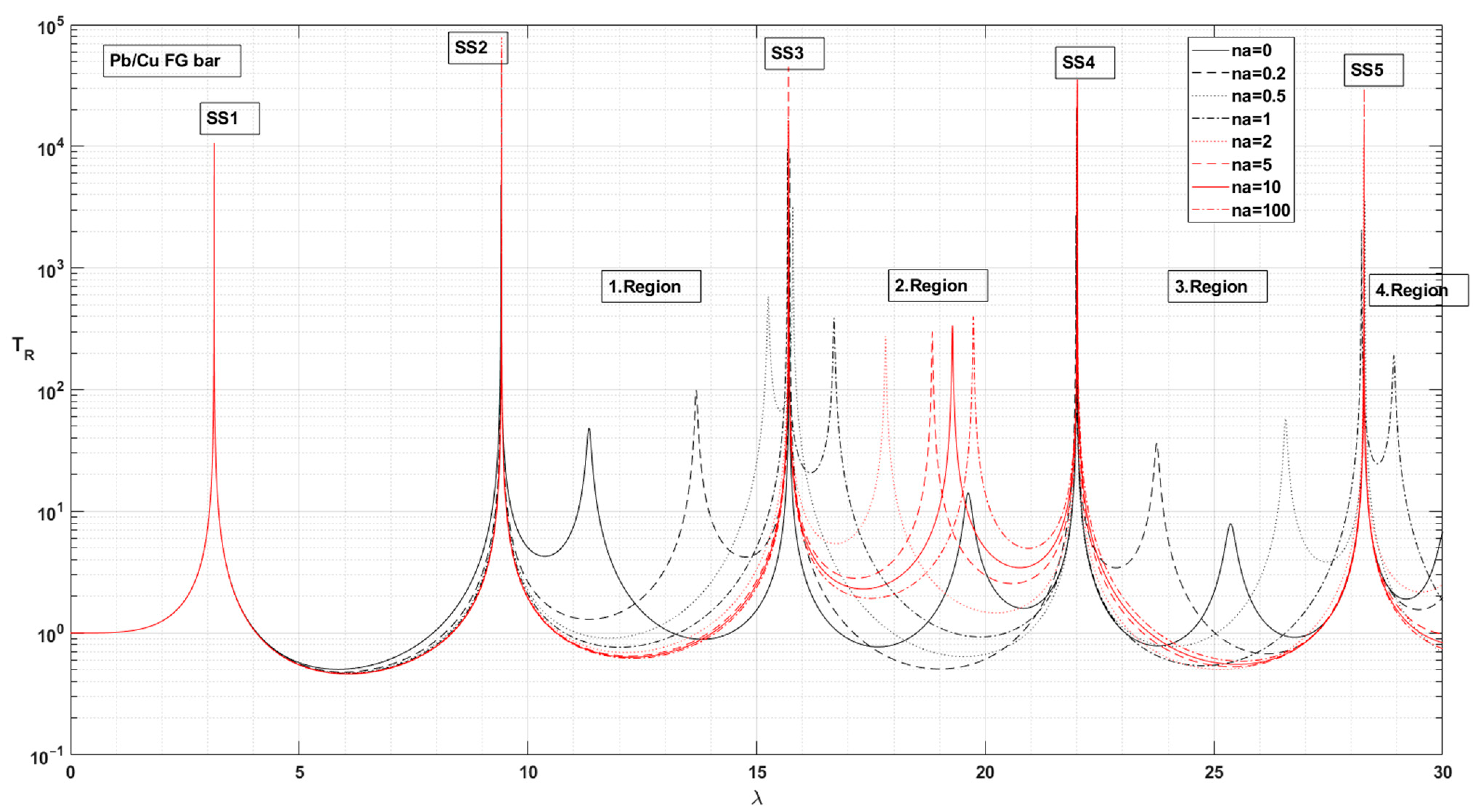
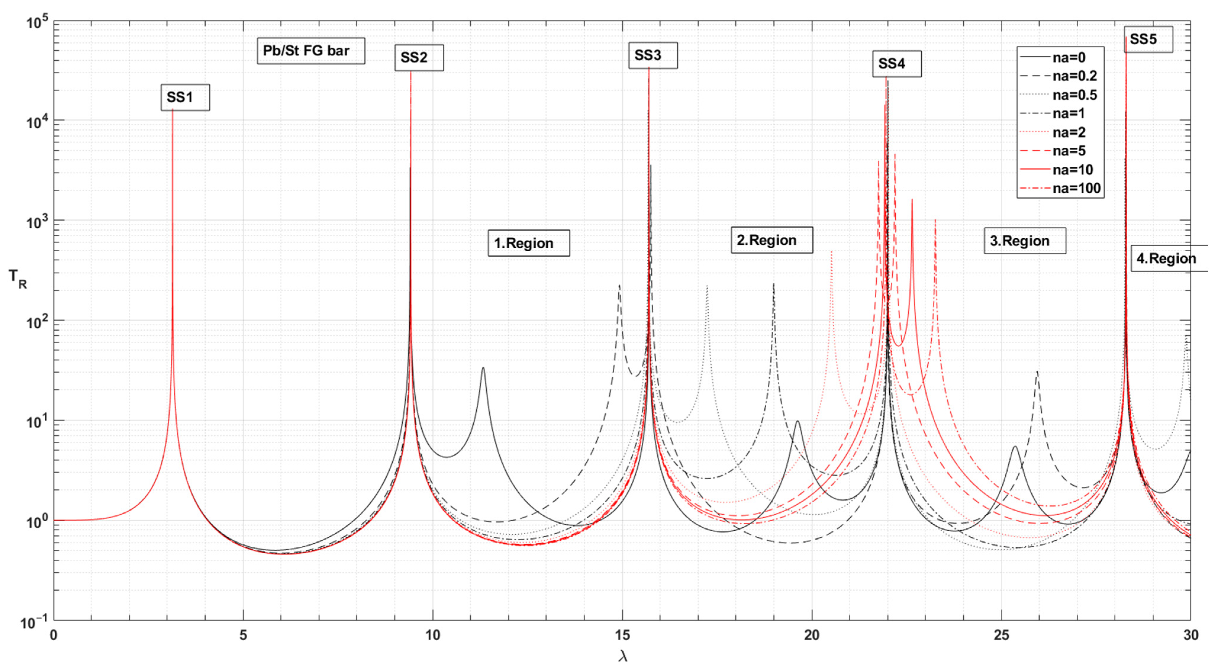
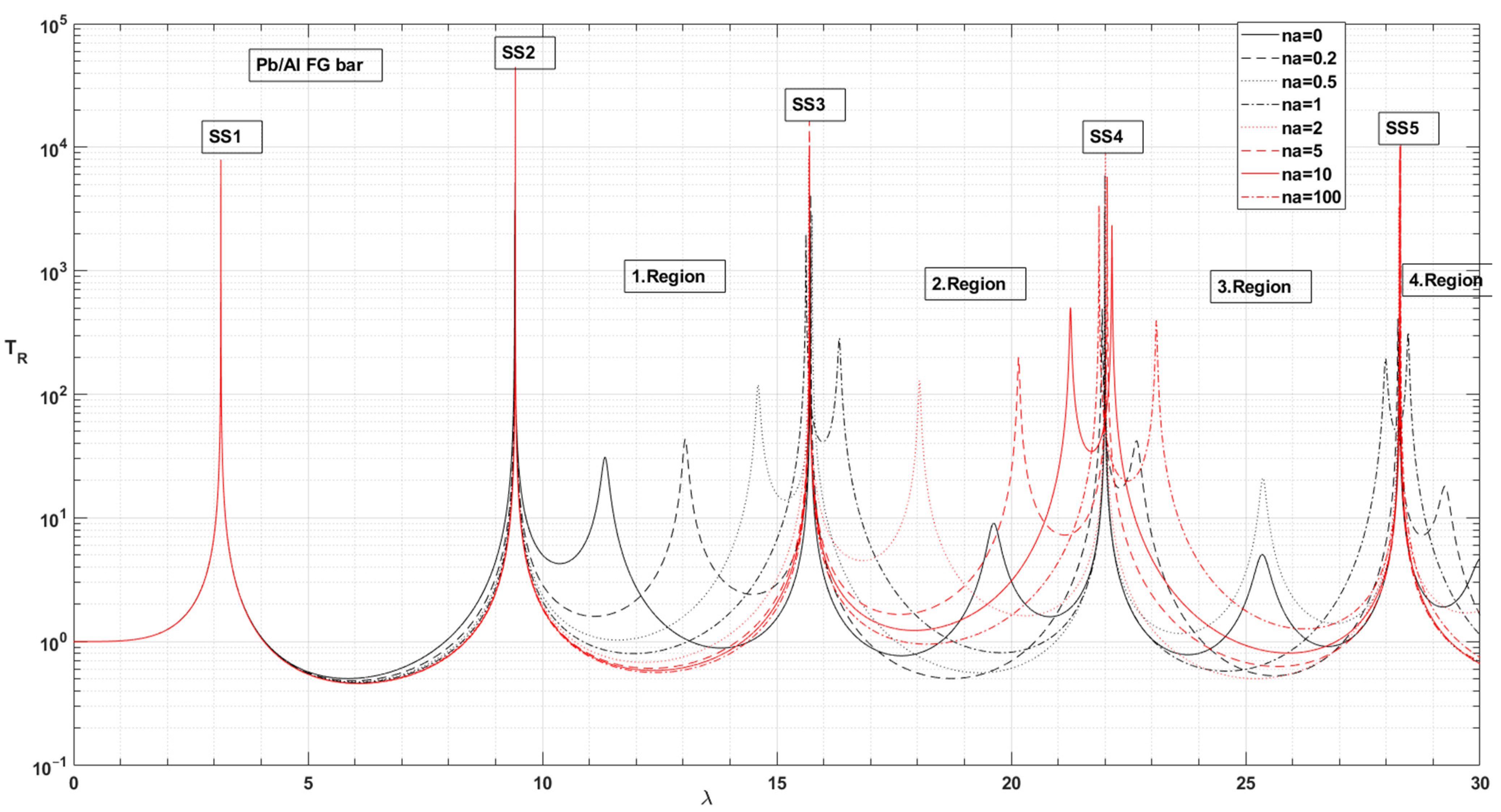
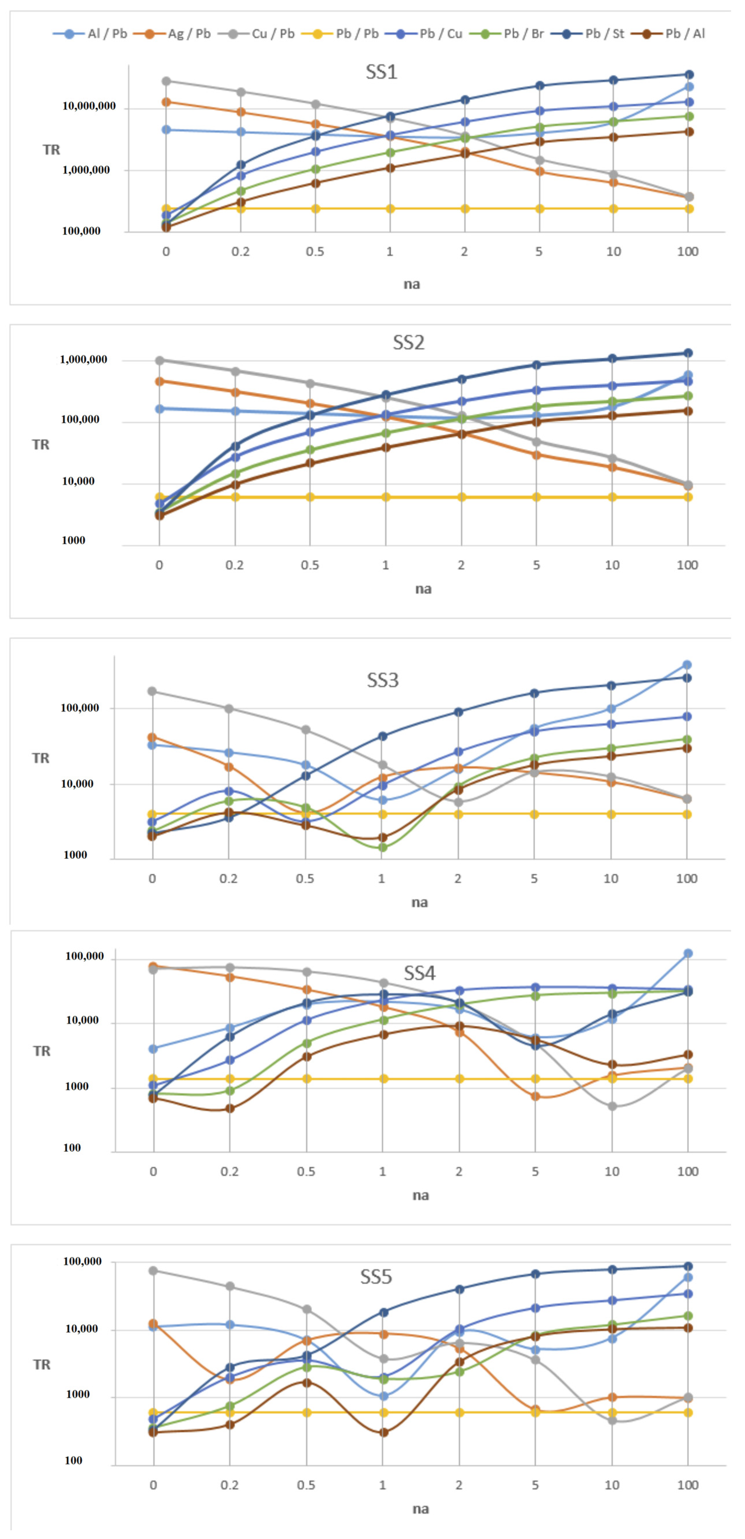
• For the system with the Pb/Cu, Pb/Br, Pb/St and Pb/Al support bars, c_Aratio > 1 and for the frequency parameters SS1 and SS2, the T_R force transmission values increase with increasing na. The values of the T_R force transmission decrease with increasing c_Aratio if c_Aratio > 1 (Figure 20 and Table 8).
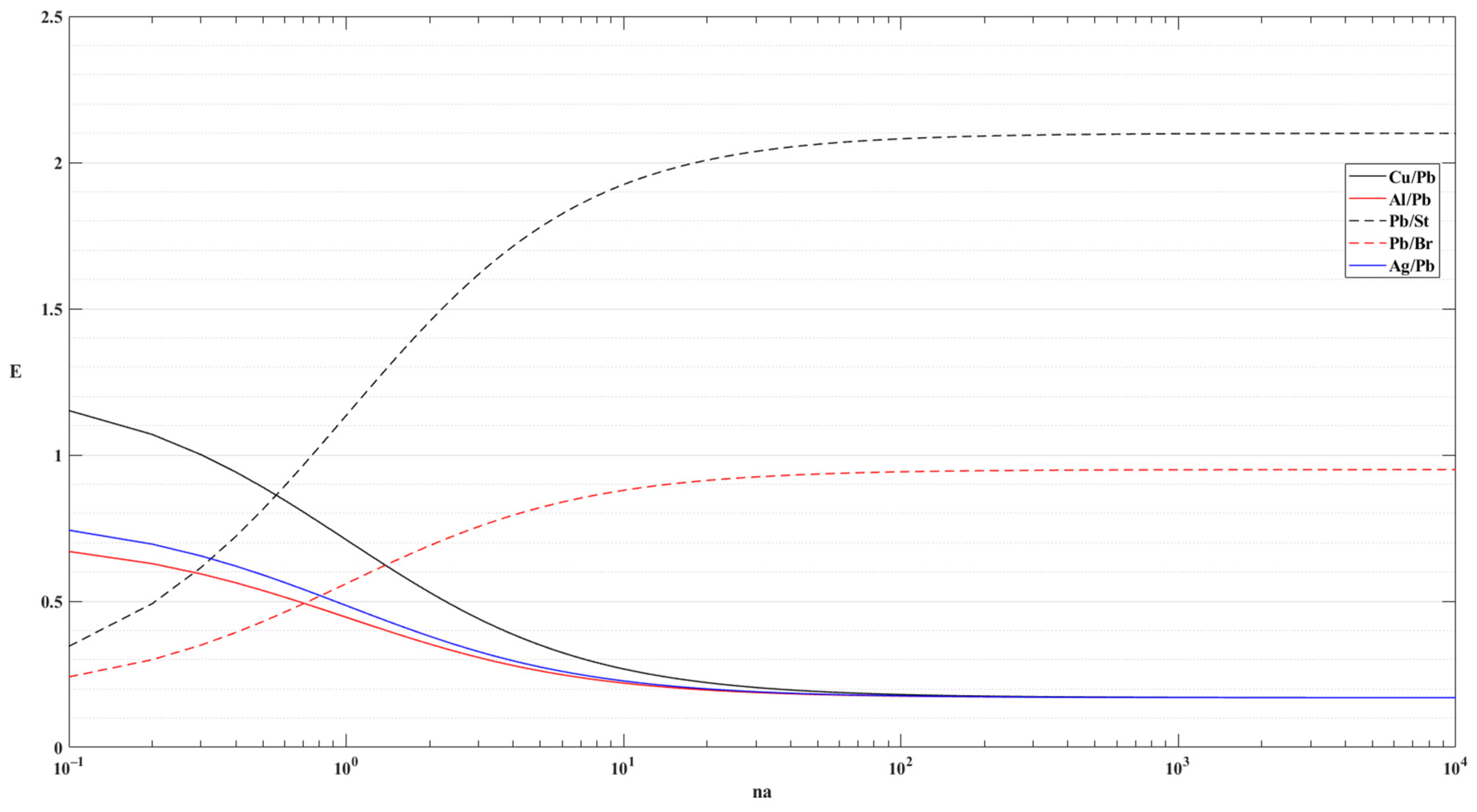
• In the frequency parameters SS1 and SS2, the bar material pairs with c_Aratio > 1 Pb/Cu, Pb/Br, Pb/St and Pb/Al are ranked in insulation quality as the na value increased towards 100. Excluding Pb/St, T_R is ranked according to the c_Aratio value (Table 5). It can be seen that the Eratio for the Pb/St pair is very low when other material pairs are considered (Table 5). The support bar made of the Pb/Al material pair with the highest c_Aratio value provides better insulation (Table 8, Figure 20).
• When c_Aratio > 1, the system with Pb/Al bars provides the best insulation for all values of na. On the other hand, when na = 0, although the bar material behaves like Pb, the insulation is better than the system supported by the pure Pb bar. The change in force transmissibility of the system using pure Pb bar supports is shown in Figure 3 and Table 3. Table 6 shows that for the frequency parameter SS1, the T_R value decreases from 243,782 in the Pb bar-supported system to 123,496 in the Pb/Al bar-supported system; for the frequency parameter SS2, the T_R value decreases from 6144 in the Pb supported system to 3108 in the Pb/Al supported system. The lowest T_R value of the frequency parameter SS1, na = 0, is 4,584,299 for the Al/Pb material pair bar-supported system. Whether the Pb material is at the bottom or the top affects the transmissibility (Table 7 and Table 8, Figure 20).
• For the system with the Al/Pb, Ag/Pb and Cu/Pb support bars, c_Aratio < 1, and for the frequency parameters SS1 and SS2, the T_R force transmission values decrease with increasing na. The values of the T_R force transmission increase with increasing c_Aratio if c_Aratio < 1 (Figure 20 and Table 6).
• In the frequency parameters SS1 and SS2, the bar material pairs with c_Aratio < 1 Al/Pb, Ag/Pb and Cu/Pb are ranked in terms of insulation quality as the na value increased towards 100 until the na = 1 value. Excluding Al/Pb, the T_R is ranked according to the c_Aratio value (Table 5). The T_R of the system with the Al/Pb bar material pair has a turning point at na = 2 and then increases. The support bar made of the Al/Pb and Ag/Pb material pairs with the lowest c_Aratio value provides better insulation for the different na regions (Table 6, Figure 20). When other material pairs are considered, it is seen that the c_Aratio is very low in the Pb/Al pair (Table 6).
• The T_R force transmission values decrease as the frequency parameters (SS1 compared with SS2, SS3, SS4, SS5) increase (Figure 20, Table 6, Table 7 and Table 8).
• For the frequency parameters SS1, SS2, SS3, SS4 and SS5 and for na = 0, T_R decreases with increasing c_Aratio if c_Aratio > 1, while T_R increases with increasing c_Aratio if c_Aratio < 1 (Table 6, Table 7 and Table 8).
• The T_R values of the system with the support bar consisting of c_Aratio > 1 material pairs at na = 100 are ranked according to Young’s modulus, except for the Al/Pb material pair (Figure 20, Table 8). The effect of the second material increases with increasing na in material pairs.
• For the SS frequency parameters of the system with the Ag/Pb and Cu/Pb material pairs under the condition of c_Aratio < 1, the T_R values are maximum for na = 0, while the T_R values are minimum for na = 100. Although there are exceptional cases, the general trend is in this direction. In contrast to the other material pairs with c_Aratio < 1, for the SS frequency parameters of the system with the Al/Pb material pair, the T_R values are maximum for na = 100, while the T_R values are minimum for na = 0 and the various na values (Table 6, Figure 20).
• When c_Aratio > 1, for SS frequencies, minimum T_R values are realised for na = 0 and maximum T_R values for na = 100. The minimum and maximum values are shown in Table 6 and Table 8 with different background colours (max: orange and min: green).
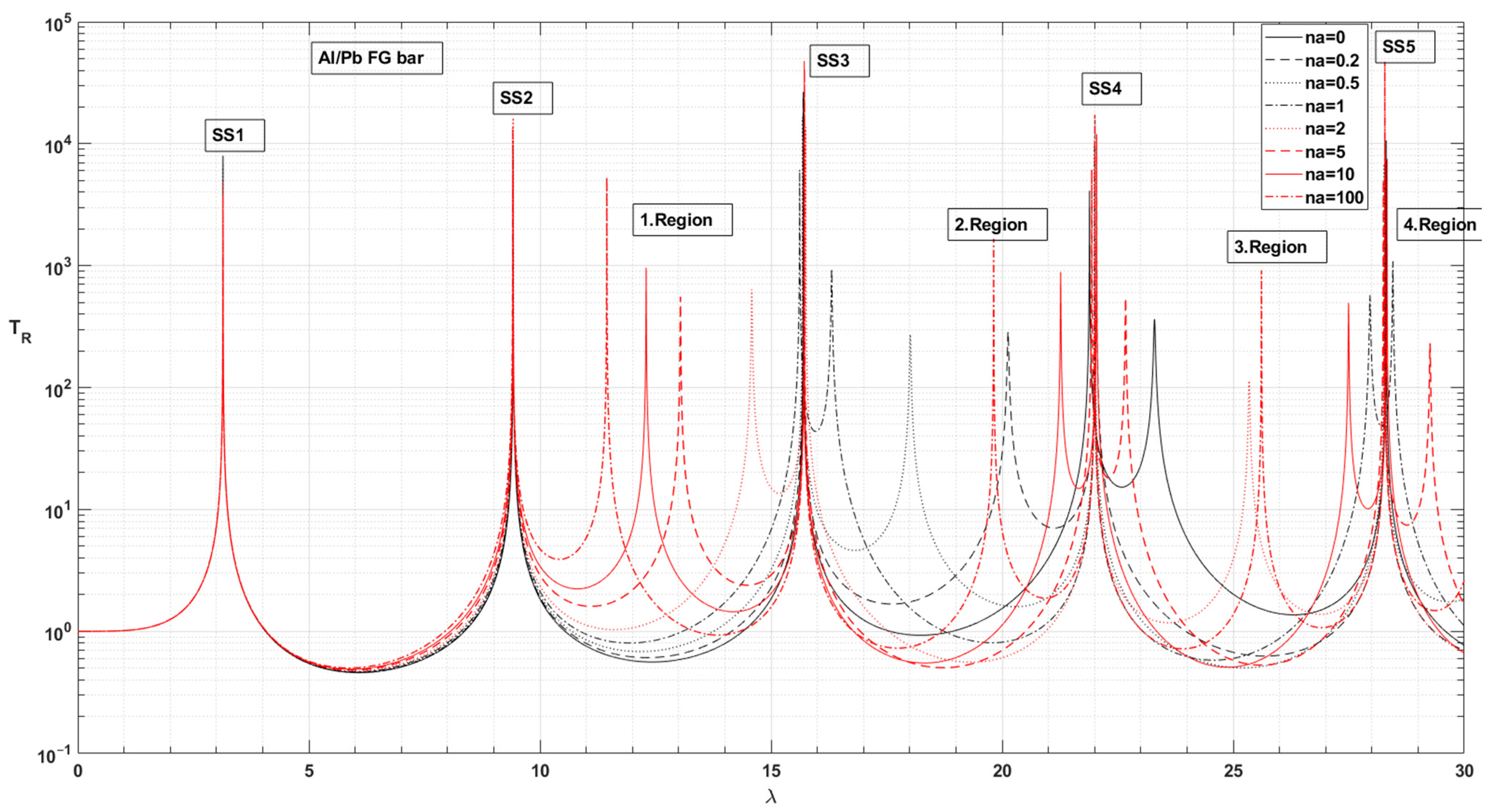
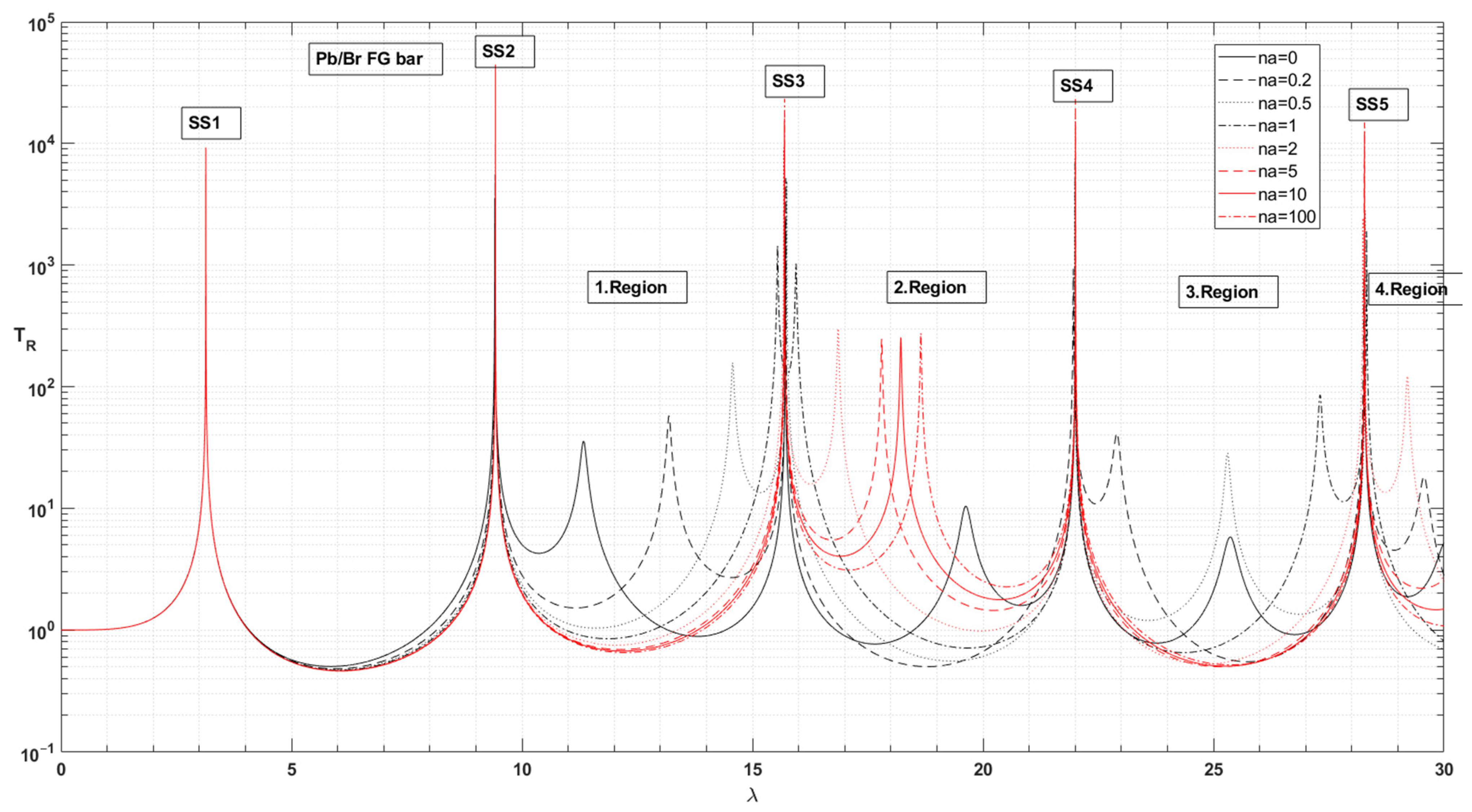
• In the frequency responses of SS3, SS4 and SS5, in the case of c_Aratio > 1, although the trend is for T_R to increase with increasing na, the trend has minima at different na values. The minimum values of T_R are lower than the value of pure Pb. In the case of c_Aratio < 1, except for the Al/Pb material pair, the decreasing T_R trend continues after making minima at different na values. For SS4 and SS5 frequency responses, the minimum values of T_R are lower than the values of pure Pb. For SS3, SS4 and SS5 frequency parameters, the best isolation of the force transmission is achieved at different na values. The material pairs and na values that provide better isolation than the pure Pb bar system are as follows:
  • SS3 frequency response: for Pb/Al, Pb/Br material pairs at na = 1 and Pb/Cu at na = 0.5, the best isolation is achieved with Pb/Br material at na = 0.5;
  • SS4 frequency response: for Pb/Al, Pb/Br material pairs at na = 0.2 and Ag/Pb material at na = 5 and for Cu/Pb material at na = 10 with minimum transmission, the best isolation is achieved with Pb/Al material pair at na = 0.2;
  • SS5 frequency response: with minimum transmission values of Pb/Al at na = 1 and Cu/Pb at na = 10, the best isolation is achieved with the material pair Pb/Al, na = 1 (Figure 20 and Table 6, Table 7 and Table 8).
• In the regions where the bar motion is dominant, 1.region and others, there is a minimum force transmission for na = 0 for the materials with c_Aratio > 1, while maximum T_R values occur for different values of na. For the materials with c_Aratio < 1, there is a minimum force transmission for na = 100 except for the Al/Pb material pair. There is a maximum force transmission for na = 100, while minimum T_R values occur for different values of na for the Al/Pb material pair (Table 6 and Table 8).
• In 1. Region, there is a trend for the transmissibility of the side frequency parameters. This distribution shows a trend according to na less than and greater than 1 for the other regions. For the material pairs with c_Aratio > 1 and Al/Pb material (c_Aratio < 1), T_R values increase with increasing na. For the material pairs with c_Aratio < 1, the T_R values decrease with increasing na (Table 6 and Table 8 and Figure 13, Figure 14, Figure 15, Figure 16, Figure 17, Figure 18 and Figure 19).
• The T_R values decrease as the frequency parameters increase for 1. Region, 2. Region and 3. Region for na = 100 and c_Aratio < 1 (i.e., T_R values, 1. Region: 5305, 2. Region: 1681, 3. Region: 919 for the Al/Pb material pair at na = 100 in Table 6). This trend occurs for maxima values for Al/Pb and the minima values for Ag/Pb and Cu/Pb material pairs (Table 6).
• The T_R values decrease as the frequency parameters increase in 1. Region, 2. Region and 3. Region for na = 0 and c_Aratio >1 (i.e., T_R values, 1. Region: 31, 2. Region: 9, 3. Region: 5 for the Pb/Al material pair at na = 0 in Table 8).
• The na values of material pairs that minimise force transmission in the side frequency regions can be written as follows:
  • Bar with Al/Pb material: 1. Region and before at na = 0, 2. Region at na = 5, 3. Region at na = 0.5;
  • Bar with Ag/Pb material: 1. Region and before na = 0, 2. Region na = 2, 3. Region na = 5;
  • Bar with Cu/Pb material; 1. Region and before na = 0, 2. Region na = 5, 3. Region na = 10;
  • Bar with Pb/Cu material: 1. Region and before na = 100, 2. Region na = 0.2, 3. Region na = 5;
  • Bar with Pb/Br material: 1. Region and before na = 100, 2. Region na = 0.2, 3. Region na = 10;
  • Bar with Pb/St material: 1. Region and before na = 100, 2. Region na = 0.2, 3. Region na = 0.5;
  • Bar with Pb/St material: 1. Region and before na = 100, 2. Region na = 0.2, 3. Region na = 2 (Figure 13, Figure 14, Figure 15, Figure 16, Figure 17, Figure 18 and Figure 19).

Taking into account the parameters na and c_Aratio, the investigations of Figure 13, Figure 14, Figure 15, Figure 16, Figure 17, Figure 18 and Figure 19, Figure 21 and Table 6, Table 7 and Table 8 for the frequency parameters λ can be grouped as follows:

17.

For the system with the Pb/Cu, Pb/Br, Pb/St and Pb/Al support bars, c_Aratio > 1, the frequency parameters SS1 and SS2 decrease with increasing na. The values of the frequency parameters increase with increasing c_Aratio if c_Aratio < 1 (Figure 21 and Table 8).

18.

For the system with the Al/Pb, Ag/Pb and Cu/Pb support bars, c_Aratio < 1, the frequency parameters decrease with increasing na in the 1. Region (Table 6). The contrast in T_R force transmission (T_R) between material pairs with c_Aratio < 1 is not seen here. This situation appears to be the effect of material damping and Young’s modulus.

19.

For the system with the Al/Pb, Ag/Pb0 and Cu/Pb support bars, c_Aratio < 1, the frequency parameters increase with increasing na in the 1. Region (Figure 13, Figure 14, Figure 15, Figure 16, Figure 17, Figure 18, Figure 19 and Figure 21 and Table 6).

20.

In 1. Region, for the system with bars of Pb/Cu, Pb/Br, Pb/St and Pb/Al material pairs, c_Aratio > 1, the frequency parameters increase with increasing na (Table 8).

21.

There is a trend for the values of the side frequency parameters in the other regions. This distribution shows a trend according to na less than and greater than 1 (Figure 13, Figure 14, Figure 15, Figure 16, Figure 17, Figure 18, Figure 19 and Figure 21 and Table 6, Table 7 and Table 8).

22.

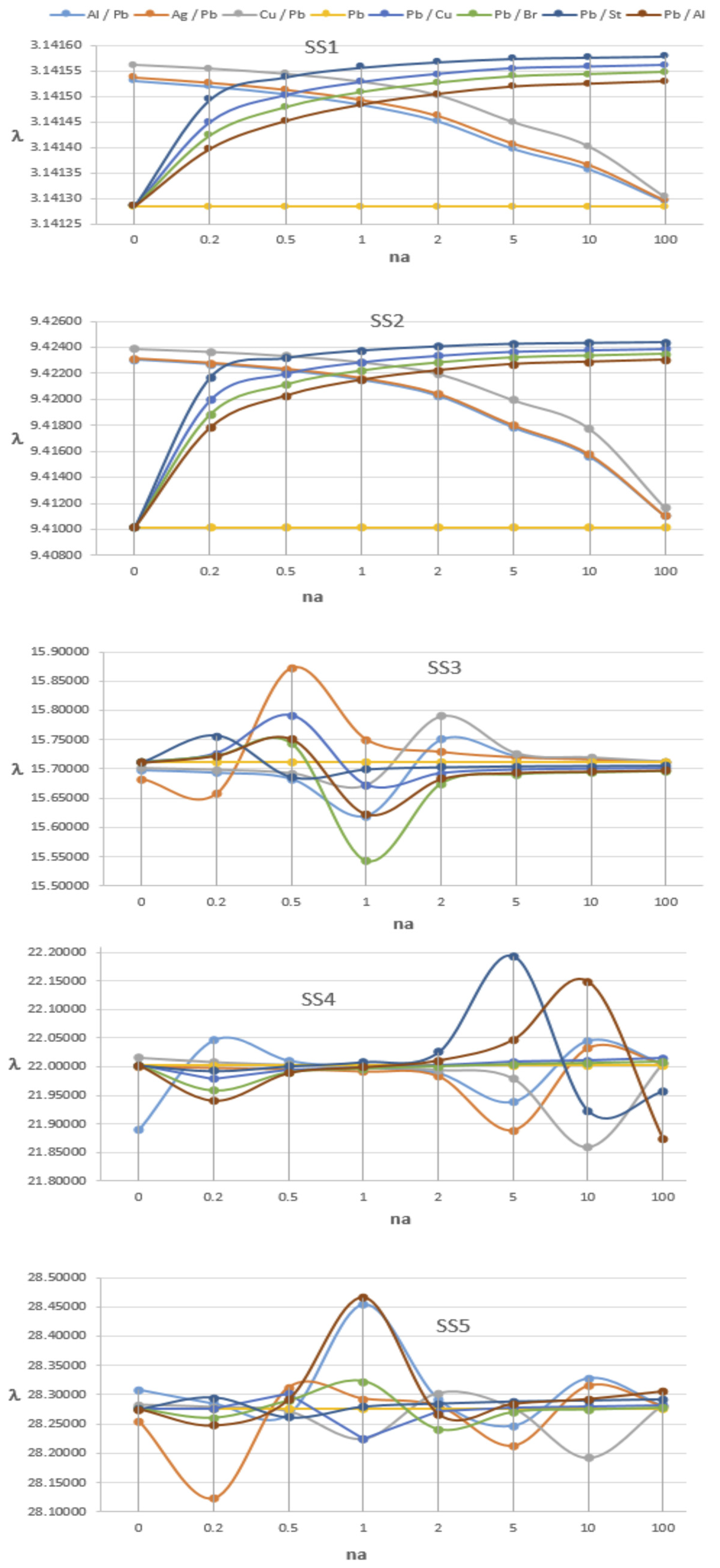
The side frequencies show an ordered distribution as a function of na over 0–30 Hz. In other frequency ranges, as the bar begins to dominate the overall motion, it is difficult to see a trend due to the dependence of the frequency parameters on specific mass and Young’s modulus. Although there are approaches in the literature to overcome this situation by considering the specific mass ratio as 1, in this study, since beam isolation is the main concern, real material properties are used for the bar. However, the graph for SS3 in Figure 21 shows that the frequency parameters remain constant when na > 5, whereas the graph for SS4 shows that the frequency parameters remain constant in the range 0.5 < na < 2 (Figure 13, Figure 14, Figure 15, Figure 16, Figure 17, Figure 18, Figure 19 and Figure 21 and Table 6, Table 7 and Table 8).

23.

Since it is possible to influence the elasticity and mass distribution with na, isolation in the form of a dynamic absorber will be possible for the relevant frequency. While the peak value is minimised at a certain frequency, the frequency is decomposed as two different peak values. This may be a different approach to the study of minimising the vibration made by Mi and Song [28]. As an example of this situation, Figure 13, Figure 15, Figure 17 and Figure 18 show that for the material pair Al/Pb, SS3 and SS5 for na = 1; for the material pair Cu/Pb, SS5 for na = 10; for the material pair Pb/Br, SS3 for na = 1; and for the material pair Pb/St, SS4 frequency can be given as na = 5.

7. Conclusions

The harmonic response of a beam supported at the ends with the FG viscoelastic bars is considered. The harmonic force is applied at the centre of the beam. The FG viscoelastic bars are connected to the end points of a beam by rotary joints to ensure that they work only in the axial direction. The effects of the length-varying material properties and internal damping of the FG bars on the force transmission T_R and frequency parameters λ are examined in detail. No study has been found in the literature on the vibration of FG viscoelastic bar-supported beams subjected to a harmonic force at the centre point. The functional variation of the internal damping property between two different materials is defined depending on the Young’s modulus and material damping. This study show that the longitudinally varying bar properties and the longitudinally varying internal damping coefficient are very effective on the dynamic behaviour of the beam.

In the light of all the findings, the following observations can be made.

It is seen that the longitudinal variation of the internal damping significantly reduces the responses compared to the normal internal damping which is naturally present in all materials. By selecting the appropriate material distribution with material distribution coefficient, better force transmission can be achieved from the pure material. The internal damping effect varies according to whether the vibration mode is bar-dominated or beam-dominated for the bar-supported beam.

The internal damping ratio of the viscoelastic support bar has a significant effect on insulation. This is achieved by increasing the ratio for ratio > 1 and by decreasing the ratio for ratio < 1. The force transmission values are lower when ratio > 1 than when ratio < 1. The force transmission ratio (T_R) is lower when the part pressing on the ground has a larger internal damping. The transmission of force in bars with the material pairs Al/Pb and Pb/Al is an example of this situation. Between material pairs (as in the case of Pb/St and Al/Pb pairs), the force transfer characteristics change as the ratio of Young’s modulus and internal damping coefficient closes to zero.

By controlling the values of the internal damping ratio and material distribution coefficient of the bar, the system’s frequency parameters can be increased or decreased, or a constant value can be maintained within certain ranges at high frequencies. The frequency parameters can remain nearly constant locally despite the changing value of the material distribution coefficient value.

The frequency parameters generally increase with the increase in bar area. However, this situation is reversed after the bar effect is seen as a frequency parameter in the system.

The effect of the bar area on force transmission depends on the vibration mode. The force transmission decreases with the increase in the bar area for the bar-dominant vibration mode. The force transmission gives minima at different area values for the beam dominant vibration mode.

Experimental studies on material damping indicate that the damping is independent of velocity and increases in proportion to the square of the displacement. Therefore, in the case of material-dependent damping, the damping occurs at the same frequency. In the AFG viscoelastic bar, the effect of the material damping change is considered together with the specific mass and Young’s modulus. The effect of material damping, which is only seen as a change in amplitude at the same frequency, begins to change based on frequencies.

It is possible to minimise the force transmission for a certain frequency parameter by adjusting the stiffness, mass and internal damping distribution with the material coefficient in the frame of dynamic absorber logic.

In future studies, the application of viscoelastic FG bars to functionally graded beams can be investigated. The ratios of the material change coefficients of two FG structures in isolation can provide important practical data. The internal damping is defined for the FG bending element. The internal damping varies exponentially throughout its thickness. The dynamic behaviour and vibration isolation can be investigated for the system. Although not analysed here for the sake of brevity, for each material pair and damping value, an optimum material change coefficient na and internal material damping coefficient c_A can be found to minimise the dynamic response of the beam.

In conclusion, when a FG viscoelastic bar is used as a support element, the mass distribution, stiffness and internal damping distribution can be controlled by using the material distribution coefficient. Thus, the isolation can be performed better.

References

1. Fan, Z.-J.; Lee, J.-H.; Kang, K.-H.; Kim, K.-J. The Forced Vibration Of A Beam with Viscoelastic Boundary Supports. J. Sound Vib. 1998, 210, 673–682. [Google Scholar] [CrossRef]
2. Jacquot, R.G. Optimal Damper Location for Randomly Forced Cantilever Beams. J. Sound Vib. 2004, 269, 623–632. [Google Scholar] [CrossRef]
3. Abu-Hilal, M.; Mohsen, M. Vibration Of Beams with General Boundary Conditions Due To A Moving Harmonic Load. J. Sound Vib. 2000, 232, 703–717. [Google Scholar] [CrossRef]
4. Wang, D.; Wen, M. Vibration Attenuation of Beam Structure with Intermediate Support under Harmonic Excitation. J. Sound Vib. 2022, 532, 117008. [Google Scholar] [CrossRef]
5. Jacquot, R.G. Random Vıbratıon of Damped Modıfıed Beam Systems. J. Sound Vib. 2000, 234, 441–454. [Google Scholar] [CrossRef]
6. Jacquot, R.G. The Spatial Average Mean Square Motion as an Objective Function for Optimizing Damping in Damped Modified Systems. J. Sound Vib. 2003, 259, 955–965. [Google Scholar] [CrossRef]
7. Baz, A.M. Active and Passive Vibration Damping; John Wiley & Sons Ltd: Oxford, UK, 2018; pp. 1–55. [Google Scholar]
8. Cremer, L.; Heckl, M.; Petersson, B.A.T. Structure-Borne Sound, 3rd ed.; Springer: Berlin/Heidelberg, Germany, 2005; pp. 149–232. [Google Scholar]
9. He, J.; Fu, Z.F. Modal Analysis; Butterworth-Heinemann: Oxford, UK, 2001; pp. 123–139. [Google Scholar]
10. Petyt, M. Introduction to Finite Element Vibration Analysis, 2nd ed.; Cambridge University Press: Cambridge, UK, 2010; pp. 352–355. [Google Scholar]
11. Rao, S.S. Mechanical Vibrations, 5th ed.; Pearson: London, UK, 2004; pp. 192–197. [Google Scholar]
12. Maia, N. Reflections on the Hysteretic Damping Model. Shock. Vib. 2009, 16, 529–542. [Google Scholar] [CrossRef]
13. Lisitano, D.; Slavič, J.; Bonisoli, E.; Boltežar, M. Strain Proportional Damping in Bernoulli-Euler Beam Theory. Mech. Syst. Signal Process 2020, 145, 106907. [Google Scholar] [CrossRef]
14. Pan, D.; Fu, X.; Qi, W. The Direct Integration Method with Virtual Initial Conditions on the Free and Forced Vibration of a System with Hysteretic Damping. Appl. Sci. 2019, 9, 3707. [Google Scholar] [CrossRef]
15. Tsai, T.-C.; Tsau, J.-H.; Chen, C.-S. Vibration Analysis of a Beam with Partially Distributed Internal Viscous Damping. Int. J. Mech. Sci. 2009, 51, 907–914. [Google Scholar] [CrossRef]
16. Chen, W.-R. Bending Vibration of Axially Loaded Timoshenko Beams with Locally Distributed Kelvin–Voigt Damping. J. Sound Vib. 2011, 330, 3040–3056. [Google Scholar] [CrossRef]
17. Kocatürk, T.; Şimşek, M. Vibration of Viscoelastic Beams Subjected to an Eccentric Compressive Force and a Concentrated Moving Harmonic Force. J. Sound Vib. 2006, 291, 302–322. [Google Scholar] [CrossRef]
18. Freundlich, J. Transient Vibrations of a Fractional Kelvin-Voigt Viscoelastic Cantilever Beam with a Tip Mass and Subjected to a Base Excitation. J. Sound Vib. 2019, 438, 99–115. [Google Scholar] [CrossRef]
19. Chen, W.-R. Parametric studies on bending vibration of axially-loaded twisted Timoshenko beams with locally distributed Kelvin–Voigt damping. Int. J. Mech. Sci. 2014, 88, 61–70. [Google Scholar] [CrossRef]
20. Sepehri-Amin, S.; Faal, R.T.; Das, R. Analytical and Numerical Solutions for Vibration of a Functionally Graded Beam with Multiple Fractionally Damped Absorbers. Thin-Walled Struct. 2020, 157, 106711. [Google Scholar] [CrossRef]
21. Demir, C.; Oz, F.E. Free Vibration Analysis of a Functionally Graded Viscoelastic Supported Beam. J. Vib. Control 2013, 20, 2464–2486. [Google Scholar] [CrossRef]
22. Deng, H.; Chen, K.; Cheng, W.; Zhao, S. Vibration and Buckling Analysis of Double-Functionally Graded Timoshenko Beam System on Winkler-Pasternak Elastic Foundation. Comp. Struct. 2017, 160, 152–168. [Google Scholar] [CrossRef]
23. Duy, H.T.; Van, T.N.; Noh, H.C. Eigen Analysis of Functionally Graded Beams with Variable Cross-Section Resting on Elastic Supports and Elastic Foundation. Struct. Eng. Mech. 2014, 52, 1033–1049. [Google Scholar] [CrossRef]
24. Akbaş, Ş.D.; Fageehi, Y.A.; Assie, A.E.; Eltaher, M.A. Dynamic Analysis of Viscoelastic Functionally Graded Porous Thick Beams under Pulse Load. Eng. Comput. 2020, 38, 365–377. [Google Scholar] [CrossRef]
25. Nikolić, A. Free Vibration Analysis of a Non-Uniform Axially Functionally Graded Cantilever Beam with a Tip Body. Arch. Appl. Mech. 2017, 87, 1227–1241. [Google Scholar] [CrossRef]
26. Huang, Y.; Rong, H.-W. Free Vibration of Axially Inhomogeneous Beams That Are Made of Functionally Graded Materials. Int. J. Acoust. Vib. 2017, 22, 68–73. [Google Scholar] [CrossRef]
27. Demir, E.; Sayer, M.; Callioglu, H. An Approach for Predicting Longitudinal Free Vibration of Axially Functionally Graded Bar by Artificial Neural Network. Proc. Inst. Mech. Eng. Part C J. Mech. Eng. Sci. 2022, 237, 2245–2255. [Google Scholar] [CrossRef]
28. Mi, X.; Song, Z. A Mode Localization Inspired Vibration Control Method Based on the Axially Functionally Graded Design for Beam Structures. Comp. Struct. 2024, 343, 118300. [Google Scholar] [CrossRef]
29. Demir, C. Natural Frequencies of a Viscoelastic Supported Axially Functionally Graded Bar with Tip Masses. Int. J. Acoust. Vib. 2023, 28, 50–64. [Google Scholar] [CrossRef]
Figure 1. A beam supported with axially functional graded viscoelastic bars.
Applsci 14 08974 g001
Figure 2. A two-node finite element bar model in local coordinate system.
Applsci 14 08974 g002
Figure 3. A finite element with two nodes for the beam in the local coordinate system.
Applsci 14 08974 g003
Figure 4. Degrees of freedom used for beam and bar assembly in global coordinate system.
Applsci 14 08974 g004
Figure 5. The force transmissibility of the isotropic steel beam supported with rigid bars.
Applsci 14 08974 g005
Figure 6. Boundary conditions of the system for the finite element model of Ansys Workbench.
Applsci 14 08974 g006
Figure 7. The harmonic response of steel beam with supported rigid alumina bar (E = 70 × 1080 N/m2) and reaction force in frequency domain.
Applsci 14 08974 g007
Figure 8. The changing area effects on the force transmissibility of the steel beam supported by lead bars.
Applsci 14 08974 g008
Figure 9. The changing area effects on the force transmissibility of the steel beam supported by aluminium bars.
Applsci 14 08974 g009
Figure 10. Force transmissibility of the lead supported beam with material damping.
Applsci 14 08974 g010
Figure 11. The effect of various bar materials on the force transmissibility of the system.
Applsci 14 08974 g011
Figure 12. Young’s modulus changes depending on the material change coefficient “na” for the different material pairs.
Applsci 14 08974 g012
Figure 13. Force transmissibility of axial FG viscoelastic Al-Pb bar supported steel beam according to material change coefficient na.
Applsci 14 08974 g013
Figure 14. Force transmissibility of axial FG viscoelastic Ag-Pb bar supported steel beam according to material change coefficient na.
Applsci 14 08974 g014
Figure 15. Force transmissibility of axial FG viscoelastic Cu-Pb bar supported steel beam according to material change coefficient na.
Applsci 14 08974 g015
Figure 16. Force transmissibility of axial FG viscoelastic Pb-Cu bar supported steel beam according to material change coefficient na.
Applsci 14 08974 g016
Figure 17. Force transmissibility of axial FG viscoelastic Pb-Br bar supported steel beam according to material change coefficient na.
Applsci 14 08974 g017
Figure 18. Force transmissibility of axial FG viscoelastic Pb-St bar supported steel beam according to material change coefficient na.
Applsci 14 08974 g018
Figure 19. Force transmissibility of axial FG viscoelastic Pb-Al bar supported steel beam according to material change coefficient na.
Applsci 14 08974 g019
Figure 20. Variation of system force transmission concerning material change coefficients at vibration modes SS1, SS2, SS3, SS4 and SS5 for support bars in different material pairs.
Applsci 14 08974 g020
Figure 21. Variation of system frequency parameters concerning material change coefficients at vibration modes SS1, SS2, SS3, SS4 and SS5 for support bars in different material pairs.
Applsci 14 08974 g021