Three-Dimensional MT Conductive Anisotropic and Magnetic Modeling Using A − ϕ Potentials Employing a Mixed Nodal and Edge-Based Element Method

Abstract

Magnetotelluric (MT) sounding is a geophysical technique widely utilized in mineral resource surveys, where conductivity and magnetic permeability serve as essential physical parameters for forward modeling and inversion. However, the effects of conductive anisotropy and non-zero magnetic susceptibility are usually ignored. In this study, we present a three-dimensional (3D) MT modeling algorithm using Coulomb-gauged electromagnetic potentials, incorporating a mixed nodal and edge-based finite element method capable of simulating MT responses for conductive anisotropic and magnetic anomalies. Subsequently, the algorithm’s accuracy was validated in two steps: first, it was compared with analytical solutions for a 1D magnetic model; then, a comparison was made with previously published numerical results for a 3D generalized conductive anisotropic model. The results of two tests show that the maximum relative error is below 0.5% for both models. Furthermore, representative models were computed to comprehensively analyze the responses of MT. The findings illustrate the relationship between anisotropic parameters and electric fields and emphasize the significance of considering the impact of magnetic susceptibility in magnetite-rich regions.

1. Introduction

Magnetotelluric (MT) sounding is a crucial technique widely employed in applied geophysics, e.g., for mineral resource surveys [1,2]. The commonly used numerical modeling techniques for MT modeling include the finite difference method (FDM) [3], the finite-element method (FEM) [4], and the integral equation method [5]. On the other hand, apart from deriving governing equations directly for either the electric field or the magnetic field, another popular approach involves decomposing the Helmholtz equation into the electric scalar potential $\varphi$ and the magnetic vector potential $\mathbf{A}$ under the Coulomb-gauged condition $\nabla \cdot \mathbf{A}=0$ [6,7]. This approach is also known as the $\mathbf{A}-\varphi$ method [8].

Conductivity and magnetic permeability are two crucial physical parameters in MT forward modeling and inversion, and the phenomena of conductive anisotropy and non-zero susceptibility are commonly observed on the Earth [9,10]. Ignoring the influences of conductive anisotropy or magnetic susceptibility may result in misinterpretations of MT data [11,12]. Extensive research has been conducted on the forward modeling of MT in conductive anisotropic media [13,14]. Notably, Li [15] presented a node-based FEM for MT modeling in three-dimensional (3D) generalized anisotropic media, while the nodal FE method for MT modeling lacks accuracy due to the limitations regarding simulating electric fields at electrical interfaces. Löwer and Junge [16] investigated the spatial and frequency-dependent behavior of phase tensors and tipper vectors above a simple 3D anisotropic conductive anomaly using COMSOL MultiphysicsTM 4.3. Xiao et al. [17] proposed an algorithm utilizing an edge-based FEM to model 3D MT responses in arbitrary conductive anisotropic media, leading to insightful findings from their analysis of typical models. Kong et al. [14] conducted qualitative and quantitative analyses on 3D synthetic models using the staggered-grid FDM. Liu et al. [18] developed a 3D adaptive FEM that facilitates the simulation of irregular anomalies and topographies. Furthermore, Zhou et al. [19] introduced an FEM incorporating a divergence scheme specifically designed for axial conductive anisotropic media.

However, research concerning forward modeling in 3D conductive anisotropic and magnetic media remains limited, with only a few studies addressing this topic, to the best of our knowledge. Xiao et al. [20] proposed a method that directly operates on the electric field, while Yu et al. [9] presented an algorithm utilizing potentials through nodal FEM. In comparison to the results for the nodal FEM, the mixed nodal and edge-based FEM approach generates fewer unknowns, thereby enhancing computational efficiency. Therefore, we developed an alternative algorithm for MT modeling. In this study, we formulated the forward modeling of 3D MT in conductive anisotropic and magnetic media using $\mathbf{A}$ and $\varphi$ potentials employing the mixed nodal and edge-based FEM approach. This novel method offers distinct advantages for investigating the effects of conductive anisotropic and magnetic anomalies.

The paper is structured as follows: First, we present a comprehensive description of the mixed nodal and edge-based element method for 3D MT modeling based on Coulomb-gauged potentials. Next, we compare the numerical solution obtained from the algorithm with both the analytical solution of a 1D anisotropic model and the results derived from a 3D generalized anisotropic model to validate its accuracy. Finally, we conduct in-depth investigations on several representative models, exploring the impact of conductivity in different directions on the horizontal electric field and examining how magnetic permeability influences regions abundant in magnetite.

2. Methods

In this section, we present the modeling theory for 3D MT using the nodal and edge-based FE method, considering conductive anisotropic and magnetic anomalies. To the best of our knowledge, there is currently no relevant literature that simultaneously addresses both conductive anisotropic and magnetic anomalies using this algorithm.

2.1. A − ϕ Formulations

Displacement currents can be considered negligible at the frequencies employed in MT. The EM fields, characterized by a time dependence of ${\mathrm{e}}^{-i\omega t}$, are governed by the Maxwell’s differential equations, as follows,

$$\nabla \times \mathbf{E}=i\omega \mu \mathbf{H}$$

(1)

$$\nabla \times \mathbf{H}=\tilde{\sigma }\mathbf{E}.$$

(2)

where $\omega$ is the angular frequency, $\mu$ represents the magnetic permeability, $\mathbf{E}$ denotes the electric field, $\mathbf{H}$ is the magnetic field, and $\tilde{\sigma }$ is the symmetric tensor conductivity of the medium, as follows:

$$\tilde{\sigma }=\left(\begin{array}{ccc}{\sigma }_{xx}& {\sigma }_{xy}& {\sigma }_{xz}\\ {\sigma }_{yx}& {\sigma }_{yy}& {\sigma }_{yz}\\ {\sigma }_{zx}& {\sigma }_{zy}& {\sigma }_{zz}\end{array}\right).$$

(3)

where $\tilde{\sigma }$ is defined by six variables, namely, three principal conductivities (i.e., ${\sigma }_x$, ${\sigma }_y$, and ${\sigma }_z$) and three Euler angles (i.e., ${\alpha }_S$, ${\alpha }_D$, and ${\alpha }_L$) (see Reference [13] for details).

The EM field ($\mathbf{E}$,$\mathbf{H}$) can be expressed in terms of an electric scalar potential $\varphi$ and a magnetic vector potential $\mathbf{A}$, as follows:

$$\mathbf{B}=\nabla \times \mathbf{A},$$

(4)

$$\mathbf{E}=i\omega (\mathbf{A}+\nabla \varphi )$$

(5)

where $\mathbf{B}=\mu \mathbf{H}={\mu }_0{\mu }_r\mathbf{H}$, ${\mu }_r$ is the relative permeability, and ${\mu }_0$ is the magnetic permeability of free space.

Considering the Coulomb-gauged condition $\nabla \cdot \mathbf{A}=0$, Equations (6) and (7) can be obtained [6,7], as follows:

$$\nabla \times {\displaystyle \frac{\nabla \times \mathbf{A}}{\mu }}-i\omega \tilde{\sigma }(\mathbf{A}+\nabla \varphi )=0$$

(6)

$$\nabla \cdot \left[i\omega \tilde{\sigma }\right(\mathbf{A}+\nabla \varphi \left)\right]=0.$$

(7)

To maintain the symmetry of the stiffness matrix and to reduce adverse conditions, Equation (6) and Equation (7) are replaced by Equation (8) and Equation (9), respectively, as follows:

$$\nabla \times {\displaystyle \frac{\nabla \times \mathbf{A}}{{\mu }_r}}-i\omega {\mu }_0\tilde{\sigma }(\mathbf{A}+\nabla \varphi )=0,$$

(8)

$$\nabla \cdot [-i\omega {\mu }_0\tilde{\sigma }(\mathbf{A}+\nabla \varphi \left)\right]=0.$$

(9)

2.2. Boundary Conditions

Assuming that the boundaries of the problem domain are located sufficiently far from the anomalies, where the influences of the anomalies become negligible, Dirichlet boundary conditions are imposed on the outer boundary. Therefore,

$${\left.\varphi \right|}_{\mathsf{\Gamma }}=0$$

(10)

and

$${\left.\mathbf{A}\right|}_{\mathsf{\Gamma }}={\displaystyle \frac{{\left.\mathbf{E}\right|}_{\mathsf{\Gamma }}}{i\omega }}$$

(11)

where $\mathsf{\Gamma }$ denotes the outer boundaries of the entire study domain. Two orthogonal sources are located on the top surface of the problem domain, as follows: ${\mathrm{S}}_{\mathrm{A}}:({\mathrm{E}}_{\mathrm{x}},{\mathrm{E}}_{\mathrm{y}},{\mathrm{E}}_{\mathrm{z}})=(\mathrm{0,1},0)$ and ${\mathrm{S}}_{\mathrm{B}}:({\mathrm{E}}_{\mathrm{x}},{\mathrm{E}}_{\mathrm{y}},{\mathrm{E}}_{\mathrm{z}})=(\mathrm{1,0},0)$, respectively. ${\left.\mathbf{E}\right|}_{\mathsf{\Gamma }}$ is the solution for the two sources for the model without any 2D or 3D anomalies.

2.3. Finite Element Method Analysis

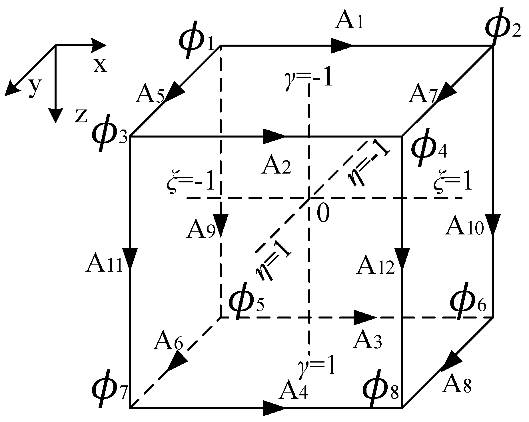
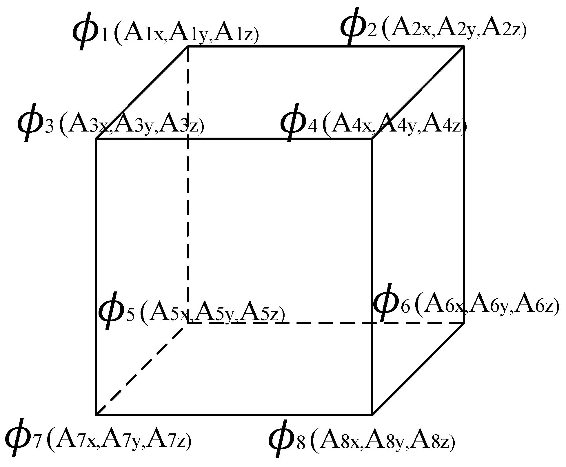
2.3.1. Mixed Nodal and Edge-Based Elements

The study domain is discretized using hexahedral elements, adopting mixed nodal and edge-based elements, as illustrated in Figure 1. The coordinates of the element’s center are denoted as ($X_0$, $Y_0$, $Z_0$), while the side lengths of the elements are represented by a, b, and c in the x-, y-, and z-directions, respectively.

The value of $\varphi$ is assigned as a constant at each node, while the values of $\mathbf{A}$ (i.e., $A_x$, $A_y$, and $A_z$) are assigned as constants along each edge. Therefore, for a given element, the constants $\mathbf{A}$ and $\varphi$ can be expressed as follows:

$${\mathbf{A}}_{\mathrm{e}}={\sum }_{\mathrm{i}=1}^4\left(N_{\mathrm{e}}^{\mathrm{x}\mathrm{i}}{A}_{\mathrm{e}}^{\mathrm{x}\mathrm{i}}+N_{\mathrm{e}}^{\mathrm{y}\mathrm{i}}{A}_{\mathrm{e}}^{\mathrm{y}\mathrm{i}}+N_{\mathrm{e}}^{\mathrm{z}\mathrm{i}}{A}_{\mathrm{e}}^{\mathrm{z}\mathrm{i}}\right)$$

(12)

$${\varphi }_{\mathrm{e}}={\sum }_{\mathrm{j}=1}^8{M}_{\mathrm{e}}^{\mathrm{j}}{\varphi }_{\mathrm{e}}^{\mathrm{j}}.$$

(13)

where $e$ represents the eth element, ${\mathbf{N}}_{\mathbf{e}}$ (i.e., $N_e^{xi}$, $N_e^{yi}$ and $N_e^{zi}$) denotes the Whitney vector basis, and ${\mathbf{M}}_{\mathrm{e}}$ represents the scalar basis [21].

2.3.2. Galerkin Method of Weighted Residuals

The Galerkin method of weighted residual is employed to derive the system equations from the governing differential Equations (8) and (9).

(1)

Multiply both sides of Equation (8) by $\delta \mathbf{A}$, and then perform integration over the entire study domain, as follows:

$${\int }_{\mathrm{v}}\left[\nabla \times {\displaystyle \frac{\nabla \times \mathbf{A}}{{\mu }_r}}-i\omega {\mu }_0\tilde{\sigma }(\mathbf{A}+\nabla \varphi )\right]\cdot \delta \mathbf{A}\mathrm{d}\mathrm{v}=0.$$

(14)

where $\mathrm{v}$ denotes the entire study domain. Taking into consideration the vector identity given in Equation (15) and the divergence theorem stated in Equation (16),

$$(\nabla \times \varphi )\cdot \psi =\nabla \cdot (\varphi \times \psi )+(\nabla \times \psi )\cdot \varphi$$

(15)

$${\int }_{\mathrm{v}}\nabla \cdot \mathbf{B}\mathrm{d}\mathrm{v}={\int }_{\mathsf{\Gamma }}\mathbf{B}\cdot \mathrm{d}\mathsf{\Gamma }.$$

(16)

Then, the first term of Equation (14) can be rewritten as,

$${\int }_{\mathrm{v}}\nabla \times \left({\displaystyle \frac{1}{{\mu }_r}}\nabla \times \mathbf{A}\right)\cdot \delta \mathbf{A}\mathrm{d}\mathrm{v}={\int }_{\mathrm{v}}\nabla \times \delta \mathbf{A}\cdot {\displaystyle \frac{\nabla \times \mathbf{A}}{{\mu }_r}}\mathrm{d}\mathrm{v}+{\int }_{\mathsf{\Gamma }}\left({\displaystyle \frac{\nabla \times \mathbf{A}}{{\mu }_r}}\right)\times \delta \mathbf{A}\cdot \mathrm{d}\mathsf{\Gamma }.$$

(17)

Subsequently, substituting Equation (17) into Equation (14), while considering the counteraction of the surface integral, leads to a modification of Equation (16), as follows:

$${\int }_{\mathrm{v}}\left[\nabla \times \delta \mathbf{A}\cdot {\displaystyle \frac{\nabla \times \mathbf{A}}{{\mu }_r}}\mathrm{d}\mathrm{v}-i\omega {\mu }_0\tilde{\sigma }(\mathbf{A}+\nabla \varphi )\right]\cdot \delta \mathbf{A}\mathrm{d}\mathrm{v}=0.$$

(18)

(2)

Considering the divergence theorem (Equation (19)),

$$\nabla \cdot \left(\varphi \mathbf{B}\right)=\varphi (\nabla \cdot \mathbf{B})+\mathbf{B}\cdot (\nabla \varphi )$$

(19)

After multiplying both sides of Equation (9) by $\delta \varphi$ and integrating the equation over the entire study domain, Equation (20) is derived, as follows:

$${\oint }_{\mathrm{s}}i\omega {\mu }_0\tilde{\sigma }\delta \varphi (\mathbf{A}+\nabla \varphi )\mathrm{d}\mathrm{s}-{\int }_{\mathrm{v}}\nabla \delta \varphi \cdot i\omega {\mu }_0\tilde{\sigma }(\mathbf{A}+\nabla \varphi )\mathrm{d}\mathrm{v}=0$$

(20)

Similarly, the first integral of Equation (20) remains zero; thus, Equation (20) transforms into,

$$-{\int }_{\mathrm{v}}\nabla \delta \varphi \cdot i\omega {\mu }_0\tilde{\sigma }(\mathbf{A}+\nabla \varphi )\mathrm{d}\mathrm{v}=0$$

(21)

The system equations for this element are obtained by combining Equations (18) and (21), while considering that $\delta \mathbf{A}$ and $\delta \varphi$ can take any value and incorporating the boundary conditions. This leads to the final equation system, as follows:

$$\mathbf{K}\mathbf{u}=\mathbf{b}.$$

(22)

where $\mathbf{K}$ is the global matrix, $\mathbf{u}$ is the unknown electric field vector, and $\mathbf{b}$ is the right-hand vector.

After solving Equation (22), the potentials of $\mathbf{A}$ and $\varphi$ are obtained.

2.3.3. Electromagnetic Fields

According to Equations (4) and (5), the EM fields are obtained as follows:

$$H_{\mathrm{x}}={\displaystyle \frac{1}{{\mu }_0}}\left({\displaystyle \frac{\partial A_z}{\partial \mathrm{y}}}-{\displaystyle \frac{\partial A_y}{\partial \mathrm{z}}}\right),H_{\mathrm{y}}={\displaystyle \frac{1}{{\mu }_0}}\left({\displaystyle \frac{\partial {\mathrm{A}}_{\mathrm{x}}}{\partial \mathrm{z}}}-{\displaystyle \frac{\partial A_{\mathrm{z}}}{\partial \mathrm{x}}}\right),H_{\mathrm{z}}={\displaystyle \frac{1}{{\mu }_0}}\left({\displaystyle \frac{\partial A_{\mathrm{y}}}{\partial \mathrm{x}}}-{\displaystyle \frac{\partial A_{\mathrm{x}}}{\partial \mathrm{y}}}\right)$$

(23)

and

$$E_{\mathrm{x}}=i\omega (A_x+{\displaystyle \frac{\partial \varphi }{\partial \mathrm{x}}}),E_{\mathrm{y}}=i\omega (A_{\mathrm{y}}+{\displaystyle \frac{\partial \varphi }{\partial \mathrm{y}}}),E_{\mathrm{z}}=i\omega (A_{\mathrm{z}}+{\displaystyle \frac{\partial \varphi }{\partial \mathrm{z}}})$$

(24)

The impedance tensor, the apparent resistivities, and the phases can also be derived [15].

2.4. Parameters Selection

The practical geological environment of Earth is extremely complex. It is generally considered to have a resistivity range of 10⁻¹–10⁴ $\mathsf{\Omega }\cdot \mathrm{m}$ for the common environment. As for magnetic susceptibility, Figure 2 shows the magnetic susceptibility (ranging from 0.6~1 SI) of magnetite rock in Huayang, Shaanxi Province, China [22]. Additionally, the magnetic susceptibility values of some common minerals are provided in Reference [23], among which the magnetic susceptibility of magnetite varies from 1.2 to 19.2.

In this study, to facilitate the examination of the effects of conductivity and magnetic susceptibility on MT responses, several simplified models are designed. Although the models are simplified, the values of resistivity and magnetic permeability are all set within reasonable ranges.

3. Results

3.1. Validating the Accuracy

In this section, the results of this algorithm are compared with analytical solutions for a 1D magnetic model [24], as well as with the results obtained from the edge-based FEM [20] for a 3D conductive arbitrary anisotropic and magnetic model.

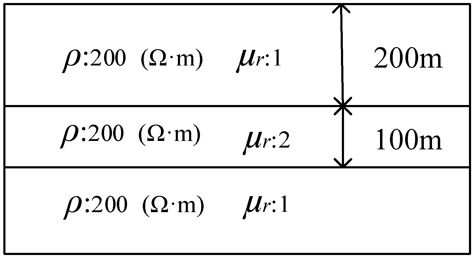
3.1.1. One-Dimensional Magnetic Model

Figure 2 illustrates the presence of a magnetic layer embedded within a conductive half-space with a resistivity of 200 $\mathsf{\Omega }\cdot \mathrm{m}$, while the relative permeability of the magnetic layer is 2. The first layer has a thickness of 200 m, whereas the magnetic layer has a thickness of 100 m. Comparisons of the apparent resistivities at three different frequencies are displayed in

Table 1. $\mathbf{A}-\varphi$ results (3D) and analytical solutions (1D): the apparent resistivities.

Frequencies (Hz)	$\mathit{\rho }$$(\mathsf{\Omega }\cdot \mathbf{m}$)		Realtive Errors (%)
	1D	3D
100	240.3	240.8	0.21
40	231.7	231.4	0.13
20	224.1	223.5	0.27

. It can be observed that the results obtained through the $\mathbf{A}-\varphi$ method exhibit excellent agreement with the analytical solutions [24], as indicated by relative errors below 0.3%.

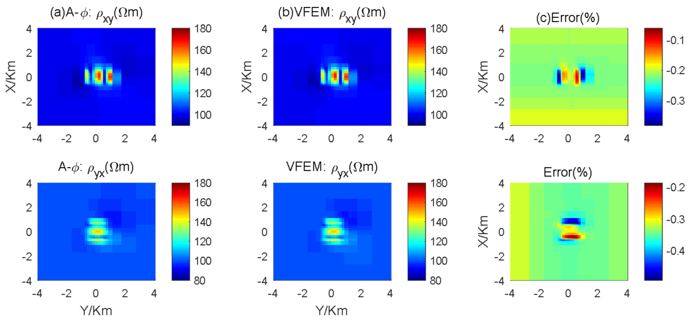
3.1.2. Three-Dimensional Anisotropic Model

To further validate the accuracy of this algorithm, we compared its results with those obtained using the edge-based FEM [20] for a 3D conductive generalized anisotropic and magnetic model. As depicted in Figure 3, an anomaly is embedded within an isotropic half-space of 100 $\mathsf{\Omega }\cdot \mathrm{m}$. The dimensions of the anomaly are 1200 m × 1200 m × 1000 m along the x-, y-, and z-directions, respectively, with a top depth of 250 m. The principal resistivities (${\rho }_x$, ${\rho }_y$, and ${\rho }_z$) of this anomaly are 200 $\mathsf{\Omega }\cdot \mathrm{m}$, 50 $\mathsf{\Omega }\cdot \mathrm{m},$ and 100 $\mathsf{\Omega }\cdot \mathrm{m}$, respectively, while Euler’s angles (${\alpha }_S$, ${\alpha }_D$ and ${\alpha }_L$) are determined using values of 10°, 30°, and 20°, respectively. The relative permeability of this anomaly is 1.5. The frequency used for computation is set at 10 Hz.

Figure 4 displays the apparent resistivities of the xy-mode and yx-mode. The first and second columns correspond to the apparent resistivities obtained from the $\mathbf{A}-\varphi$ method and the edge-based FEM, respectively. The third column shows the relative error, while the upper and lower rows represent xy-mode and yx-mode, respectively. Both methods exhibit a high level of accuracy, with relative errors less than 3%. Our aim is solely to validate this approach; therefore, we refrain from further analysis of Figure 5.

3.2. Typical Models

In this section, we designed a deep-depth model, as well as a marine model. The deep-depth model represents a large-scale magma channel, to some extent, while the marine model approximates marine magnetite deposits.

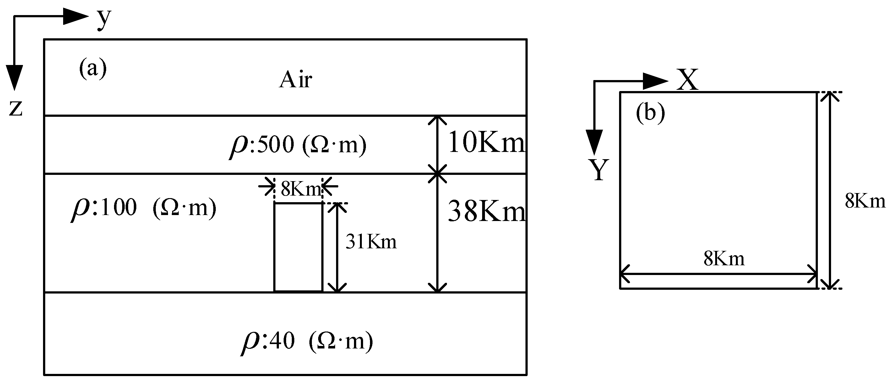
3.2.1. Deep-Depth Model

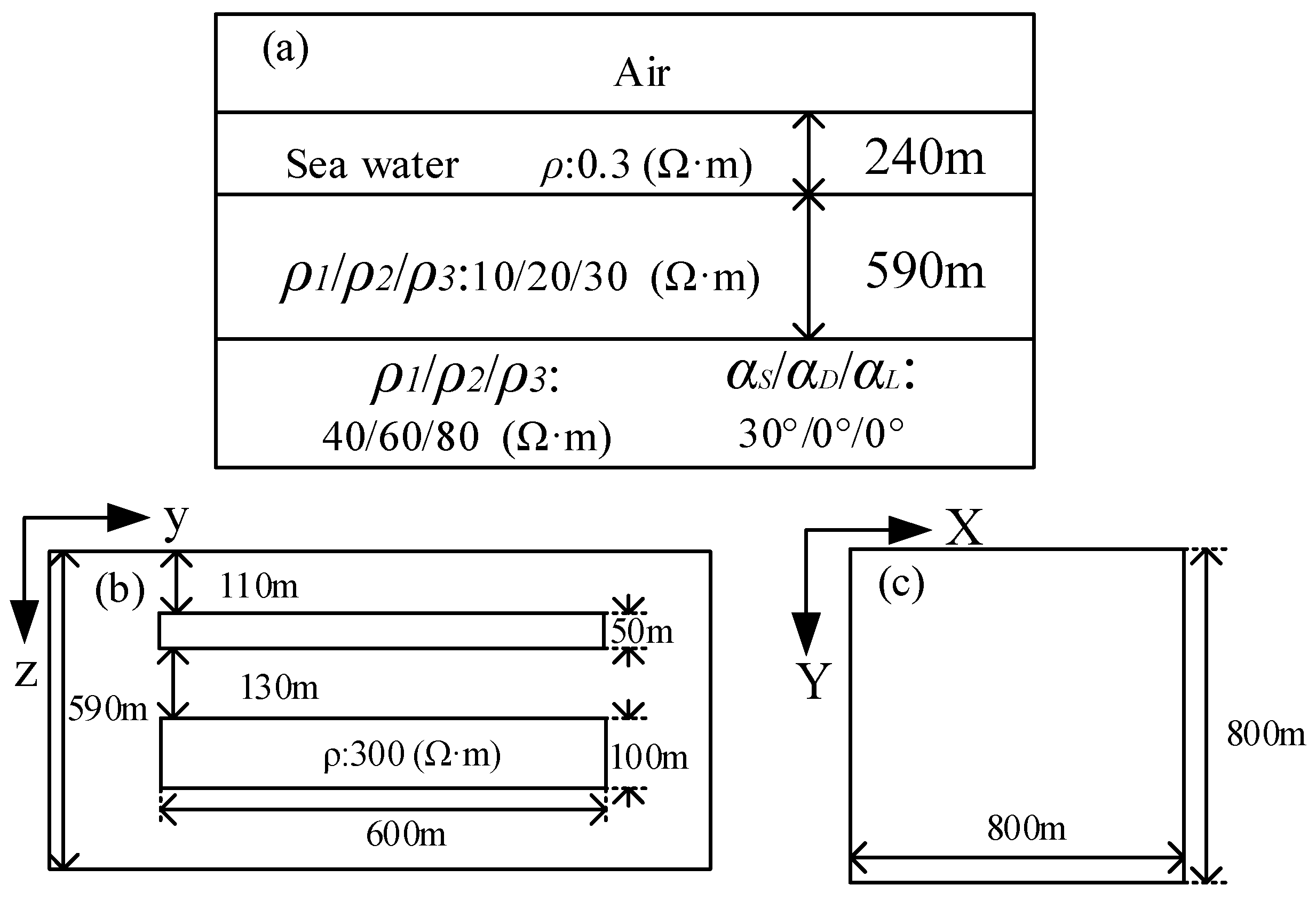
As depicted in Figure 6, the media consists of three layers, with the second layer containing a 3D anomaly. The resistivities of the three layers are 500 $\mathsf{\Omega }\cdot \mathrm{m}$, 100 $\mathsf{\Omega }\cdot \mathrm{m}$, and 40 $\mathsf{\Omega }\cdot \mathrm{m}$, respectively. The first layer has a thickness of 10 km, while the second layer has a thickness of 38 km. The dimensions of the 3D anomaly are 8 km × 8 km × 31 km (in the x-, y-, and z-directions, respectively) with a top depth of 18 km. Four models are generated by varying the resistivities within the embedded anomaly region. The Anis1 model represents an axial conductive anisotropic model with three principal resistivities set at 50 $\mathsf{\Omega }\cdot \mathrm{m}$, 200 $\mathsf{\Omega }\cdot \mathrm{m}$, and 400 $\mathsf{\Omega }\cdot \mathrm{m},$ respectively; the Anis2 model also exhibits axial conductive anisotropy but with three principal resistivity values adjusted to 50 $\mathsf{\Omega }\cdot \mathrm{m}$, 200 $\mathsf{\Omega }\cdot \mathrm{m}$, and 40 $\mathsf{\Omega }\cdot \mathrm{m}$. The Iso1 model corresponds to a conductive isotropic model, with the resistivity value set at 50 $\mathsf{\Omega }\cdot \mathrm{m}$, while the Iso2 model represents another conductive isotropic model, with the resistivity value adjusted to 200 $\mathsf{\Omega }\cdot \mathrm{m}$. The frequency used for computation is 0.001 Hz.

For the four models, Figure 7 and Figure 8 depict the real and imaginary components of the horizontal electric fields induced by two sources, i.e., Source A (Ex = 0, Ey = 1, Ez = 0) and Source B (Ex = 1, Ey = 0, Ez = 0) on the ground surface. The first to fourth columns correspond to the Anis1 model, the Iso1 model, the Iso2 model, and the Anis2 model, respectively. In Figure 7, the first to fourth rows correspond to the real parts of Ex induced by Source A (RExA), Ey induced by Source A (REyA), Ex induced by Source B (RExB), and Ey induced by Source B (REyB), respectively. In Figure 8, the first to fourth rows correspond to the imaginary parts of Ex induced by Source A (IExA), Ey induced by Source A (IEyA), Ex induced by Source B (IExB), and Ey induced by Source B (IEyB), respectively.

3.2.2. Marine Model

The marine model is depicted in Figure 9, where the first layer represents seawater, with a resistivity of 0.3 $\mathsf{\Omega }\cdot \mathrm{m}$ and a thickness of 240 m. The second layer has a thickness of 590 m, exhibits axial conductive anisotropy, and is characterized by three principal resistivities: 10 $\mathsf{\Omega }\cdot \mathrm{m}$, 20 $\mathsf{\Omega }\cdot \mathrm{m}$, and 30 $\mathsf{\Omega }\cdot \mathrm{m},$ respectively. The third layer is also anisotropic conductive, with three principal resistivities: 40 $\mathsf{\Omega }\cdot \mathrm{m}$, 60 $\mathsf{\Omega }\cdot \mathrm{m}$, and 80 $\mathsf{\Omega }\cdot \mathrm{m},$ respectively; additionally, it possesses Euler’s angles of 30°, 0°, and 0°, respectively.

The second layer contains two 3D anomalies: a higher resistive anomaly with a resistivity of 300 $\mathsf{\Omega }\cdot \mathrm{m}$, measuring 800 m × 800 m × 50 m in the x-, y-, and z-directions, respectively, and an upper magnetic anomaly, measuring 800 m × 800 m × 100 m in the x-, y-, and z-directions, respectively. The upper anomaly is characterized by varying relative permeabilities, and its resulting apparent resistivities are presented in Figure 10, while the corresponding phases at the seafloor are shown in Figure 11. These calculations were performed at a frequency of 1 Hz.

In Figure 10, the first to fourth rows correspond to the xx-, xy-, yx-, and yy-mode apparent resistivities, respectively. Meanwhile, the first to fourth columns represent the relative permeabilities of 1, 1.5, 2, and 3, respectively. In Figure 11, the first to fourth rows correspond to the xx-, xy-, yx-, and yy-mode phases, respectively. The first to fourth columns correspond to the relative permeabilities of 1, 1.5, 2, and 3, respectively.

4. Discussion

4.1. Advantages of Mixed Elements over Nodal Elements

For a given mixed nodal and edge-based element, the distribution of $\mathbf{A}$ and $\varphi$ is shown in Figure 1, namely one $\varphi$ on each node and one $\mathbf{A}$ on each edge. In contrast, for a given nodal element, as shown in Figure 12, there are three components of $\mathbf{A}$ ($Ax$,$Ay$,$Az$) and one $\varphi$ at each node. It is evident that the degrees of freedom (DoF) for one nodal element is 32, while it is only 20 for one mixed nodal and edge-based cell.

As shown in

Table 2. Comparison of the stiffness matrix of the two methods.

Method	Grids in x-, y-, and z- Direction	Degrees of Freedom	Number of Non-Zero Elements
Nodal method	20 × 20 × 20	37,044	1,914,046
	35 × 35 × 35	186,624	9,506,418
	50 × 50 × 50	530,604	27,283,608
Mixed nodal and edge-based element method	20 × 20 × 20	35,721	1,290,361
	35 × 35 × 35	182,736	6,817,756
	50 × 50 × 50	522,801	19,763,401

, we compared the DoF and the number of non-zero elements for the two methods with three different grid sizes. The data indicate that the mixed nodal and edge-based element method offers significant advantages, which will become even greater as the grid size increases. For 50 × 50 × 50 grids in the x-, y-, and z-directions, the number of non-zero elements in the mixed element method is only 72.44% that of the nodal element method.

4.2. Typical Models

4.2.1. Deep-Depth Model

The resistivity in the x-direction of the Anis1 model, the Anis2 model, and the Iso1 model is consistently 50 $\mathsf{\Omega }\cdot \mathrm{m}$, while the resistivity in the y-direction of the Anis1 model, the Anis2 model, and the Iso2 model is consistently 200 $\mathsf{\Omega }\cdot \mathrm{m}$.

As depicted in Figure 6, RExB and REyB for the Iso1 model exhibit remarkable similarities to those of the Anis1 model; similarly, RExA and REyA for the Iso2 model closely resemble those of the Anis1 model. Notably, the fourth row mirrors the characteristics observed in the first row. As depicted in Figure 7, IExB and IEyB for the Iso1 model closely resemble those for the Anis1 model; IExA and IEyA for the Iso2 model demonstrate a similar pattern to those for the Anis1 model. Again, the fourth row closely resembles the first row.

Comparing the electric fields of the Anis1 model with those of the Iso1 model, it can be inferred that if a principal resistivity is oriented in the x-direction, then the horizontal electric fields induced by Ex are primarily influenced by this principal resistivity. Similarly, comparing the Anis1 model with the Iso2 model leads to the conclusion that when a principal resistivity is oriented in the y-direction, the horizontal electric fields induced by Ey are predominantly affected by this principal resistivity. Lastly, comparing the Anis1 model with the Anis2 model reveals that if a principal resistivity is oriented in the z-direction, it has minimal impact on the horizontal electric fields. This third finding is consistent with the previous two.

Considering the relationship between magnetic fields and electric fields, we can also infer that: (1) if a principal resistivity is oriented in the x-direction, then the horizontal magnetic fields induced by Ex are primarily influenced by this principal resistivity; (2) if a principal resistivity is oriented in the y-direction, then the horizontal magnetic fields induced by Ey are predominantly affected by this principal resistivity; (3) if a principal resistivity is oriented in the z-direction, it has minimal impact on the horizontal magnetic fields.

Considering the relationship between electromagnetic fields and apparent resistivities or phases, we can further infer that: (1) if a principal resistivity is oriented in the x-direction, then the xy-mode apparent resistivity and the xy-mode phase are mainly influenced by this principal resistivity; (2) if a principal resistivity is oriented in the y-direction, then the yx-mode apparent resistivity and the yx-mode phase are mainly influenced by this principal resistivity; (3) if a principal resistivity is oriented in the z-direction, then this principal resistivity exhibits almost no influence on the MT responses. These phenomena are also consistent with the conclusions put forth in Reference [20].

4.2.2. Marine Model

The data in Figure 9 demonstrate that the apparent resistivities of the xx-, xy-, yx-, and yy-modes increase as the relative permeability increases, with the first to fourth rows corresponding to these modes, respectively. These findings highlight the significant influence of high relative permeability on apparent resistivities. The results in Figure 10 show that the relative permeability also has a significant effect on the phases.

In this case, there are two 3D anomalies, i.e., a higher resistivity anomaly and a magnetic anomaly. Specifically, the higher resistive anomaly’s MT responses are greatly affected by the magnetic anomaly. This suggests that the apparent resistivities of the lower resistivity anomaly may manifest as higher apparent resistivities due to the presence of the magnetic anomaly. These findings are also consistent with those observed in the previous study by Xiao et al. [20].

5. Conclusions

A 3D numerical modeling algorithm is presented that utilizes mixed nodal and edge-based elements with Coulomb-gauged EM potentials in conductive anisotropic and magnetic media. This algorithm effectively reduces the number of unknowns compared to that of the nodal element method. The accuracy of this algorithm is validated by comparing its results with analytical solutions for a two-layer magnetic medium and is further confirmed through comparisons with results obtained from the edge-based FEM for a 3D conductive generalized anisotropic and magnetic model. Subsequently, several typical models are studied in detail. It can be concluded that:

(1)

The algorithm, whether applied at low frequencies (0.001 Hz) or in cases of high resistive contrasts, demonstrates robust performance; it works well for modeling deep Earth and ocean models with strong resistivity contrasts.

(2)

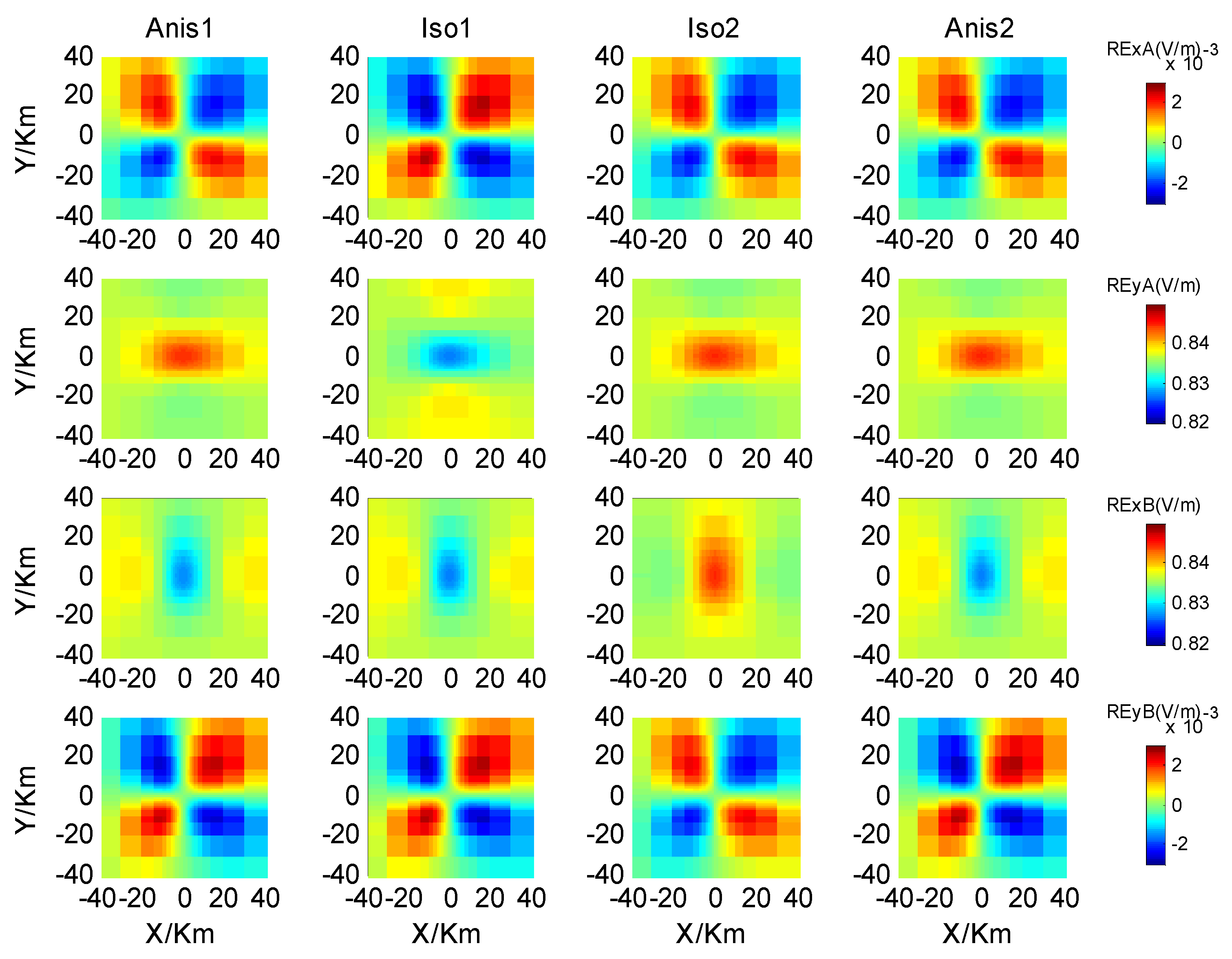
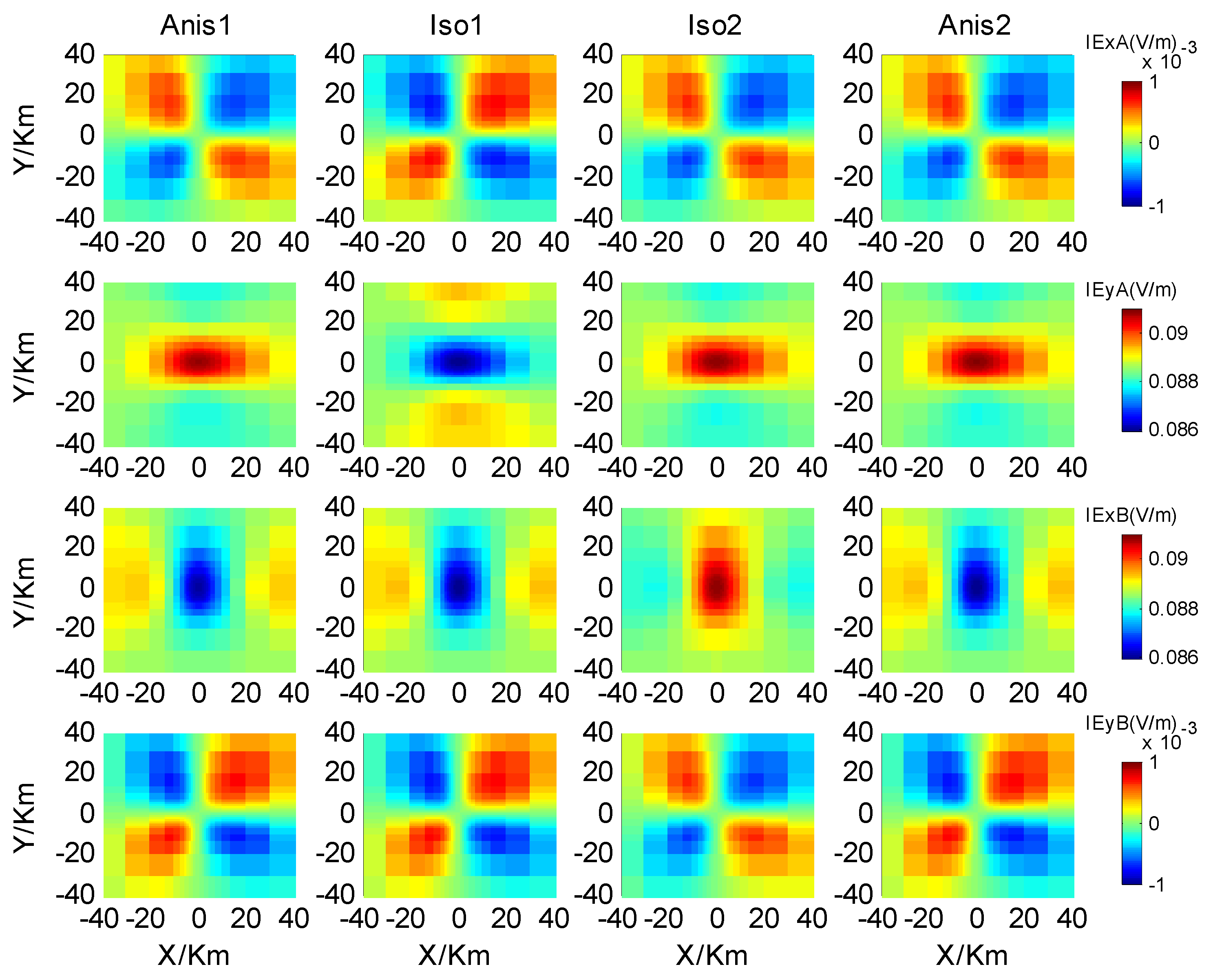
The horizontal electric fields induced by Ex are predominantly influenced by conductivity in the x-direction, while the horizontal electric fields induced by Ey are primarily influenced by conductivity in the y-direction. Conductivity in the z-direction has a negligible impact on the horizontal electric fields. Additionally, it would be helpful to explain the effect of anisotropy on MT responses in practical surveys.

(3)

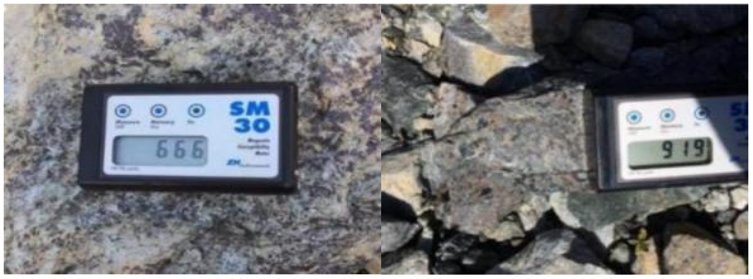
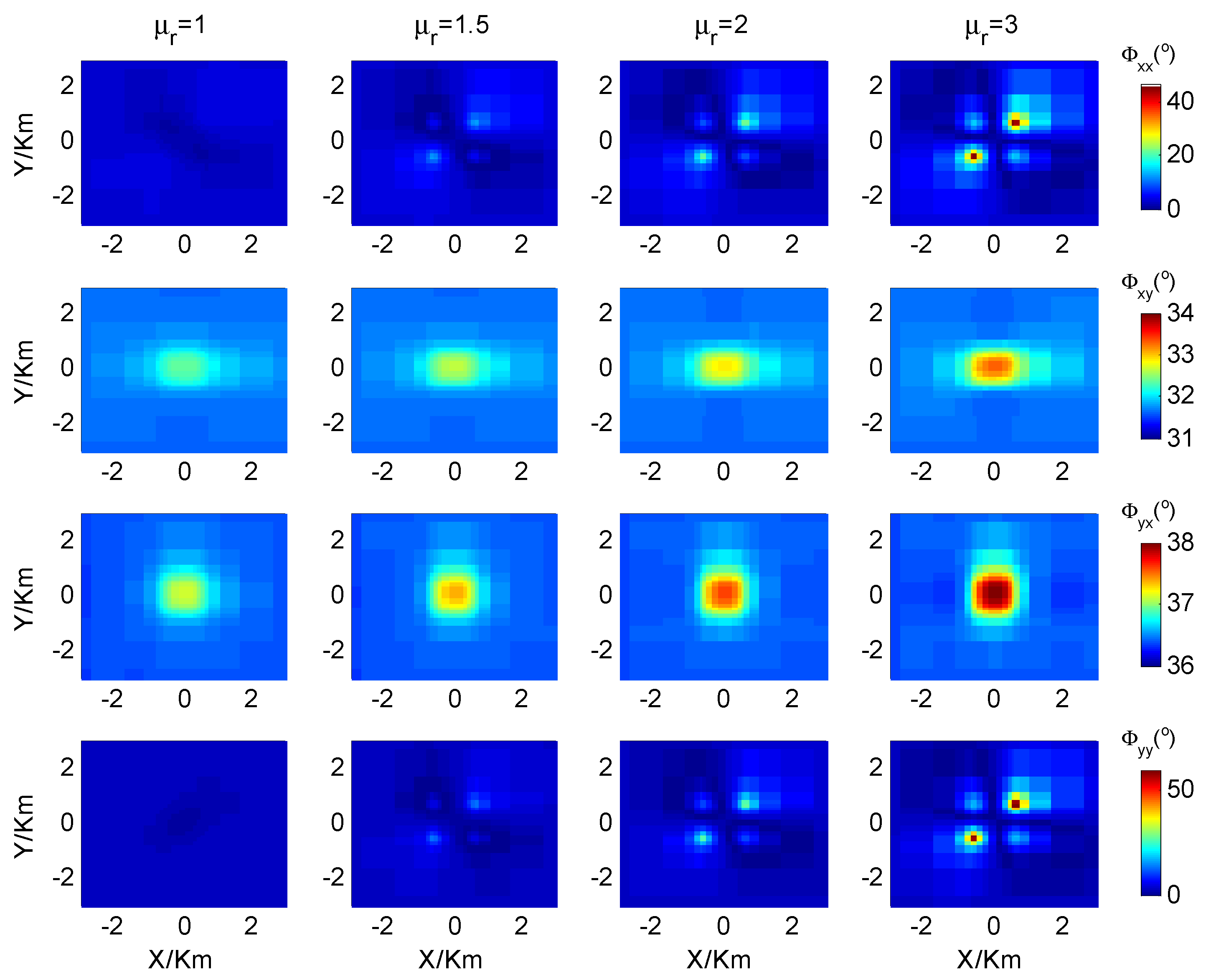
More attention on evaluating the influences of magnetic permeability in magnetite-rich areas is needed. The practical geological environment of Earth is extremely complex; the apparent resistivities and phases could be significantly distorted, or even reversed, due to the existence of non-zero magnetic susceptibility.

Furthermore, this algorithm also provides a robust future forward modeling method for practical 3D MT inversion in conductive anisotropic and magnetic media.

References

1. Chave, A.D.; Jones, A.G. (Eds.) The Magnetotelluric Method: Theory and Practice; Cambridge University Press: Cambridge, UK, 2012. [Google Scholar]
2. Varentsov, I.M.; Kulikov, V.A.; Yakovlev, A.G.; Yakovlev, D.V. Possibilities of magnetotelluric methods in geophysical exploration for ore minerals. Izv. Phys. Solid Earth 2013, 49, 309–328. [Google Scholar] [CrossRef]
3. Tan, H.D.; Yu, Q.F.; Booker, J.; Wei, W. Magnetotelluric three-dimensional modeling using the staggered-grid finite difference method. Chin. J. Geophys. 2003, 46, 705–711. [Google Scholar]
4. Cai, H.; Xiong, B.; Han, M.; Zhdanov, M. 3D controlled-source electromagnetic modeling in anisotropic medium using edge-based finite element method. Comput. Geosci. 2014, 73, 164–176. [Google Scholar] [CrossRef]
5. Ren, Z.H.; Chen, C.; Tang, J. Accurate volume integral solutions of direct current resistivity potentials for inhomogeneous conductivities in half space. J. Appl. Geophys. 2018, 151, 40–46. [Google Scholar] [CrossRef]
6. Haber, E.; Ascher, U.M.; Aruliah, D.A.; Oldenburg, D.W. Fast simulation of 3D electromagnetic problems using potentials. J. Comput. Phys. 2000, 163, 150–171. [Google Scholar] [CrossRef]
7. Badea, E.A.; Everett, M.E.; Newman, G.A.; Biro, O. Finite-element analysis of controlled-source electromagnetic induction using Coulomb-gauged potentials. Geophysics 2001, 66, 786–799. [Google Scholar] [CrossRef]
8. Xiao, T.; Huang, X.; Wang, Y. Three-dimensional magnetotelluric modelling in anisotropic media using the A-phi method. Explor. Geophys. 2019, 50, 31–41. [Google Scholar] [CrossRef]
9. Yu, N.; Chen, Z.; Wu, X.; Kong, W.; Chen, H.; Li, T.; Feng, X. Unstructured grid finite element modeling of the three-dimensional magnetotelluric responses in a model with arbitrary conductivity and magnetic susceptibility anisotropies. IEEE Trans. Geosci. Remote Sens. 2024, 62, 2002013. [Google Scholar] [CrossRef]
10. Linde, N.; Pedersen, L.B. Evidence of electrical anisotropy in limestone formations using the RMT technique. Geophysics 2004, 69, 909–916. [Google Scholar] [CrossRef]
11. Wannamaker, P.E. Anisotropy versus heterogeneity in continental solid earth electromagnetic studies: Fundamental response characteristics and implications for physicochemical state. Surv. Geophys. 2005, 26, 733–765. [Google Scholar] [CrossRef]
12. Evans, R.L.; Hirth, G.; Baba, K.; Forsyth, D.; Chave, A.; Mackie, R. Geophysical evidence from the MELT area for compositional controls on oceanic plates. Nature 2005, 437, 249. [Google Scholar] [CrossRef] [PubMed]
13. Pek, J.; Verner, T. Finite-difference modelling of magnetotelluric fields in two-dimensional anisotropic media. Geophys. J. Int. 1997, 128, 505–521. [Google Scholar] [CrossRef]
14. Kong, W.; Lin, C.; Tan, H.; Peng, M.; Tong, T.; Wang, M. The effects of 3D electrical anisotropy on magnetotelluric responses: Synthetic case studies. J. Environ. Eng. Geophys. 2018, 23, 61–75. [Google Scholar] [CrossRef]
15. Li, Y. Finite Element Modeling of Electromagnetic Fields in Two-and Three-Dimensional Anisotropic Conductivity Structures. Ph.D. Thesis, University of Gottingen, Gottingen, Germany, 2000. [Google Scholar]
16. Löwer, A.; Junge, A. Magnetotelluric Transfer Functions: Phase Tensor and Tipper Vector above a Simple Anisotropic Three-Dimensional Conductivity Anomaly and Implications for 3D Isotropic Inversion. Pure Appl. Geophys. 2017, 174, 2089–2101. [Google Scholar] [CrossRef]
17. Xiao, T.; Liu, Y.; Wang, Y.; Fu, L.Y. Three-dimensional magnetotelluric modeling in anisotropic media using edge-based finite element method. J. Appl. Geophys. 2018, 149, 1–9. [Google Scholar] [CrossRef]
18. Liu, Y.; Xu, Z.; Li, Y. Adaptive finite element modelling of three-dimensional magnetotelluric fields in general anisotropic media. J. Appl. Geophys. 2018, 151, 113–124. [Google Scholar] [CrossRef]
19. Zhou, J.; Hu, X.; Xiao, T.; Cai, H.; Li, J.; Peng, R.; Long, Z. Three-dimensional edge-based finite element modeling of magnetotelluric data in anisotropic media with a divergence correction. J. Appl. Geophys. 2021, 189, 104324. [Google Scholar] [CrossRef]
20. Xiao, T.; Wang, Y.; Huang, X.; He, G.; Liu, J. Magnetotelluric responses of three-dimensional conductive and magnetic anisotropic anomalies. Geophys. Prospect. 2020, 68, 1016–1040. [Google Scholar] [CrossRef]
21. Jin, J.M. The Finite Element Method in Electromagnetics, 2nd ed.; John Wiley and Sons: New York, NY, USA, 2002. [Google Scholar]
22. Mickus, K. Magnetic Method. 2023. Available online: https://www.researchgate.net/publication/228994566_Magnetic_Method (accessed on 21 July 2024).
23. Chen, L.; Xiao, T.; Liu, J.; Zheng, X.; Liu, J.; Wang, Y. One-dimensional magnetotelluric modeling in magnetic and resistive axial anisotropic media. Prog. Geophys. 2022, 37, 2373–2380. (In Chinese) [Google Scholar]
24. Yadav, G.S.; Lal, T. A Fortran 77 program for computing magnetotelluric response over a stratified earth with changing magnetic permeability. Comput. Geosci. 1997, 23, 1035–1038. [Google Scholar] [CrossRef]
Figure 1. Mixed nodal and edge-based elements, along with their respective local coordinate systems.
Applsci 14 09019 g001
Figure 2. Magnetic susceptibility of magnetite in Huayang, Shaanxi Province, China (666/919 × 10−3 SI).
Applsci 14 09019 g002
Figure 3. One-dimensional magnetic model.
Applsci 14 09019 g003
Figure 4. Three-dimensional anisotropic model: (a) section view; (b) plan view.
Applsci 14 09019 g004
Figure 5. Comparison with the edge-based FE method: (a) the left column corresponds to the A ϕ method; (b) the middle column corresponds to the edge-based FE method (VFEM); (c) the right column corresponds to the relative errors.
Applsci 14 09019 g005
Figure 6. Deep-depth model: (a) the section view; (b) the plan view of the 3D anomaly.
Applsci 14 09019 g006
Figure 7. The real parts of the electric fields at the ground surface for the Anis1 model, the Iso1 model, the Iso2 model, and the Anis2 model.
Applsci 14 09019 g007
Figure 8. The imaginary parts of the electric fields at the ground surface for the Anis1 model, the Iso1 model, the Iso2 model, and the Anis2 model.
Applsci 14 09019 g008
Figure 9. Marine model: (a) the cross-sectional view of the entire model; (b) the cross-sectional view of the second layer containing two 3D anomalies; (c) the top-down view of the 3D anomalies.
Applsci 14 09019 g009
Figure 10. The apparent resistivities on the seafloor for the upper anomaly, with varying relative permeabilities.
Applsci 14 09019 g010
Figure 11. The phases on the seafloor for the upper anomaly, with varying relative permeabilities.
Applsci 14 09019 g011
Figure 12. The distribution of A and ϕ on a nodal element.
Applsci 14 09019 g012