Stability Comparison of Grid-Connected Inverters Considering Voltage Feedforward Control in Different Domains

Abstract

Under the background of high permeability, voltage feedforward control may further weaken the stability of grid-connected inverter (GCI) systems and may cause sub-synchronous oscillation in extreme cases. To solve this problem, this paper firstly considers the influence of the frequency coupling effect and voltage feedforward control, and adopts the harmonic linearization method to construct the L-type GCI sequence admittance model with PI (proportional integral) control and PR (proportional resonant) control, respectively. By comparing the sequence admittance characteristics of the GCI under two control strategies, combined with the sequence admittance model and Nyquist criterion, this paper analyzes the influence of voltage feedforward and control parameters on the stability of the GCI under two control strategies. The results show that the stability of GCI under PR control is slightly better than that under PI control. At the same time, the voltage feedforward control does reduce the stability of the GCI system under the two control strategies. Finally, the accuracy of the theoretical analysis is verified by simulation and experiment.

1. Introduction

With the widespread application of renewable energies such as photovoltaic and wind in power systems, the power electronic characteristics of these systems are becoming increasingly evident. As the key equipment for new energy integration, inverters have garnered considerable attention [1,2]. However, there is a risk of oscillation in the interaction between the GCI and the power grid. Particularly when connected to a weak grid, this situation increases the likelihood of inducing broadband oscillations, which pose a serious threat to the stable operation of the power system [3,4,5]. Therefore, an in-depth analysis of the stability of GCIs holds important practical significance.

Recently, the impedance analysis method has garnered significant attention in the study of inverter grid-connected stability due to its clear physical principles, straightforward measurability, and verifiability [6,7,8]. Currently, many studies have established impedance models of GCI that consider the current loop, PLL (phase-locked loop), and delay [9,10]. However, the literature [11] points out that ignoring the frequency coupling characteristics can make the established impedance model inaccurate, which may lead to errors in stability analysis. In view of this, reference [12] has established a sequence impedance model considering the frequency coupling effect and has analyzed the mechanism of this effect. In references [13,14], a frequency coupling admittance model of an L-type GCI considering various factors such as PLL, voltage outer loop, and current inner loop is established, and the GNC (generalized Nyquist criterion) is utilized to assess the stability of the system. Therefore, the use of impedance analysis for stability analysis has been widely studied.

Based on the control domain differences, control methods can be categorized into PR control in the time domain and PI control in the dq (direct-quadrature) domain. It has been established that, in terms of steady-state performance, time-domain PR control and dq-domain PI control are equivalent [15]. However, under conditions of a weak power grid, the stability of the two current-controlled GCI systems may differ [16]. Currently, the stability analysis of GCI systems controlled by PI in the dq domain using impedance analysis has been extensively studied [17,18,19,20]. However, research on the stability analysis of GCI systems based on time-domain PR control using impedance analysis is limited. Moreover, the impact of voltage feedforward control on stability has not been considered in the aforementioned literature.

Voltage feedforward control is commonly used to enhance the dynamic performance of GCI systems, suppress background harmonics, and alleviate imbalances caused by grid voltage fluctuations [21,22,23,24]. However, in practical applications, it has been observed that voltage feedforward control significantly impacts the impedance characteristics and stability of the GCI system [25]. Therefore, it is crucial to analyze the impedance characteristics and stability of the GCI system with voltage feedforward control implemented.

To address the stability analysis of the GCI system with different domain controls and considering voltage feedforward, a frequency coupling admittance model under time-domain PR control and dq-domain PI control is established using the multi-harmonic linearization method. The stability of these controls is then compared. This analysis elucidates the significance of different domain controls and voltage feedforward control in enhancing the stability of the GCI system.

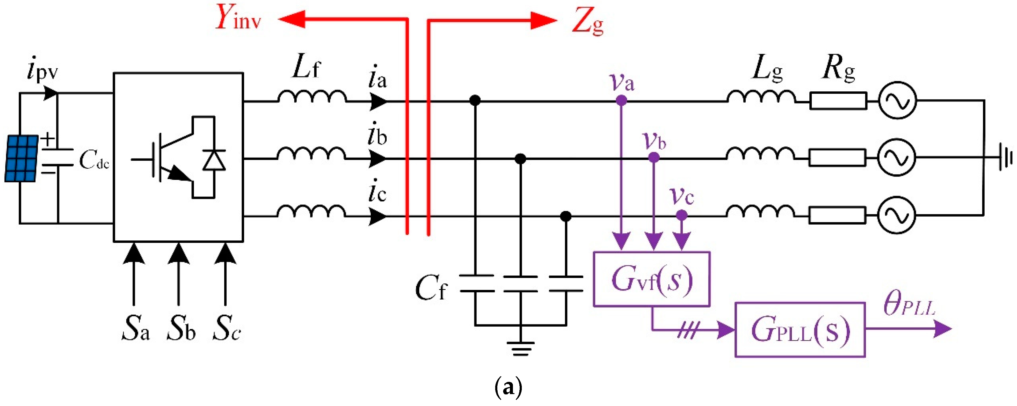
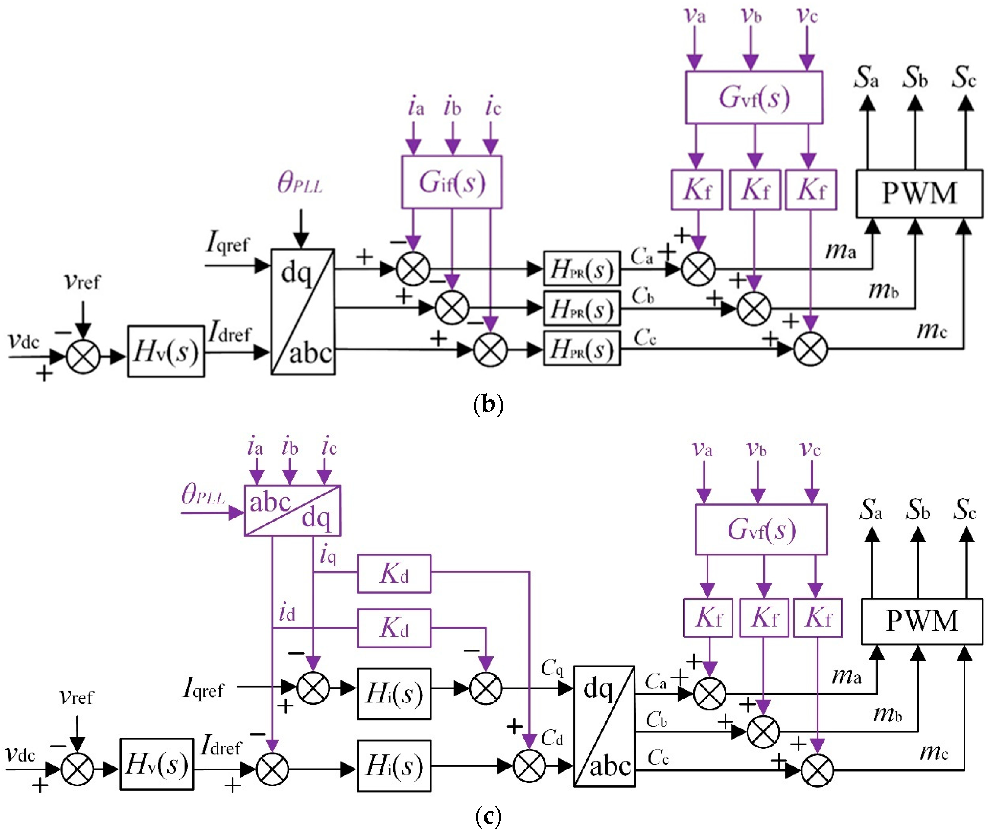
2. GCI System Structure with Different Domain Controls

Figure 1 illustrates the circuit topology and control structure of the three-phase GCI system. In Figure 1, L_f represents the filter inductor, and C_f denotes the filter capacitor; v_a, v_b, and v_c are the three-phase voltages at the grid connection point; i_a, i_b, and i_c are the currents through the filter inductor; R_g and L_g represent the equivalent resistance and inductance of the grid, respectively; C_dc is the equivalent capacitance; i_pv is the photovoltaic output current; v_ref is the reference value for the DC bus voltage; I_dref and I_qref are the reference values for the dq-domain grid-connected currents, respectively; H_v(s) is the voltage-loop PI controller function; K_d represents the decoupling coefficient; K_f denotes the voltage feedforward coefficient; m_a, m_b, and m_c are the three-phase modulation signals; S_a, S_b, and S_c are the three-phase switching signals.

The expressions of the PR and PI controllers used in the current inner loop are as follows:

$$\left\{\begin{array}{l}{H}_{\mathrm{PR}}(s)=K_{\mathrm{p}1}+{\displaystyle \frac{2K_{r}s}{s^2+{\omega }_1^2}}\\ H_{\mathrm{PI}}(s)=K_{\mathrm{p}2}+{\displaystyle \frac{K_i}{s}}\end{array}\right.$$

(1)

In the formula, ω₁ is the fundamental angular frequency, K_p1 and K_r are the proportional coefficient and resonance coefficient of the PR controller, respectively, and K_p2 and K_i are the proportional coefficient and resonance coefficient of the PI controller, respectively.

According to the literature [26], there is an equivalent relationship between the PR controller adopted in the phase domain and the PI controller in the dq domain, that is,

$$H_{\mathrm{PR}}(s)={\displaystyle \frac{1}{2}}[H_{\mathrm{PI}}(s+j{\omega }_1)+H_{\mathrm{PI}}(s-j{\omega }_1)]$$

(2)

Therefore, this paper analyzes the parameter alignment between the PR and PI controllers as follows: K_p1 = K_p2, K_r = K_i/2.

3. Sequence Admittance Modeling of Grid-Connected Inverter

The frequency coupling effect significantly influences the admittance characteristic frequency of the GCI. Therefore, considering factors such as frequency coupling, control delay, and voltage feedforward link, the sequence admittance model of the GCI under different domain controls is derived.

The filters of voltage and current sampling are described as follows:

$$\left\{\begin{array}{l}{G}_{\mathrm{vf}}(s)={\displaystyle \frac{1}{(1+s/{\omega }_{\mathrm{v}})}}\\ G_{\mathrm{if}}(s)={\displaystyle \frac{1}{(1+s/{\omega }_{\mathrm{i}})}}\end{array}\right.$$

(3)

In the formula, ω_v and ω_i represent the angular frequencies of the voltage and current sampling filters, respectively. For simplified expressions, s = ±j2πf_p, s₁ = ±j2πf₁, s_p1 = ±j2π(f_p-2f₁), and s₂ = ±j2π(f_p-f₁) are defined.

From the system main circuit topology diagram shown in Figure 1a, there is a relationship between the inverter bridge arm voltage, output voltage, and output current:

$$L_f{\displaystyle \frac{d}{dt}}\left[\begin{array}{c}{i}_a\\ i_b\\ i_c\end{array}\right]=\left[\begin{array}{c}{e}_a\\ e_b\\ e_c\end{array}\right]-\left[\begin{array}{c}{v}_a\\ v_b\\ v_c\end{array}\right]$$

(4)

According to the frequency coupling effect, when a positive sequence voltage disturbance at frequency f_p is introduced at the grid connection point, it induces a positive sequence response current at the same frequency f_p and a negative sequence response current at frequency f_p-2f₁. As the negative sequence response current moves through the grid impedance, it induces a matching negative sequence voltage disturbance at the same frequency. Consequently, the time-domain expressions for the voltage and current of phase A at the grid connection point are described as follows:

$$\begin{array}{cc}\hfill v_a(t)=& V_1\cos ({\omega }_{1}t)+V_{\mathrm{p}}\cos ({\omega }_{p}t+{\phi }_{\mathrm{vp}})\hfill \\ & +V_{\mathrm{p}2}\cos ({\omega }_{\mathrm{p}2}t+{\phi }_{\mathrm{vp}2})\hfill \end{array}$$

(5)

$$\begin{array}{cc}\hfill i_a(t)=& I_1\cos ({\omega }_{1}t+{\phi }_{\mathrm{i}1})+I_p\cos ({\omega }_{\mathrm{p}}t+{\phi }_{\mathrm{ip}})\hfill \\ & +I_{\mathrm{p}2}\cos ({\omega }_{\mathrm{p}2}t+{\phi }_{\mathrm{ip}2})\hfill \end{array}$$

(6)

In the formula, the voltage amplitudes V₁, V_p, and V_p2 represent the fundamental, positive sequence disturbance, and negative sequence coupling frequencies, respectively. The angular frequencies ω₁, ω_p, and ω_p2 similarly represent the fundamental, positive sequence disturbance, and negative sequence coupling frequencies. Additionally, the initial phase angles for the disturbance voltages φ_vp and φ_vp2 are specified at the positive and negative sequence disturbance frequencies. The currents I₁, I_p, and I_p2 for these frequencies are matched with their respective initial phase angles φ_i1, φ_ip, and φ_ip2, highlighting the coherent response of the system across these varied conditions.

According to Formulas (5) and (6), the frequency domain expression can be expressed as follows:

$$V_a=\left\{\begin{array}{l}{\mathbf{V}}_1,f=\pm f_1\\ {\mathbf{V}}_{\mathrm{p}},f=\pm f_p\\ {\mathbf{V}}_{\mathrm{p}2},f=\pm (f_p-2f_1)\end{array}\right.,i_a=\left\{\begin{array}{l}{\mathbf{I}}_1,f=\pm f_1\\ {\mathbf{I}}_{\mathrm{p}},f=\pm f_p\\ {\mathbf{I}}_{\mathrm{p}2},f=\pm (f_p-2f_1)\end{array}\right.$$

(7)

In the formulas, V₁ = V₁/2, V_p = (V_p/2)e^±jφvp, V_p2 = (V_p2/2)e^±jφvp2, I₁ = (I₁/2)e^±jφi1, I_p = (I_p/2)e^±jφip, and I_p2 = (I_p2/2)e^±jφip2.

3.1. Phase-Locked Loop Modeling

To ensure the rationality of the method in this paper, the synchronous reference frame PLL is used in the control strategies depicted in Figure 1. Consequently, the transfer function of the PLL is as follows:

$$H_{\mathrm{PLL}}(s)=G_{\mathrm{PI}\text{\_}\mathrm{PLL}}(s)/s$$

(8)

In the formula, G_{PI_PLL} = K_{P_PLL} + K_{i_PLL}/s.

Taking into account the frequency coupling effect, θ_PLL(t) = Δθ_PLL(t) + θ₁(t) is established. Consequently, the frequency domain representation of θ_PLL(t) at the frequency f = ± (f_p − f₁) is articulated as follows:

$$\Delta {\theta }_{\mathrm{PLL}}[f]=T_{\mathrm{PLL}}(s_2)G_{\mathrm{vf}}(s){\mathbf{V}}_{\mathrm{p}}+T_{\mathrm{PLL}1}(s_2)G_{\mathrm{vf}}(s_{\mathrm{p}2}){\mathbf{V}}_{\mathrm{p}2}$$

(9)

In the formula, T_PLL(s₂) = $\mp$jH_PLL(s₂)/(1 + V₁H_PLL(s₂)), T_PLL1(s₂) = ±jH_PLL(s₂)/(1 + V₁H_PLL(s₂)).

3.2. Voltage Outer Loop Modeling

According to the law of conservation of energy, and by ignoring energy losses, it can be inferred that the power on the DC side is equivalent to that on the AC side. Therefore, it follows that

$$\begin{array}{l}{v}_{\mathrm{dc}}(i_{\mathrm{pv}}-s{C}_{\mathrm{dc}}{v}_{\mathrm{dc}})\\ =(v_{\mathrm{a}}+s{L}_{\mathrm{f}}{i}_{\mathrm{a}})i_{\mathrm{a}}+(v_{\mathrm{b}}+s{L}_{\mathrm{f}}{i}_{\mathrm{b}})i_{\mathrm{b}}+(v_{\mathrm{c}}+s{L}_{\mathrm{f}}{i}_{\mathrm{c}})i_{\mathrm{c}}\end{array}$$

(10)

In the formula, v_dc is the DC side voltage.

The frequency domain expression of Formula (10) at frequency f = ±(f_p-f₁) is as follows:

$$v_{\mathrm{dc}}[f]={\displaystyle \frac{3[({\mathbf{V}}_1^{*}+s_2{L}_{\mathrm{f}}{\mathbf{I}}_1^{*}){\mathbf{I}}_{\mathrm{p}}+({\mathbf{V}}_1+s_2{L}_{\mathrm{f}}{\mathbf{I}}_1){\mathbf{I}}_{\mathrm{p}2}+{\mathbf{I}}_1^{*}{\mathbf{V}}_{\mathrm{p}}+{\mathbf{I}}_1{\mathbf{V}}_{\mathrm{p}2}]}{i_{\mathrm{pv}}-s_2{C}_{\mathrm{dc}}{v}_{\mathrm{dc}}}}$$

(11)

In the formula, “*” represents conjugation, and v_dc is the DC side voltage.

By simplifying Formula (11), the expression for v_dc [ f] is articulated as follows:

$$v_{dc}[f]=F_{\mathrm{v}}{\mathbf{V}}_{\mathrm{p}}+F_{\mathrm{v}2}{\mathbf{V}}_{\mathrm{p}2}+F_{\mathrm{i}}{\mathbf{I}}_{\mathrm{p}}+F_{\mathrm{i}2}{\mathbf{I}}_{\mathrm{p}2}$$

(12)

In the formula,

$$\left[\begin{array}{cc}{F}_{\mathrm{v}}& F_{\mathrm{v}2}\\ F_{\mathrm{i}}& F_{\mathrm{i}2}\end{array}\right]=\left[\begin{array}{cc}{\displaystyle \frac{3{\mathbf{I}}_1^{*}}{i_{\mathrm{pv}}-s_2{C}_{\mathrm{dc}}{v}_{\mathrm{dc}}}}& {\displaystyle \frac{3{\mathbf{I}}_1}{i_{\mathrm{pv}}-s_2{C}_{\mathrm{dc}}{v}_{\mathrm{dc}}}}\\ {\displaystyle \frac{3({\mathbf{V}}_1^{*}+s_2{L}_{\mathrm{f}}{\mathbf{I}}_1^{*})}{i_{\mathrm{pv}}-s_2{C}_{\mathrm{dc}}{v}_{\mathrm{dc}}}}& {\displaystyle \frac{3({\mathbf{V}}_1+s_2{L}_{\mathrm{f}}{\mathbf{I}}_1)}{i_{\mathrm{pv}}-s_2{C}_{\mathrm{dc}}{v}_{\mathrm{dc}}}}\end{array}\right]$$

3.3. Sequential Admittance Modeling of GCI by PR

According to the phase-domain PR-controlled GCI shown in Figure 1b, the reference value of the grid-connected current under the dq axis is defined as follows:

$$\left\{\begin{array}{l}{i}_{\mathrm{dref}}=(G_{\mathrm{vf}}(s_2)v_{\mathrm{dc}}-v_{\mathrm{ref}})H_{\mathrm{v}}(s_2)\\ i_{\mathrm{qref}}=0\end{array}\right.$$

(13)

In the formula, H_v(s₂) = K_p + K_i/s is the PI controller used in the voltage outer loop.

As shown in the control structure diagram of the GCI regulated by phase-domain PR in Figure 1b, the reference value for the grid-connected current along the dq axis is subjected to an inverse transformation, and the frequency domain representation for the a-phase grid-connected current is specified as follows:

$$i_{\mathrm{aref}}=i_{\mathrm{dref}}[f]\otimes \cos {\theta }_{\mathrm{PLL}}[f]-i_{\mathrm{qref}}[f]\otimes \sin {\theta }_{\mathrm{PLL}}[f]$$

(14)

In the formula, $⨂$ convolution operation is denoted.

It can be deduced that:

$$I_{aref}[f]=\left\{\begin{array}{l}{\mathbf{I}}_1,f=\pm f_1\\ {\displaystyle \frac{1}{2}}[v_{\mathrm{dc}}[f]G_{\mathrm{vf}}(s_2)H_{\mathrm{v}}(s_2)\\ +j{I}_1(T_{\mathrm{PLL}}(s_2)G_{\mathrm{vf}}(s){\mathbf{V}}_{\mathrm{p}}+T_{\mathrm{PLL}1}(s_2)G_{\mathrm{vf}}(s_{\mathrm{p}2}){\mathbf{V}}_{\mathrm{p}2})],f=\pm f_p\\ {\displaystyle \frac{1}{2}}[v_{dc}[f]G_{\mathrm{vf}}(s_2)H_{\mathrm{v}}(s_2)\\ -j{I}_1(T_{\mathrm{PLL}}(s_2)G_{\mathrm{vf}}(s){\mathbf{V}}_{\mathrm{p}}+T_{\mathrm{PLL}1}(s_2)G_{\mathrm{vf}}(s_{\mathrm{p}2}){\mathbf{V}}_{\mathrm{p}2})],f=\pm (f_p-2f_1)\end{array}\right.$$

(15)

Through the PR controller and the voltage feedforward link, the modulation signal’s expression is delineated as follows:

$$c_a[f]=\left\{\begin{array}{l}{H}_{\mathrm{PR}}(s)(I_{\mathrm{aref}}[f]-G_{\mathrm{if}}(s){\mathbf{I}}_{\mathrm{p}})+K_{\mathrm{f}}{G}_{\mathrm{vf}}(s){\mathbf{V}}_{\mathrm{p}},f=\pm f_p\\ H_{\mathrm{PR}}(s_{\mathrm{p}2})(I_{\mathrm{aref}}[f]-G_{\mathrm{if}}(s_{\mathrm{p}2}){\mathbf{I}}_{\mathrm{p}2})+K_{\mathrm{f}}{G}_{\mathrm{vf}}(s_{\mathrm{p}2}){\mathbf{V}}_{\mathrm{p}2},f=\pm (f_p-2f_1)\end{array}\right.$$

(16)

Based on Figure 1, the subsequent relationships can be derived:

$$s{L}_f{i}_a=K_{\mathrm{pwm}}{v}_{\mathrm{dc}}{G}_{\mathrm{del}}(s)(c_a+K_{\mathrm{f}}{G}_{\mathrm{vf}}(s)v_a)-v_a$$

(17)

In the formula, control delay G_del(s) = e⁻¹.^5TsS.

Combined with the formula, the following can be obtained:

$$\left[\begin{array}{l}{\mathbf{I}}_{\mathrm{p}}\\ {\mathbf{I}}_{\mathrm{p}2}\end{array}\right]=-\left[\begin{array}{cc}{\mathrm{Y}}_{11\text{\_}\mathrm{PR}}& {\mathrm{Y}}_{12\text{\_}\mathrm{PR}}\\ {\mathrm{Y}}_{21\text{\_}\mathrm{PR}}& {\mathrm{Y}}_{22\text{\_}\mathrm{PR}}\end{array}\right]\left[\begin{array}{l}{\mathbf{V}}_{\mathrm{p}}\\ {\mathbf{V}}_{\mathrm{p}2}\end{array}\right]$$

(18)

$$\left[\begin{array}{l}{H}_{\mathrm{p}}\\ H_{\mathrm{p}2}\end{array}\right]=\left[\begin{array}{l}{v}_{\mathrm{dc}}{G}_{\mathrm{vf}}(s_2)H_{\mathrm{v}}(s_2)H_{\mathrm{PR}}(s)+2(c_1+K_{\mathrm{f}}{G}_{\mathrm{vf}}(s_1){\mathbf{V}}_1)\\ v_{\mathrm{dc}}{G}_{\mathrm{vf}}(s_2)H_{\mathrm{v}}(s_2)H_{\mathrm{PR}}(s_{\mathrm{p}2})+2{(c_1+K_{\mathrm{f}}{G}_{\mathrm{vf}}(s_1){\mathbf{V}}_1)}^{*}\end{array}\right]$$

(19)

$$\left\{\begin{array}{l}{X}_{\mathrm{v}1}=v_{\mathrm{dc}}{G}_{\mathrm{vf}}(s)[0.5j{I}_1{T}_{\mathrm{PLL}}(s_2)H_{\mathrm{PR}}(s)+K_{\mathrm{f}}]\\ X_{\mathrm{v}2}=v_{\mathrm{dc}}{G}_{\mathrm{vf}}(s)[0.5j{I}_1{T}_{\mathrm{PLL}2}(s_2)H_{\mathrm{PR}}(s)]\\ X_{\mathrm{v}3}=v_{\mathrm{dc}}{G}_{\mathrm{vf}}(s_{\mathrm{p}2})[-0.5j{I}_1{T}_{\mathrm{PLL}}(s_2)H_{\mathrm{PR}}(s_{\mathrm{p}2})]\\ X_{\mathrm{v}4}=v_{\mathrm{dc}}{G}_{\mathrm{vf}}(s_{\mathrm{p}2})[-0.5j{I}_1{T}_{\mathrm{PLL}2}(s_2)H_{\mathrm{PR}}(s)+K_{\mathrm{f}}]\end{array}\right.$$

(20)

$$\left\{\begin{array}{l}{J}_{\mathrm{i}}=-H_{\mathrm{PR}}(s)v_{\mathrm{dc}}{G}_{\mathrm{if}}(s)\\ J_{\mathrm{i}2}=-H_{\mathrm{PR}}(s_{\mathrm{p}2})v_{\mathrm{dc}}{G}_{\mathrm{if}}(s_{\mathrm{p}2})\end{array}\right.$$

(21)

$$\begin{array}{l}{Y}_{11\text{\_}\mathrm{PR}}=\\ {\displaystyle \frac{\left\{\begin{array}{c}-[s_{\mathrm{p}2}{L}_{\mathrm{f}}-G_{\mathrm{del}}(s_{\mathrm{p}2})K_{\mathrm{PWM}}(0.5F_{\mathrm{i}2}{H}_{\mathrm{p}2}+J_{\mathrm{i}2})][G_{\mathrm{del}}(s)K_{\mathrm{PWM}}(0.5F_{\mathrm{v}}{H}_{\mathrm{p}}+X_{\mathrm{v}1})-1]\\ -0.5F_{\mathrm{i}2}{H}_{\mathrm{p}}(0.5F_{\mathrm{v}}{H}_{\mathrm{p}2}+X_{\mathrm{v}3})G_{\mathrm{del}}(s)G_{\mathrm{del}}(s_{\mathrm{p}2})K_{\mathrm{PWM}}^2\end{array}\right\}}{\begin{array}{c}[s{L}_f-G_{\mathrm{del}}(s)K_{\mathrm{PWM}}(0.5F_{\mathrm{i}}{H}_{\mathrm{p}}+J_{\mathrm{i}})][s_{\mathrm{p}2}{L}_{\mathrm{f}}-G_{\mathrm{del}}(s_{\mathrm{p}2})K_{\mathrm{PWM}}(0.5F_{\mathrm{i}2}{H}_{\mathrm{p}2}+J_{\mathrm{i}2})]\\ -0.25F_{\mathrm{i}2}{H}_{\mathrm{p}}{F}_{\mathrm{i}}{H}_{\mathrm{p}2}{G}_{\mathrm{del}}(s)G_{\mathrm{del}}(s_{\mathrm{p}2})K_{\mathrm{PWM}}^2\end{array}}}\end{array}$$

(22)

$$\begin{array}{l}{Y}_{12\text{\_}\mathrm{PR}}=\\ {\displaystyle \frac{\left\{\begin{array}{c}-[s_{\mathrm{p}2}{L}_{\mathrm{f}}-(0.5F_{\mathrm{i}2}{H}_{\mathrm{p}2}+J_{\mathrm{i}2})G_{\mathrm{del}}(s_{\mathrm{p}2})K_{\mathrm{PWM}}][G_{\mathrm{del}}(s)K_{\mathrm{PWM}}(0.5F_{\mathrm{v}2}{H}_{\mathrm{p}}+X_{\mathrm{v}2})]\\ -0.5F_{\mathrm{i}2}{H}_{\mathrm{p}}[G_{\mathrm{del}}(s_{\mathrm{p}2})K_{\mathrm{PWM}}(0.5F_{\mathrm{v}2}{H}_{\mathrm{p}2}+X_{\mathrm{v}4})-1]G_{\mathrm{del}}(s)K_{\mathrm{PWM}}\end{array}\right\}}{\begin{array}{c}[s{L}_f-G_{\mathrm{del}}(s)K_{\mathrm{PWM}}(0.5F_{\mathrm{i}}{H}_{\mathrm{p}}+J_{\mathrm{i}})][s_{\mathrm{p}2}{L}_{\mathrm{f}}-G_{\mathrm{del}}(s_{\mathrm{p}2})K_{\mathrm{PWM}}(0.5F_{\mathrm{i}2}{H}_{\mathrm{p}2}+J_{\mathrm{i}2})]\\ -0.25F_{\mathrm{i}2}{H}_{\mathrm{p}}{F}_{\mathrm{i}}{H}_{\mathrm{p}2}{G}_{\mathrm{del}}(s)G_{\mathrm{del}}(s_{\mathrm{p}2})K_{\mathrm{PWM}}^2\end{array}}}\end{array}$$

(23)

$$\begin{array}{l}{Y}_{21\text{\_}\mathrm{PR}}=\\ {\displaystyle \frac{\left\{\begin{array}{c}-0.5F_{\mathrm{i}}{H}_{\mathrm{p}2}[G_{\mathrm{del}}(s)K_{\mathrm{PWM}}(0.5F_{\mathrm{v}}{H}_{\mathrm{p}}+X_{\mathrm{v}1})-1]G_{\mathrm{del}}(s_{\mathrm{p}2})K_{\mathrm{PWM}}\\ -[s{L}_{\mathrm{f}}-(0.5F_{\mathrm{i}}{H}_{\mathrm{p}}+J_{\mathrm{i}})G_{\mathrm{del}}(s)K_{\mathrm{PWM}}](0.5F_{\mathrm{v}}{H}_{\mathrm{p}2}+X_{\mathrm{v}3})G_{\mathrm{del}}(s_{\mathrm{p}2})K_{\mathrm{PWM}}\end{array}\right\}}{\begin{array}{c}[s{L}_f-G_{\mathrm{del}}(s)K_{\mathrm{PWM}}(0.5F_{\mathrm{i}}{H}_{\mathrm{p}}+J_{\mathrm{i}})][s_{\mathrm{p}2}{L}_{\mathrm{f}}-G_{\mathrm{del}}(s_{\mathrm{p}2})K_{\mathrm{PWM}}(0.5F_{\mathrm{i}2}{H}_{\mathrm{p}2}+J_{\mathrm{i}2})]\\ -0.25F_{\mathrm{i}2}{H}_{\mathrm{p}}{F}_{\mathrm{i}}{H}_{\mathrm{p}2}{G}_{\mathrm{del}}(s)G_{\mathrm{del}}(s_{\mathrm{p}2})K_{\mathrm{PWM}}^2\end{array}}}\end{array}$$

(24)

$$\begin{array}{l}{Y}_{22\text{\_}\mathrm{PR}}=\\ {\displaystyle \frac{\left\{\begin{array}{c}-0.5F_{\mathrm{i}}{H}_{\mathrm{p}2}(0.5F_{\mathrm{v}2}{H}_{\mathrm{p}}+X_{\mathrm{v}2})G_{\mathrm{del}}(s)G_{\mathrm{del}}(s_{\mathrm{p}2})K_{\mathrm{PWM}}^2\\ -[s{L}_f-G_{\mathrm{del}}(s)K_{\mathrm{PWM}}(0.5F_{\mathrm{i}}{H}_{\mathrm{p}}+J_{\mathrm{i}})][G_{\mathrm{del}}(s_{\mathrm{p}2})K_{\mathrm{PWM}}(0.5F_{\mathrm{v}2}{H}_{\mathrm{p}2}+X_{\mathrm{v}4})-1]\end{array}\right\}}{\begin{array}{c}[s{L}_f-G_{\mathrm{del}}(s)K_{\mathrm{PWM}}(0.5F_{\mathrm{i}}{H}_{\mathrm{p}}+J_{\mathrm{i}})][s_{\mathrm{p}2}{L}_{\mathrm{f}}-G_{\mathrm{del}}(s_{\mathrm{p}2})K_{\mathrm{PWM}}(0.5F_{\mathrm{i}2}{H}_{\mathrm{p}2}+J_{\mathrm{i}2})]\\ -0.25F_{\mathrm{i}2}{H}_{\mathrm{p}}{F}_{\mathrm{i}}{H}_{\mathrm{p}2}{G}_{\mathrm{del}}(s)G_{\mathrm{del}}(s_{\mathrm{p}2})K_{\mathrm{PWM}}^2\end{array}}}\end{array}$$

(25)

3.4. Sequence Admittance Modeling of Grid-Connected Inverter Controlled by PI

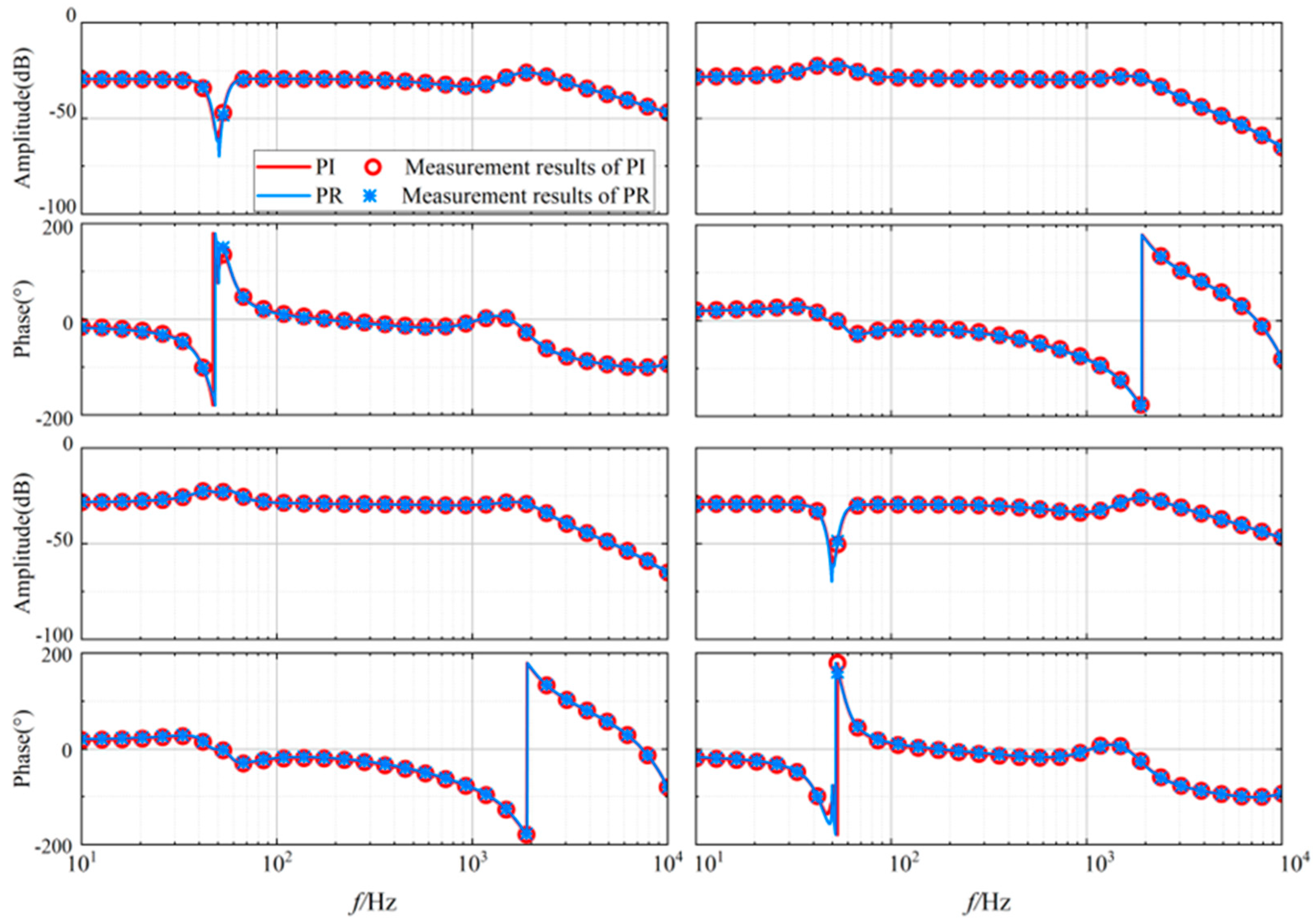
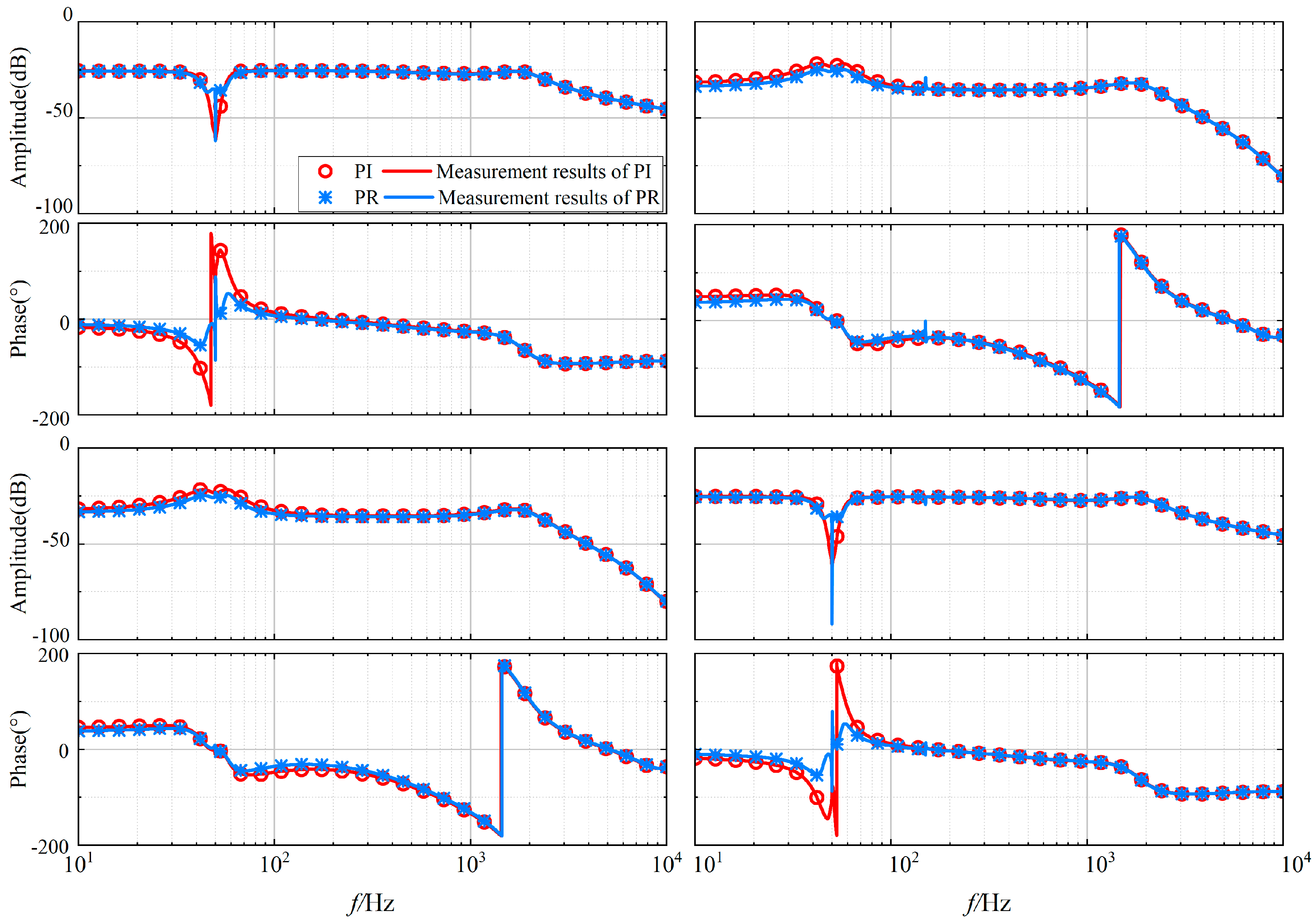
After considering the small disturbance of the phase angle, the Park transform can be expressed as

$$T({\theta }_{PLL}(t))=\left[\begin{array}{ccc}\cos (\Delta {\theta }_{PLL}(t))& \sin (\Delta {\theta }_{PLL}(t))& 0\\ -\sin (\Delta {\theta }_{PLL}(t))& \cos (\Delta {\theta }_{PLL}(t))& 0\\ 0& 0& 1\end{array}\right]T({\theta }_1(t))$$

(26)

After the transformation of the inductor currents i_a, i_b, and i_c of the GCI controlled by PI in the dq domain, the d-axis and q-axis components can be expressed as follows:

$$i_{\mathrm{d}}[f]=\left\{\begin{array}{l}{I}_1\cos {\varphi }_{i1},dc\\ I_{1}sin{\varphi }_{i1}(T_{\mathrm{PLL}}(s_2)G_{\mathrm{vf}}(s){\mathbf{V}}_{\mathrm{p}}+T_{\mathrm{PLL}1}(s_2)G_{\mathrm{vf}}(s_{\mathrm{p}2}){\mathbf{V}}_{\mathrm{p}2})\\ +G_{\mathrm{if}}(s){\mathbf{I}}_{\mathrm{p}}+G_{\mathrm{if}}(s_{\mathrm{p}2}){\mathbf{I}}_{\mathrm{p}2},f=\pm (f_p-f_1)\end{array}\right.$$

(27)

$$i_{\mathrm{q}}[f]=\left\{\begin{array}{l}{I}_{1}sin{\varphi }_{i1},dc\\ -I_1\cos {\varphi }_{i1}(T_{\mathrm{PLL}}(s_2)G_{\mathrm{vf}}(s){\mathbf{V}}_{\mathrm{p}}+T_{\mathrm{PLL}1}(s_2)G_{\mathrm{vf}}(s_{\mathrm{p}2}){\mathbf{V}}_{\mathrm{p}2})\\ \pm j(-G_{\mathrm{if}}(s){\mathbf{I}}_{\mathrm{p}}+G_{\mathrm{if}}(s_{\mathrm{p}2}){\mathbf{I}}_{\mathrm{p}2}),f=\pm (f_p-f_1)\end{array}\right.$$

(28)

According to Figure 1c, the current decoupling of the current inner-loop controller and the dq axis can be obtained:

$$\left\{\begin{array}{l}{c}_{\mathrm{d}}=[(G_{\mathrm{vf}}(s_2)v_{\mathrm{dc}}-v_{\mathrm{ref}})H_{\mathrm{v}}(s_2)-i_{\mathrm{d}}]H_{\mathrm{i}}(s_2)-K_{\mathrm{d}}{i}_{\mathrm{q}}\\ c_{\mathrm{q}}=(i_{\mathrm{qref}}-i_{\mathrm{q}})H_{\mathrm{i}}(s_2)+K_{\mathrm{d}}{i}_{\mathrm{d}}\end{array}\right.$$

(29)

Based on Equation (29), the frequency domain representations for c_d and c_q are articulated as follows:

$$c_{\mathrm{d}}[f]=\left\{\begin{array}{l}{c}_{\mathrm{d}0},dc\\ v_{\mathrm{dc}}{G}_{\mathrm{vf}}(s_2)G_{\mathrm{v}}(s_2)H_{\mathrm{i}}(s_2)-i_{\mathrm{d}}(s_2)H_{\mathrm{i}}(s_2)\\ -K_{\mathrm{d}}{i}_{\mathrm{q}}(s_2),f=\pm (f_{\mathrm{p}}-f_1)\end{array}\right.$$

(30)

$$c_{\mathrm{q}}[f]=\left\{\begin{array}{l}{c}_{\mathrm{q}0},dc\\ -i_{\mathrm{q}}(s_2)H_{\mathrm{i}}(s_2)+K_{\mathrm{d}}{i}_{\mathrm{d}}(s_2),f=\pm (f_{\mathrm{p}}-f_1)\end{array}\right.$$

(31)

In the formula, c_d0 = 2·real(c₁); c_q0 = 2·imag(c₁); c₁ = (V₁ + j2πf₁L_fI₁)/(K_pwmv_dcG_del(s₁)) − K_fG_vf(s₁)V₁.

Following the inverse coordinate transformation applied to Formulas (30) and (31), the expression for the a-phase output signal is detailed as follows:

$$c_a[f]=\cos {\theta }_{PLL}[f]\otimes c_{\mathrm{d}}[f]-\sin {\theta }_{PLL}[f]\otimes c_{\mathrm{q}}[f]$$

(32)

As illustrated in Figure 1, Formulas (30) and (31) are integrated into Formula (32). When combined with Formulas (26) to (30), the resulting frequency coupling admittance matrix for the PI-controlled GCI in the dq domain is delineated as follows:

$$\left[\begin{array}{l}{\mathbf{I}}_{\mathrm{p}}\\ {\mathbf{I}}_{\mathrm{p}2}\end{array}\right]=-\left[\begin{array}{cc}{\mathrm{Y}}_{11\text{\_}\mathrm{PI}}& {\mathrm{Y}}_{12\text{\_}\mathrm{PI}}\\ {\mathrm{Y}}_{21\text{\_}\mathrm{PI}}& {\mathrm{Y}}_{22\text{\_}\mathrm{PI}}\end{array}\right]\left[\begin{array}{l}{\mathbf{V}}_{\mathrm{p}}\\ {\mathbf{V}}_{\mathrm{p}2}\end{array}\right]$$

(33)

The correlation coefficients are as follows:

$$\left[\begin{array}{l}{O}_p\\ O_{p1}\end{array}\right]=\left[\begin{array}{l}{v}_{\mathrm{dc}}{G}_{\mathrm{vf}}(s_2)H_{\mathrm{i}}(s_2)+2(c_1+K_{\mathrm{f}}{G}_{\mathrm{vf}}(s_1){\mathbf{V}}_1)\\ v_{\mathrm{dc}}{G}_{\mathrm{vf}}(s_2)H_{\mathrm{i}}(s_2)+2{(c_1+K_{\mathrm{f}}{G}_{\mathrm{vf}}(s_1){\mathbf{V}}_1)}^{*}\end{array}\right]$$

(34)

$$\left\{\begin{array}{l}{W}_i=G_{\mathrm{if}}(s)(-H_{\mathrm{i}}(s_2)\pm j{K}_d)v_{dc}\\ W_{i1}=G_{\mathrm{if}}(s_{\mathrm{p}1})(-H_{\mathrm{i}}(s_2)\mp j{K}_d)v_{dc}\\ W_v=0.5(-I_1\sin {\varphi }_{i1}\pm j{I}_1\cos {\varphi }_{i1})G_{\mathrm{vf}}(s)T_{\mathrm{PLL}}(s_2)v_{dc}\\ W_v^{*}=0.5(-I_1\sin {\varphi }_{i1}\pm j{I}_1\cos {\varphi }_{i1})G_{\mathrm{vf}}(s_{\mathrm{p}1})T_{\mathrm{PLL}1}(s_2)v_{dc}\\ W_{v1}=0.5(-I_1\sin {\varphi }_{i1}\mp j{I}_1\cos {\varphi }_{i1})G_{\mathrm{vf}}(s)T_{\mathrm{PLL}}(s_2)v_{dc}\\ W_{v1}^{*}=0.5(-I_1\sin {\varphi }_{i1}\mp j{I}_1\cos {\varphi }_{i1})G_{\mathrm{vf}}(s_{\mathrm{p}1})T_{\mathrm{PLL}1}(s_2)v_{dc}\end{array}\right.$$

(35)

$$\left\{\begin{array}{l}{X}_{v1}=\{0.5[K_{\mathrm{d}}(I_1\cos {\varphi }_{i1}\pm j{I}_1\sin {\varphi }_{i1})\pm j{c}_{\mathrm{d}0}-c_{\mathrm{q}0}]T_{\mathrm{PLL}}(s_2)+K_{\mathrm{f}}\}{v}_{\mathrm{dc}}{G}_{\mathrm{vf}}(s_{\mathrm{p}1})\\ X_{v2}=0.5[K_{\mathrm{d}}(I_1\cos {\varphi }_{i1}\pm j{I}_1\sin {\varphi }_{i1})\pm j{c}_{\mathrm{d}0}-c_{\mathrm{q}0}]T_{\mathrm{PLL}1}(s_2)v_{\mathrm{dc}}{G}_{\mathrm{vf}}(s_{\mathrm{p}1})\\ X_{v3}=0.5[K_{\mathrm{d}}(I_1\cos {\varphi }_{i1}\mp j{I}_1\sin {\varphi }_{i1})\mp j{c}_{\mathrm{d}0}-c_{\mathrm{q}0}]T_{\mathrm{PLL}}(s_2)v_{\mathrm{dc}}{G}_{\mathrm{vf}}(s_{\mathrm{p}1})\\ X_{v4}=\{0.5[K_{\mathrm{d}}(I_1\cos {\varphi }_{i1}\mp j{I}_1\sin {\varphi }_{i1})\mp j{c}_{\mathrm{d}0}-c_{\mathrm{q}0}]T_{\mathrm{PLL}1}(s_2)+K_{\mathrm{f}}\}{v}_{\mathrm{dc}}{G}_{\mathrm{vf}}(s_{\mathrm{p}1})\end{array}\right.$$

(36)

$$\begin{array}{l}{Y}_{11\text{\_}\mathrm{PI}}=\\ {\displaystyle \frac{\left\{\begin{array}{l}-[s_{\mathrm{p}2}{L}_{\mathrm{f}}-G_{\mathrm{del}}(s_{\mathrm{p}2})K_{\mathrm{PWM}}(0.5F_{\mathrm{i}2}{O}_{\mathrm{p}1}+W_{\mathrm{i}1})][G_{\mathrm{del}}(s)K_{\mathrm{PWM}}(0.5F_{\mathrm{v}}{O}_{\mathrm{p}}+W_{\mathrm{v}}+X_{\mathrm{v}1})\\ -1]-0.5F_{\mathrm{i}2}{O}_{\mathrm{p}}(0.5F_{\mathrm{v}}{O}_{\mathrm{p}1}+W_{\mathrm{v}1}+X_{\mathrm{v}3})G_{\mathrm{del}}(s)G_{\mathrm{del}}(s_{\mathrm{p}2})K_{\mathrm{PWM}}^2\end{array}\right\}}{\begin{array}{c}[s{L}_f-G_{\mathrm{del}}(s)K_{\mathrm{PWM}}(0.5F_{\mathrm{i}}{O}_{\mathrm{p}}+W_{\mathrm{i}})][s_{\mathrm{p}2}{L}_{\mathrm{f}}-G_{\mathrm{del}}(s_{\mathrm{p}2})K_{\mathrm{PWM}}(0.5F_{\mathrm{i}2}{O}_{{\mathrm{p}}_1}+W_{\mathrm{i}1})]\\ -0.25F_{\mathrm{i}2}{O}_{\mathrm{p}}{F}_{\mathrm{i}}{O}_{\mathrm{p}1}{G}_{\mathrm{del}}(s)G_{\mathrm{del}}(s_{\mathrm{p}2})K_{\mathrm{PWM}}^2\end{array}}}\end{array}$$

(37)

$$\begin{array}{l}{Y}_{12\text{\_}\mathrm{PI}}=\\ {\displaystyle \frac{\left\{\begin{array}{c}-[s_{\mathrm{p}2}{L}_{\mathrm{f}}-G_{\mathrm{del}}(s_{\mathrm{p}2})K_{\mathrm{PWM}}(0.5F_{\mathrm{i}2}{O}_{\mathrm{p}1}+W_{\mathrm{i}1})]G_{\mathrm{del}}(s)K_{\mathrm{PWM}}(0.5F_{\mathrm{v}}{O}_{\mathrm{p}}+W_{\mathrm{v}}^{*}+X_{\mathrm{v}2})\\ -0.5F_{\mathrm{i}2}{O}_{\mathrm{p}}[G_{\mathrm{del}}(s_{\mathrm{p}2})K_{\mathrm{PWM}}(0.5F_{\mathrm{v}2}{O}_{\mathrm{p}1}+W_{\mathrm{v}1}^{*}+X_{\mathrm{v}4})-1]G_{\mathrm{del}}(s)K_{\mathrm{PWM}}\end{array}\right\}}{\begin{array}{c}[s{L}_f-G_{\mathrm{del}}(s)K_{\mathrm{PWM}}(0.5F_{\mathrm{i}}{O}_{\mathrm{p}}+W_{\mathrm{i}})][s_{\mathrm{p}2}{L}_{\mathrm{f}}-G_{\mathrm{del}}(s_{\mathrm{p}2})K_{\mathrm{PWM}}(0.5F_{\mathrm{i}2}{O}_{{\mathrm{p}}_1}+W_{\mathrm{i}1})]\\ -0.25F_{\mathrm{i}2}{O}_{\mathrm{p}}{F}_{\mathrm{i}}{O}_{\mathrm{p}1}{G}_{\mathrm{del}}(s)G_{\mathrm{del}}(s_{\mathrm{p}2})K_{\mathrm{PWM}}^2\end{array}}}\end{array}$$

(38)

$$\begin{array}{l}{Y}_{21\text{\_}\mathrm{PI}}=\\ {\displaystyle \frac{\left\{\begin{array}{c}-0.5F_{\mathrm{i}}{O}_{\mathrm{p}1}[G_{\mathrm{del}}(s)K_{\mathrm{PWM}}(0.5F_{\mathrm{v}}{O}_{\mathrm{p}}+W_{\mathrm{v}}+X_{\mathrm{v}1})-1]G_{\mathrm{del}}(s_{\mathrm{p}2})K_{\mathrm{PWM}}\\ -[s{L}_{\mathrm{f}}-(0.5F_{\mathrm{i}}{O}_{\mathrm{p}}+W_{\mathrm{i}})G_{\mathrm{del}}(s)K_{\mathrm{PWM}}](0.5F_{\mathrm{v}}{O}_{\mathrm{p}1}+W_{\mathrm{v}1}+X_{\mathrm{v}3})G_{\mathrm{del}}(s_{\mathrm{p}2})K_{\mathrm{PWM}}\end{array}\right\}}{\begin{array}{c}[s{L}_f-G_{\mathrm{del}}(s)K_{\mathrm{PWM}}(0.5F_{\mathrm{i}}{O}_{\mathrm{p}}+W_{\mathrm{i}})][s_{\mathrm{p}2}{L}_{\mathrm{f}}-G_{\mathrm{del}}(s_{\mathrm{p}2})K_{\mathrm{PWM}}(0.5F_{\mathrm{i}2}{O}_{{\mathrm{p}}_1}+W_{\mathrm{i}1})]\\ -0.25F_{\mathrm{i}2}{O}_{\mathrm{p}}{F}_{\mathrm{i}}{O}_{\mathrm{p}1}{G}_{\mathrm{del}}(s)G_{\mathrm{del}}(s_{\mathrm{p}2})K_{\mathrm{PWM}}^2\end{array}}}\end{array}$$

(39)

$$\begin{array}{l}{Y}_{22\text{\_}\mathrm{PI}}=\\ {\displaystyle \frac{\left\{\begin{array}{l}-[s{L}_f-G_{\mathrm{del}}(s)K_{\mathrm{PWM}}(0.5F_{\mathrm{i}}{O}_{\mathrm{p}}+W_{\mathrm{i}})][G_{\mathrm{del}}(s_{\mathrm{p}2})K_{\mathrm{PWM}}(0.5F_{\mathrm{v}1}{O}_{\mathrm{p}1}+W_{\mathrm{v}1}^{*}+X_{\mathrm{v}4})\\ -1]-0.5F_{\mathrm{i}}{O}_{\mathrm{p}1}(0.5F_{\mathrm{v}1}{O}_{\mathrm{p}}+W_{\mathrm{v}}^{*}+X_{\mathrm{v}2})G_{\mathrm{del}}(s)G_{\mathrm{del}}(s_{\mathrm{p}2})K_{\mathrm{PWM}}^2\end{array}\right\}}{\begin{array}{c}[s{L}_f-G_{\mathrm{del}}(s)K_{\mathrm{PWM}}(0.5F_{\mathrm{i}}{O}_{\mathrm{p}}+W_{\mathrm{i}})][s_{\mathrm{p}2}{L}_{\mathrm{f}}-G_{\mathrm{del}}(s_{\mathrm{p}2})K_{\mathrm{PWM}}(0.5F_{\mathrm{i}2}{O}_{{\mathrm{p}}_1}+W_{\mathrm{i}1})]\\ \hfill -0.25F_{\mathrm{i}1}{O}_{\mathrm{p}}{F}_{\mathrm{i}}{O}_{\mathrm{p}1}{G}_{\mathrm{del}}(s)G_{\mathrm{del}}(s_{\mathrm{p}2})K_{\mathrm{PWM}}^2\hfill \end{array}}}\end{array}$$

(40)

The theoretical model of frequency-coupling admittance for the GCI controlled by phase-domain PR control and dq-domain PI control has been derived above, and its accuracy can be verified through frequency sweep simulation. The validated system parameters are shown in

Table 1. Parameters of GCI.

Parameters	Values	Parameters	Values
Vdc	700 V	Ipv	14.29 A
Vg	220 V	Qref	0 Kvar
Lf	2 mH	Decoupling coefficient Kd	1/350
Cf	20 uF	Voltage feedforward coefficient Kf	1/350
Rf	1 Ω	PI parameter of PLL	0.266/10.99
Rg	0.2 Ω	Voltage loop PI parameter	1.72/228.69
Lg	3 mH	Current loop PI parameter	0.0343/45.714
ωv, ωi	2π·4000	KPWM	0.5

.

To confirm the accuracy of the model derived, MATLAB/Simulink was used to test the output admittance matrix of two GCIs with different domain current controls, as depicted in Figure 2 and Figure 3. The following conclusions can be made:

(1)

Whether or not the VFL (voltage feedforward link) is considered, the frequency-coupled admittance matrix in different domains aligns with the measured values, confirming the theoretical model’s accuracy.

(2)

Under two different domain current controls, irrespective of VFL, the amplitude values of the diagonal elements Y₁₁ and Y₂₂ are similar to those of the non-diagonal elements Y₁₂ and Y₂₁, highlighting the significance of the frequency coupling effect.

(3)

According to Figure 2 and Figure 3, when VFL is included, the admittance models of the two GCIs controlled by different domains are very similar. Without VFL, the models are notably different.

4. Stability Analysis of GCI Controlled by Different Domains

While the stability analysis can be performed using the frequency-coupled admittance matrix and the GNC, the analysis process is complicated. Under the condition that the same phase margin is met, the frequency-coupled admittance matrix can be simplified to a single input–single output (SISO) sequence impedance model, thus simplifying the subsequent stability analysis. The defined simplified SISO sequence impedance model is specified as follows:

$$\left[\begin{array}{l}{\mathbf{V}}_{\mathrm{P}}\\ {\mathbf{V}}_{\mathrm{n}}\end{array}\right]=\left[\begin{array}{cc}{\mathrm{Z}}_{\mathrm{p}}(s)& 0\\ 0& {\mathrm{Z}}_{\mathrm{n}}(s)\end{array}\right]\left[\begin{array}{c}{\mathbf{I}}_{\mathrm{p}}\\ {\mathbf{I}}_n\end{array}\right]$$

(41)

In the formula, Z_p(s) and Z_n(s) denote the positive sequence and negative sequence impedances of the grid-connected inverters, respectively; V_n and I_n are the injected negative sequence disturbance voltage and the respective responses of the negative sequence current.

By simplifying the established frequency-coupled admittance through the grid impedance Z_g, the positive and negative sequence impedances of the inverter are obtained as follows:

$$\left\{\begin{array}{l}{Z}_{\mathrm{p}}(s)={\displaystyle \frac{1}{Y_{11}-\frac{Y_{12}{Y}_{21}{Z}_g(s-2j\omega )}{1+Y_{22}{Z}_g(s-2j2\omega )}}}\\ Z_{\mathrm{n}}(s)=Z_{\mathrm{p}}^{*}(-s)\end{array}\right.$$

(42)

The stability of the GCIs can be analyzed by the ratio of inverter impedance to grid impedance. The positive and negative sequence impedance ratio is defined as follows:

$$Z{R}_{\mathrm{P}}(s)={\displaystyle \frac{Z_{\mathrm{gp}}(s)}{Z_{\mathrm{p}}(s)}};Z{R}_{\mathrm{n}}(s)={\displaystyle \frac{Z_{\mathrm{gn}}(s)}{Z_{\mathrm{n}}(s)}}$$

(43)

In the formula, Z_gp(s) and Z_gn(s) are the positive sequence impedance and negative sequence impedance of the power grid, respectively; Z_gp(s) = Z_gn(s) = (R_g + sL_g)||[R_f + 1/(sC_f)].

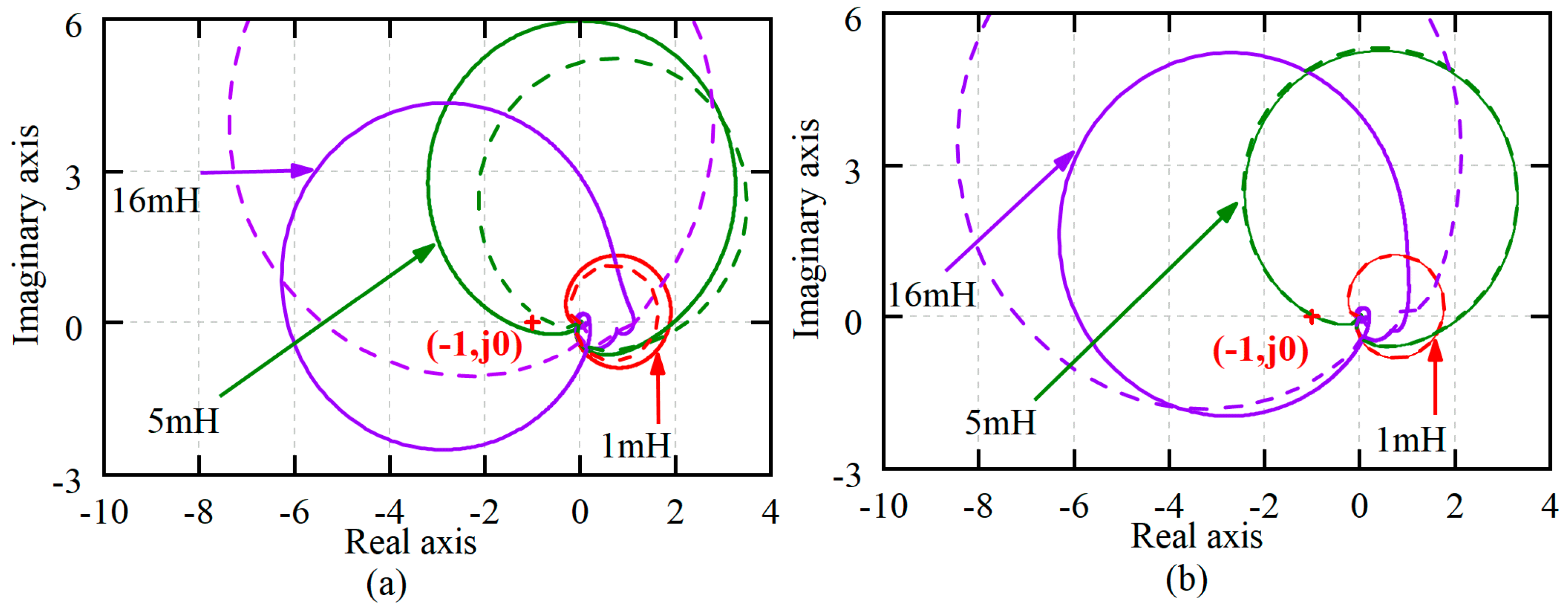
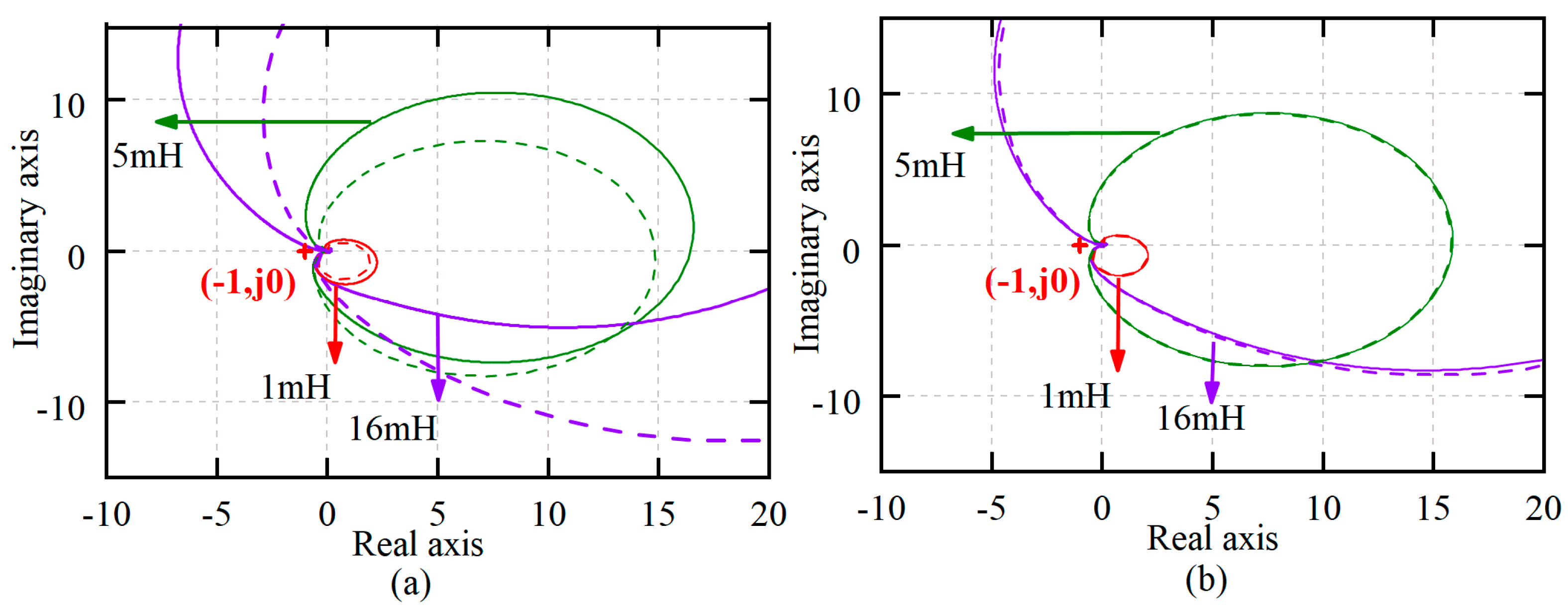
4.1. Influence of Power Grid Strength on Stability

We explore how the strength of the power grid affects the stability of GCIs under various domain control scenarios, given PLL bandwidth BW_PLL = 20 Hz, DC voltage loop control bandwidth BW_v = 30 Hz, current loop control bandwidth BW_ic = 600 Hz. The Nyquist diagrams illustrating the effects of changes in the grid impedance L_g are displayed in Figure 4 and Figure 5.

In Figure 4a, when the grid impedance is 1 mH and 5 mH, the Nyquist plots for the positive sequence impedance ratio ZR_p(s) and the negative sequence impedance ratio ZR_n(s) do not encompass the point (−1, j0). However, when the grid impedance increases to 16 mH, the Nyquist diagrams of the positive sequence impedance ratio ZR_p(s) encircle the point (−1, j0).

In Figure 4b, when the grid impedance is 1 mH, 5 mH, and 16 mH, the Nyquist plots for ZR_p(s) and ZR_n(s) do not encompass the point (−1, j0). Therefore, the stability of GCIs using time-domain PR control is slightly better than that of inverters using dq-domain PI control under weak grid conditions, and their performances are very close.

In Figure 5a, when the grid impedance is 1 mH, the Nyquist plots for ZR_p(s) and ZR_n(s) do not encompass the point (−1, j0). When the grid impedance is 45 mH and 5 mH, the Nyquist diagrams of ZR_p(s) and ZR_n(s) encompass the point (−1, j0).

In Figure 5b, when the network impedance is 1 mH and 5 mH, the Nyquist diagrams for ZR_p(s) and ZR_n(s) do not encompass the point (−1, j0). However, when the grid impedance is 45 mH, the Nyquist diagrams for ZR_p(s) and ZR_n(s) encompass the point (−1, j0). By comparison with Figure 5, it is evident that considering power grid voltage feedforward control decreases the stability of GCIs controlled by PR control in the time domain and PI control in the dq domain when connected to a weak power grid.

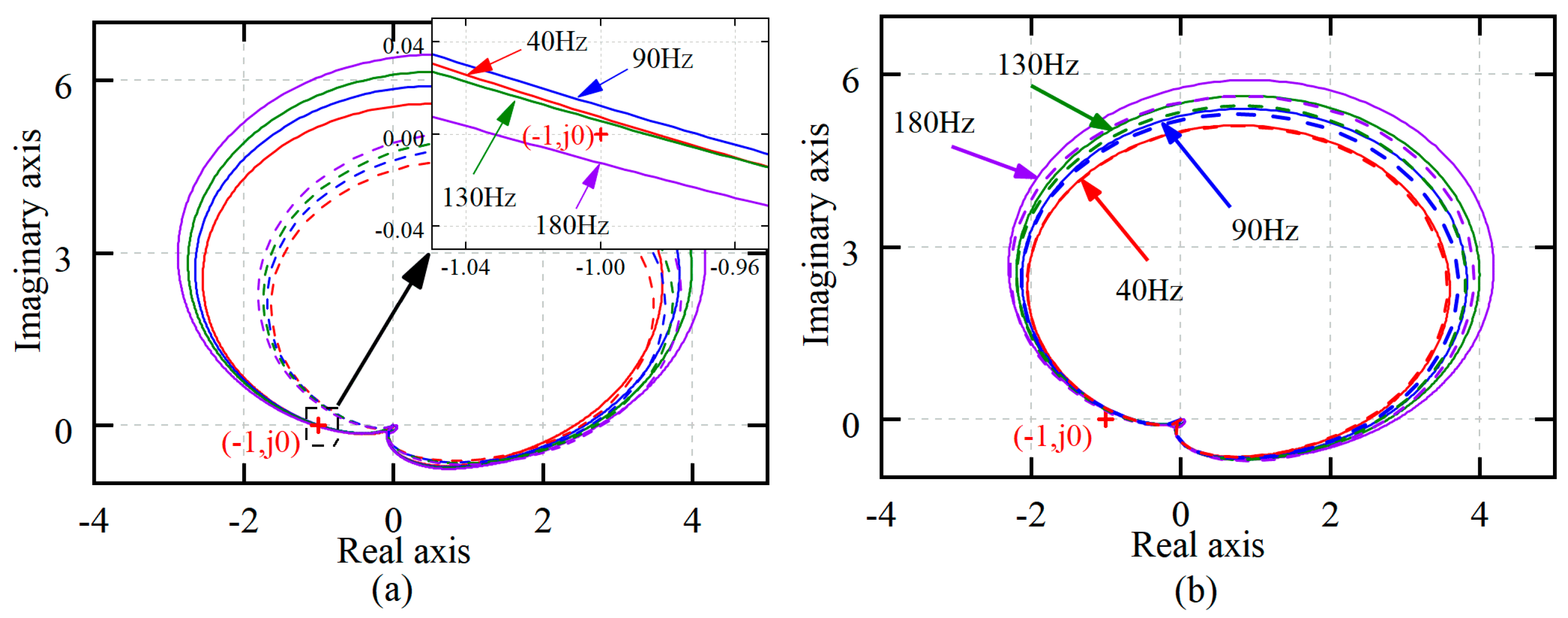
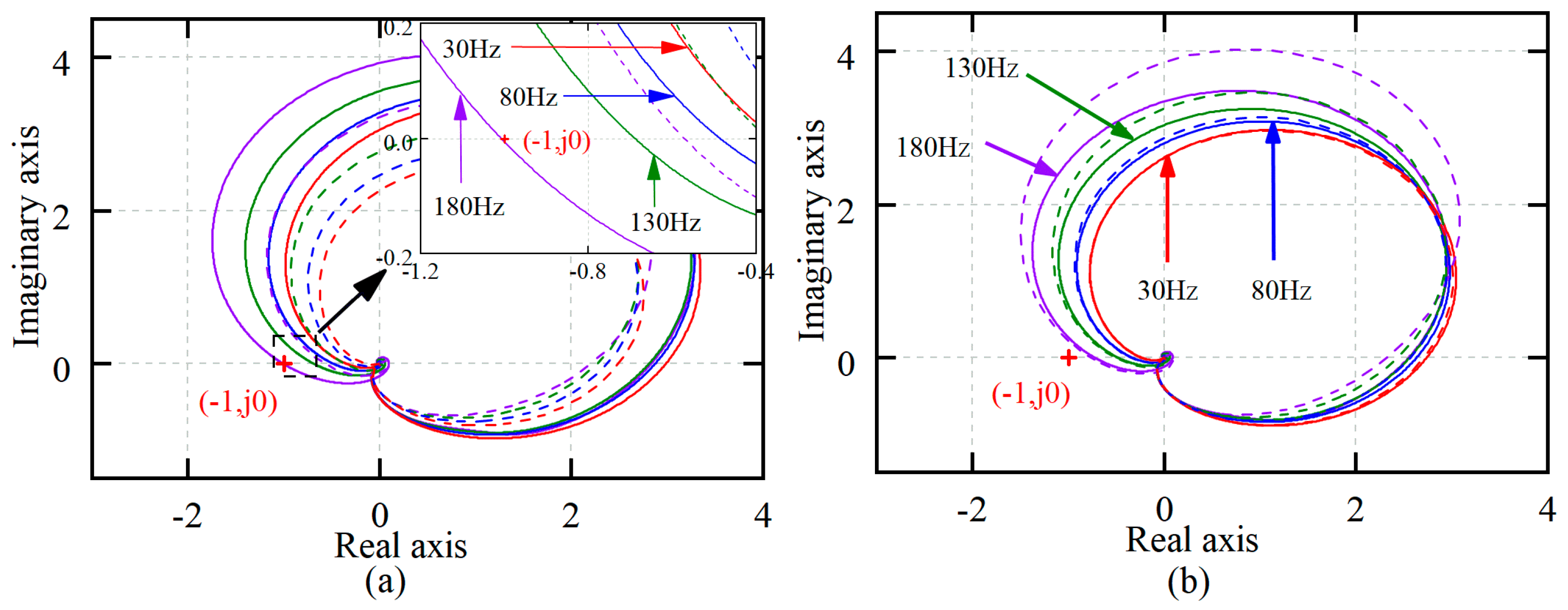
4.2. Impact of PLL Bandwidth BW_PLL

To investigate the impact of PLL bandwidth BW_PLL on the stability of grid-connected inverters under various domain controls, the DC voltage loop control bandwidth BW_v = 30 Hz, current loop control bandwidth BW_ic = 600 Hz, and grid side inductance L_g = 4 mH are specified. The Nyquist diagrams depicting changes in the PLL bandwidth BW_PLL are displayed in Figure 6 and Figure 7.

In Figure 6a, the Nyquist diagrams for the positive sequence impedance ratio ZR_p(s) and negative sequence impedance ratio ZR_n(s) do not encircle the point (−1, j0) when the PLL bandwidth BW_PLL is set at 40 Hz, 90 Hz, and 130 Hz, confirming system stability. However, as the PLL bandwidth increases to 180 Hz, the Nyquist diagram for the positive sequence impedance ratio ZR_p(s) encircles the point (−1, j0), indicating potential system instability.

In Figure 6b, the Nyquist diagrams for the positive sequence impedance ratio ZR_p(s) and the negative sequence impedance ratio ZR_n(s) do not encircle the point (−1, j0) at PLL bandwidths BW_PLL of 40 Hz, 90 Hz, 130 Hz, and 180 Hz, indicating that the system remains stable.

In Figure 7a,b, when the PLL bandwidth BW_PLL is 40 Hz, 90 Hz, 130 Hz, and 180 Hz, the Nyquist diagrams for ZR_p(s) and ZR_n(s) do not encircle the point (−1, j0). This suggests that the system is stable.

Figure 6 and Figure 7 demonstrate that, without implementing voltage feedforward control, the stability of the grid-connected inverters under both control modes declines as the PLL bandwidth increases. However, the stability of the time-domain PR-controlled GCI is marginally better than that of the dq-domain PI-controlled GCI, though their performances are nearly equivalent.

In addition, when voltage feedforward control is introduced, the stability of grid-connected inverters using both time-domain PR control and dq-domain PI control is reduced, particularly at high PLL bandwidths, which may lead to instability.

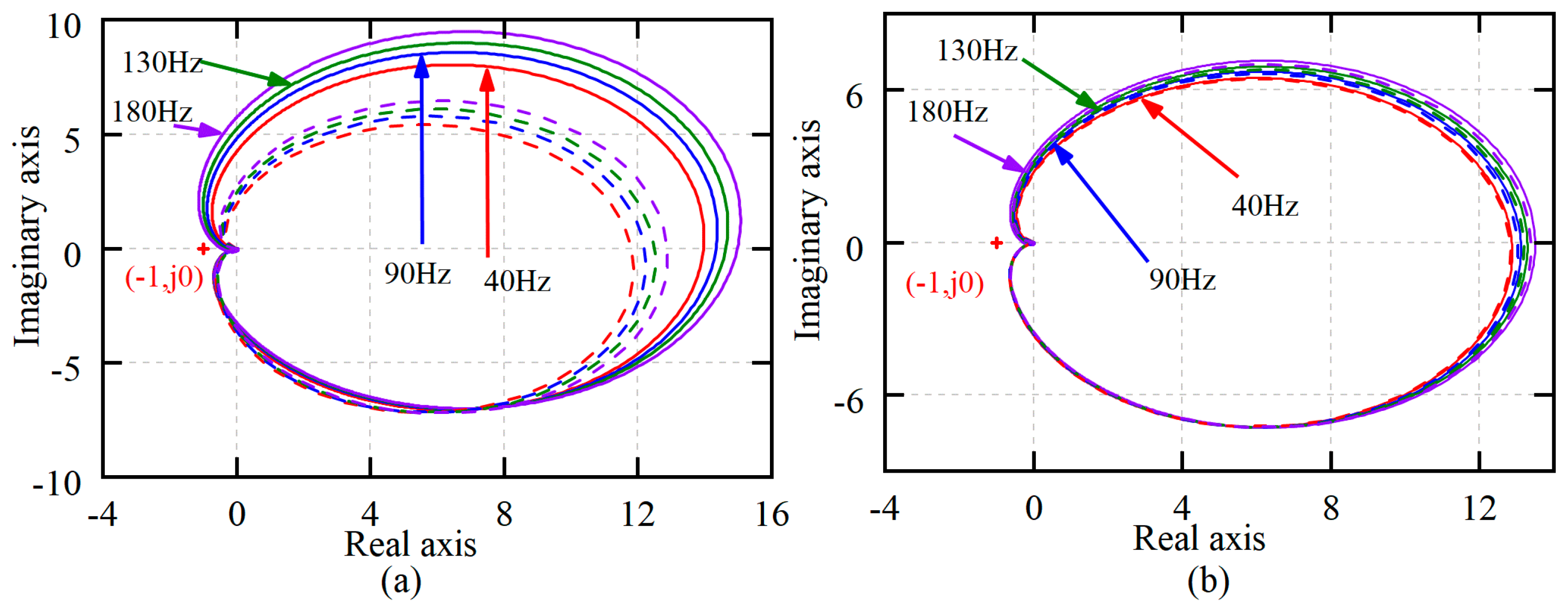
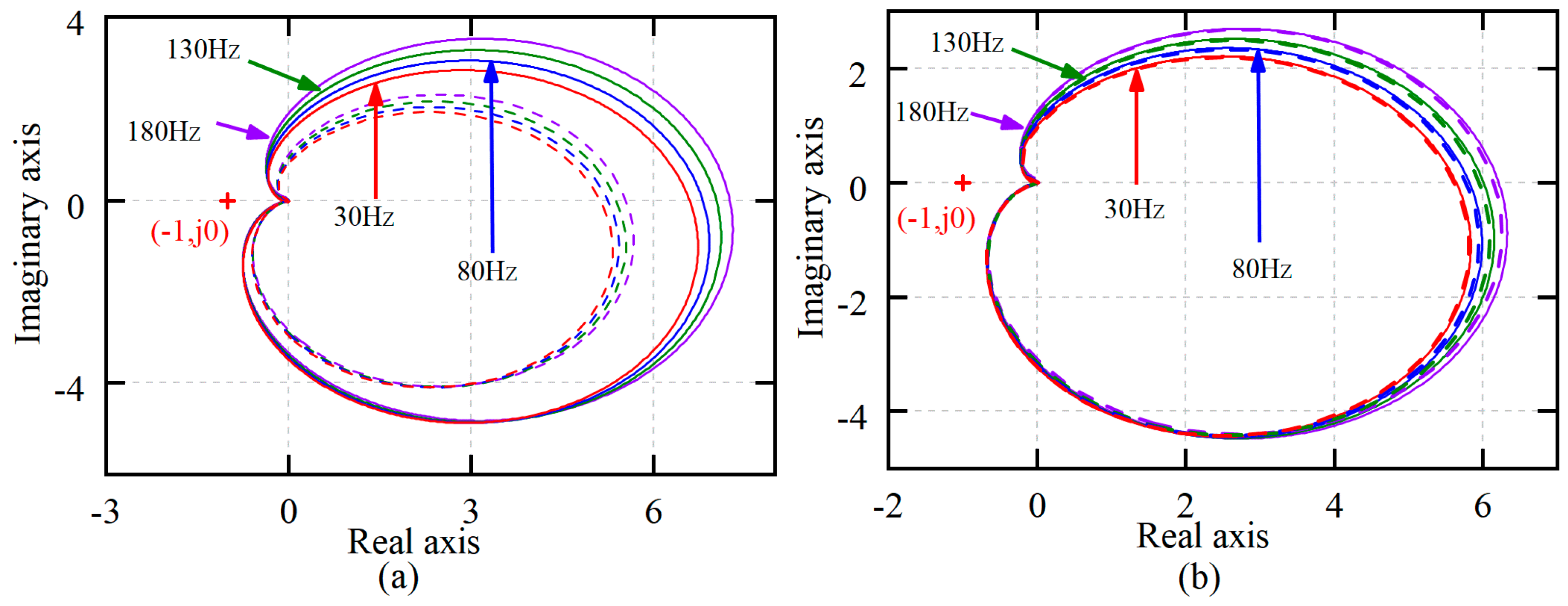
4.3. Influence of DC Voltage Loop Bandwidth BWv

In order to study the influence of DC voltage loop bandwidth BWv on the stability of GCIs under different domain controls, given PLL bandwidth BW_PLL = 20 Hz, current loop control bandwidth BWic = 600 Hz, and grid side inductance Lg = 2 mH, the Nyquist diagrams when the DC voltage loop bandwidth BWv is changed are shown in Figure 8 and Figure 9.

In Figure 8a, when the outer loop bandwidth BW_v is 30 Hz, 80 Hz, and 130 Hz, the Nyquist diagrams for the positive sequence impedance ratio ZR_p(s) and the negative sequence impedance ratio ZR_n(s) do not encircle the point (−1, j0). However, at an outer loop bandwidth of 180 Hz, the Nyquist diagrams of ZR_p(s) encircle the point (−1, j0), indicating instability.

In Figure 8b, at outer loop bandwidths of 30 Hz, 80 Hz, 130 Hz, and 180 Hz, the Nyquist diagrams for both ZR_p(s) and ZR_n(s) do not surround point (−1, j0), suggesting stability across these settings.

In Figure 9a,b, when the outer loop bandwidth BW_v is 40 Hz, 90 Hz, 130 Hz, and 180 Hz, the Nyquist diagrams for ZR_p(s) and ZR_n(s) do not encircle the point (−1, j0).

As seen from Figure 8 and Figure 9, when voltage feedforward control is not considered, the stability of GCIs under both control modes decreases as the outer loop bandwidth BW_v increases.

Additionally, with the introduction of voltage feedforward control, the stability of inverters using both time-domain PR control and dq-domain PI control is reduced, particularly at high outer loop bandwidths, which may lead to instability.

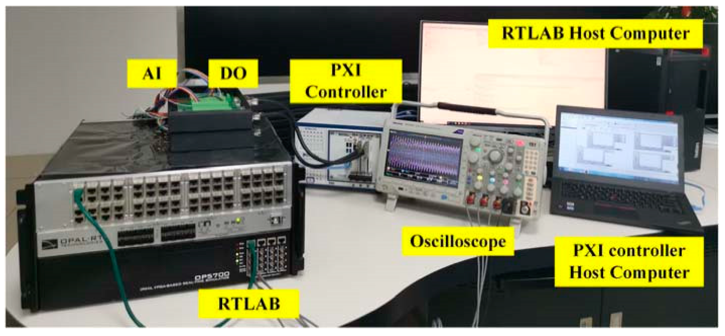
5. Experimental Verification

To further validate the accuracy of the preceding theoretical analysis and conclusions, a stability experiment of the GCI system was conducted on the RTLAB experimental platform, as depicted in Figure 10. The experimental parameters were consistent with those used in the theoretical analysis. The main circuit, including the DC line, capacitor, inductor, resistor, and power supply, was built on the RTLAB platform, and the control part was completed by the digital control platform. The specific parameters of the system are shown in Table 1.

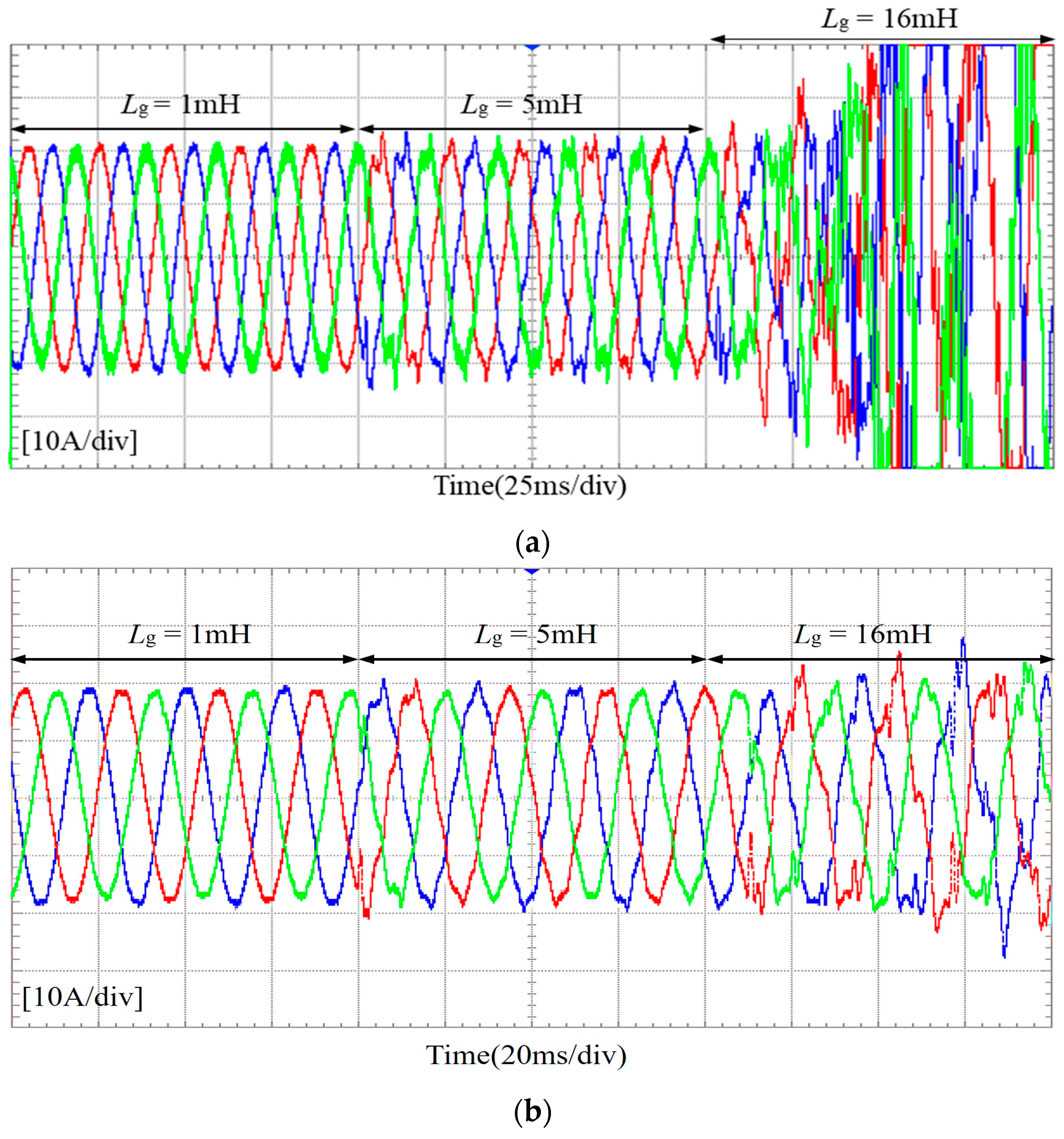
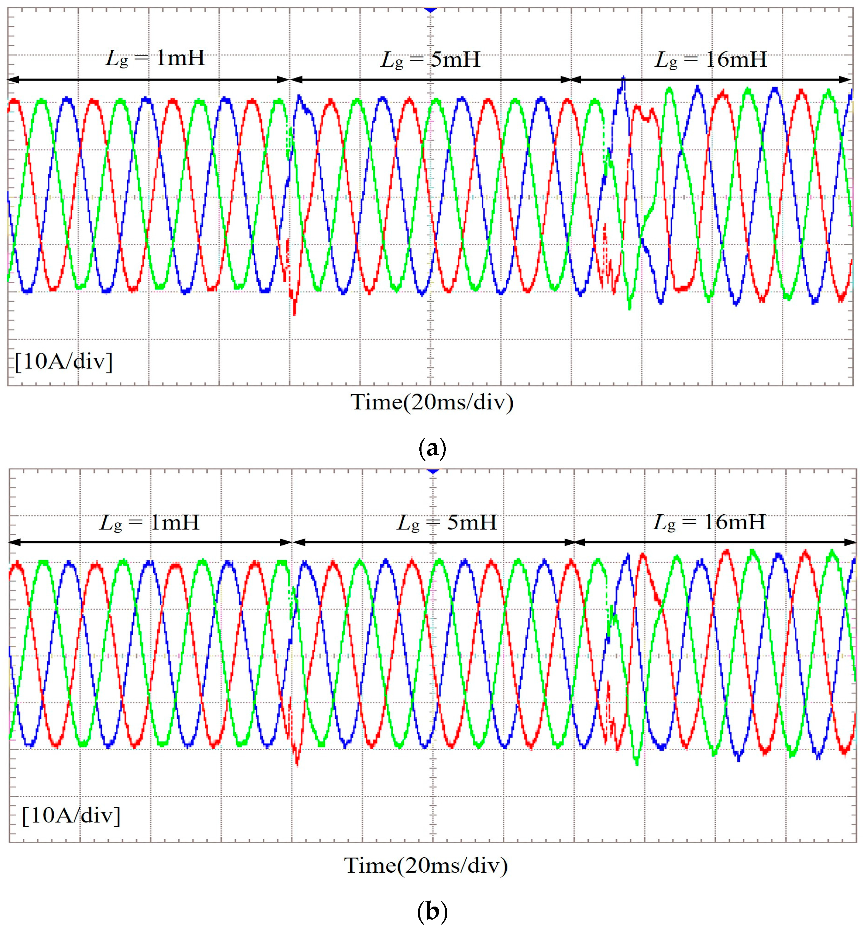
5.1. Influence of Power Grid Strength on the Stability of GCI Systems

GCI grid-connected currents controlled by two different domains under various power grid intensities are depicted in Figure 11 with voltage feedforward control considered.

As shown in Figure 11a, with an inductance Lg = 1 mH, the GCI system controlled by PI in the dq domain is stable. When Lg = 5 mH, the grid-connected current exhibits waveform distortion and harmonic oscillation, indicating poor system stability. When Lg = 16 mH, the grid-connected current diverges significantly, leading to serious instability. Figure 11b shows that with Lg = 1 mH and 5 mH, the GCI system controlled by phase-domain PR is stable; when Lg = 16 mH, it also shows waveform distortion and harmonic oscillation, reflecting poor system stability.

GCI grid-connected currents controlled by two different domains under varying power grid intensities are shown in Figure 12 with voltage feedforward control not considered.

It can be observed from Figure 12 that when the grid inductance L_g is 1 mH, 5 mH, and 16 mH, the GCI systems controlled by PI in the dq domain and PR in the phase domain are both stable.

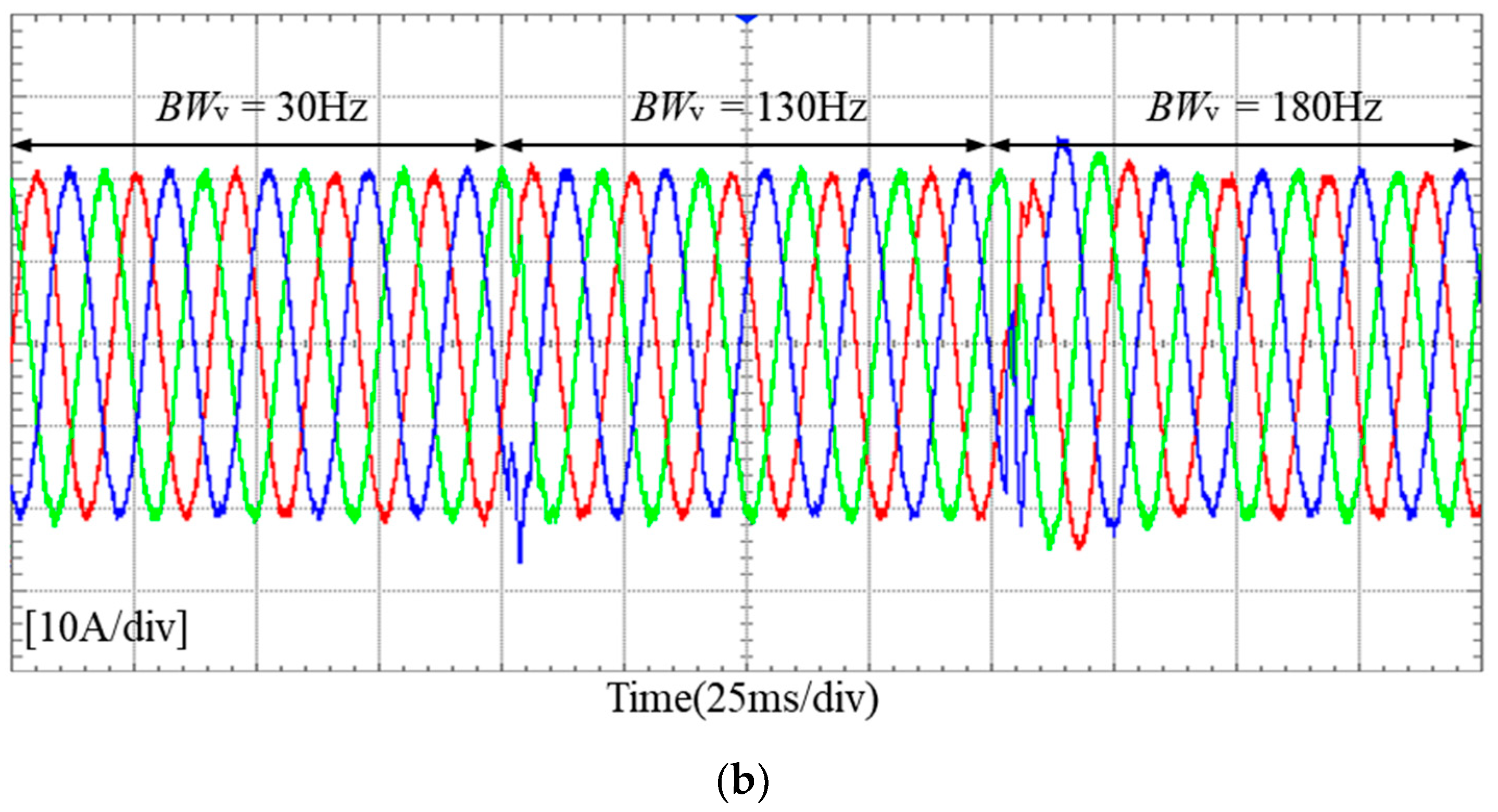
5.2. Influence of Voltage Outer Loop Bandwidth on the Stability of GCI Systems

With voltage feedforward control considered, GCI grid-connected currents controlled by two different domains under different voltage outer loop bandwidths are shown in Figure 13.

From Figure 13a, it can be seen that when the voltage outer loop bandwidth BW_v = 30 Hz and 130 Hz, the GCI system controlled by PI in the dq domain maintains stability; however, when the bandwidth of the voltage outer loop BW_v = 180 Hz, the grid-connected current of the GCI system controlled by PI in the dq domain diverges significantly, leading to system instability. As shown in Figure 13b, the GCI system controlled by phase-domain PR remains stable at bandwidths of 30 Hz, 130 Hz, and 180 Hz.

With voltage feedforward control not considered, GCI grid-connected currents controlled by two different domains with varying voltage outer loop bandwidths are depicted in Figure 14.

According to Figure 14, when the voltage outer loop bandwidth BW_v = 30 Hz, 130 Hz, and 180 Hz, the GCI system controlled by PI control in the dq domain and PR control in the phase domain remains stable.

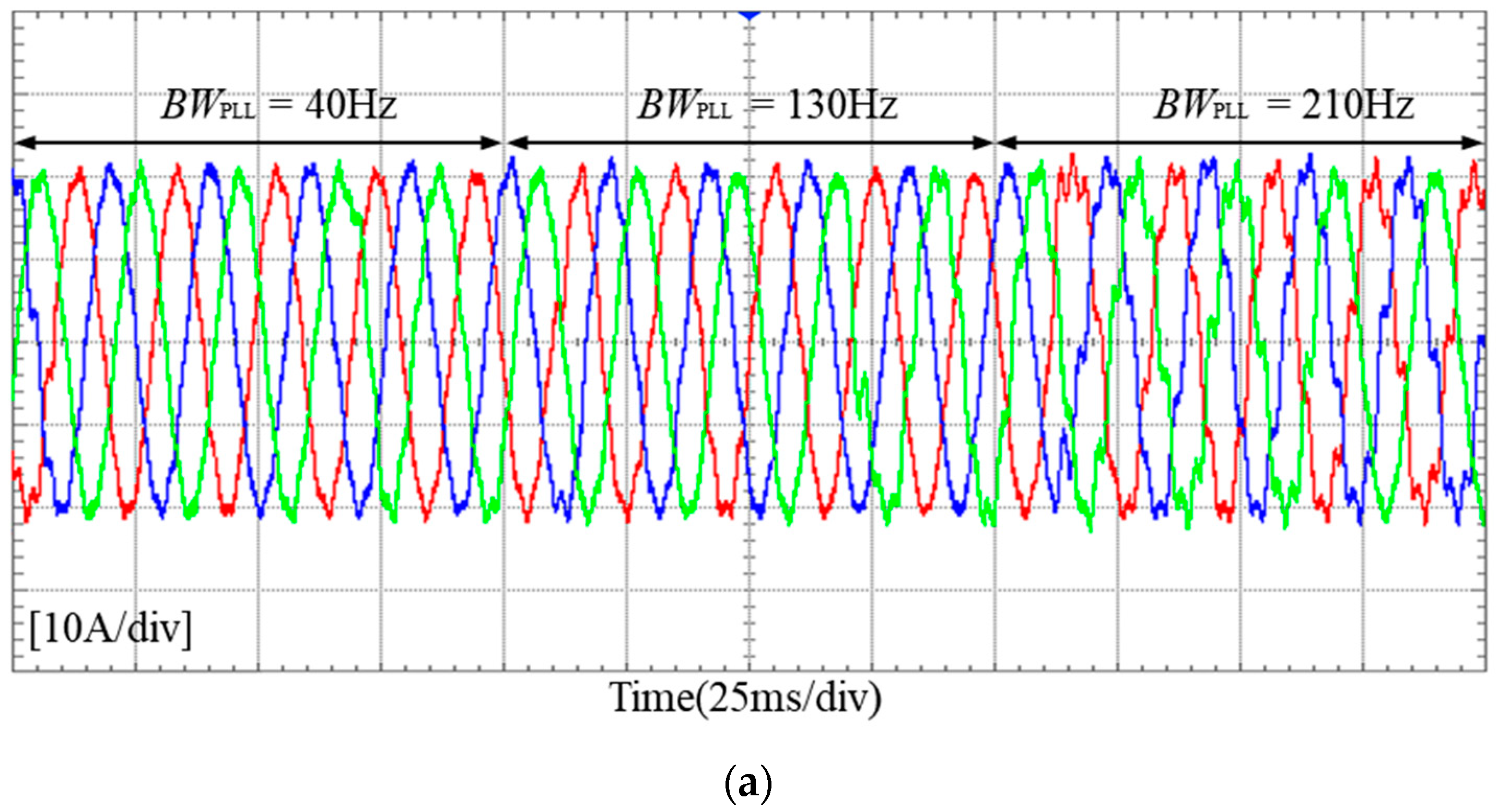
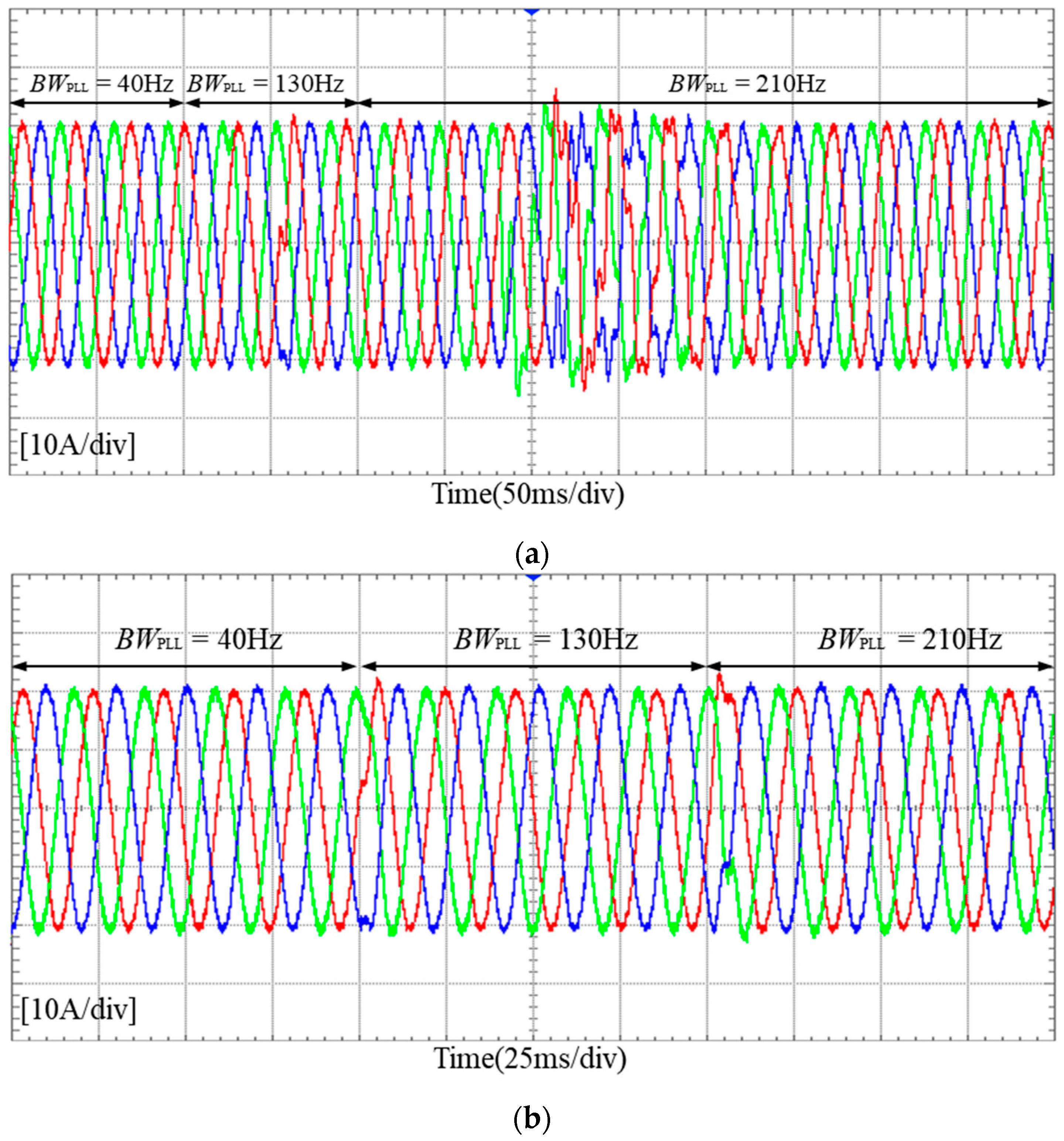
5.3. Influence of PLL Bandwidth on the Stability of GCI Systems

With voltage feedforward control considered, GCI grid-connected currents controlled by two different domains under varying PLL bandwidths are illustrated in Figure 15.

As shown in Figure 15a, when the PLL bandwidth BW_v = 40 Hz and 130 Hz, the GCI system controlled by phase-domain PR remains stable; however, at a PLL bandwidth of 210 Hz, the grid-connected current exhibits significant waveform distortion and harmonic oscillation, indicating poor system stability. Figure 15b reveals that with PLL bandwidths of 40 Hz, 130 Hz, and 180 Hz, the GCI system controlled by phase-domain PR is stable.

With voltage feedforward control not considered, GCI grid-connected currents controlled by two different domains under various PLL bandwidths are displayed in Figure 16.

According to Figure 16, when the PLL bandwidth BW_v = 40 Hz, 130 Hz, and 180 Hz, the GCI systems controlled by PI control in the dq domain and PR control in the phase domain remain stable.

6. Conclusions

In the case of voltage feedforward control, the frequency-coupled admittance models of phase-domain PR control and dq-domain PI control were established using the harmonic linearization method. The stability of the GCI system under these two current control methods was compared and analyzed based on the equivalent positive and negative sequence impedance and the traditional Nyquist criterion, yielding the following conclusions:

(1)

Regardless of whether voltage feedforward control is considered, adopting PI control and PR current control, considering the frequency coupling characteristics, will establish a more accurate frequency-coupled admittance model.

(2)

With voltage feedforward control, the admittance characteristics of GCI systems controlled by PI and PR are similar. Without voltage feedforward control, the frequency-coupled admittance models of GCI systems under PI and PR control differ significantly in the baseband.

(3)

To enhance the stability of the GCI system, the bandwidths of the phase-locked loop and the voltage outer loop should be minimized, provided that dynamic performance requirements are met.

(4)

In conditions of high penetration, voltage feedforward control diminishes the stability of GCI systems under both PI and PR control, increasing the likelihood of instability. Moreover, if a GCI system controlled by PI shows insufficient stability, employing PR control can marginally enhance stability without altering the mainline parameters and control settings.

References

1. Li, Z.; Guo, Q.; Sun, H.; Wang, J.; Xu, Y.; Fan, M. A Distributed Transmission-Distribution-Coupled Static Voltage Stability Assessment Method Considering Distributed Generation. IEEE Trans. Power Syst. 2018, 33, 2621–2632. [Google Scholar] [CrossRef]
2. Verma, P.; Seethalekshmi, K.; Dwivedi, B. A Self-Regulating Virtual Synchronous Generator Control of Doubly Fed Induction Generator-Wind Farms. IEEE Can. J. Electr. Comput. Eng. 2023, 46, 35–43. [Google Scholar] [CrossRef]
3. Li, G.; Chen, Y.; Luo, A.; Wang, H. An Enhancing Grid Stiffness Control Strategy of STATCOM/BESS for Damping Sub-Synchronous Resonance in Wind Farm Connected to Weak Grid. IEEE Trans. Ind. Inform. 2020, 16, 5835–5845. [Google Scholar] [CrossRef]
4. Sewdien, V.; Preece, R.; Torres, J.R.; van der Meijden, M. Systematic Procedure for Mitigating DFIG-SSR Using Phase Imbalance Compensation. IEEE Trans. Sustain. Energy 2022, 13, 101–110. [Google Scholar] [CrossRef]
5. Zhou, J.Z.; Ding, H.; Fan, S.; Zhang, Y.; Gole, A.M. Impact of Short-Circuit Ratio and Phase-Locked-Loop Parameters on the Small-Signal Behavior of a VSC-HVDC Converter. IEEE Trans. Power Deliv. 2014, 29, 2287–2296. [Google Scholar] [CrossRef]
6. Chen, X.; Wang, Y.; Gong, C.; Sun, J. Overview of Stability Research for Grid-Connected Inverters Based on Impedance Analysis Method. Proc. CSEE 2018, 38, 2082–2094. [Google Scholar]
7. Sun, J. Impedance-Based Stability Criterion for Grid-Connected Inverters. IEEE Trans. Power Electron. 2011, 26, 3075–3078. [Google Scholar] [CrossRef]
8. Wang, X.; Harnefors, L.; Blaabjerg, F. Unified Impedance Model of Grid-Connected Voltage-Source Converters. IEEE Trans. Power Electron. 2018, 33, 1775–1787. [Google Scholar] [CrossRef]
9. Qian, Q.; Xie, S.; Xu, J.; Xu, K.; Bian, S.; Zhong, N. Output Impedance Modeling of Single-Phase Grid-Tied Inverters with Capturing the Frequency-Coupling Effect of PLL. IEEE Trans. Power Electron. 2020, 35, 5479–5495. [Google Scholar] [CrossRef]
10. Nian, H.; Liao, Y.; Li, M.; Sun, D.; Xu, Y.; Hu, B. Impedance Modeling and Stability Analysis of Three-Phase Four-Leg Grid-Connected Inverter Considering Zero-Sequence. IEEE Access 2021, 9, 83676–83687. [Google Scholar] [CrossRef]
11. Du, Y.; Zhao, H.; Yang, X.; Jiang, W.; Su, J. Sequence Impedance Modeling of Virtual Synchronous Generator Considering Frequency Coupling Effect. J. Power Supply 2020, 18, 42–49. [Google Scholar]
12. Bakhshizadeh, M.K.; Wang, X.; Blaabjerg, F.; Hjerrild, J.; Kocewiak, Ł.; Bak, C.L.; Hesselbæk, B. Couplings in Phase Domain Impedance Modeling of Grid-Connected Converters. IEEE Trans. Power Electron. 2016, 31, 6792–6796. [Google Scholar] [CrossRef]
13. Heng, N.; Yunyang, X.; Liang, C.; Guanghui, L. Frequency Coupling Characteristic Modeling of Grid-connected Inverter and System Stability Analysis. Proc. CSEE 2019, 39, 1421–1432. [Google Scholar]
14. Xie, Z.; Wu, W.; Chen, Y.; Gong, W. Admittance-based stability comparative analysis of grid-connected inverters with direct power control and closed-loop current control. IEEE Trans. Ind. Electron. 2021, 68, 8333–8344. [Google Scholar] [CrossRef]
15. Yang, Z.; Shah, C.; Chen, T.; Yu, L.; Joebges, P.; De Doncker, R.W. Stability investigation of three-phase grid-tied PV inverter systems using impedance models. IEEE J. Emerg. Sel. Top. Power Electron. 2022, 10, 2672–2684. [Google Scholar] [CrossRef]
16. Manoloiu, A.; Pereira, H.A.; Teodorescu, R.; Bongiorno, M.; Eremia, M.; Silva, S.R. Comparison of PI and PR current controllers applied on two-level VSC-HVDC transmission system. In Proceedings of the 2015 IEEE Eindhoven PowerTech, Eindhoven, The Netherlands, 28 June–2 July 2015; pp. 1–5. [Google Scholar]
17. Wen, B.; Dong, D.; Boroyevich, D.; Burgos, R.; Mattavelli, P.; Shen, Z. Impedance-Based Analysis of Grid-Synchronization Stability for Three-Phase Paralleled Converters. IEEE Trans. Power Electron. 2016, 31, 26–38. [Google Scholar] [CrossRef]
18. Xie, Z.; Chen, Y.; Wu, W.; Xu, Y.; Wang, H.; Guo, J.; Luo, A. Modeling and Control Parameters Design for Grid-Connected Inverter System Considering the Effect of PLL and Grid Impedance. IEEE Access 2020, 8, 40474–40484. [Google Scholar] [CrossRef]
19. Liu, W.; Xie, X.; Zhang, X.; Li, X. Frequency-Coupling Admittance Modeling of Converter-Based Wind Turbine Generators and the Control-Hardware-in-the-Loop Validation. IEEE Trans. Energy Convers. 2019, 35, 425–433. [Google Scholar] [CrossRef]
20. Wu, X.Q.; Wang, Y.C.; Chen, X.; Chen, J.; He, G.Q. Sequence Impedance Model and Interaction Stability Research of Three-phase Grid-connected Inverters with Considering Coupling Effects. Proc. CSEE 2020, 40, 1605–1616. [Google Scholar]
21. Wang, H.; Xie, Z.; Chen, Y.; Wu, W.; Zhu, Z.; Gao, J. Stability enhancement control strategy for grid-connected wind power system based on composite feedforward damping. Int. J. Electr. Power Energy Syst. 2024, 158, 109908. [Google Scholar] [CrossRef]
22. Gao, S.; Zhao, H.; Wang, P.; Gui, Y.; Terzija, V.; Blaabjerg, F. Comparative study of symmetrical controlled grid-connected inverters. IEEE Trans. Power Electron. 2022, 37, 3954–3968. [Google Scholar] [CrossRef]
23. Wang, K.; Yuan, X.; Wang, H.; Zhang, Y.; Wu, X. Two causes of the inverter-based grid-connected system instability in weak grids. Power Syst. Technol. 2023, 47, 1230–1242. [Google Scholar]
24. Xie, Z.; Chen, Y.; Wu, W.; Gong, W.; Guerrero, J.M. Stability enhancing voltage feed-forward inverter control method to reduce the effects of phase-locked loop and grid impedance. IEEE J. Emerg. Sel. Top. Power Electron. 2021, 9, 3000–3009. [Google Scholar] [CrossRef]
25. Li, Y.; Zhiyuan, H.; Hui, P.; Yang, Y.; Weiying, H. High frequency stability analysis and suppression strategy of MMC-HVDC systems (Part I): Stability analysis. Proc. CSEE 2021, 41, 5842–5855. [Google Scholar]
26. Zmood, D.N.; Holmes, D.G. Stationary frame current regulation of PWM inverters with zero steady-state error. IEEE Trans. Power Electron. 2003, 18, 814–822. [Google Scholar] [CrossRef]
Figure 1. GCI system topology and control block diagram. (a) GCI system topology; (b) GCI system controlled by PI in the dq domain; (c) GCI system with PR control in the time domain.
Applsci 14 09026 g001aApplsci 14 09026 g001b
Figure 2. The frequency-coupled admittance model of GCI without considering voltage feedforward.
Applsci 14 09026 g002
Figure 3. Frequency-coupled admittance model of GCI considering voltage feedforward.
Applsci 14 09026 g003
Figure 4. Nyquist diagram with Lg change when voltage feedforward control is considered. (a) PI control; (b) PR control.
Applsci 14 09026 g004
Figure 5. Nyquist diagram when Lg changes without considering voltage feedforward control. (a) PI control. (b)PR control.
Applsci 14 09026 g005
Figure 6. Nyquist diagram with BWPLL changes when voltage feedforward control is considered. (a) PI control. (b) PR control.
Applsci 14 09026 g006
Figure 7. Nyquist diagram with BWPLL changes when voltage feedforward control is considered. (a) PI control. (b) PR control.
Applsci 14 09026 g007
Figure 8. Nyquist diagram with BWv change when voltage feedforward is considered. (a) PI control. (b) PR control.
Applsci 14 09026 g008
Figure 9. Nyquist diagram with BWv change without considering voltage feedforward. (a) PI control. (b) PR control.
Applsci 14 09026 g009
Figure 10. RTLAB experimental platform.
Applsci 14 09026 g010
Figure 11. Grid-connected current waveform under different power grid strengths, considering voltage feedforward. (a) The dq-domain PI-controlled GCI system; (b) the phase-domain PR-controlled GCI system.
Applsci 14 09026 g011
Figure 12. Grid-connected current waveform under different power grid strengths without considering voltage feedforward. (a) The dq-domain PI-controlled GCI system; (b) the phase-domain PR-controlled GCI system.
Applsci 14 09026 g012
Figure 13. Grid-connected current waveform with different outer loop bandwidths considering voltage feedforward. (a) The dq-domain PI-controlled GCI system; (b) the phase-domain PR-controlled GCI system.
Applsci 14 09026 g013aApplsci 14 09026 g013b
Figure 14. Grid-connected current waveform at different outer loop bandwidths without considering voltage feedforward. (a) The dq-domain PI-controlled GCI system; (b) the phase-domain PR-controlled GCI system.
Applsci 14 09026 g014aApplsci 14 09026 g014b
Figure 15. Grid-connected current waveform under different PLL bandwidths considering voltage feedforward. (a) The dq-domain PI-controlled GCI system; (b) the phase-domain PR-controlled GCI system.
Applsci 14 09026 g015aApplsci 14 09026 g015b
Figure 16. Grid-connected current waveform under different PLL bandwidths without considering voltage feedforward. (a) The dq-domain PI-controlled GCI system; (b) the phase-domain PR-controlled GCI system.
Applsci 14 09026 g016