Abstract
In this paper, we present an analysis of the effectiveness of various machine learning algorithms in classifying astronomical objects using data from the third release (DR3) of the Gaia space mission. The dataset used includes spectral information from the satellite’s red and blue spectrophotometers. The primary goal is to achieve reliable classification with high confidence for symbiotic stars, planetary nebulae, and red giants. Symbiotic stars are binary systems formed by a high-temperature star (a white dwarf in most cases) and an evolved star (Mira type or red giant star); their spectra varies between the typical for these objects (depending on the orbital phase of the object) and present emission lines similar to those observed in PN spectra, which is the reason for this first selection. Several classification algorithms are evaluated, including Random Forest (RF), Support Vector Machine (SVM), Artificial Neural Networks (ANN), Gradient Boosting (GB), and Naive Bayes classifier. The evaluation is based on different metrics such as Precision, Recall, F1-Score, and the Kappa index. The study confirms the effectiveness of classifying the mentioned stars using only their spectral information. The models trained with Artificial Neural Networks and Random Forest demonstrated superior performance, surpassing an accuracy rate of 94.67%.
1. Introduction
Gaia, a project of the European Space Agency (ESA), began scientific operations in mid-2014, after a successful commissioning phase. Gaia’s primary scientific aim is to scrutinize the kinematic, dynamic, chemical, and evolutionary status of the Milky Way galaxy. Through continuous sky scanning, Gaia gathers astrometric, photometric, and spectroscopic data from an extensive set of stars. The mission’s ability to cover an extended region in space at many times makes the systematic identification, characterization, and classification of diverse objects easier, including variable stars, owing to the multitemporal nature of the observations [1].
The spectrophotometer is one of the key instruments on the satellite, and it consists of two photometers: one covering the blue region of the electromagnetic spectrum (BP), with wavelengths ranging from 330 to 680 nm, and another in the red region (RP), covering the range of 640 to 1050 nm. These devices generate low-resolution spectra consisting of 62 pixels each [1].
The Gaia DR3 catalog, released on 13 June 2022, represents a significant advancement in astronomical data, surpassing its predecessors in several key aspects. This release expands not only the quantity of sources studied, but also enhances the quality and diversity of the data provided. The dataset underwent rigorous validation processes to ensure its reliability for scientific use, offering an unparalleled combination of quantity, diversity, and quality in astronomical measurements [2].
For the first time, GDR3 includes calibrated spectra obtained with the blue and red spectrophotometers (BP and RP, respectively) [3]. The internal calibration process standardizes spectra obtained at different times, adjusting them to a common flux and pixel scale. This approach considers variations in the focal plane over time, resulting in an average spectrum of observations for each source [4]. While this method eliminates information on quick spectral variations, it allows for better source identification.
There are some peculiar stars that are difficult to classify using conventional methods due to their unique characteristics. Additionally, the vast amount of spectral information generated by modern telescopes makes it impractical for astronomers to process such data individually. Automatic classification has become imperative in the current era, where a large volume of data needs to be handled. In its DR3 catalog, Gaia released approximately 470 million sources with astrophysical parameters derived from BP/RP spectra [5].
Modern astronomy, driven by humanity’s insatiable curiosity and the desire to understand the universe, is essential for developing a scientific worldview based on empirical observations, verified theories, and logical reasoning [6].
This research specifically focuses on three types of astronomical objects: symbiotic stars, planetary nebulae, and red giants. These types of objects are of interest because they originate from the evolution of low-mass stars. As detailed below, symbiotic stars are distinguished by their binary nature. However, the similarity of their spectra sometimes leads to misclassification.
- Red giant (RG). These stars evolved from intermediate-mass stars (from 0.8 to 8 M☉), with a larger radio but lower surface temperature. As stars like our Sun evolve, they deplete the hydrogen that sustains the nuclear fusion occurring at their core. This causes the core to contract, increasing temperature and pressure, leading to the expansion of the outer layers. As they evolve, their outer layers are expelled in the form of low-speed winds that form envelopes around the remaining high-temperature star (white dwarf), thus becoming a Planetary Nebula. White dwarfs represent the final stage in the life cycle of stars like our Sun. They return a significant number of fusion product elements to the interstellar medium, where these elements then reside [7].
- Planetary nebulae (PN). This is an expanding ionized circumstellar cloud that was ejected during the asymptotic giant branch (AGB) phase of its progenitor star, a star below 8 to 9 solar masses [8]. A residual remnant persists from the star in the form of a white dwarf, characterized by its elevated temperature. The UV (ultraviolet) photons emitted by this star ionize the envelope, and the recombination processes in the ionized gas cause emissions in the visible and infrared (IR) range. Additionally, the physical conditions in these ionized envelopes are such that “forbidden” lines of oxygen, nitrogen, sulfur (OII, OIII, NII, SII), etc., are also produced, which are characteristic of these nebulae. These nebulae, in general, form rings or bubbles, but depending on the characteristics of the surrounding material or the binary nature of the progenitor (as in the case of symbiotic stars), they can also have elliptical, bipolar, and even quadrupolar or more complex morphologies [9].
- Symbiotic stars (SS). These are stellar systems composed of two separate stars orbiting around their center of mass (MC). They consist of an evolved red giant star (spectral type K or M) that loses and transfers mass to its companion, which is typically a white dwarf with high temperature emitting an important fraction of energy as ionizing photons. Occasionally, a significant wind is detected in this component. The term “stellar symbiosis” is used because each star depends on and influences the evolution of the other. Understanding the processes of mass transfer and accretion in these systems is not only essential for understanding the evolution of stars in general, but also for understanding any binary interaction involving evolved giants [10]. It is also important to know the fraction of objects of this type, both to count them within binary (or multiple) objects and to verify theories of star formation and evolution.
The astronomical objects, PN and SS, are difficult to distinguish from each other due to their shared characteristics and their low representation compared to other celestial objects.
Spectroscopy is a powerful observational technique that provides the ability to obtain and analyze the emission of objects across all wavelengths. In the visible and IR region, it enables the analysis of ionized or neutral chemical elements, as well as the determination of the physical characteristics of the gas. In the mid to far-infrared range, it allows for the analysis of the dust present around objects [11].
PN and SS are characterized by intense emission lines in their visible spectrum, although they can be easily confused with each other. Moreover, photometrically, they can be mistaken for stars of other types, such as red giants or main sequence stars (MS). As mentioned earlier, it is important to identify and quantify these objects as they are the primary contributors to the chemical evolution of galaxies.
To identify the best classification models, several machine learning techniques were analyzed, including Random Forest (RF), Support Vector Machine (SVM), Artificial Neural Networks (ANN), Gradient Boosting, and Naive Bayes Classifier. The models were trained using solely the spectral information of stars of this type, which was obtained from the Gaia DR3 Catalog.
It is important to note that the spectral resolution of the Gaia dataset used in this study is relatively low compared to the spectral resolution obtained with other instruments on Earth or in orbit. A higher spectral resolution would allow for the easier differentiation and distinction of these objects. However, those instruments do not have the coverage and depth that Gaia provides, as Gaia has observed around 220 million low-resolution BP/RP spectra, reaching a magnitude of G < 17.65 [12]. The results were satisfactory, achieving high classification precision values. These models will be a valuable tool, and can support the classification of this type of peculiar stars.
2. Materials and Methods
2.1. Acquisition and Processing of Data
The first step was data acquisition, with data retrieved from the Gaia DR3 Catalog. Initially, the stars were identified using SIMBAD (SYMBAD: https://simbad.cds.unistra.fr/simbad/ accessed on 16 January 2024), a dynamic database that provides information on astronomical objects published in scientific articles and in free databases [13].
Subsequently, a crossmatch was performed in the xp_continuous_mean_spectrum table within Gaia DR3 to determine the astronomical objects by star type. The table contains the mean BP and RP spectra based on the continuous representation in basis functions [3]. Table 1 displays some of its columns, which include the necessary information used to reconstruct the calibrated spectra of the astronomical objects.

Table 1.
Description of the fields of the XP_CONTINUOUS_MEAN_SPECTRUM table of the Gaia DR3 catalog.
The calibrated spectra are represented as a linear combination of basic functions instead of using the conventional flux and wavelength table. This approach helps to avoid potential loss of information when sampling the spectra [4]. The pseudowavelength, denoted as , is used to represent the spectrum of a source observed in calibration unit . In this representation, the spectrum is transformed into a linear combination of bases , which is defined as the mean spectrum and can be expressed by the following equation:
represents the spectral coefficients of the source spectrum .
is a linear combination of basis functions.
represents the convolutional kernel, which can be expressed as a linear combination of polynomial basis functions,
is a conveniently chosen reference pseudowavelength.
coefficients are defined as a polynomial in the AC (Across Scan) coordinate [4].
The following quantities of spectra were retrieved per type of stars from the Gaia DR3 (GDR3) catalog, available on the Gaia Archive website: 201 symbiotic stars, 574 planetary nebulae, and 69,146 red giants. This count resulted from the crossmatch between the SIMBAD and GDR3 databases. As can be seen, the number of red giants is considerably higher compared to the other types of stars. This is because they have a greater representation in our galaxy. Therefore, a subset of these red giants was selected, specifically a sample of 1200. Table 2 displays a comparative class distribution between originally downloaded stellar spectra and those selected for the initial analysis dataset, illustrating the imbalance in the representation of different star types.
Table 2.
Class distribution between the originally downloaded stellar spectra and those selected for the initial analysis, revealing imbalances in the representation of star types.
2.2. Data Preprocessing
The raw downloaded spectra were internally calibrated within each wavelength range of BP and RP. These were processed using the GaiaXPy library, where each spectrum is calibrated and sampled to a default uniform wavelength grid using the calibrate routine, resulting in a single spectrum on the wavelength range covered by BP and RP.
This calibration and sampling process generates flux values for all the sampled absolute spectra, resulting in a total of 343 values per spectrum. The default sampling was used, resulting in a wavelength range from 336 to 1020 nm, with a 2 nm increment between each sampling point.
To improve the performance and stability of machine learning algorithms during training and inference, min–max normalization was applied to the flux values of each spectrum, setting a scale of 0–1 [14]. This approach expressed all spectrum values as a fraction of the maximum value, establishing a common scale across different spectra (See Figure 1). This prevents certain variables from dominating others due to their absolute values. The following equation demonstrates how min-max normalization is applied:
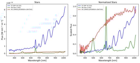
Figure 1.
The figures represent three different types of stars, (blue) symbiotic star [EM* AS 323], (red) red giant [2MASS J04390924+2847545], and (green) planetary nebula [Hen 2-442]. In the initial diagram, the flux values are denoted in Watts per nanometer per square meter (W/nm/m2), derived from external calibration using GaiaXpy library. In the adjacent figure, the flux values are normalized to a range between 0 and 1.
The normalization process allows for a clearer distinction between different types of spectra, even at a glance. The spectrum of the PN is predominantly composed of emission lines, while the RG spectra mainly exhibit a continuum with many absorption lines and/or bands. On the other hand, the SS spectra represent a combination of both, displaying emission lines and absorption bands in the IR region of the spectrum (700 to 1000 nm).
This dataset consists of 1975 records representing the spectra of the target stars. Each record is composed of 343 features, corresponding to the normalized flux values within the wavelength range of 336 to 1020 nm.
Furthermore, an extra column was incorporated in the dataset, which contains the corresponding labels for the star types. These labels are crucial for identifying and classifying each spectrum based on its category, enabling the utilization of supervised algorithms for training and prediction purposes.
The data exhibit a notable class imbalance, as there is a significant difference in the number of spectra for each star type. Data imbalance can have a detrimental impact on the performance of machine learning algorithms because they may struggle to learn patterns, and make inaccurate decisions for minority classes. This assertion was conclusively validated in Section 3.3, which further substantiates the analysis through weighted loss calculations and presents the outcomes of a ten-fold cross-validation procedure, assessing the findings by computing mean and standard deviation values.
To mitigate this issue and improve classification accuracy, data balancing techniques were implemented, such as oversampling the minority class and undersampling the majority class, ensuring an equitable distribution between both classes [15]. This approach allows classification algorithms to receive a balanced representation of the classes during training.
In addition to the data balancing techniques applied in this study, such as oversampling of minority classes and synthetic data generation with noise, it is important to consider other methods to address the imbalance. An alternative approach that can be effective is the use of weighted loss during model training. This technique assigns a higher weight to minority classes in the algorithm’s loss function, thus compensating for the disproportion in class representation without modifying the original dataset [16].
Our study will adopt a comparative approach, first analyzing the results obtained with the original imbalanced dataset and then comparing them with the outcomes after applying class balancing techniques. This methodology will allow us to objectively assess the impact of class imbalance on our specific problem and justify any decisions regarding the use of data balancing techniques.
The original dataset exhibits a significant imbalance in the representation of different star types, as illustrated in Table 2. This imbalance poses potential challenges for training machine learning algorithms, as it could lead to bias towards the majority class (red giant stars) and poor performance in classifying minority classes (symbiotic stars and planetary nebulae).
To address this issue, we propose a two-phase approach instead of immediately applying class balancing techniques:
- Initial analysis with imbalanced data—First, we will train and evaluate our models using the original imbalanced dataset. This will allow us to establish a baseline performance and assess the actual impact of class imbalance on our specific problem;
- Comparison with balanced data—If significant bias or poor performance is observed in the minority classes, we will proceed to apply class balancing techniques. We will use the oversampling method for minority classes, as described earlier, and compare the results with the original dataset.
As will be demonstrated in the following section, due to the class imbalance and the suboptimal performance exhibited by some algorithms on the imbalanced dataset, a decision was made to construct a balanced dataset. This new dataset ensures that each star type is represented by 1000 samples. The choice of selecting one thousand objects per class is based on several key factors. Firstly, this number is large enough to provide a representative and robust sample of each class, allowing machine learning algorithms to adequately capture the features and variability of the data. Additionally, having one thousand objects per class ensures a proper balance, mitigating bias toward the majority class and enhancing the model’s ability to generalize and correctly recognize objects from minority classes [17].
This balanced approach aims to address both the inherent class imbalance in the original data and the performance issues observed with certain algorithms (SVM and Naive Bayes), potentially leading to more accurate and reliable classification results across all star types. The comparative results of the algorithms’ performance on both the original imbalanced dataset and this new balanced dataset will be presented and discussed in detail in the Results section.
In the case of red giants, there was no issue, as the recovered quantity exceeded this number. Therefore, samples were randomly selected until the desired quantity was reached. However, in the case of symbiotic stars and planetary nebulae, the number of samples was insufficient. Therefore, the option was taken to generate new spectra from the original ones. To achieve this, the method of adding white noise was employed. A sequence of random numbers was generated, following a normal distribution with mean 0 and a variable standard deviation ranging from 0.01 to 0.05.
The process of generating new spectra involved combining the original data with the generated white noise (see Figure 2), and this allowed for an expansion of the dataset and a balancing of the classes, ensuring that all categories were adequately represented.
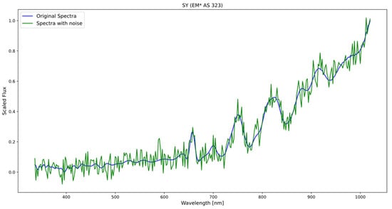
Figure 2.
The figure displays the original spectrum of the symbiotic star (blue) and the spectrum resulting from the addition of noise (green), following a normal distribution with a mean of 0 and a standard deviation of 0.05.
Applying the same level of standard deviation to all spectra, it is ensured that all samples have the same amount of added random variability. This avoids possible biases or excessive differences between the generated spectra, which could affect the interpretation and comparison of the results. These standard deviation values are in line with typical noise fluctuations observed in many scientific experiments and spectroscopic measurements.
This new balanced dataset, like the previous one, would consist of 343 features representing the flux values, and an additional column representing the spectrum label. In this case, a final count of 3000 spectra was achieved, with an equal distribution of 1000 spectra for each object type. This balanced dataset ensures that each type of star is adequately and proportionally represented, which is crucial to avoiding biases and enabling more accurate analysis and modeling. Table 3 presents the distribution of stellar spectra in the balanced dataset, categorized by star type. It illustrates the composition of each class, distinguishing between original spectra obtained from observations and those synthetically generated to achieve balance.
Table 3.
Class distribution in the balanced dataset, showing the proportion between original stellar spectra and synthetically generated ones for each star type.
2.3. Exploring Class Differences through t-SNE Visualization
To analyze potential differences between classes in our study, we employed the t-SNE (t-Distributed Stochastic Neighbor Embedding) algorithm. t-SNE is a popular unsupervised machine learning technique for data visualization and dimensionality reduction [18]. We applied t-SNE to our dataset, projecting it into lower dimensional spaces of two dimensions. By analyzing the resulting plots, we were able to identify clusters or groupings of samples that shared similar characteristics. These clusters provided insights into the presence of distinct classes and shed light on the differences between them. Additionally, t-SNE enabled the identification of outliers or samples that deviated from the main clusters.
The t-SNE projection of the balanced data shows a significant improvement in the separation and definition of class clusters. This indicates that the classes are more distinguishable from each other compared to the unbalanced data. The resulting visualization provides a clearer representation of the inherent differences between the classes (see Figure 3).
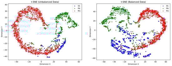
Figure 3.
t-SNE representation of unbalanced and balanced data in a two-dimensional space. The points represent samples from different classes. (Left) t-SNE projection of unbalanced data. A prominent cluster of the RG class is evident in the left side, whereas samples from the PN class are in the upper right region. The SS class exhibits weak clustering, blending with the other classes. (Right) t-SNE projection of balanced data in a two-dimensional space reveals improved separation and clustering of classes. The class clusters are more well-defined, although there still exist points that overlap with other classes.
However, despite this improvement, the presence of overlapping points between the classes can still be observed. This suggests that there may be inherent similarities or shared characteristics between certain samples from different classes. These areas of overlap indicate that the boundaries between the classes are not clearly defined and may represent cases where classification is more challenging.
It is important to note that, when applying machine learning algorithms to classify these classes, it is possible to achieve good overall results due to the improved separation and definition of the clusters, but it is also normal to expect some errors in classification due to the presence of overlapping points and similarities between the classes. However, it is expected that the performance will be improved (compared to t-SNE) since the number of parameters used is higher (in this case only the first two principal components are used).
2.4. Analysis and Selection of Algorithms
The formed datasets were divided into two subsets each. The first subset, representing 80% of the total samples, would be the training set, which was used to train various machine learning algorithms. This 80/20 split was chosen based on the Pareto principle or 80/20 rule, a common practice in machine learning. This division strikes a balance between having enough data to train robust models and retaining an adequate amount for subsequent validation [19]. During the training process, the algorithms learn patterns and relationships in the data to make predictions or decisions based on new data. The goal is for the algorithms to capture the underlying patterns in the training data and be able to generalize that knowledge to unseen data.
The other subset, representing the remaining 20%, was reserved for testing purposes. This dataset is used exclusively for evaluation and is not used during training. The aim of testing is to determine whether the algorithms have successfully learned and generalized without overfitting. Using a separate test set it helps detect if the algorithm has overfitted the training data, and provides a more realistic estimation of its performance.
For the analysis, the following supervised ML algorithms were used for classification: Random Forest, Support Vector Machine, Artificial Neural Networks, Gradient Boosting, and Naive Bayes. The selection of these algorithms provides a diverse combination of classification approaches, allowing for the evaluation and comparison of their performance on the test set. This enables us to obtain a more comprehensive understanding of their classification capability, and determine which one suits best our specific problem.
2.4.1. Algorithm Random Forest
Random Forest is a supervised machine learning algorithm that combines tree predictors in a way that each tree depends on the values of a randomly sampled vector, independently and with the same distribution for all trees in the forest [20]. Decision trees tend to overfit, meaning they learn the training data accurately but struggle to apply that knowledge to new data. However, it is possible to enhance their generalization ability by combining multiple trees into a set. This technique, known as an ensemble, has been proven to be highly effective in various problems, striking a balance between ease of use, flexibility, and the ability to apply learning to different situations.
An advantage of this algorithm is that it does not require scaled data. However, in our case, the data were normalized, which allows all parameters to have equal importance. Several training tests were conducted by varying the parameters provided to the algorithm in each case (See Table 4).
Table 4.
Description of the parameters used in the training of the Random Forest algorithm.
2.4.2. Algorithm Support Vector Machine
Support Vector Machine (SVM) is a supervised machine learning algorithm primarily used for data classification. Instead of directly operating on the original data, SVM represents them as points in a multi-dimensional space [21]. Each feature becomes a coordinate of these points, enabling us to visualize and analyze the relationships between variables. The goal of SVM is to find the hyper-plane that optimally separates the classes.
Different parameter tests were conducted, using different kernels for each one. Table 5 displays the analyzed configurations.
Table 5.
Description of the parameters used in training the SVM algorithm.
2.4.3. Algorithm Artificial Neural Networks
Artificial Neural Networks (ANN) are a subset of machine learning tools and are at the core of deep learning algorithms. Their name and structure are inspired by the human brain, trying to reproduce the way biological neurons send signals to each other. They consist of several layers of nodes, including an input layer, one or more hidden layers, and an output layer. ANNs possess high processing speeds and the ability to learn the solution to a problem from a set of examples [22].
The designed neural network has the following topology: an input layer of 64 neurons, followed by three hidden layers of 32 neurons each. All layers are dense, meaning all neurons are fully connected, and they use the ReLU activation function to introduce nonlinearity into the data. After each dense layer, a Dropout layer is added, which randomly deactivates 10% of the neurons during training. This helps prevent overfitting and improves the generalization ability of the model. The output layer consists of three neurons and uses the softmax activation function, commonly used in multiclass classification problems.
To compile the model, the “adam” optimizer is used, which is an optimization algorithm that adjusts the weights of the neural network during training. The loss function is set as “sparse_categorical_crossentropy”, which is suitable for multiclass classification problems with integer labels. Table 6 showcases the neural network configuration.
Table 6.
Description of the parameters used in training the ANN algorithm.
2.4.4. Algorithm Gradient Boosting
Gradient Boosting is an algorithm that focuses on numerical optimization of the function space rather than the parameter space. It is based on additive stage-wise expansions and aims to find an approximation of the objective function that minimizes a specific loss function. It works iteratively, where, at each stage, a new component is added to the existing approximation, adjusting it based on the gradient of the loss function. This allows for a gradual improvement of the approximation, and achieves competitive results in both regression and classification problems [23].
Different parameter combinations were tested, using various loss functions and different learning rates, among others, resulting in the following configurations (See Table 7).
Table 7.
Description of the parameters used in training the Gradient Boosting algorithm.
2.4.5. Algorithm Naive Bayes
The Naive Bayes classifier is a mathematical classification technique widely used in machine learning. It is based on Bayes’ Theorem and uses probabilistic calculations to find the most appropriate classification for a given dataset within a problem domain. It is very useful for cases where the number of target classifications is greater than two, making it more suitable for real-life classification applications [24] (see Table 8).
Table 8.
Description of the parameters used in the training of the Naive Bayes algorithm.
The algorithm was trained with the following configuration.
3. Results
3.1. Definition of Metrics
To compare the accuracy of the previously presented algorithms, the following metrics were used: Precision, F1-score, Recall (Sensitivity), and Cohen’s Kappa coefficient. These metrics were calculated after the algorithms evaluated the test dataset using the confusion matrix. This matrix displays the number of true positives (TP), true negatives (TN), false positives (FP), and false negatives (FN) for each class.
Precision is a metric that calculates the proportion of correct predictions in relation to the total number of samples [25]. It is useful for evaluating the overall performance of a classifier. The formula is as follows:
Recall is a metric that measures the proportion of positive instances that were correctly identified [25]. It is useful for evaluating the classifier’s ability to find all relevant samples of a specific class. The formula is as follows:
F1-score is a measure that combines Precision and Recall into a single value. It provides a balanced measure between the classifier’s precision and recall capabilities [25]. It is particularly useful when the dataset is imbalanced in terms of classes. The formula is as follows:
Cohen’s Kappa coefficient is a measure that expresses the level of agreement between two annotators in a classification problem [26]. It is defined as follows:
In our multiclass classification study, the evaluation metrics commonly used for binary classification problems were adapted for application in a multiclass context. To assess the performance of our classification model, we used the macro-averaged technique [27].
The choice of this approach was based on the need to treat all classes equally during evaluation, regardless of their size or data distribution. First, the metrics were calculated in a binary manner for each class individually, and then these metrics were averaged to obtain an overall evaluation of the model.
It is important to note that results from models trained on balanced and imbalanced datasets are not directly comparable due to differences in data distribution and model behavior. In addition to evaluating the performance, this study highlights how data balancing influences a model’s ability to generalize and accurately classify instances. By presenting the results separately, we aim to demonstrate the impact of data distribution on model performance and provide insights into the advantages and limitations of using balanced datasets.
3.2. Evaluation of Trained Models
3.2.1. Random Forest
Figure 4 displays the confusion matrix generated when running the Random Forest algorithm. It can be observed that the classification of symbiotic stars and planetary nebulae had higher imprecision. However, in the balanced dataset, despite the presence of errors, they are lower compared to the imbalanced dataset. This is reflected in the improved Recall value, which increased from 0.8575 to 0.9467, indicating a higher capability of the model to correctly identify stars. Table 9 presents the values obtained for all evaluated metrics using the Random Forest algorithm.
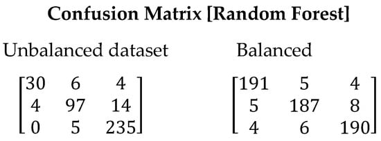
Figure 4.
Confusion matrix resulting from the execution of the Random Forest algorithm. On the left are the results with the unbalanced dataset and on the right with balanced dataset.
Table 9.
Metrics obtained from the Random Forest algorithm.
3.2.2. Support Vector Machine
The SVM algorithm exhibited poor performance in the tests conducted with the imbalanced dataset. In this scenario, the model tended to overfit and failed to generalize correctly, resulting in an incorrect classification of 12% of the total samples using the imbalanced dataset (See Figure 5). However, when using the balanced dataset, a significant improvement in performance was observed, with a considerable reduction in the classification error (6.16%). The recall value also improved from 0.7807 to 0.9383. Table 10 presents the values obtained for all evaluated metrics using the SVM algorithm.
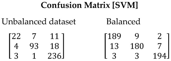
Figure 5.
Confusion matrix resulting from the execution of the SVM algorithm. On the left are the results derived with unbalanced dataset and on the right with balanced dataset.
Table 10.
Metrics obtained from the SVM algorithm.
3.2.3. Gradient Boosting
The Gradient Boosting algorithm has shown similar performance to Random Forest in our study. However, there is a presence of false positives due to the imbalance in the training data. Nevertheless, significant improvements are achieved when using the balanced dataset (See Figure 6). The F1-Score value increased from 0.8666 to 0.9283. This increase indicates a higher capability of the algorithm to correctly identify the relevant stars, thereby reducing false positives. Table 11 presents the values obtained for all evaluated metrics using the Gradient Boosting algorithm.
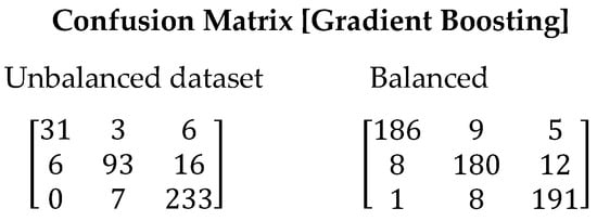
Figure 6.
Confusion matrix resulting from the execution of the Gradient Boosting algorithm. On the left are the results derived with the unbalanced dataset and on the right with the balanced dataset.
Table 11.
Metrics obtained from the Gradient Boosting algorithm.
3.2.4. Naive Bayes
The Naive Bayes algorithm achieved poor performance compared to other algorithms used in this study. One of the reasons for this low performance is its assumption of independence between features. This assumption may not hold true in many real-world cases, resulting in poor generalization and unsatisfactory results, as evidenced by the analysis of the confusion matrix in Figure 7. Even when conducting tests using balanced datasets, Naive Bayes fails to achieve adequate generalization compared to the previously used algorithms. This is reflected in lower F1-Score values, with 0.7877 for imbalanced data and 0.8005 for balanced data. Table 12 presents the values obtained for all evaluated metrics using the Gradient Boosting algorithm.
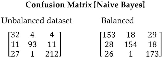
Figure 7.
Confusion matrix resulting from the execution of the Naive Bayes algorithm. On the left are the results derived with the unbalanced dataset and on the right with the balanced dataset.
Table 12.
Metrics obtained from the Naive Bayes algorithm.
3.2.5. Artificial Neural Networks
The Artificial Neural Networks algorithm showed superior results compared to the previous algorithms, achieving the highest overall precision values. This is evident in the confusion matrix shown in Figure 8, where a decrease in the number of false positives is observed for both the balanced and imbalanced datasets. The F1-Score value supports this claim, with a value of 0.9012 and 0.9533 for the imbalanced and balanced datasets, respectively (See Table 13). Its ability to capture complex relationships among the data and adapt to different patterns positions it as a favorable option, particularly in cases of imbalanced datasets.
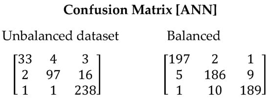
Figure 8.
Confusion matrix resulting from the execution of the ANN algorithm. On the left are the results derived with the unbalanced dataset and on the right with the balanced dataset.
Table 13.
Metrics obtained from the ANN algorithm.
3.3. Comparison of the Results
To comprehensively address class disparity, the models were evaluated using the imbalanced dataset with weighted loss, as illustrated in Table 14. This technique assigns different weights to minority and majority classes, allowing it to compensate for the imbalance and improve the model’s performance in predicting minority classes.
Table 14.
Comparison of the metrics obtained by the models on the unbalanced dataset with weighted loss.
Among the various algorithms evaluated, the Random Forest and Artificial Neural Networks stood out as the top performers in handling the class imbalance issue. These two algorithms exhibited remarkable performance, achieving precision values of 0.9467 and 0.9532, respectively, when trained on the balanced dataset. Even with the imbalanced dataset, their performance remained robust—Random Forest achieved a precision of 0.9031, while the Neural Network reached 0.9312. These findings demonstrate the superior effectiveness of these two algorithms in handling imbalanced data compared to other approaches.
Table 15 and Table 16 provide a comprehensive comparison of the metrics obtained using balanced and imbalanced data, respectively. These two standout algorithms will be utilized to validate new spectra candidates for symbiotic stars and planetary nebulae classification in the next section.
Table 15.
Comparison of the metrics obtained by the models on the unbalanced dataset.
Table 16.
Comparison of the metrics obtained by the models on the balanced dataset.
Given their outstanding performance, the Random Forest and Artificial Neural Networks models were selected for further validation using a rigorous ten-fold cross-validation approach. This validation was applied exclusively to the balanced dataset, which was augmented with synthetic noise using oversampling techniques. To ensure the robustness of the evaluation process, care was taken to prevent any overlap between original records and their artificial counterparts across different folds. Following best practices for handling artificial records, if an original record was included in the training set of a given fold, its noisy artificial versions were excluded from the test set of the same fold. To meet this requirement, the original and generated spectra were kept within the same fold. This strategy prevented any overlap between original records and their artificial counterparts during evaluation. The results of this evaluation are summarized in Table 17 and Table 18.
Table 17.
Validation metrics (average and standard deviation) for Artificial Neural Networks using ten-fold cross-validation on the balanced dataset.
Table 18.
Validation metrics (average and standard deviation) for Random Forest using ten-fold cross-validation on the balanced dataset.
The results obtained through 10-fold cross-validation on the balanced dataset were notable, with mean precision values of 0.92086 for Random Forest and 0.9235 for Artificial Neural Networks. Despite mitigating the potential bias associated with the addition of synthetic data, the results were satisfactory, slightly surpassing those achieved with the imbalanced dataset.
3.4. Second Evaluation of Trained Models
3.4.1. Suspected Symbiotic Stars
To assess the effectiveness and demonstrate the practical application of the trained models, we conducted the classification of two sets of stars suspected to be symbiotic stars. For this task, we utilized the ANN and Random Forest models, which showed superior performance in the earlier tests.
The first dataset used was obtained from the article “A catalogue of symbiotic stars” [28], initially consisting of 30 candidate symbiotic stars. From the original dataset, common stars used in the model training process were excluded, as well as those lacking spectral information in GDR3. The result of this careful selection process was a set of 15 stars, which were subsequently evaluated using our previously trained models, as detailed in Table 19. The Figure 9 shows the spectral representation of the stars obtained previously from the article.
Table 19.
Results of the classification using ANN and Random Forest. Both algorithms were trained using both balanced and imbalanced datasets. The dataset of suspected symbiotic stars was obtained from the article “A catalogue of symbiotic stars” [28]. The ANN model’s results are expressed as probabilities with four significant digits, whereas the Random Forest model only shows the resulting class.
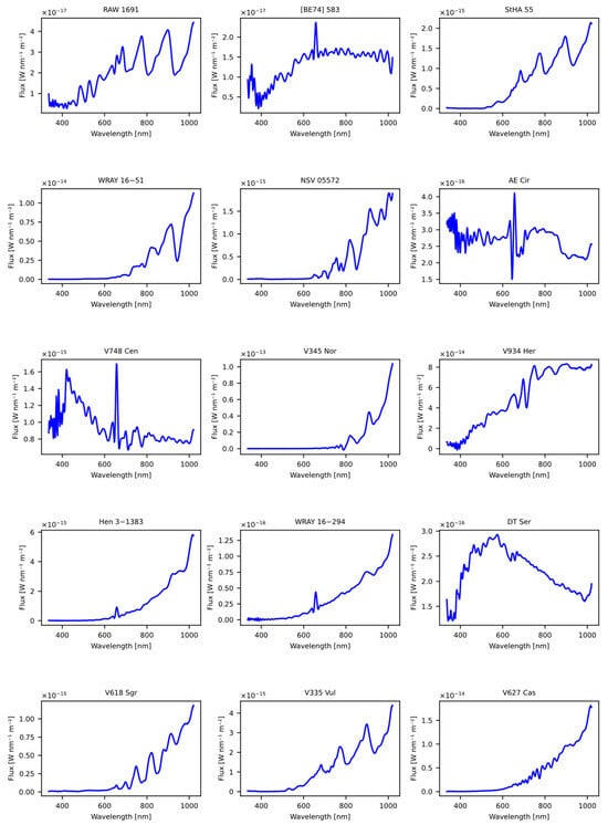
Figure 9.
The figure displays the spectra obtained from the Gaia DR3 catalog that were sourced from the article “A catalogue of symbiotic stars” [28].
The second dataset was obtained from the article “A machine learning approach for identification and classification of symbiotic stars using 2MASS and WISE” [20]. Like the dataset obtained from the previous article, common stars used to train the models were removed, as well as those lacking spectral information in GDR3. The outcome of this selection process was a set of 17 stars, which were subsequently evaluated using the previously trained models, as detailed in Table 20. The Figure 10 shows the spectral representation of the stars obtained previously from the article.
Table 20.
Results of the classification using ANN and Random Forest. Both algorithms were trained using both balanced and imbalanced datasets. The dataset of suspected symbiotic stars was obtained from the article “A machine learning approach for identification and classification of symbiotic stars using 2MASS and WISE” [29]. The ANN model’s results are expressed as probabilities with four significant digits, whereas the Random Forest model only shows the resulting class.
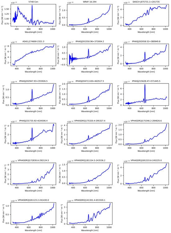
Figure 10.
The figure displays the spectra obtained from the Gaia DR3 catalog that were sourced from the article “A machine learning approach for identification and classification of symbiotic stars using 2MASS and WISE” [29].
The use of spectral information in the training of the models allowed for capturing specific characteristics and patterns associated with symbiotic stars. Spectral properties, such as emission and absorption lines, played a crucial role in the classification of the stars.
However, the quality and reliability of the obtained results must be analyzed with caution. Although most of the stars were classified as symbiotic by the models, further validation is necessary to effectively confirm the true nature of the classified stars. To achieve this, new models trained with the whole spectra could be employed.
Furthermore, it is important to consider other types of stars to increase the size of the dataset and achieve the better generalization of the models.
3.4.2. Suspected Planetary Nebulae
In addition to the previous tests, an additional analysis was conducted using a carefully selected set of 15 stars that are considered candidates for planetary nebulae. Following this careful selection process, this group of stars was evaluated using our previously trained models, as detailed in Table 21. This information was obtained from the Symbad database.
Table 21.
Results of the classification using ANN and Random Forest. Both algorithms were trained using both balanced and imbalanced datasets. The dataset of suspected planetary nebulae stars was obtained from the Symbad online database. The ANN model’s results are expressed as probabilities with four significant digits, whereas the Random Forest model only shows the resulting class.
The purpose of including this group of 15 candidate stars for planetary nebulae in the study was to further expand the understanding of the models and their ability to identify and classify specific celestial objects. The Figure 11 shows the spectral representation of the stars obtained previously from the article.
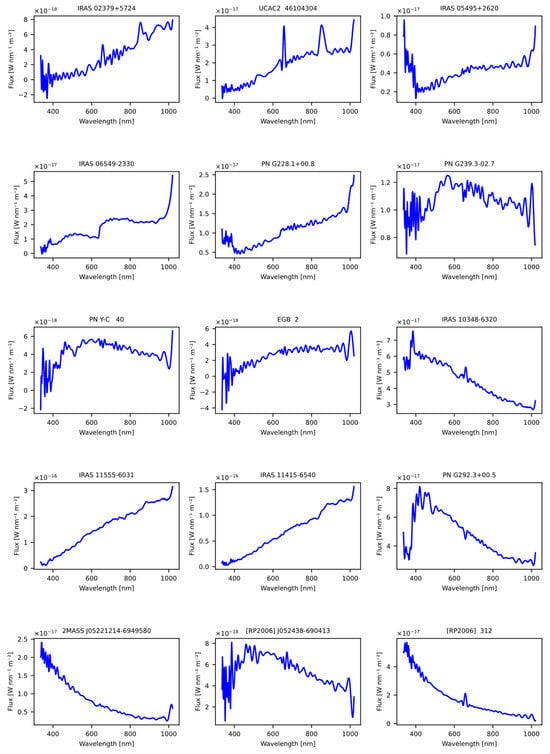
Figure 11.
The figure displays the spectra of suspected planetary nebulae stars obtained from the Gaia DR3 catalog that were sourced from Symbad database online.
4. Discussion
This study focuses on the classification of symbiotic stars, planetary nebulae, and red giants using machine learning techniques, contributing to the growing application of artificial intelligence in astronomy. Unlike previous works centered on more general classifications, this specific approach represents a significant advancement in the classification of stellar objects in advanced evolutionary stages. The results obtained with Random Forest and Artificial Neural Networks surpass previous studies, such as that of Kheirdastan and Bazarghan [30], achieving accuracies above 90% in both balanced and unbalanced datasets, compared to the previously reported 80%.
A distinctive aspect of this work is the explicit approach to the problem of class imbalance, a common challenge relating to real astronomical data. While Qi used the SMOTE technique to handle imbalance [31], our study directly compares the performances of models on balanced and unbalanced sets, providing valuable insights into the robustness of algorithms under realistic conditions. The effectiveness demonstrated by Artificial Neural Networks, especially with unbalanced data, aligns with recent trends, such as that shown in the work of Zhao Z. on the classification of stellar spectra [32].
Despite the significant achievements, limitations similar to those mentioned by Tamez Villarreal and Barton are acknowledged in terms of the diversity and size of the datasets used. It is suggested that future studies focus on expanding the database, including a greater variety of objects and observational conditions [33], so as to further improve the robustness and generalization of the models.
5. Conclusions
The study focused on the classification of the following astronomical objects: symbiotic stars, planetary nebulae, and red giants. It was observed that red giants were more numerous and represented a larger proportion compared to the other classes. This imbalance caused difficulties in classification, as the models tended to confuse part of the minority classes (symbiotic stars and planetary nebulae) with the majority class (red giants).
It was found that the Random Forest and ANN algorithms showed satisfactory results, with accuracy values of 0.9467 and 0.9532, respectively, for the balanced dataset. On the other hand, for the imbalanced dataset, Random Forest achieved an accuracy of 0.9031, while the ANN achieved an accuracy of 0.9312. Therefore, these algorithms demonstrate greater effectiveness on imbalanced datasets compared to other approaches. ANN proved to be highly effective when working with imbalanced datasets due to their ability to learn complex patterns and adapt to different class distributions.
As a result of our research, two machine learning models were successfully trained to classify peculiar stars with high accuracy. These models have been validated using diverse datasets, demonstrating their effectiveness in real-world scenarios. Additionally, these models can be employed to classify stars that are difficult to categorize, including those without prior classification or those considered potential candidates for peculiar stars. This functionality enhances their effectiveness in identifying and assessing previously ambiguous or uncertain stellar objects.
These classification models present a valuable and highly useful tool for astronomers, providing effective support in the classification of peculiar stars. Their application significantly contributes to a better understanding of the stellar life cycle.
Author Contributions
Data Curation, O.J.P.C.; Formal analysis, O.J.P.C.; Conceptualization, C.A.M.P., S.G.N.J., L.J.C.E. and M.M.O.; Methodology, C.A.M.P., S.G.N.J. and L.J.C.E.; Software, O.J.P.C.; Validation, S.G.N.J. and O.J.P.C.; Visualization, O.J.P.C.; Investigation, O.J.P.C., C.A.M.P. and S.G.N.J.; Resources, C.A.M.P. and M.M.O.; Writing—original draft, O.J.P.C.; Writing—review & editing, C.A.M.P., S.G.N.J., L.J.C.E. and M.M.O.; Supervision, C.A.M.P., S.G.N.J., L.J.C.E. and M.M.O. All authors have read and agreed to the published version of the manuscript.
Funding
This research received no external funding.
Institutional Review Board Statement
Not applicable.
Informed Consent Statement
Not applicable.
Data Availability Statement
All original contributions and findings presented in this study are documented within the article. The data supporting the results, along with the tests conducted and the corresponding code, are available in the publicly accessible GitHub repository: https://github.com/opcruz/gaiaDR3ML (accessed on 29 July 2024). Should additional details or clarifications be required, further inquiries can be directed to the corresponding author.
Acknowledgments
We would like to acknowledge the use of artificial intelligence, specifically ChatGPT 3.5, in the preparation of this article. AI was utilized to assist us in improving the clarity and readability of certain paragraphs, ensuring the language was more accessible. Additionally, AI supported us in translating specific sections into English to maintain accuracy. However, we would like to emphasize that AI was not used to generate any new information or content; it solely served as a tool to refine the presentation of the material we had already developed. All original research, analysis, and conclusions presented in this article are the work of the authors.
Conflicts of Interest
The authors declare no conflict of interest.
References
- Prusti, T.; de Bruijne, J.H.J.; Vallenari, A.; Babusiaux, C.; Bailer-Jones, C.A.L.; Bastian, U.; Biermann, M.; Evans, D.W.; Eyer, L.; Gaia Collaboration; et al. The Gaia mission. Astron. Astrophys. 2016, 595, A1. [Google Scholar] [CrossRef]
- Witten, C.E.C.; Aguado, D.S.; Sanders, J.L.; Belokurov, V.; Evans, N.W.; Koposov, S.E.; Prieto, C.A.; De Angeli, F.; Irwin, M.J. Information content of BP/RP spectra in Gaia DR3. Mon. Not. R. Astron. Soc. 2022, 516, 3254–3265. [Google Scholar] [CrossRef]
- Babusiaux, C.; Fabricius, C.; Khanna, S.; Muraveva, T.; Reylé, C.; Spoto, F.; Vallenari, A. Gaia Data Release 3—Catalogue validation. Astron. Astrophys. 2023, 674, A32. [Google Scholar] [CrossRef]
- Carrasco, J.M.; Weiler, M.; Jordi, C.; Fabricius, C.; De Angeli, F.; Evans, D.W.; van Leeuwen, F.; Riello, M.; Montegriffo, P. Internal calibration of Gaia BP/RP low-resolution spectra. Astron. Astrophys. 2021, 652, A86. [Google Scholar] [CrossRef]
- Gaia Data Release 3 Contents Summary—Gaia-Cosmos. Available online: https://www.cosmos.esa.int/web/gaia/dr3 (accessed on 23 November 2022).
- Karttunen, H.; Kröger, P.; Oja, H.; Poutanen, M.; Donner, K.J. Fundamental Astronomy; Springer: Berlin/Heidelberg, Germany, 2017. [Google Scholar] [CrossRef]
- Jastrow, R. Red Giants and White Dwarfs; W. W. Norton & Company: New York, NY, USA, 1990; p. 269. [Google Scholar]
- Frankowski, A.; Soker, N. Very late thermal pulses influenced by accretion in planetary nebulae. New Astron. 2009, 14, 654–658. [Google Scholar] [CrossRef]
- Kwok, S. The Origin and Evolution of Planetary Nebulae; Cambridge University Press: New York, NY, USA, 2000; Volume 243. [Google Scholar]
- Mikolajewska, J. Symbiotic stars: Observations confront theory. arXiv 2012, arXiv:1110.2361. [Google Scholar] [CrossRef]
- Carroll, B.W.; Ostlie, D.A. An Introduction to Modern Astrophysics, 2nd ed.; Cambridge University Press (CUP): Cambridge, UK, 2019; pp. 1–1341. [Google Scholar] [CrossRef]
- Gaia Collaboration; Vallenari, A.; Brown, A.; Prusti, T. Gaia Data Release 3: Summary of the content and survey properties. Astron. Astrophys. 2022, 674, A1. [Google Scholar] [CrossRef]
- Wenger, M.; Ochsenbein, F.; Egret, D.; Dubois, P.; Bonnarel, F.; Borde, S.; Genova, F.; Jasniewicz, G.; Laloë, S.; Lesteven, S.; et al. The SIMBAD astronomical database—The CDS reference database for astronomical objects. Astron. Astrophys. Suppl. Ser. 2000, 143, 9–22. [Google Scholar] [CrossRef]
- Gopal, S.; Patro, K.; Sahu, K.K. Normalization: A Preprocessing Stage. Int. Adv. Res. J. Sci. Eng. Technol. 2015, 2, 20–22. [Google Scholar] [CrossRef]
- Tyagi, S.; Mittal, S. Sampling Approaches for Imbalanced Data Classification Problem in Machine Learning. In Lecture Notes in Electrical Engineering; Springer: Cham, Switzerland, 2020; Volume 597, pp. 209–221. [Google Scholar] [CrossRef]
- Fernando, K.R.M.; Tsokos, C.P. Dynamically Weighted Balanced Loss: Class Imbalanced Learning and Confidence Calibration of Deep Neural Networks. IEEE Trans. Neural Netw. Learn. Syst. 2022, 33, 2940–2951. [Google Scholar] [CrossRef]
- Rahman, M.M. Sample Size Determination for Survey Research and Non-Probability Sampling Techniques: A Review and Set of Recommendations. J. Entrep. Bus. Econ. 2023, 11, 42–62. [Google Scholar]
- Van Der Maaten, L.; Hinton, G. Visualizing data using t-SNE. J. Mach. Learn. Res. 2008, 9, 2579–2605. [Google Scholar]
- Vrigazova, B. The Proportion for Splitting Data into Training and Test Set for the Bootstrap in Classification Problems. Bus. Syst. Res. Int. J. Soc. Adv. Innov. Res. Econ. 2021, 12, 228–242. [Google Scholar] [CrossRef]
- Breiman, L. Random Forests. Mach. Learn. 2001, 45, 5–32. [Google Scholar] [CrossRef]
- Noble, W.S. What is a support vector machine? Nat. Biotechnol. 2006, 24, 1565–1567. [Google Scholar] [CrossRef]
- Bishop, C.M. Neural networks and their applications. Rev. Sci. Instrum. 1998, 65, 1803. [Google Scholar] [CrossRef]
- Friedman, J.H. Greedy function approximation: A gradient boosting machine. Ann. Stat. 2001, 29, 1189–1232. [Google Scholar] [CrossRef]
- Yang, F.J. An implementation of naive bayes classifier. In Proceedings of the 2018 International Conference on Computational Science and Computational Intelligence, CSCI, Las Vegas, NV, USA, 12–14 December 2018; pp. 301–306. [Google Scholar] [CrossRef]
- Powers, D.M.W. Evaluation: From precision, recall and F-measure to ROC, informedness, markedness and correlation. arXiv 2020, arXiv:2010.16061. [Google Scholar]
- Chicco, D.; Warrens, M.J.; Jurman, G. The Matthews Correlation Coefficient (MCC) is More Informative Than Cohen’s Kappa and Brier Score in Binary Classification Assessment. IEEE Access 2021, 9, 78368–78381. [Google Scholar] [CrossRef]
- Farhadpour, S.; Warner, T.A.; Maxwell, A.E. Selecting and Interpreting Multiclass Loss and Accuracy Assessment Metrics for Classifications with Class Imbalance: Guidance and Best Practices. Remote Sens. 2024, 16, 533. [Google Scholar] [CrossRef]
- Belczyński, K.; Mikołajewska, J.; Munari, U.; Ivison, R.J.; Friedjung, M. A catalogue of symbiotic stars. Astron. Astrophys. Suppl. Ser. 2000, 146, 407–435. [Google Scholar] [CrossRef]
- Akras, S.; Leal-Ferreira, M.L.; Guzman-Ramirez, L.; Ramos-Larios, G. A machine learning approach for identification and classification of symbiotic stars using 2MASS and WISE. Mon. Not. R. Astron. Soc. 2019, 483, 5077–5104. [Google Scholar] [CrossRef]
- Kheirdastan, S.; Bazarghan, M. SDSS-DR12 bulk stellar spectral classification: Artificial neural networks approach. Astrophys. Space Sci. 2016, 361, 304. [Google Scholar] [CrossRef][Green Version]
- Qi, Z. Stellar Classification by Machine Learning. SHS Web Conf. 2022, 144, 03006. [Google Scholar] [CrossRef]
- Zhao, Z.; Wei, J.; Jiang, B. Automated Stellar Spectra Classification with Ensemble Convolutional Neural Network. Adv. Astron. 2022, 2022, 4489359. [Google Scholar] [CrossRef]
- Villarreal, J.T.; Barton, S. Stellar Classification based on Various Star Characteristics using Machine Learning Algorithms. J. Stud. Res. 2023, 12. [Google Scholar] [CrossRef]


Disclaimer/Publisher’s Note: The statements, opinions and data contained in all publications are solely those of the individual author(s) and contributor(s) and not of MDPI and/or the editor(s). MDPI and/or the editor(s) disclaim responsibility for any injury to people or property resulting from any ideas, methods, instructions or products referred to in the content. |
© 2024 by the authors. Licensee MDPI, Basel, Switzerland. This article is an open access article distributed under the terms and conditions of the Creative Commons Attribution (CC BY) license (https://creativecommons.org/licenses/by/4.0/).