Climate Change and Building Renovation: The Impact of Historical, Current, and Future Climatic Files on a School in Central Italy

Abstract

Climate change significantly affects the operating environment of buildings. These changes impact both energy efficiency and occupants’ comfort and remain crucial even in building restoration, where design decisions typically rely on historical data, yet performance depends on anticipated future scenarios. The present work evaluates the impact of different climate datasets on dynamic energy simulations for an educational building in Central Italy, focusing on estimating heating demands across historical, current, and future climatic scenarios. The assessment considers both the building’s current state and potential energy-efficient retrofits. Initially, various meteorological datasets, including measured and model-generated data, are selected to predict key weather parameters. The analysis reveals the potential and limitations of regional climate models (RCMs) in estimating these variables, with the MM5 dataset emerging as the most reliable. Subsequently, the energy performance of the reference building and its vulnerability to climate change are assessed. Our results show significant differences in energy demand based on construction periods, with the oldest section consuming 29% to 54% more energy monthly than the newer sections. Moreover, using non-representative climatic files can lead to prediction errors of up to 199%. Finally, the building’s energy behaviour is analysed under future climate conditions by generating typical meteorological years (TMYs) for 2030, 2050, and 2070. This analysis evaluates the energy requirements for both existing and retrofitted building configurations. The findings confirm that retrofit interventions with high-performance insulation and upgraded windows significantly enhance the building’s energy efficiency and resilience to future climate conditions, leading to annual energy savings of 50% to 57%.

1. Introduction

The household sector is one of the main contributors to energy use and greenhouse gas (GHG) emissions and impacts more than the industry, transportation, and land use for agricultural purposes [1]. According to the 2020 annual report from the World Green Building Council (WorldGBC), global carbon emissions related to building operations surged from 19% in 2010 to 28% in 2020. Concurrently, building energy consumption grew from 32% to 36% during the same period [2]. Notably, heating, ventilation, and air-conditioning (HVAC) systems, responsible for nearly 70% of the total energy demand, impose the greatest energy requirements.

Key factors influencing building thermal loads and vulnerability to climate change are weather conditions and construction age. Tropical climates, for example, have to face the continuous increase in summer energy demand more than other locations, and deeper impacts are experienced by older buildings not designed with advanced technologies such as energy-efficient equipment or adequate insulation [3,4,5]. Beyond environmental concerns, economic implications also matter. Clarke et al. [6] projected significant expenditure increases in low-latitude countries, which currently have minimal heating needs but anticipate higher cooling demands.

Zhu et al. [7] identified two main approaches for estimating building energy needs under future climates: direct predictions based on statistical analyses and indirect projections through building simulation tools. Several studies focus on understanding the impact of varying climatic parameters on global building energy loads. These investigations reveal higher cooling demands and reduced heating requirements compared to historical and current data [8,9,10,11,12,13,14,15,16].

For instance, Berardi and Jafarpur [17] predicted a 15–126% increase in cooling energy and an 18–33% decrease in heating by 2070. Similarly, Cellura et al. [18] estimated 50–119.7% higher yearly heating and cooling needs in Southern Europe by 2090. In addition to the increase in building energy needs, considerations about comfort conditions become essential, especially for the summer period when air conditioning aids natural ventilation, if present, and prevents discomfort [19].

To mitigate building energy demands due to global warming and ensure comfort, adopting energy-efficient measures like advanced building envelopes and sustainable cooling strategies is essential [20,21,22,23,24]. Implementing climate-responsive retrofit solutions, in fact, can reduce total building energy use by 54–58% under current and future scenarios [25].

In the context of building energy renovation, a crucial aspect is the retrofitting of school buildings. This is particularly important given that approximately 90% of educational buildings are over 30 years old and must meet European performance standards [26]. Moreover, creating a database of energy consumption for such buildings under varying climates is crucial, especially for experimental campaigns, considering peak energy needs during specific periods [27].

Santamaouris et al. [28] demonstrated that energy conservation strategies can lower school energy consumption by 20%. Among the retrofit solutions evaluated by researchers all over the world, the most adopted involve novel technologies for both inner and outer envelopes [29]. Examples include improving energy performance by enhancing insulation and replacing low-quality windows [30]. Investigations like Rospi et al. [31] also explore replacing existing systems with heat pumps, yielding 40–60% energy savings, potentially rising to 75–90% with equipment and envelope upgrades.

In addition to the poor energy performances generally associated with educational buildings, considerations about indoor comfort and air quality conditions become crucial. In recent decades, there has been a focus on indoor environmental quality (IEQ) in schools due to its impact on student and teacher health and productivity [32,33,34,35]. Tucker and Izadpanahi’s study [36] highlights schools’ role in promoting environmental attitudes among students. Buildings designed or adapted sustainably have a positive impact, fostering greater sensitivity to environmental issues among attending students.

Based on these main findings, the present work aims to evaluate the energy performance of an educational building under historical, current, and future climate conditions, considering both its current state and potential improvements. In general, the importance of using accurate climate data for dynamic simulations is undervalued. The common tendency is to adopt outdated weather data that no longer represent the specific location. Additionally, many studies evaluate energy retrofit solutions without properly accounting for future climate conditions, leading to inaccurate results. Thus, the collection and generation of high-quality weather data play a pivotal role in accurately describing the real energy behaviour of buildings, as demonstrated in previous work [37].

Finally, the case study chosen for this research is particularly significant, not only because it represents the typical characteristics of the Italian educational building stock but also because it was erected in different periods, showcasing a range of construction techniques. This diversity provides a unique opportunity to comprehensively evaluate the building’s energy performance. By analysing this structure, the study offers valuable insights into the broader context of Italian educational buildings, providing data that can guide future upgrades and inform policy decisions at a national level.

The paper is structured as follows: after this introduction, climate change considerations on both global and local scales are reported in Section 2. Section 3 and Section 4 synthesise the methodology and weather sources adopted for generating or collecting real and measured data. Section 5 describes the case study and its input parameters for the building’s dynamic energy simulations and validation. Then, the obtained results are shown and described in Section 6. Finally, Section 7 draws the main conclusions.

2. The Climate Change Scenario

In recent decades, scientists worldwide have expressed significant concerns regarding climate change and global warming. The Intergovernmental Panel on Climate Change (IPCC), a United Nations body responsible for assessing climate science, stands as one of the pioneering organisations in this field. According to the IPCC’s Sixth Assessment Report, the projected climate response to GHG emissions scenarios suggests a likely warming range for the period 2081–2100. This range varies from 1.4 °C for a scenario with very low GHG emissions to 2.7 °C for an intermediate emissions scenario and up to 4.4 °C for a scenario with very high GHG emissions [38]. Additionally, predictions indicate that annual greenhouse gas emissions between 2011 and 2020 are set to exceed those of any previous decade [39]. These estimations underscore the urgency of addressing climate change, which has both short-term impacts, such as severe weather events like storms, floods, and landslides, and long-term effects, which involve gradual changes in weather patterns as temperature variations, solar radiation increases, and rising sea levels [40].

The IPCC’s recognition of climate change as a pressing global issue has led to the development of various climate scenarios aimed at predicting weather variations. Over time, these scenarios have been updated to incorporate changes in political developments, protocols, and international agreements related to the sector. The two most recent sets of scenarios introduced by the IPCC are the Special Report on Emissions Scenarios (SRES) and the Representative Concentration Pathways (RCPs). These scenarios encompass a range of radiative forcing levels examined in scientific literature and provide essential input for climate model simulations. It is important to note that these scenarios focus on consistent projections of radiative forcing components, using concentrations as the primary output of RCPs, which are designed as inputs for climate models. This framework has been predicted to yield four pathways with radiative forcing levels of 8.5, 6.0, 4.5, and 2.6 W/m² by the century’s end, covering the period from 1850 to 2100 [41,42].

Europe is experiencing a faster rate of warming than the global average, leading to persistent environmental, societal, and economic challenges. The mean annual temperature has risen by up to 2.19 °C compared to the pre-industrial period, with particularly pronounced warming in Eastern Europe, Scandinavia, and the Eastern part of the Iberian Peninsula [43]. Studies also predict increased frequency, duration, and severity of meteorological and hydrological droughts across most European countries throughout the 21st century [44].

Turning our attention to the Italian Peninsula, climate change predictions suggest an average temperature increase of 1.8–3.1 °C under the RCP4.5 scenario and 3.5–5.4 °C under the RCP8.5 scenario over the span of a century [45]. In addition, more substantial temperature rises are foreseen during the summer season, with average increments of 2.5–3.6 °C and 4.2–7.0 °C for the RCP4.5 and RCP8.5 scenarios, respectively. These temperature changes, alongside broader climate shifts, impact indoor environments and building requirements, resulting in heightened energy demand for HVAC systems.

In an era defined by the pressing challenge of climate change, evaluating building retrofit solutions with a keen eye on estimating future climatic conditions has become of paramount importance. By thoroughly assessing restorative measures in the context of changing climate patterns, buildings are not only energy-efficient but also resilient to intensifying environmental conditions. Within this framework, the present work focuses not solely towards the energy performance of the selected reference building within historical and contemporary climate conditions but also intends to appraise the enhancements attainable through the implementation of the analysed retrofit options while considering future climate projections.

3. Materials and Methods

The work developed in the present investigation is summarised in Figure 1, and the adopted methodology is described in the following subsections.

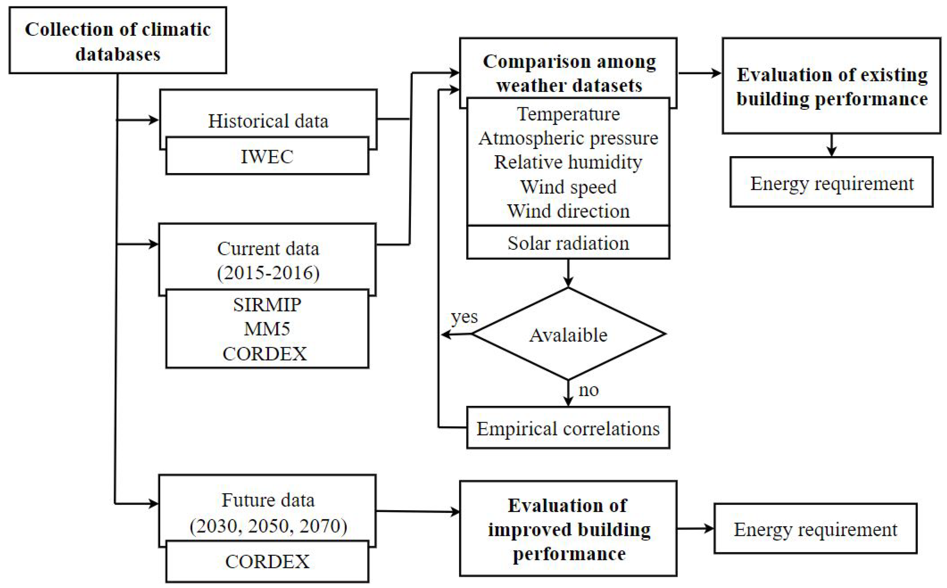
3.1. Collection and Comparisons of Climate Files

In the first stage of this paper, various weather datasets are selected and collected or predicted from real or virtual weather stations. Specifically, the International Weather for Energy Calculation (IWEC), derived from an experimental campaign spanning from 1951 to 1970, is assumed as the historical typical meteorological year (TMY). Additionally, climatic parameters measured during 2015–2016 are gathered for Ancona, and simultaneously, the Fifth Mesoscale Model (MM5) and the COordinated Regional Downscaling Experiment (CORDEX) are adopted to generate a database covering the same period. Furthermore, CORDEX is also used to estimate future TMYs for both near and distant futures.

These climatic parameters encompass essential variables for conducting dynamic energy simulations, including air temperature, atmospheric pressure, relative humidity, wind speed and direction, and global solar radiation. In addition, the current section also focuses on estimating solar radiation without direct measurements using empirical correlations. In detail, the calculation of the solar components is approached through two methods: the first employs the Campbell and Norman algorithm [46], while the second utilises the correlation specific to the Mediterranean region in the Northern Hemisphere [47]. Both methods are better described in Section 4.

The investigated databases are compared employing Taylor diagrams [48] to evaluate the differences estimated for the selected sources on both seasonal and annual scales. This method provides key statistics like the correlation coefficient, the root-mean-square value, and standard deviation with respect to a reference pattern.

Naming f the pattern assumed as reference quantity (i.e., the temperature or the global radiation) and r the pattern of another climatic file, the correlation coefficient (R) and the centred root-mean-square difference ($RMSD$) are evaluated, respectively, through Equations (1) and (2). To facilitate comparison, the RMSD and standard deviation (${\sigma }_r$) values are then normalised by dividing these quantities by the standard deviation of the corresponding observed value.

$$R={\displaystyle \frac{\frac{1}{N}{\displaystyle \sum _{n=1}^N}\left(f_n-\overline{f}\right)\left(r_n-\overline{r}\right)}{{\sigma }_f·{\sigma }_r}},$$

(1)

$$RMSD={\displaystyle \frac{1}{N}}\sum _{n=1}^N{\left[\left(f_n-\overline{f}\right)-\left(r_n-\overline{r}\right)\right]}^2,$$

(2)

$${\sigma }_f^2={\displaystyle \frac{1}{N}}\sum _{n=1}^N{\left(f_n-\overline{f}\right)}^2,$$

(3)

$${\sigma }_n^2={\displaystyle \frac{1}{N}}\sum _{n=1}^N{\left(r_n-\overline{r}\right)}^2.$$

(4)

3.2. Energy Performance Assessment of a Building in Central Italy under Historical and Current Climate Conditions

The second stage assesses the influence of these databases on building energy requirements. To quantify the impact of climate files on the outcomes, a school in Ancona, representative of the existing educational building stock, is selected for dynamic simulations. These simulations are conducted following a preliminary validation phase based on energy consumption data, which is extrapolated from utility bills collected over the analysed years (September 2015–August 2016).

Energy simulations are performed using DesignBuilder software (version 6), and the case study is meticulously modelled to better represent its actual energy performance.

3.3. Climate Change and Retrofit Solutions

The final step involves generating and applying future climate data to assess the impact of climate change on the case study, both in its current form and in an energy-efficient retrofitted version. Specifically, the two retrofit solutions considered here include adding an insulation layer made of either glass wool or expanded polystyrene (EPS) to improve the building’s thermal performance. Additionally, the inefficient glazed surfaces are replaced with more energy-efficient alternatives.

The building’s projected energy consumption is then estimated for typical meteorological years representing the conditions in 2030, 2050, and 2070, and comparisons are made between the current and improved configurations.

4. Weather Data Sources

The selected case study consists of an educational building located in Ancona, a coastal city in Central Italy, positioned at 43°37′ N latitude and 13°31′ E longitude. Ancona is 110 m above sea level and has a typical Mediterranean climate. This climate is characterised by dry, hot summers and mild winters, falling under the “Cfa” Köppen–Geiger climate classification [49]. In this classification, “C” indicates warm temperature climates, “f” signifies full humidity without a dry season, and “a” represents a hot summer.

According to EN ISO 13790:2004 [50] and the references within the Italian energy code [51], the site falls into climate zone “D”. This zone has an external winter design temperature of −2 °C and 1688 degree days. Ancona experiences an average annual temperature of 14.4 °C. The warm season spans from June to mid-September, featuring average high temperatures of 29 °C and lows of 19 °C. The cold season, lasting from November to March, sees temperatures mostly below 12 °C.

For this study, a variety of sources contribute to different climatic datasets used for analysis. Observed meteorological data are collected from an Ancona weather station. These observations are compared with simulated values derived from different regional climate models and the averaged IWEC database. Additionally, projections of future weather conditions are calculated to assess the potential impact of climate change on buildings. This information guides the development of more energy-efficient retrofit solutions.

4.1. Observed Meteorological Data

The first climatic file is sourced from real observations acquired by the meteo-mast situated on the roof of the Marche Region building and belonging to the SIRMIP meteorological network. These data span the years 2015 and 2016, coinciding with the available information on building energy consumption. The data are recorded at 30 min intervals, which are then consolidated into hourly intervals to facilitate comparisons with the EnergyPlus climatic data. The meteo-tower is equipped with sensors able to measure various parameters, including global solar radiation, air temperature, relative humidity, ambient pressure, wind speed, and wind directions.

The measured global radiation is subdivided into direct and diffuse components, as the DesignBuilder software necessitates. For this reason, the Campbell and Norman algorithm and empirical correlations are adopted.

The Campbell and Norman method calculates the possibility of obtaining the ratio between direct and diffuse components at each time step. These percentage values are then applied to the corresponding experimental measurements of global radiation. In detail, this model relies on input data such as recorded temperature (T [°C]), atmospheric pressure (P [kPa]), and relative humidity (RH [%]) to evaluate factors like optical air mass number (m [-]) and atmospheric transmittance ($\tau$ [-]), essential to derive the radiation components. In detail, m refers to the relative path length that sunlight travels through the Earth’s atmosphere and increases as the sun moves lower in the sky; $\tau$, instead, is the fraction of solar radiation that passes through the Earth’s atmosphere without being absorbed or scattered.

Thus, the first computational step involves determining the m value using Equation (5):

$$m={\displaystyle \frac{P\mathrm{/}{P}_0}{\sin {\alpha }_s+0.50572·{({\alpha }_s+6.07995)}^{-1.6364}}},$$

(5)

where $P_0$ [kPa] is the atmospheric pressure at sea level, and ${\alpha }_s$ [°] is the solar altitude angle of the sun, which can be calculated according to [52].

The second stage asses the atmospheric transmittance coefficient $\tau$, which is the percentage of direct radiation that penetrates the atmosphere without being scattered, adopting the decision matrix suggested by Riza et al. [53]. This matrix relates the $\tau$ values to the relative humidity RH (as shown in

Table 1. Atmospheric transmittance matrix proposed by Riza et al. [53].

N°	RH Condition	$\mathit{\tau }$ Value
1	RH ≤ 40	0.69
2	40 < RH ≤ 45	0.67
3	45 < RH ≤ 55	0.57
4	55 < RH ≤ 65	0.47
5	65 < RH ≤ 75	0.41
6	75 < RH ≤ 80	0.30
7	RH > 80	0.20

) and simultaneously verifies that the daily extreme temperatures ($\Delta$T) remain under 8 °C. Consequently, if $\Delta$T is less than 8 °C,

$${\tau }^{\prime }={\displaystyle \frac{\tau }{\left(11-\Delta T\right)}}.$$

(6)

Then, the direct radiation on a surface perpendicular to the beam ($I_p$ [W/m²]) can be calculated as a function of the global solar constant ($G_{sc}$ = 1367 [W/m²]), the $\tau$ and the m values (Equation (7)); at this point, the direct ($I_{dir}$ [W/m²]), diffuse ($I_{diff}$ [W/m²]), and global radiation ($I_{gl}$ [W/m²]) are obtained using the previously estimated parameters and the zenith angle of the sun (${\theta }_z$ [°]) through the following Equations.

$$I_p=G_{sc}·{\tau }^m,$$

(7)

$$I_{dir}=I_p·cos{\theta }_z,$$

(8)

$$I_{diff}=0.30·\left(1-{\tau }^m\right)·G_{sc}·cos{\theta }_z,$$

(9)

$$I_{gl}=I_{dir}+I_{diff}.$$

(10)

Finally, the empirical correlation designed for the Mediterranean region is applied to determine the diffuse irradiance based on the global value. In detail, the correlation developed by Tapakis et al. [47] establishes the diffuse fraction ($k_d$ = $I_{diff}$/$I_{gl}$) as dependent on the clearness index $k_t$ ($I_{gl}$/$I_{ext}$, where $I_{ext}$ is the hourly extra-terrestrial radiation on the horizontal surface). This correlation introduces solar altitude as an extra parameter in the calculations, enhancing the precision of the outcomes (as represented by Equation (11)). The values ($p_i$) employed in this equation are listed in

Table 2. The adopted p coefficients for calculating the diffuse solar fraction.

Constraints	${\mathit{p}}_{\mathbf{1}}$	${\mathit{p}}_{\mathbf{2}}$	${\mathit{p}}_{\mathbf{3}}$	${\mathit{p}}_{\mathbf{4}}$	${\mathit{p}}_{\mathbf{5}}$	${\mathit{p}}_{\mathbf{6}}$	${\mathit{p}}_{\mathbf{7}}$
$0\le k_t<0.32$	$7.37$	$7.52$	$-13.57$	$64.94$	$-71.73$	$6.97$	$-22.06$
$0.32\le k_t<0.63$	$5.11$	$3.91$	$-0.07$	$1.67$	$2.90$	$-0.50$	$0.94$
$0.63\le k_t<1$	$11.70$	$29.85$	$-83.28$	$241.32$	$-168.56$	$-14.84$	$21.06$

:

$$k_d={\displaystyle \frac{p_1}{\left(p_2+{\mathrm{e}}^{\left(p_3+p_4·k_t+p_5·k_t^2+p_6·{\alpha }_s+p_7·k_t·{\alpha }_s\right)}\right)}}.$$

(11)

4.2. International Weather for Energy Calculation (IWEC)

The second climatic file chosen for the building energy simulation is the historical TMY available for the city of Ancona and freely downloadable from the EnergyPlus website [54]. The file is obtained from the Italian climate dataset “Gianni de Giorgio” and is based on measurements collected from 1951 to 1970. The IWEC database is used for both the assessment of the energy performance of the case study and its validation. This choice is due to its widespread availability and its status as a reference file in dynamic analyses. Henceforth, this dataset will be referred to as the EnergyPlus DB.

4.3. The Fifth Mesoscale Model (MM5)

The third climatic file is crafted through a modified version of the fifth mesoscale model. This enhanced version incorporates the 3 arc-second Shuttle Radar Topography Mission (SRTM) digital terrain model (DTM) data and the CORINE European land cover database. The authors’ research team integrated these resources, which cannot be found in the standard MM5v3 release. This modification to the Fortran code facilitates simulations at a finer resolution, reaching down to 200 m, ensuring more accurate predictions. Thus, local phenomena contingent upon intricate terrain configurations and land uses can be more precisely captured, as shown by a previous work based on Ancona [55]. By adopting a nesting procedure with five domains and a two-way approach that implies a 3:1 growth rate on the horizontal resolution, synoptic phenomena through the larger domain (Figure 2a) and the local conditions in the inner one (Figure 2b) are better estimated.

The innermost domain, domain five, employs a regular grid with spacing of 400 m, selected to ensure accurate outputs and reasonable computational effort. In contrast, the mother domain, domain one, has spacing of 32.4 km. All five domains are centred on the same point corresponding to the latitude and longitude of the studied case. Each domain contains an identical number of xy grid points (here, assumed to be equal to 31 × 31, covering the area of interest symmetrically). Consequently, the mother domain spans an area of 1004.4 × 1004.4 km², whereas the more detailed domain covers 12.4 × 12.4 km². This simulation employs 27 sigma levels to attain vertical resolution. The choice of this particular number for the dimensionless terrain-following vertical coordinate system is based on its ability to effectively capture the entire boundary layer with adequate resolution, encompassing both near-surface and high-altitude regions [56].

The numerical meteorological mast is established through a hindcasting simulation spanning from 2015 to 2016. The input meteorological dataset is the National Centers for Environmental Prediction (NCEP) ds083.2 Final Operational Global Analysis data, available on a 1 degree by 1 degree grid prepared operationally every six hours. These data are the results of the Global Data Assimilation System (GDAS). The MM5 simulation allows us to transport the ds083.2 boundary conditions from the mother to the inner domain, thus obtaining meteorological outputs with finer time and spatial resolution (i.e., for this paper, 10 min and 400 m). The Planet Boundary Layer (PBL) scheme adopted for the simulation is the MRF [57] with the NOAH Land Surface Model (LSM), in accordance with major findings from previous work [58]. The post-processing procedure permits the creation of one meteorological mast for each grid point. Data are available for the full simulated period with a time step of 10 min and with 26 heights of measurement plans, ranging from 10 m to various thousand metres. The numerical mast provides the subsequent physical quantities: PBL height, downward shortwave and longwave radiation, temperature at 2 m above surface level (a.s.l.), wind speed at measurement plan height a.s.l., wind direction at measurement plan height a.s.l., temperature at measurement plan height a.s.l., air pressure at measurement plan height a.s.l., and humidity at measurement plan height a.s.l.

4.4. The COordinated Regional Climate Downscaling Experiment (CORDEX)

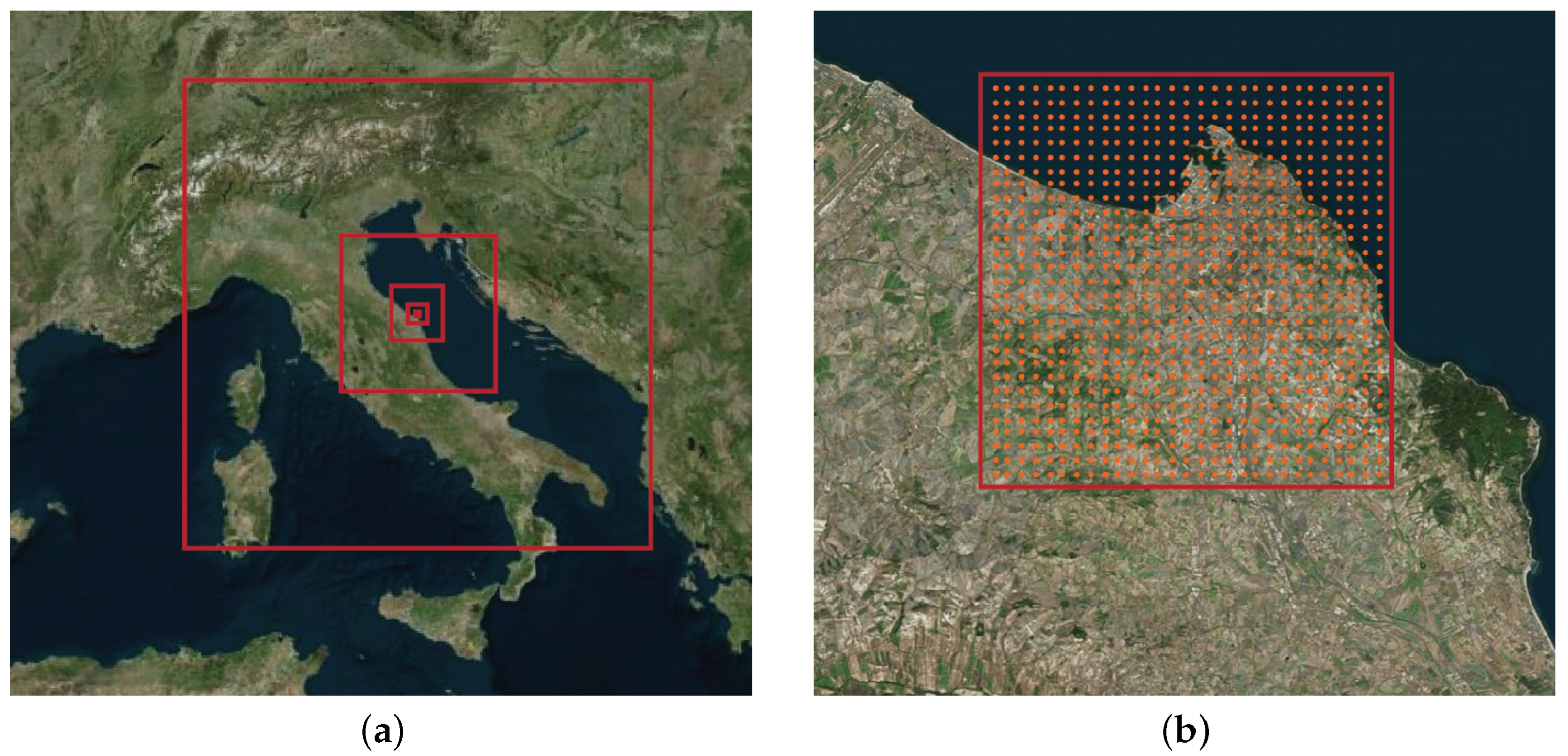
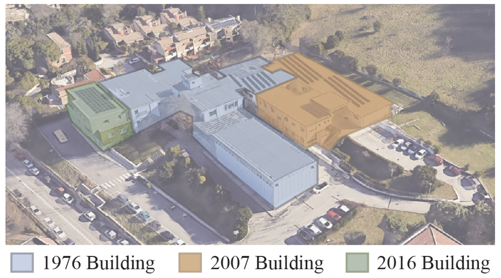
The fourth meteorological dataset is derived from the COordinated Regional Climate Downscaling Experiment regional climate model. This model provides climatic parameters for both the 2015/16 period, aligned with the gas consumption data of the case study, and for future forecasting scenarios. For this analysis, the EUR-11 Domain, the Ensemble RCA4 (r1i1p1) forced by CNRM-CERFACS-CNRM-CM5, and the ALADIN63 RCM model are selected. It facilitates the calculation of variables like total cloud fraction, surface downwelling shortwave radiation, surface air pressure, near-surface air temperature, near-surface relative humidity, near-surface wind speed, eastward near-surface wind, and northward near-surface wind, with a temporal resolution of at least 3 h. This level of frequency is particularly beneficial for building energy simulations, especially when conducting comfort analyses.

The selected experiment corresponds to the RCP4.5 scenario, representing a climate pathway with a radiative forcing level stabilising at 4.5 W/m² before 2100. This scenario aligns with the strategies implemented by major countries to curb greenhouse gas emissions. To evaluate the energy performance of the reference building under future conditions, climatic files are produced by post-processing CORDEX files. This generates three typical meteorological years for the investigated decades: 2025–2035, 2045–2055, and 2065–2075. The process of creating these TMYs, as detailed by Huld et al. [59], follows the ISO 15927-3:2009 normative [60] and the Sandia method [61].

The operational phases are subsequently reported. First, the monthly cumulative distribution function (CDF) is calculated for each physical quantity, month, and year, obtaining the monthly CDF for the individual year. Then, the monthly CDF is defined for every physical quantity and month using the analysed period. The main result of this phase is the long-term monthly CDF.

Table 3. Weather datasets used in this research.

Weather Dataset	Description
Observed_2015–2016	Dataset from November 2015 to April 2016, collected from a weather station in Ancona
DB-IWEC	Default dataset available in DB for Ancona obtained from IWEC
MM5-MRF-NOAH	Dataset from November 2015 to April 2016, extracted with the MRF PBL developed by Hong and Pan, combined with NOAH LSM
CORDEX-CNRM	Dataset from November 2015 to April 2016 and for 2030, 2050, and 2070 TMYs, extracted from the driving model CNRM-CERFACS-CNRM-CM5

summarises the weather datasets used in the present analysis, reporting the name and briefly describing the data source for each climatic file.

5. The Case Study

The selected case study is a primary and nursery school constructed in multiple phases between 1976 and 2016. This building was chosen for its representativeness of Italian educational buildings, reflecting common characteristics found across the country. These include large volumes and standardised layouts, older sections with poor thermal insulation and low-efficiency equipment, and newer areas with more sustainable designs and modern technology. Thanks to its gradual incorporation of different morphological and architectural features, it reflects the evolution of Italy’s educational infrastructure over the years. Moreover, this diversity makes it an exemplary model for examining the effects of climate change and performance improvements achievable through retrofit interventions. For visual reference, Figure 3 provides a schematic representation of the distinct sections that constitute the school.

The oldest part of the building was built in 1976, before the introduction of the first Italian Building Thermal Insulation Regulation [62]. This regulation, mandatory for new constructions, established minimum thermal insulation requirements for both opaque and transparent building elements. The basement area of 130 m² serves technical functions. The larger ground floor (1224.03 m²) houses eight classrooms, two sets of six bathrooms, service rooms, and a gym. The first floor, covering 1118.12 m², contains 13 classrooms along with their associated restrooms. The two-storey building has a reinforced concrete structure and floor slabs made of concrete and brick. The external perimeter incorporates prefabricated elements supported by aluminium frames, divided into upper glazed and lower plastic panel sections. The building lacks thermal insulation, with U-values of 0.88 and 5.78 W/m²K for opaque and single-glazed surfaces, respectively. Heating relies on a natural gas boiler with radiators, while lighting was upgraded to LED in 2010.

In 2007, a new two-storey structure was added. The basement (297.6 m²) includes a computer lab, restrooms, and meeting rooms. The upper floor (718.2 m²) features classrooms, offices, bathrooms, and the Dean’s office with a reception area. This expansion was built using reinforced concrete and introduced an insulated brickwork perimeter. The U-values are 0.71 W/m²K for opaque and 3.09 W/m²K for double-glazed surfaces. Radiators ensure winter comfort, and LED lighting is employed. Furthermore, a 19 kWp photovoltaic generator was installed on the roof.

The most recent section, completed in 2016, adheres to Nearly Zero Energy Building (NZEB) standards. This three-storey building comprises a basement (198.2 m²) hosting the canteen and two upper floors (230.82 m² each) housing classrooms and bathrooms. Constructed with a wooden frame, the building prioritises energy efficiency with low transmittance values. LED lighting and floor heating ensure comfort and energy reduction. The exterior walls boast U-values of 0.15 W/m²K for opaque sections and 0.78 W/m²K for glazed surfaces. For a quick overview,

Table 4. Description of building envelope components and their thermal properties in the original state. For each layer, the values of s (thickness), $\lambda$ (thermal conductivity), and U (thermal transmittance) are shown.

Component		Description
Roof	(a)	1976 and 2007 Building (U = 0.739 W/m2K): 50 mm ceramic clay tile ($\lambda$ = 0.840 W/mK) + 5 mm rubber ($\lambda$ = 0.170 W/mK) + 50 mm insulation ($\lambda$ = 0.080 W/mK) + 10 mm bitumen sheathing ($\lambda$ = 0.500 W/mK) + 40 mm concrete ($\lambda$ = 0.190 W/mK) + 140 mm brick ($\lambda$ = 0.660 W/mK) + 15 mm plasterboard ($\lambda$ = 0.160 W/mK)
	(b)	2016 Building (U = 0.131 W/m2K): 2 mm bitumen sheathing ($\lambda$ = 0.126 W/mK) + 40 mm air gap ($\lambda$ = 0.222 W/mK) + 3 mm insulation ($\lambda$ = 0.003 W/mK) + 50 mm insulation ($\lambda$ = 0.033 W/mK) + 180 mm insulation ($\lambda$ = 0.040 W/mK) + 33 mm wood ($\lambda$ = 0.120 W/mK) + 15 mm plasterboard ($\lambda$ = 0.160 W/mK)
Floor	(c)	1976 and 2007 Building (U = 0.234 W/m2K): 100 mm concrete screed ($\lambda$ = 0.700 W/mK) + 300 mm air gap ($\lambda$ = 0.222 W/mK) + 100 mm concrete slab ($\lambda$ = 0.700 W/mK) + 80 mm insulation ($\lambda$ = 0.034 W/mK) + 80 mm concrete ($\lambda$ = 1.400 W/mK) + 15 mm ceramic tile ($\lambda$ = 1.400 W/mK)
	(d)	2016 Building (U = 0.190 W/m2K): 100 mm concrete screed ($\lambda$ = 0.700 W/mK) + 300 mm air gap ($\lambda$ = 0.222 W/mK) + 200 mm concrete slab ($\lambda$ = 0.660 W/mK) + 40 mm concrete ($\lambda$ = 2.500 W/mK) + 80 mm insulation ($\lambda$ = 0.035 W/mK) + 100 mm concrete ($\lambda$ = 0.190 W/mK) + 12 mm insulation ($\lambda$ = 0.030 W/mK) + 18 mm concrete ($\lambda$ = 1.400 W/mK) + 15 mm ceramic tile ($\lambda$ = 1.300 W/mK)
Ext. wall	(e)	1976 Building (U = 0.876 W/m2K): 15 mm solid lime plaster ($\lambda$ = 0.160 W/mK) + 120 mm solid brick burned ($\lambda$ = 0.427 W/mK) + 70 mm air gap ($\lambda$ = 0.222 W/mK) + 80 mm solid brick burned ($\lambda$ = 0.427 W/mK) + 15 mm solid lime plaster ($\lambda$ = 0.160 W/mK)
	(f)	2007 Building (U = 0.712 W/m2K): 15 mm solid lime plaster ($\lambda$ = 0.160 W/mK) + 120 mm solid brick burned ($\lambda$ = 0.427 W/mK) + 50 mm air gap ($\lambda$ = 0.222 W/mK) + 80 mm solid brick burned ($\lambda$ = 0.427 W/mK) + 30 mm insulation ($\lambda$ = 0.085 W/mK) + 15 mm solid lime plaster ($\lambda$ = 0.160 W/mK)
	(g)	2016 Building (U = 0.154 W/m2K): 5 mm solid lime plaster ($\lambda$ = 0.300 W/mK) + 40 mm insulation ($\lambda$ = 0.034 W/mK) + 200 mm wood ($\lambda$ = 0.012 W/mK) + 120 mm insulation ($\lambda$ = 0.039 W/mK) + 0.5 mm vapour barrier ($\lambda$ = 0.500 W/mK) + 40 mm air gap ($\lambda$ = 0.222 W/mK) + 20 mm wood ($\lambda$ = 0.012 W/mK) + 15 mm plasterboard ($\lambda$ = 0.250 W/mK)
Int. wall	(h)	1976 and 2007 Building (U = 1.575 W/m2K): 15 mm solid lime plaster ($\lambda$ = 0.160 W/mK) + 80 mm solid brick burned ($\lambda$ = 0.427 W/mK) + 15 mm solid lime plaster ($\lambda$ = 0.160 W/mK)
	(i)	2016 Building (U = 0.301 W/m2K): 260 mm plasterboard ($\lambda$ = 0.250 W/mK) + 100 mm insulation ($\lambda$ = 0.035 W/mK) + 260 mm plasterboard ($\lambda$ = 0.250 W/mK)
Window	(j)	Window_1976 Building (U = 5.778 W/m2K): 6 mm single clear glazing ($\lambda$ = 0.900 W/mK)
	(k)	2007 Building (U = 3.094 W/m2K): 6 mm single clear glazing ($\lambda$ = 0.900 W/mK) + 6 mm air gap ($\lambda$ = 0.026 W/mK) + 6 mm single clear glazing ($\lambda$ = 0.900 W/mK)
	(l)	2016 Building (U = 0.780 W/m2K): 3 mm single clear glazing ($\lambda$ = 0.900 W/mK) + 13 mm argon gap ($\lambda$ = 0.017 W/mK) + 3 mm single clear glazing ($\lambda$ = 0.900 W/mK)

summarises the thermal properties of the building envelope.

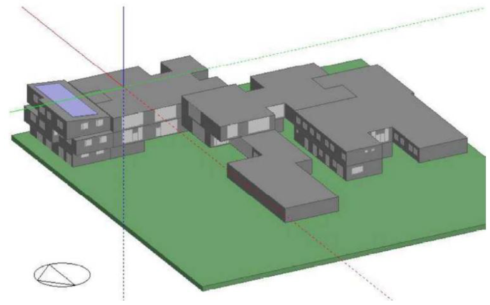
Building Energy Modelling and Validation

Energy simulations were performed by modelling the detailed HVAC system. The choice of properly inserting the building equipment according to the information previously reported aims to enhance analysis precision. In detail, a group of different zones for each building section, including both rooms and corridors, was created, and the specific functional equipment template was assigned considering HVAC characteristics. Furthermore, the settings of every heating component were defined on the base of the collected data to achieve alignment between the modelled HVAC system and the actual setup.

To better reflect real-world usage of interior spaces, schedules were aligned with the official school calendar, and a personnel interview was carried out to identify extra-curricular activities, enhancing the authenticity of the simulation (see

Table 5. Building energy simulation occupancy schedule.

Month	Monday to Friday	Weekend
January to June	8:20–16:20	Off
July and August	Off	Off
September to December	8:20–16:20	Off
National and Local Holidays	Off	Off

for more details).

As previously outlined, both the 1976 and 2007 buildings share a heating system without any cooling provisions. The winter heating temperature is maintained at 20 °C, and this setpoint remains constant due to the absence of retrofitted control systems. The heating plant operates using a simple on/off control strategy, following a predefined schedule (see

Table 6. Operative schedule of the heating system.

Time Period	00:00–06:00	06:00–18:00	18:00–24:00
15 November–30 April	Off	On	Off
1 May–14 November	Off	Off	Off
Weekends	Off	Off	Off
National and Local Holidays	Off	Off	Off

). No ventilation system is installed in any of the school buildings. Finally, the model sets the infiltration rate at the average value of 0.6 ac/h, slightly modified according to the specific simulation period in order to consider both the building’s geometry and the occupancy of the spaces by the students. Figure 4 shows the energy model elaborated for the analyses.

A validation process is crucial for an accurate estimation of the case study’s energy performance. Thus, the gas bills from September 2015 to August 2016 are compared with estimated energy consumption derived from a climatic file containing measured data for the same year (the SIRMIP database), following the ASHRAE guideline 14 criteria [63]. Notably, the validation specifically excluded the 2016 building since it was inaugurated after the analysed period.

Figure 5 and Figure 6 illustrate the monthly and annual gas energy consumption data obtained from both estimated and measured values. Error bars, set at 10%, are inserted as inferior and superior limits. Overall, the model effectively reflects the building’s energy needs. For almost all the months analysed, the estimated consumption closely matches the actual bills. However, there are some deviations: it tends to overestimate by up to 9% in November and underestimate by up to 2% in February.

Particularly significant fluctuations occur during transitional months like April, where the model underestimates actual consumption by 51%. This variance can be attributed to the impact of user behaviour on indoor space requirements, a factor that studies have shown to vary unpredictably in real-world settings, making it difficult to accurately model with simulation tools [64,65]. This discrepancy is particularly pronounced during transitional seasons, such as spring, and in April. For instance, Pisello et al. [66] found that the average daily window opening hours are significantly higher in spring than in other seasons, contributing to increased variability in energy demand. Additionally, the anomaly may also stem from common energy management practices in public buildings in Italy, where contractors often bypass thermoregulation systems. Instead of adjusting heating or cooling dynamically to external temperatures, they frequently operate the systems on fixed schedules, as required by national regulations [51]. This rigid approach further exacerbates energy inefficiencies during transitional periods, such as in April, when external temperatures fluctuate significantly.

A similar correspondence extends to annual simulation, with minor differences (see Figure 6). In this case, the model annually underestimates 4% of the actual energy consumption. Based on these results, the model is considered well-calibrated, effectively describing the case study’s energy performance.

Then, dynamic energy simulations were conducted to better understand how historical, current, and future weather conditions impact buildings. These simulations involve comparing outputs obtained by employing various climatic files, allowing researchers to assess the varying effects of different weather conditions on buildings’ energy performance. Furthermore, conducting simulations on a case study comprising buildings from various construction periods enables a more thorough assessment of their responsiveness to climatic factors.

6. Results and Discussion

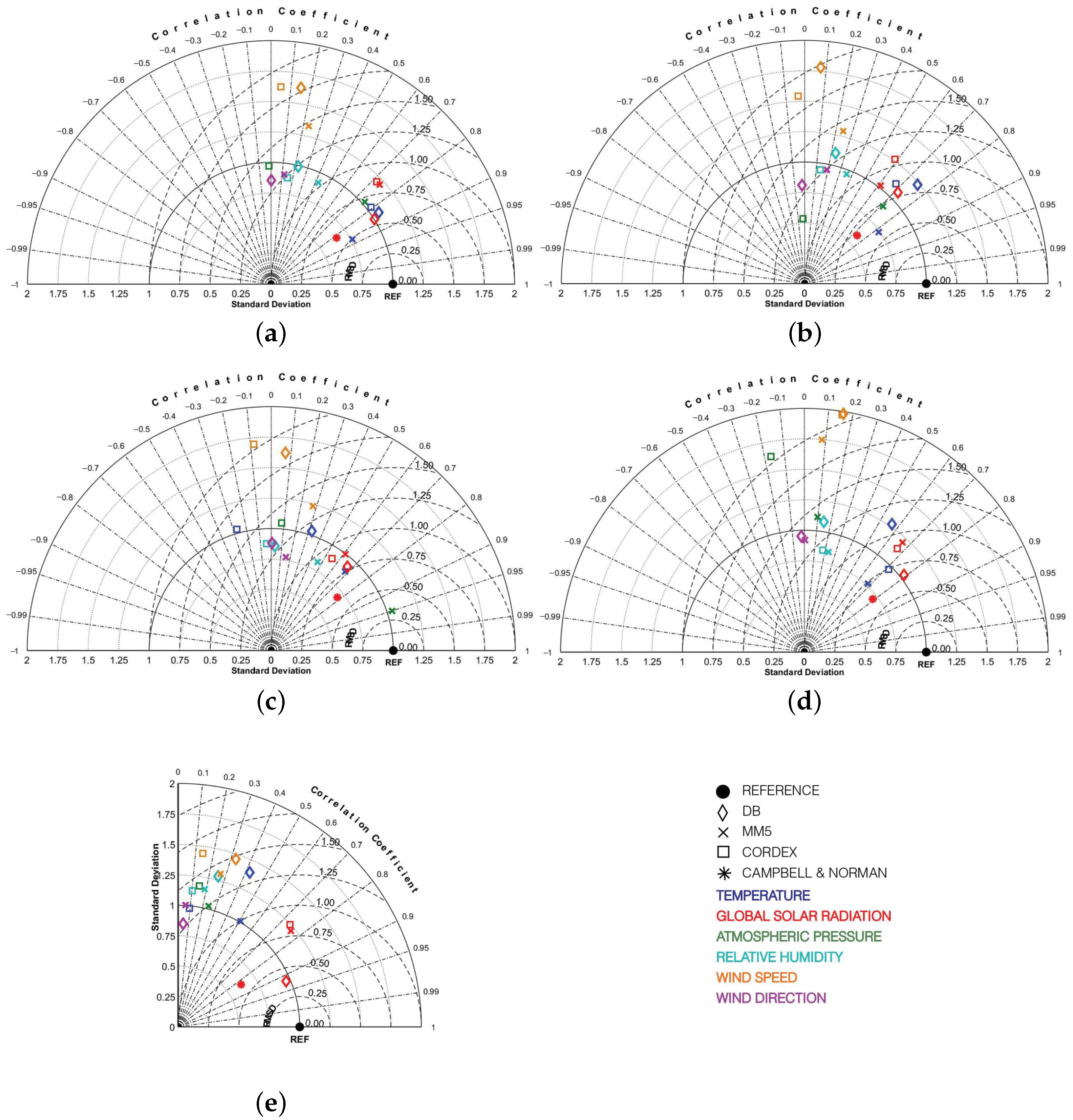
6.1. Intercomparisons among Weather Datasets

The selected historical and current climatic files are compared in terms of temperature, global solar radiation, atmospheric pressure, relative humidity, and wind speed and direction. The adopted reference pattern is derived from the SIRMIP meteorological mast.

Figure 7 depicts the Taylor diagrams generated from both seasonal and annual data. Seasons are defined according to the Italian astronomical seasons: spring from 21/03 to 20/06, summer from 21/06 to 20/09, autumn from 21/09 to 20/12, and winter from 21/12 to 20/03.

Focusing on the annual dataset (Figure 7a), it becomes evident that temperature and global solar radiation are the climatic parameters better described by the investigated databases. The temperature values (blue markers in the chart) present a correlation coefficient ranging from 0.79 for the CORDEX dataset to 0.88 for the MM5 dataset. Additionally, good standard deviations and centred root-mean-square differences are calculated for this variable. A similar pattern is observed for solar radiation, which is well predicted by all sources, particularly by the DB dataset. Conversely, the two regional models exhibit similar but lower performance. Moreover, Campbell and Norman’s approach provides estimations for this parameter with good correlation coefficients, standard deviations, and RMSD, respectively, equal to 0.81, 0.65, and 0.60. Atmospheric pressure (green markers in the chart) is only compared for the MM5 and CORDEX datasets because DB assumes a constant value equal to 101,181 Pa, rendering it incomparable with specific measured data. Among the two options, MM5 better describes the variability of this parameter with a correlation coefficient of 0.75, a standard deviation of 1.04, and an RMSD of 0.71. Conversely, CORDEX exhibits less accurate statistical parameters. Relative humidity and wind speed (light blue and yellow markers in the chart, respectively) are represented similarly by DB and CORDEX, although they demonstrate different predictive capabilities for the two variables. MM5 shows greater accuracy in estimating these parameters, with correlation coefficients of 0.43 for relative humidity and 0.23 for atmospheric pressure, along with standard deviations of 0.90 and 1.35 and RMSDs of 1.05 and 1.45, respectively. Lastly, wind direction (purple markers) is predicted by DB and MM5, while CORDEX lacks this parameter. The regional climate model demonstrates a better predictive capability than the DB source, showing slightly higher accuracy in estimating this parameter with better correlations. However, wind direction is generally predicted with the lowest precision due to its changing nature and the difficulties in calculating or recording with good approximation.

The observations made for the annual dataset can be extended to the seasonal charts with only a few differences. Temperature and global solar radiation are better described by all sources, although DB and CORDEX exhibit less accuracy during extreme weather conditions, such as those expected in winter (Figure 7c) and summer (Figure 7e). Conversely, MM5 improves its capability to calculate temperature fields on a seasonal scale. Solar radiation performance remains consistent across seasons, with the DB database expected to perform best during summertime. Moreover, Campbell and Norman’s method proves to be a valid option for estimating seasonal global solar radiation values. Similarly, MM5 predicts atmospheric pressure better than CORDEX, particularly in spring (Figure 7d), when the latter model performs poorly. The findings regarding relative humidity and wind speed are confirmed on a seasonal scale, with less accuracy expected in predicting wind speed during spring. Lastly, wind direction is calculated with similar precision by DB and MM5 across seasonal datasets.

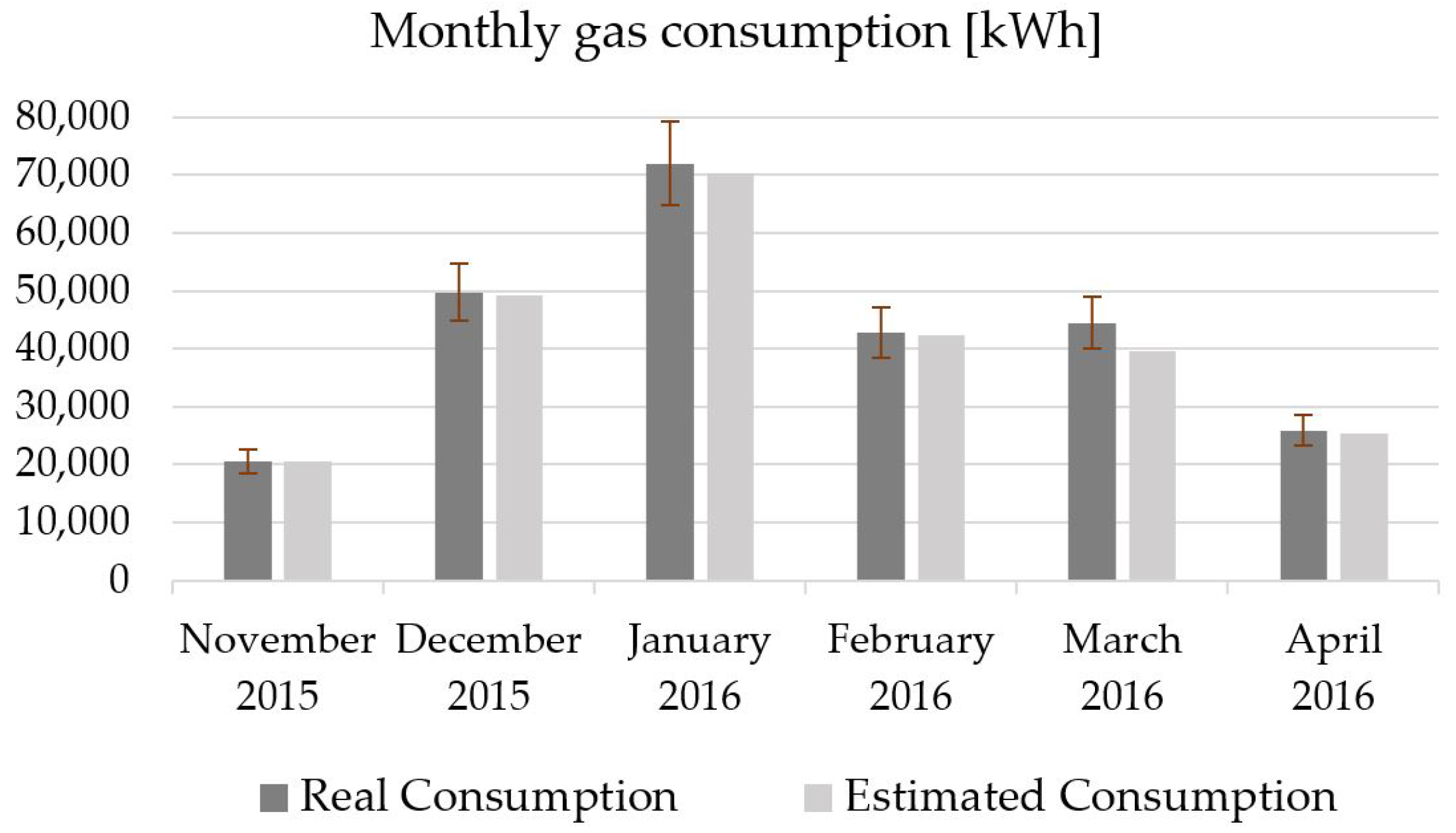
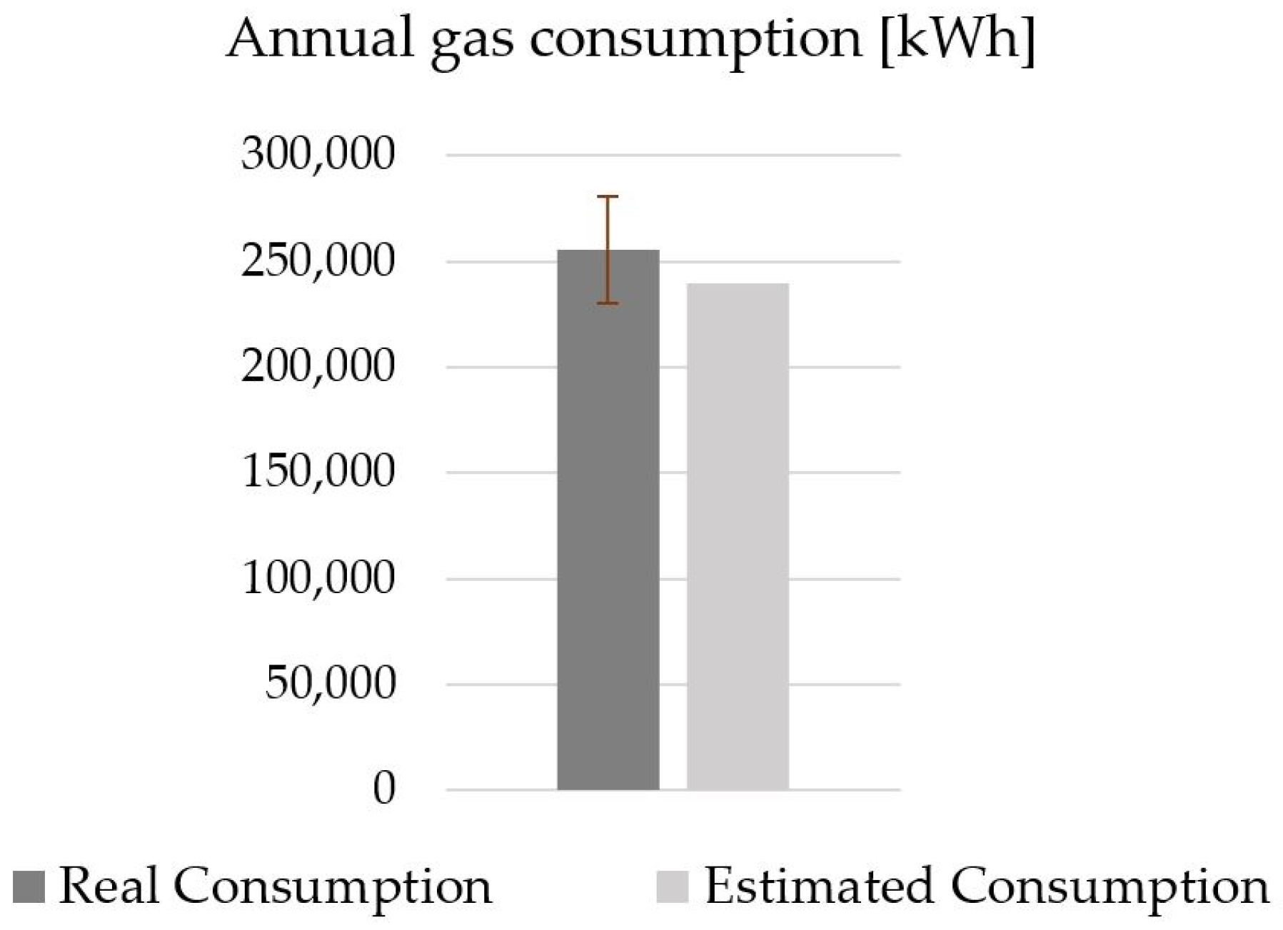
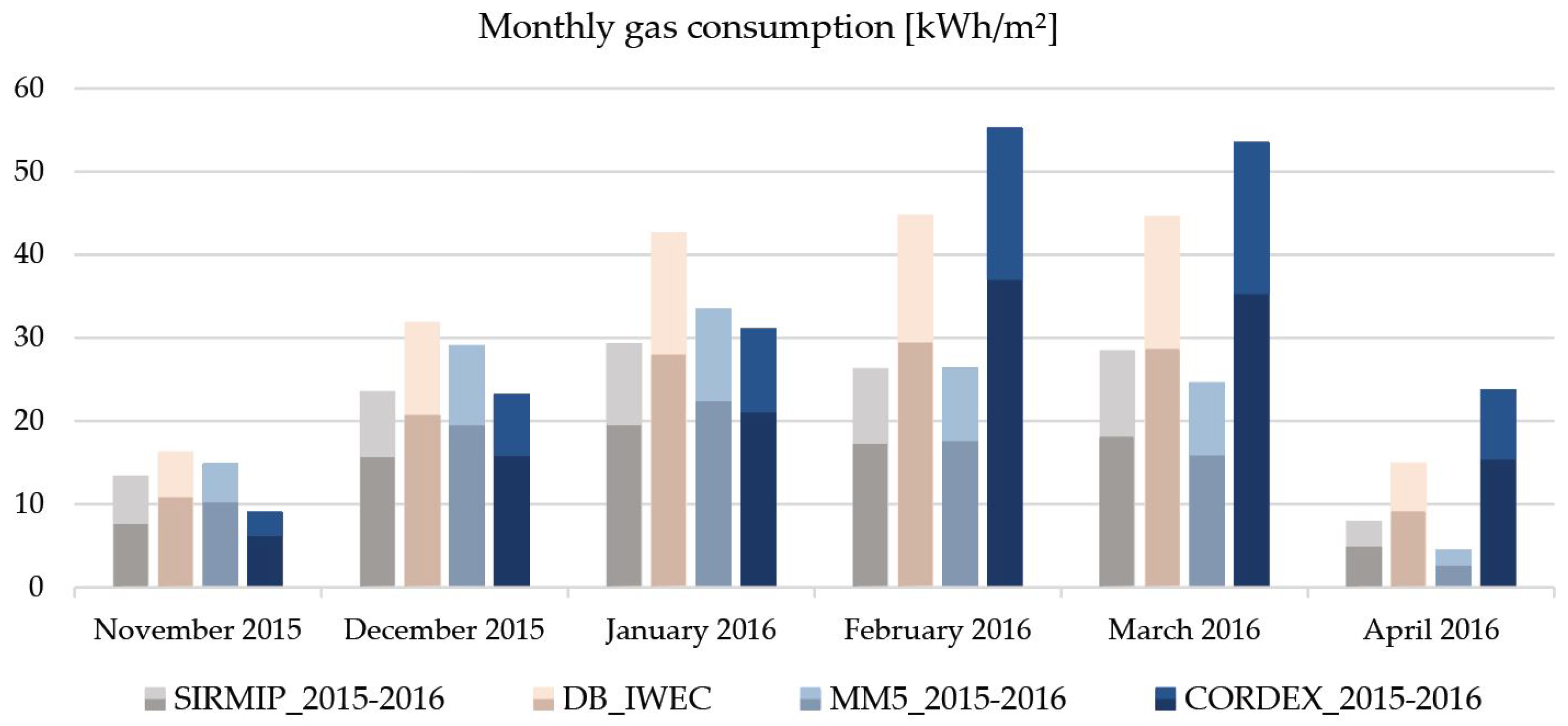
6.2. Dynamic Energy Simulations under Historical and Present Climate Conditions

Considering the energy efficiency of the newest part of the building and the different sources of energy, the simulations conducted here simultaneously incorporate the sections built in 1976 and 2007 into one scenario and only the 2016 section in another. This approach aims to compare gas consumption for older buildings with electricity production/requirements for new ones. The energy consumption, expressed on both monthly and annual scales, is assessed in kWh/m².

Examining the seasonal and annual gas consumption, depicted in Figure 8 and Figure 9, respectively, it is noteworthy that, as expected, the 1976 building exhibits higher energy requirements than the newer building. Specifically, monthly consumption ranges from 29% (in April) to 54% (in November), assuming the MM5 climatic database surpasses the other section. Annually, a similar discrepancy is anticipated between the two buildings, with a maximum value of +50% predicted using CORDEX data.

The comparison of estimates derived from different climatic inputs underscores the impact of these parameters on the predictions. When considering the SIRMIP dataset as a reference, given its reliance on measured values, the DB dataset tends to significantly overestimate global monthly consumption, particularly from January (+46%) to April (+88%). This overestimation arises from the higher average temperatures assumed, leading to increased energy demands for maintaining comfortable conditions.

Similar discrepancies are observed with the CORDEX dataset, which markedly overcalculates energy consumption, especially in February (+110%), March (+88%), and April (+199%). For the remaining months, the dataset underestimates from −33% in November to −1% in December. It is important to note that this dataset consists of 3-hour estimations and, consequently, may not accurately capture temporal fluctuations. The MM5 regional climate model, in contrast to the others, aligns more closely with the SIRMIP consumption, except for April, which shows a significant deviation (approximately −70%).

Extending the analysis to the annual scale (Figure 9), the observed trend remains consistent. The MM5 dataset continues to demonstrate more accurate performance compared to the historical DB dataset and the other virtual anemometer, with an error of +3%. However, more substantial variations are expected with the DB and CORDEX databases, which predict higher gas consumption of about +51% and +52%, respectively. Based on these results, the general tendency to adopt DB weather files for building evaluation and calibration reveals limitations, mainly because the data are historical and not representative of a specific current year.

In addition to the considerations discussed in the earlier parts of the case study, evaluating the impact of different climatic files on an energy-efficient NZEB building is valuable. Here, the energy requirement is assessed based on electricity consumption per square metre.

The chart shown in Figure 10 and Figure 11 indicates that the energy requirement of the newest section of the building is significantly lower than that of the older sections. Specifically, the newest part uses an average of 3.43 kWh/m² per month, compared to 17.93 kWh/m² for the 1976 section and 9.29 kWh/m² for the 2007 section. Moreover, the NZEB building demonstrates less sensitivity to different climatic files, showing minor variability across the analysed datasets. The DB file generally overestimates the building’s energy performance, while the MM5 dataset consistently proves to be the most accurate in representing real conditions. In contrast, CORDEX mostly overestimates energy consumption.

On an annual scale (see Figure 11), the differences in both energy generation and consumption become less pronounced. The variation ranges from −0.1% with the MM5 file to +7% under CORDEX climate data and from −10% with DB to 23% with CORDEX compared to the SIRMIP output for both energy consumed and produced.

It is important to note that these results are compared in terms of energy requirement per square metre, despite being related to different energy sources, which is in line with the comparative purpose of this work.

6.3. The Impact of Climate Change on Energy Retrofit Solutions

The building’s energy retrofit primarily aimed to decrease heat loss through its envelope significantly. This choice comes from the consciousness that interventions on the building envelope (insulation of external walls, roofs and floors, windows, etc.) are the most effective in increasing energy performance, and for this reason, they are largely adopted, as underlined by the literature review [67,68,69].

The approach taken for the retrofit was guided by the constraints outlined in the Directive 2002/91/UE [70] and its recasts [71,72] (implemented in Italy through various Legislative Decrees [73,74,75].

Different insulation materials, both natural and synthetic, are considered to meet the standard limitations. Thus, EPS and glass wool insulation are chosen for evaluation. Furthermore, a key aspect of the retrofit involves upgrading the inadequate glazed surfaces with more efficient double-glazed windows and PVC frames for both the 1976 and 2007 sections. Consequently, the transmittance values for the transparent surfaces and frames are reduced to recommended levels of 1.49 W/m²K and 3.48 W/m²K, respectively. A simplified representation of the retrofitted components is outlined in

Table 7. Description of the building’s components and their thermal properties for the 1976 building.

(a)	Ext. wall_1976 Building—EPS retrofit solution (U = 0.229 W/m2K): 2 mm solid lime plaster (λ = 0.300 W/mK) + 8 mm cement plaster (λ = 500.000 W/mK) + 100 mm EPS insulation (λ = 0.031 W/mK) + 8 mm cement plaster (λ = 500.000 W/mK) + 15 mm solid lime plaster (λ = 0.160 W/mK) + 120 mm solid brick burned (λ = 0.427 W/mK) + 70 mm air gap (λ = 0.222 W/mK) + 80 mm solid brick burned (λ = 0.427 W/mK) + 15 mm solid lime plaster (λ = 0.160 W/mK)
(b)	Ext. wall_1976 Building—Glass wool retrofit solution (U = 0.244 W/m2K): 2 mm solid lime plaster ($\lambda$ = 0.300 W/mK) + 8 mm cement plaster ($\lambda$ = 500.000 W/mK) + 100 mm glass wool insulation ($\lambda$ = 0.034 W/mK) + 4 mm cement plaster ($\lambda$ = 500.000 W/mK) + 15 mm solid lime plaster ($\lambda$ = 0.160 W/mK) + 120 mm solid brick burned ($\lambda$ = 0.427 W/mK) + 70 mm air gap ($\lambda$ = 0.222 W/mK) + 80 mm solid brick burned ($\lambda$ = 0.427 W/mK) + 15 mm solid lime plaster ($\lambda$ = 0.160 W/mK)
(c)	Ext. wall_2007 Building—EPS retrofit solution (U = 0.250 W/m2K): 2 mm solid lime plaster ($\lambda$ = 0.300 W/mK) + 8 mm cement plaster ($\lambda$ = 500.000 W/mK) + 80 mm EPS insulation ($\lambda$ = 0.031 W/mK) + 15 mm solid lime plaster ($\lambda$ = 0.160 W/mK) + 120 mm solid brick burned ($\lambda$ = 0.427 W/mK) + 50 mm air gap ($\lambda$ = 0.222 W/mK) + 80 mm solid brick burned ($\lambda$ = 0.427 W/mK) + 15 mm solid lime plaster ($\lambda$ = 0.160 W/mK)
(d)	Ext. wall_2007 Building—Glass wool retrofit solution (U = 0.229 W/m2K): 2 mm solid lime plaster ($\lambda$ = 0.300 W/mK) + 8 mm cement plaster ($\lambda$ = 500.000 W/mK) + 100 mm glass wool insulation ($\lambda$ = 0.034 W/mK) + 15 mm solid lime plaster ($\lambda$ = 0.160 W/mK) + 120 mm solid brick burned ($\lambda$ = 0.427 W/mK) + 50 mm air gap ($\lambda$ = 0.222 W/mK) + 80 mm solid brick burned ($\lambda$ = 0.427 W/mK) + 30 mm insulation ($\lambda$ = 0.085 W/mK) + 15 mm solid lime plaster ($\lambda$ = 0.160 W/mK)
(e)	Window_1976 and 2007 Building (U = 1.493 W/m2K): 6 mm single clear glazing ($\lambda$ = 0.900 W/mK) + 13 mm argon gap ($\lambda$ = 0.017 W/mK) + 6 mm glass wool insulation ($\lambda$ = 0.034 W/mK) + 6 mm single clear glazing ($\lambda$ = 0.900 W/mK)

to provide a clear overview. It is important to underline that the newest section of the school is analysed in the current state, and no intervention is evaluated considering its high energy efficiency.

Figure 12 depicts the estimated annual heating consumption for the two sections of the case study, considering both the current configuration and the upgraded energy-efficient state under future climate conditions. Although the CORDEX model is less accurate in estimating weather variables, as discussed in previous sections, it remains a valuable option for predicting these parameters for the future. Therefore, it is essential for this in-depth study.

Also, in this case, the darkest part of the bar represents the 1976 building, while the lighter part describes the 2007 section. Moreover,

Table 8. Expected mean, minimum, and maximum temperatures associated with each dataset.

Climate Database	Tmean [°C]	Tmin [°C]	Tmax [°C]
SIRMIP	9.45	−6.10	25.60
CORDEX_2030	9.68	−3.60	20.00
CORDEX_2050	10.21	−0.80	23.20
CORDEX_2070	10.18	+0.42	20.00

shows the mean, minimum, and maximum temperature values associated with each climatic dataset to better understand the expected variations due to future conditions.

The results indicate that the anticipated rise in temperatures will reduce heating demands. This effect becomes more pronounced by 2070, with a decrease of approximately 25% for the current building configuration and a 30% reduction for the upgraded version compared to their respective 2030 benchmarks.

Under current climate conditions, the section with the poorest energy performance (the 1976 building) significantly impacts overall gas consumption, accounting for about 66% of the total building needs across all analysed years. The implementation of an insulated layer and the replacement of subpar glazed surfaces result in substantial improvements in the building’s overall energy performance. The examined solutions show nearly identical effects for both buildings. Using glass wool leads to reductions of approximately 54%, 50%, and 57% for 2030, 2050, and 2070, respectively, compared to the original versions for those years. Alternatively, the EPS approach demonstrates slightly superior results, yielding reductions of roughly 53% for 2030 and 2050 and 57% for 2070.

Considering future climate conditions, the 2016 building exhibits negligible variations compared to its current performance, as reported in Figure 13. The energy consumption shows only slight changes from the current electrical requirement of 20.15 kWh/m² to 20.51 kWh/m², 20.28 kWh/m², and 20.21 kWh/m² projected for 2030, 2050, and 2070, respectively. A such future reduction from 2030 to 2070 is related to higher expected mean temperatures and, consequently, lower building energy requirements. A similar trend is observed for energy generation, which is expected to generally increase under future climate conditions, especially for 2050 and 2070.

The obtained results indicate that the energy efficiency of this building section ensures reduced vulnerability to climate change.

7. Conclusions

This study assessed the impact of different climate datasets on dynamic energy simulations and evaluated the adaptation of an educational building in Central Italy to climate change. By comparing historical, current, and future climatic scenarios, the building’s heating demands were estimated both in its current state and after a proposed energy-efficient retrofit.

In the first phase, both measured and model-generated meteorological datasets were collected and compared to assess their accuracy in predicting key weather parameters like solar radiation, temperature, atmospheric pressure, humidity, wind speed, and wind direction. Different methods for calculating global solar radiation were also tested. The next phase focused on evaluating the energy performance of the reference building and determining its vulnerability to the effects of climate change.

The main conclusions of the investigation are summarised as follows:

• The MM5 dataset proved most reliable for predicting key weather parameters. The DB dataset also showed good performance, especially in estimating solar radiation on both annual and seasonal scales. Moreover, the Campbell and Norman approach was effective for calculating solar parameters, although it slightly underestimated variability.
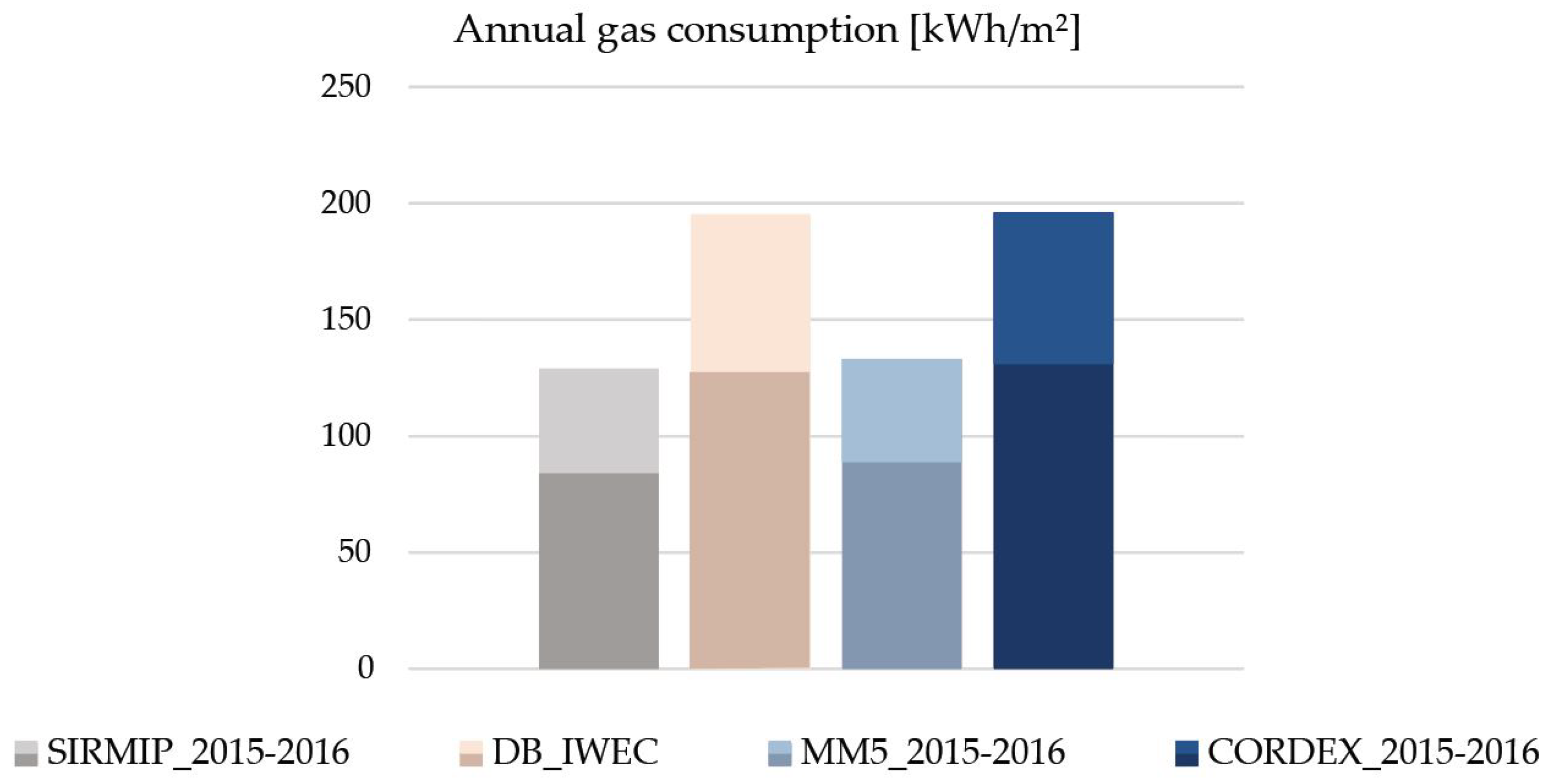
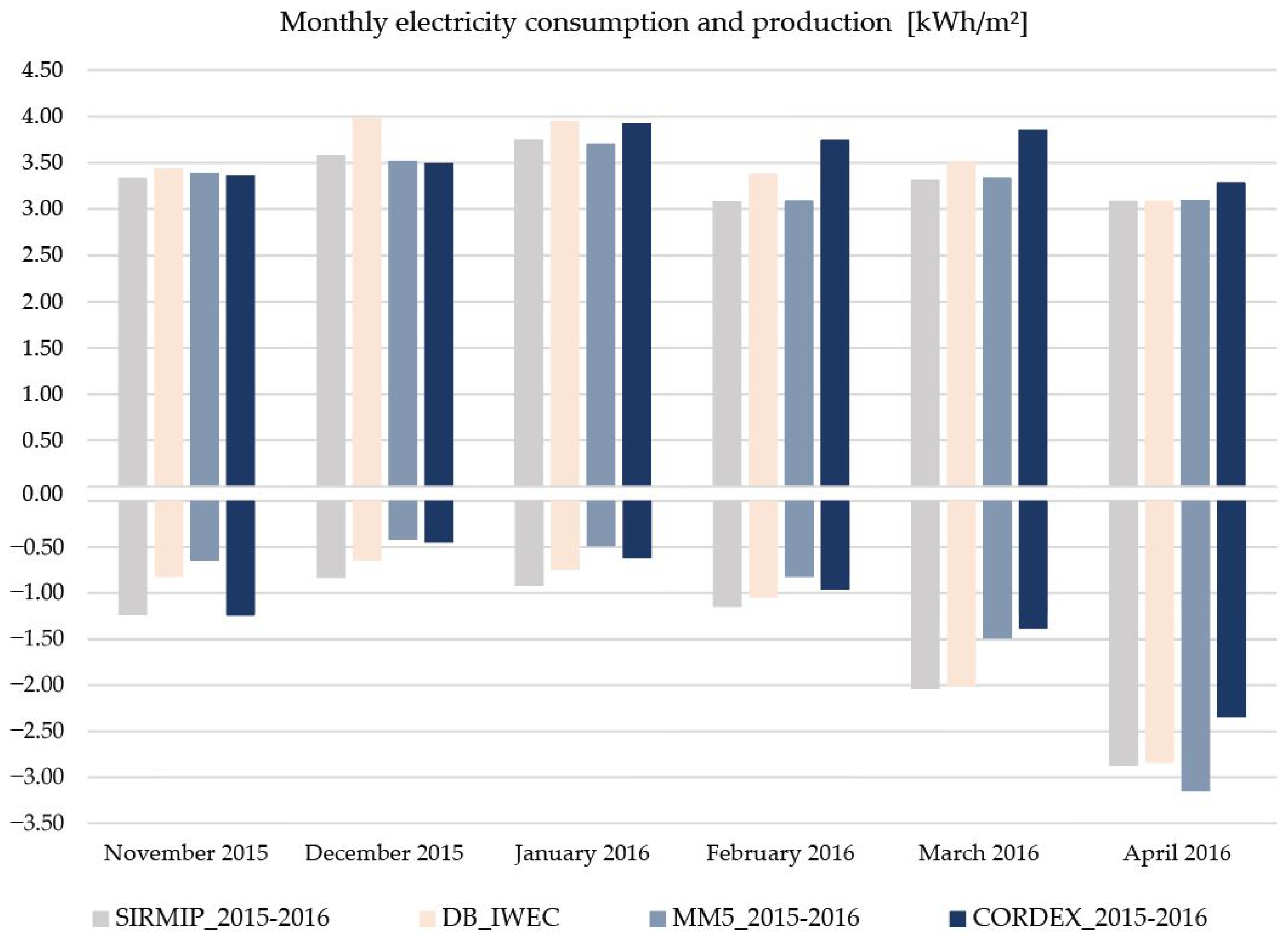
• Energy performance analysis revealed that the older 1976 building section required significantly more energy than newer sections, with monthly consumption differences ranging from 29% to 54% higher. The MM5 dataset providing the most accurate consumption estimates, closely aligning with measured data except for notable deviations in April. The DB and CORDEX databases often overestimated energy consumption, mispredicting monthly values by up to 88% and 199%, respectively.
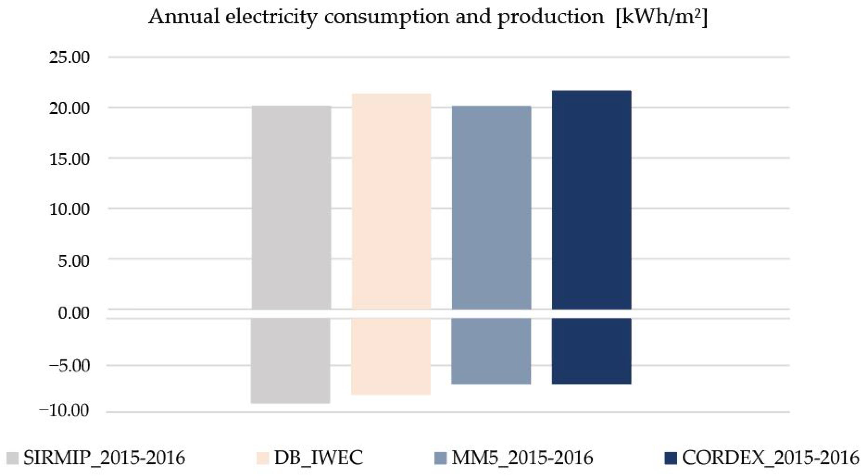
• Energy requirements for the newer NZEB building were significantly lower and showed less sensitivity to different climatic datasets. Again, the MM5 dataset proved to be the most accurate, while DB data generally overestimated energy consumption.
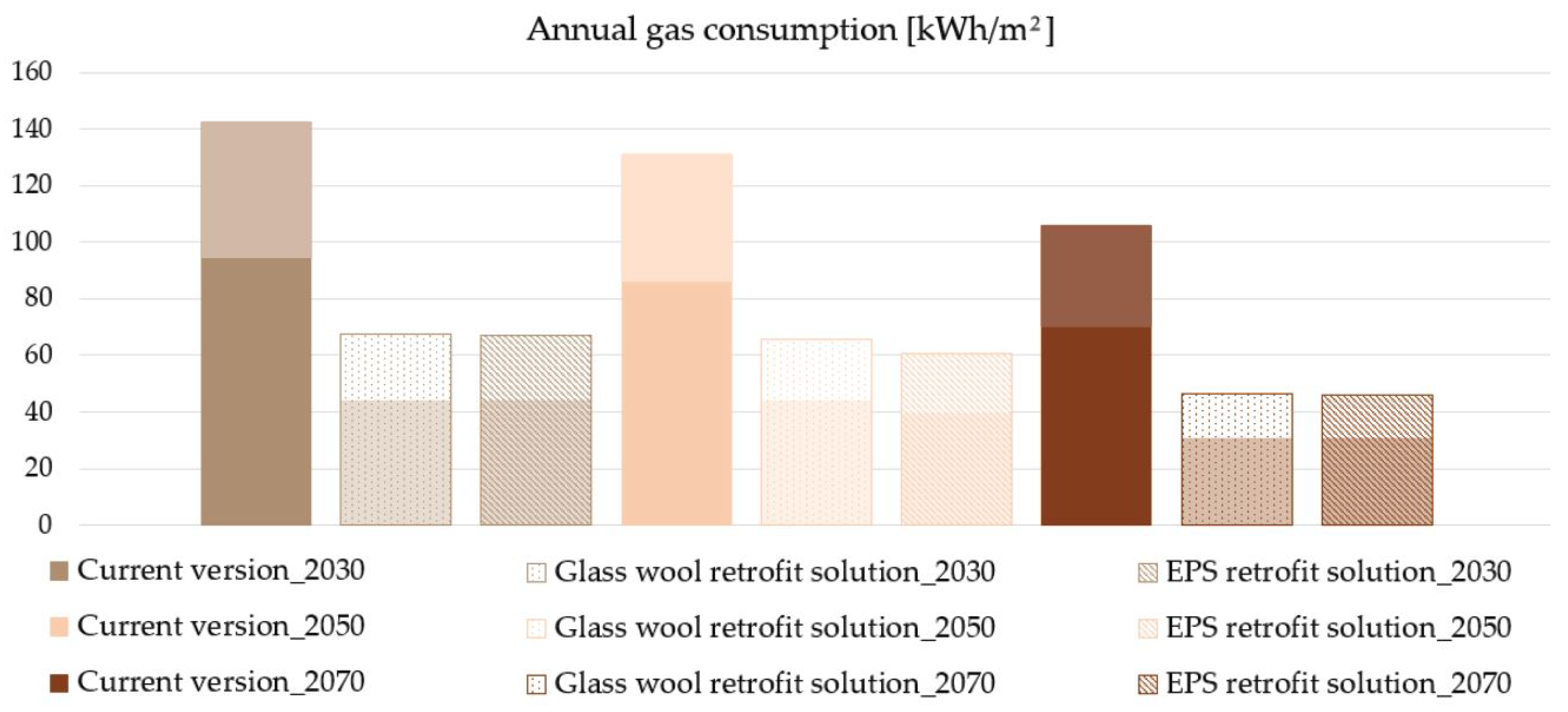
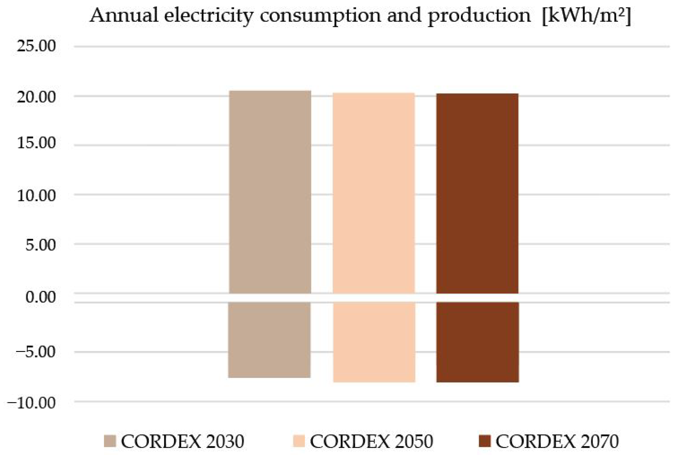
• Retrofitting with EPS and glass wool insulation, along with window replacements, showed notable energy reductions in future climate scenarios, with EPS slightly outperforming glass wool. Under future climate conditions, the energy consumption of the 2016 building section is expected to remain stable or slightly decrease due to higher mean temperatures, indicating the building’s resilience to climate change.

While this study offers valuable insights into the impact of climatic datasets on energy simulations and demonstrates that targeted building retrofits, particularly high-performance insulation and window upgrades, can significantly enhance energy efficiency and resilience to future climate conditions, certain limitations must be acknowledged. First, the study’s analysis was based on a restricted selection of climatic datasets and time periods, which may affect the generalisability of the results to other geographical regions. Additionally, the focus was primarily on heating demand, with no consideration of cooling requirements, which are likely to become increasingly important as temperatures rise in future climate scenarios.

Additional research should address these limitations and investigate hybrid approaches that combine multiple datasets or incorporate machine learning techniques capable of further improving the accuracy of energy performance simulations. Moreover, assessing the impact of other retrofit strategies, such as integrating renewable energy or advanced materials, would offer a more comprehensive approach to enhancing energy efficiency across diverse climates.

References

1. European Union. Manual for Statistics on Energy Consumption in Households; Publications Office of the European Union: Luxembourg, 2013; 170p. [Google Scholar]
2. World Green Building Council. World Green Building Council Annual Report 2020; World Green Building Council: London, UK, 2020; pp. 1–22. [Google Scholar]
3. Yau, Y.; Hasbi, S. A review of climate change impacts on commercial buildings and their technical services in the tropics. Renew. Sustain. Energy Rev. 2013, 18, 430–441. [Google Scholar] [CrossRef]
4. Berger, T.; Amann, C.; Formayer, H.; Korjenic, A.; Pospischal, B.; Neururer, C.; Smutny, R. Impacts of climate change upon cooling and heating energy demand of office buildings in Vienna, Austria. Energy Build. 2014, 80, 517–530. [Google Scholar] [CrossRef]
5. Zheng, Y.; Weng, Q. Modeling the effect of climate change on building energy demand in Los Angeles county by using a GIS-based high spatial- and temporal-resolution approach. Energy 2019, 176, 641–655. [Google Scholar] [CrossRef]
6. Clarke, L.; Eom, J.; Marten, E.H.; Horowitz, R.; Kyle, P.; Link, R.; Mignone, B.K.; Mundra, A.; Zhou, Y. Effects of long-term climate change on global building energy expenditures. Energy Econ. 2018, 72, 667–677. [Google Scholar] [CrossRef]
7. Zhu, M.; Pan, Y.; Huang, Z.; Xu, P. An alternative method to predict future weather data for building energy demand simulation under global climate change. Energy Build. 2016, 113, 74–86. [Google Scholar] [CrossRef]
8. Dodoo, A.; Gustavsson, L.; Bonakdar, F. Effects of Future Climate Change Scenarios on Overheating Risk and Primary Energy Use for Swedish Residential Buildings. Energy Procedia 2014, 61, 1179–1182. [Google Scholar] [CrossRef]
9. Verichev, K.; Zamorano, M.; Carpio, M. Effects of climate change on variations in climatic zones and heating energy consumption of residential buildings in the southern Chile. Energy Build. 2020, 215, 109874. [Google Scholar] [CrossRef]
10. Ciancio, V.; Salata, F.; Falasca, S.; Curci, G.; Golasi, I.; de Wilde, P. Energy demands of buildings in the framework of climate change: An investigation across Europe. Sustain. Cities Soc. 2020, 60, 102213. [Google Scholar] [CrossRef]
11. Shen, P. Impacts of climate change on U.S. building energy use by using downscaled hourly future weather data. Energy Build. 2017, 134, 61–70. [Google Scholar] [CrossRef]
12. Zhai, Z.J.; Helman, J.M. Implications of climate changes to building energy and design. Sustain. Cities Soc. 2019, 44, 511–519. [Google Scholar] [CrossRef]
13. Kikumoto, H.; Ooka, R.; Arima, Y.; Yamanaka, T. Study on the future weather data considering the global and local climate change for building energy simulation. Sustain. Cities Soc. 2015, 14, 404–413. [Google Scholar] [CrossRef]
14. Shibuya, T.; Croxford, B. The effect of climate change on office building energy consumption in Japan. Energy Build. 2016, 117, 149–159. [Google Scholar] [CrossRef]
15. Huang, J.; Gurney, K.R. The variation of climate change impact on building energy consumption to building type and spatiotemporal scale. Energy 2016, 111, 137–153. [Google Scholar] [CrossRef]
16. Yau, Y.; Hasbi, S. A Comprehensive Case Study of Climate Change Impacts on the Cooling Load in an Air-Conditioned Office Building in Malaysia. Energy Procedia 2017, 143, 295–300. [Google Scholar] [CrossRef]
17. Berardi, U.; Jafarpur, P. Assessing the impact of climate change on building heating and cooling energy demand in Canada. Renew. Sustain. Energy Rev. 2020, 121, 109681. [Google Scholar] [CrossRef]
18. Cellura, M.; Guarino, F.; Longo, S.; Tumminia, G. Climate change and the building sector: Modelling and energy implications to an office building in southern Europe. Energy Sustain. Dev. 2018, 45, 46–65. [Google Scholar] [CrossRef]
19. Dino, I.G.; Meral Akgül, C. Impact of climate change on the existing residential building stock in Turkey: An analysis on energy use, greenhouse gas emissions and occupant comfort. Renew. Energy 2019, 141, 828–846. [Google Scholar] [CrossRef]
20. Osman, M.M.; Sevinc, H. Adaptation of climate-responsive building design strategies and resilience to climate change in the hot/arid region of Khartoum, Sudan. Sustain. Cities Soc. 2019, 47, 101429. [Google Scholar] [CrossRef]
21. Huang, K.T.; Hwang, R.L. Future trends of residential building cooling energy and passive adaptation measures to counteract climate change: The case of Taiwan. Appl. Energy 2016, 184, 1230–1240. [Google Scholar] [CrossRef]
22. Pérez-Andreu, V.; Aparicio-Fernández, C.; Martínez-Ibernón, A.; Vivancos, J.L. Impact of climate change on heating and cooling energy demand in a residential building in a Mediterranean climate. Energy 2018, 165, 63–74. [Google Scholar] [CrossRef]
23. Nik, V.M.; Sasic Kalagasidis, A. Impact study of the climate change on the energy performance of the building stock in Stockholm considering four climate uncertainties. Build. Environ. 2013, 60, 291–304. [Google Scholar] [CrossRef]
24. Wang, L.; Liu, X.; Brown, H. Prediction of the impacts of climate change on energy consumption for a medium-size office building with two climate models. Energy Build. 2017, 157, 218–226. [Google Scholar] [CrossRef]
25. Ayikoe Tettey, U.Y.; Gustavsson, L. Energy savings and overheating risk of deep energy renovation of a multi-storey residential building in a cold climate under climate change. Energy 2020, 202, 117578. [Google Scholar] [CrossRef]
26. Salvalai, G.; Malighetti, L.E.; Luchini, L.; Girola, S. Analysis of different energy conservation strategies on existing school buildings in a Pre-Alpine Region. Energy Build. 2017, 145, 92–106. [Google Scholar] [CrossRef]
27. Harputlugil, T.; de Wilde, P. The interaction between humans and buildings for energy efficiency: A critical review. Energy Res. Soc. Sci. 2021, 71, 101828. [Google Scholar] [CrossRef]
28. Santamouris, M.; Balaras, C.; Dascalaki, E.; Argiriou, A.; Gaglia, A. Energy consumption and the potential for energy conservation in school buildings in Hellas. Energy 1994, 19, 653–660. [Google Scholar] [CrossRef]
29. Masera, G.; Iannaccone, G.; Salvalai, G. Retrofitting the existing envelope of residential buildings: Innovative technologies, performance assessment and design methods. In Proceedings of the Advanced Building Skins—Conference proceedings of the 9th Energy Forum, Economic Forum, Bressanone, Italy, 28–29 October 2014. [Google Scholar]
30. Butala, V.; Novak, P. Energy consumption and potential energy savings in old school buildings. Energy Build. 1999, 29, 241–246. [Google Scholar] [CrossRef]
31. Rospi, G.; Cardinale, N.; Intini, F.; Negro, E. Analysis of the energy performance strategies of school buildings site in the Mediterranean climate: A case study the schools of Matera city. Energy Build. 2017, 152, 52–60. [Google Scholar] [CrossRef]
32. Dascalaki, E.G.; Sermpetzoglou, V.G. Energy performance and indoor environmental quality in Hellenic schools. Energy Build. 2011, 43, 718–727. [Google Scholar] [CrossRef]
33. De Giuli, V.; Da Pos, O.; De Carli, M. Indoor environmental quality and pupil perception in Italian primary schools. Build. Environ. 2012, 56, 335–345. [Google Scholar] [CrossRef]
34. d’Ambrosio Alfano, F.R.; Ianniello, E.; Palella, B.I. PMV–PPD and acceptability in naturally ventilated schools. Build. Environ. 2013, 67, 129–137. [Google Scholar] [CrossRef]
35. Zhang, D.; Bluyssen, P.M. Energy consumption, self-reported teachers’ actions and children’s perceived indoor environmental quality of nine primary school buildings in the Netherlands. Energy Build. 2021, 235, 110735. [Google Scholar] [CrossRef]
36. Tucker, R.; Izadpanahi, P. Live green, think green: Sustainable school architecture and children’s environmental attitudes and behaviors. J. Environ. Psychol. 2017, 51, 209–216. [Google Scholar] [CrossRef]
37. Serpilli, F.; Lops, C.; Pierantozzi, M.; Montelpare, S. Energy Performance and Thermal Comfort Assessment of an Educational Building in Northern Italy: The Importance of Climatic Files in Energy Simulations. In Proceedings of the E3S Web of Conferences—Conference Proceedings of the 53rd AiCARR International Conference, Milan, Italy, 12–13 March 2024; Volume 523, pp. 1–12. [Google Scholar]
38. IPCC. Climate Change 2023: Synthesis Report. Contribution of Working Groups I, II and III to the Sixth Assessment Report of the Intergovernmental Panel on Climate Change; IPCC: Geneva, Switzerland, 2023; p. 34. [Google Scholar]
39. Chow, W.; Dawson, R.; Glavovic, B.; Haasnoot, M.; Pelling, M.; Solecki, W. IPCC Sixth Assessment Report (AR6): Climate Change 2022—Impacts, Adaptation and Vulnerability: Factsheet Human Settlements; IPPC: Geneva, Switzerland, 2022. [Google Scholar]
40. Andric, I.; Al-Ghamdi, S.G. Climate change implications for environmental performance of residential building energy use: The case of Qatar. Energy Rep. 2020, 6, 587–592. [Google Scholar] [CrossRef]
41. Silvero, F.; Lops, C.; Montelpare, S.; Rodrigues, F. Impact assessment of climate change on buildings in Paraguay—Overheating risk under different future climate scenarios. Build. Simul. 2019, 12, 943–960. [Google Scholar] [CrossRef]
42. Sanford, T.; Frumhoff, P.C.; Luers, A.; Gulledge, J. The climate policy narrative for a dangerously warming world. Nat. Clim. Chang. 2014, 4, 164–166. [Google Scholar] [CrossRef]
43. European Environment Information and Observation Network (Eionet). Global and European Temperatures. 2024. Available online: https://www.eea.europa.eu/en/analysis/indicators/global-and-european-temperatures (accessed on 10 June 2024).
44. European Environment Agency (EEA). Climate Change Impacts in Europe. 2018. Available online: https://discomap.eea.europa.eu/climate/ (accessed on 10 June 2024).
45. Desiato, F.; Fioravanti, G.; Fraschetti, P.; Perconti, W.; Piervitali, E. Il clima futuro in Italia: Analisi delle proiezioni dei modelli regionali. Ispra Stato Dell’Ambiente 2015, 58, 2015. [Google Scholar]
46. Campbell, G.S.; Norman, J.M. An Introduction to Environmental Biophysics; Springer Science & Business Media Publisher: Cham, Switzerland, 2000; 286p. [Google Scholar]
47. Tapakis, R.; Michaelides, S.; Charalambides, A.G. Computations of diffuse fraction of global irradiance: Part 1—Analytical modelling. Sol. Energy 2016, 139, 711–722. [Google Scholar] [CrossRef]
48. Taylor, K.E. Summarizing multiple aspects of model performance in a single diagram. J. Geophys. Res. Atmos. 2001, 106, 7183–7192. [Google Scholar] [CrossRef]
49. Peel, M.C.; Finlayson, B.L.; McMahon, T.A. Updated world map of the Köppen-Geiger climate classification. Hydrol. Earth Syst. Sci. 2007, 11, 1633–1644. [Google Scholar] [CrossRef]
50. ISO 52016-1:2017; Energy Performance of Buildings—Energy Needs for Heating and Cooling, Internal Temperatures and Sensible and Latent Heat Loads. International Organization for Standardization: Geneva, Switzerland, 2017.
51. Decreto del Presidente della Repubblica (DPR) n. 412: Regolamento Recante Norme per la Progettazione, L’installazione, L’esercizio e la Manutenzione Degli Impianti Termici Degli Edifici ai Fini del Contenimento dei Consumi di Energia, in Attuazione Dell’art. 4, comma 4, della legge 9 gennaio 1991, n. 10, 26 August 1993.
52. Chartered Institution of Building Services Engineers (CIBSE). Solar Radiation, Longwave Radiation and Daylight; Technical Report; CIBSE: London, UK, 2015. [Google Scholar]
53. Gilani, S.I.U.H.; Dimas, F.A.R.; Shiraz, M. Hourly solar radiation estimation using ambient temperature and relative humidity data. Int. J. Environ. Sci. Dev. 2011, 2, 188–193. [Google Scholar]
54. EnergyPlus. Available online: https://energyplus.net/ (accessed on 10 January 2024).
55. Montelpare, S.; D’Alessandro, V.; Lops, C.; Costanzo, E.; Ricci, R. A Mesoscale-Microscale approach for the energy analysis of buildings. J. Phys. Conf. Ser. 2019, 1224, 012022. [Google Scholar] [CrossRef]
56. Dudhia, J.; Gill, D.; Manning, K.; Wang, W.; Bruyere, C. PSU/NCAR Mesoscale Modeling System Tutorial Class Notes and User’s Guide: MM5 Modeling System Version 3; Mesoscale and Microscale Meteorology Division National Center for Atmospheric Research: Boulder, CO, USA, 2005; 402p. [Google Scholar]
57. Hong, S.Y.; Pan, H.L. Nonlocal boundary layer vertical diffusion in a medium-range forecast model. Mon. Weather. Rev. 1996, 124, 2322–2339. [Google Scholar] [CrossRef]
58. Silvero, F.; Lops, C.; Montelpare, S.; Rodrigues, F. Generation and assessment of local climatic data from numerical meteorological codes for calibration of building energy models. Energy Build. 2019, 188, 25–45. [Google Scholar] [CrossRef]
59. Huld, T.; Paietta, E.; Zangheri, P.; Pinedo Pascua, I. Assembling typical meteorological year data sets for building energy performance using reanalysis and satellite-based data. Atmosphere 2018, 9, 53. [Google Scholar] [CrossRef]
60. ISO 15927-3:2009; Hygrothermal Performance of Buildings—Calculation and Presentation of Climatic Data—Part 3: Calculation of a Driving Rain Index for Vertical Surfaces from Hourly Wind and Rain Data. International Organization for Standardization: Geneva, Switzerland, 2009.
61. Hall, I.; Prairie, R.; Anderson, H.; Boes, E. Generation of a Typical Meteorological Year; Technical Report; Sandia Labs.: Albuquerque, NM, USA, 1978. [Google Scholar]
62. LEGGE 30 Marzo 1976, n. 373. Norme per il Contenimento del Consumo Energetico per usi Termici Negli Edifici; Gazzetta Ufficiale: Rome, Italy, 1976.
63. ASHRAE. Measurement of Energy, Demand, and Water Savings: ASHRAE Guideline 14-2014; ASHRAE Guidel: Washington, DC, USA, 2014. [Google Scholar]
64. Yan, D.; O’Brien, W.; Hong, T.; Feng, X.; Burak Gunay, H.; Tahmasebi, F.; Mahdavi, A. Occupant behavior modeling for building performance simulation: Current state and future challenges. Energy Build. 2015, 107, 264–278. [Google Scholar] [CrossRef]
65. Su, Y.; Jin, Q.; Zhang, S.; He, S. A review on the energy in buildings: Current research focus and future development direction. Heliyon 2024, 10, e32869. [Google Scholar] [CrossRef] [PubMed]
66. Pisello, A.L.; Castaldo, V.L.; Piselli, C.; Fabiani, C.; Cotana, F. How peers’ personal attitudes affect indoor microclimate and energy need in an institutional building: Results from a continuous monitoring campaign in summer and winter conditions. Energy Build. 2016, 126, 485–497. [Google Scholar] [CrossRef]
67. D’Alpaos C, B.P. Buildings energy retrofit valuation approaches: State of the art and future perspectives. Valorivalutazioni 2018, 6, 79–94. [Google Scholar]
68. Silvero, F.; Rodrigues, F.M.S. A Parametric Study and Performance Evaluation of Energy Retrofit Solutions for Buildings Located in the Hot-Humid Climate of Paraguay—Sensitivity Analysis. Energies 2019, 12, 427. [Google Scholar] [CrossRef]
69. Herrera-Avellanosa, D.; Rose, J.; Thomsen, K.E.; Haas, F.; Leijonhufvud, G.; Brostrom, T.; Troi, A. Evaluating the Implementation of Energy Retrofits in Historic Buildings: A Demonstration of the Energy Conservation Potential and Lessons Learned for Upscaling. Heritage 2024, 7, 997–1013. [Google Scholar] [CrossRef]
70. European Parliament. Directive 2002/91/EC of the European Parliament and of the Council of 16 December 2002 on the Energy Performance of Buildings; European Parliament: Strasbourg, France, 2002.
71. European Parliament. Directive 2010/31/EC of the European Parliament and of the Council of 19 May 2010 on the Energy Performance of Buildings (Recast); European Parliament: Strasbourg, France, 2010.
72. European Parliament. Directive 2018/844/EC of the European Parliament and of the Council of 30 May 2018 Amending Directive 2010/31/EU on the Energy Performance of Buildings and Directive 2012/27/EU on Energy Efficiency; European Parliament: Strasbourg, France, 2018.
73. European Parliament. Decreto Legislativo n° 192, Attuazione Della Direttiva 2002/91/CE Relativa al Rendimento Energetico Nell’edilizia; European Parliament: Strasbourg, France, 2005.
74. Legge 3 Agosto 2013, n. 90: Disposizioni Urgenti per il Recepimento Della Direttiva 2010/31/UE del Parlamento Europeo e del Consiglio del 19 Maggio 2010, Sulla Prestazione Energetica Nell’edilizia per la Definizione Delle Procedure D’infrazione Avviate Dalla Commissione Europea, Nonché Altre Disposizioni in Materia di Coesione Sociale (G.U. n. 181 del 3 Agosto 2013). 2013.
75. Decreto Interministeriale 26 Giugno 2015: Applicazione delle Metodologie di Calcolo delle Prestazioni Energetiche e Definizione delle Prescrizioni e dei Requisiti Minimi Degli Edifici; 2015.
Figure 1. Flowchart of the work developed in this paper.
Applsci 14 09067 g001
Figure 2. The MM5 domains, represented by 5 red squares (a) and the innermost domain with virtual anemometers localised by the red circle (b).
Applsci 14 09067 g002
Figure 3. Schematisation of the school’s sections.
Applsci 14 09067 g003
Figure 4. Representation of the energy model.
Applsci 14 09067 g004
Figure 5. Comparisons among building monthly gas consumptions for the year 2015–2016.
Applsci 14 09067 g005
Figure 6. Comparisons among building annual gas consumptions for the year 2015–2016.
Applsci 14 09067 g006
Figure 7. Normalised Taylor diagrams for an annual dataset (a) and for autumn (b), winter (c), spring (d), and summer (e).
Applsci 14 09067 g007
Figure 8. Monthly profile of heating energy needs, estimated by assuming different climatic files.
Applsci 14 09067 g008
Figure 9. Annual profile of heating energy needs, estimated by assuming different climatic files.
Applsci 14 09067 g009
Figure 10. Monthly profile of electricity energy needs and generation, estimated for the 2016 building and by assuming different climatic files.
Applsci 14 09067 g010
Figure 11. Annual profile of electricity energy needs and generation, estimated for the 2016 building and by assuming different climatic files.
Applsci 14 09067 g011
Figure 12. Annual gas consumption under future climate conditions estimated for the building’s current and improved version.
Applsci 14 09067 g012
Figure 13. Annual electrical consumption under future climate conditions estimated for the 2016 building.
Applsci 14 09067 g013