Research on Collision Warning Method for Ship-Bridge Based on Safety Potential Field

Abstract

In order to ensure the safety of navigation in a bridge area, and based on the theory of the safety potential field, a method of ship safety assessment and early warning in an inland river bridge area is proposed. Firstly, the risk elements associated with ship collisions in a bridge area are classified. Secondly, these risks are quantified using the potential energy field, the boundary potential field and the behavioural field, and then the ship state under the influence of wind flow, predicted by the Kalman filter, is quantified using the kinetic energy field. Then, the above four potential energy fields are merged to obtain a superposition field, and the magnitude of the instantaneous risk in the bridge area is obtained based on its magnitude. Finally, the change of field strength values under different moments is used for early warning. The results of the simulation of a ship passing through the piers of the Baijusi Bridge show that the model can effectively quantify the risk of a ship–bridge collision in the inland bridge area and provide real-time warning of the risk of a ship–bridge collision in the bridge area, which is of great significance for improving the safety of the inland bridge area.

1. Introduction

With the development of global trade, water transport has become an important mode of transport for economic development. In recent years, the number of inland waterway vessels has increased significantly. By 2019, China had 119,550 inland waterway vessels [1]. The increase in the number of inland vessels and ports has led to an increase in the density of traffic flows and, consequently, more frequent water traffic accidents [2]. Inland waterborne traffic is a complex system, one in which many factors, such as waterway geometry and high traffic density, play important roles [3]. To increase the safety and capacity of waterborne traffic in inland rivers, it is essential to investigate ship path planning and the navigation risk to inland ships. Examples of these risks include the recent bridge collapse in Maryland, USA, and the “boat on bridge” accident in Nansha, Guangzhou. These accidents not only resulted in serious casualties and property damage, but also had a profound impact on the safety and efficiency of transport. Bridge sites are usually located in straight river sections, so, in this paper, bridges in straight river sections will be taken as examples, and bridges in special scenarios, such as curved river sections and sea bridges, will be considered in subsequent studies. As a key area for inland waterway ship navigation, bridge-area waters are crucial to the safety and accessibility of inland waterway transport, so it is necessary to carry out an in-depth study on ship collision avoidance in the bridge area.

Current research on bridge collision avoidance has focused mainly on the following two perspectives: passive and active collision avoidance [4,5]. Passive collision avoidance research in the field of bridges tends to focus on the design of the physical protection of bridge abutments, as well as on the numerical simulation of the structural or technical performance of that protection under conditions of a ship collision. This is in order to improve the adaptability and reliability of the collision avoidance system for a more efficient and economical bridge protection. In the design of passive collision avoidance physical protection systems, Ref. [6] states that a fender or protection system should be designed to protect against collapse due to vessel collisions. It is of considerable importance to clearly clarify the behaviour of protective structures subjected to vessel collisions and to improve their energy dissipation performance. Ref. [7] investigated an adaptive arresting vessel device to protect bridges over non-navigable water against vessel collisions. Ref. [8] has pointed out that the protective performance of the conventional steel fender is limited due to the low crashworthiness and durability of a face panel. To overcome these limitations, Ref. [9] proposed a novel composite fender composed of ultra-high-performance concrete (UHPC) panels and steel cores, and validated their advantages over traditional physical collision protection methods through physical experiments and numerical simulations. Composite collision protection devices have also been proposed [10,11]. Ref. [12] proposed a protective structure composed of fibre-reinforced plastic (FRP) and PU foam in the context of numerical models related to the performance of protective devices and technologies for ship–bridge collision avoidance. They conducted performance research using finite element models. Ref. [13] used finite element models to study the performance of flexible floating devices under ship collisions. Ref. [14] employed a discrete macroscopic element (DME) method to efficiently and concisely assess the protective performance of collision avoidance devices using a combined approach of real ship experiments and numerical analysis. In recent studies, finite element (FE) simulations have become a common method for evaluating the performance of collision protection devices in bridge areas [15]. Pan J et al. proposed a ship–bridge collision probability model based on AIS data modification [16].

In terms of active collision avoidance, research has been conducted from both macro and micro perspectives [4,17]. Macroscopic studies evaluate the overall collision risk or probability of the bridge channel over a period of time. For example, Ref. [18] proposes a BOPVis visualisation system for bridge monitoring data, which provides a new approach to bridge monitoring data analysis by virtue of its interactive visualisation and analysis capability. Ref. [19] proposed a method for assessing collision risk in an e-navigation environment with ship state uncertainty (i.e., stochastic behaviour) under complex manoeuvres. The proposed method can improve the understanding of bridge (IBS) situations. Ref. [20] analysed the lifecycle performance and cost of bridges, and discussed ship collision prediction, optimization, and decision making in bridge areas. The AASHTO specifications and Larsen [21] have provided methods for assessing the risk of bridge collision by ships over a period of time. Recently, Horteborn and Ringsberg have proposed a risk assessment method and ship manoeuvring simulator based on automatic identification system (AIS) data [22]. Ref. [23] proposed a quantitative analysis method for ship collision risk based on AIS dynamic and static information data. This method helps to quantify ship collision risk and identify high collision risk areas. Liu and Guo used synergetic theory to establish a probability analysis model for ship–bridge collisions and bridge collapse [24]. Additionally, Chen et al. provided a review of the relevant studies on the probability risk analysis of ship collisions [25]. These macroscopic methods typically rely on large historical databases and are useful during the established structural design phase of a bridge area. They help in implementing protective measures to prevent potential collisions and enhance the safety level of the bridge area. Micro-level studies involve qualitative and quantitative assessments of the collision risk of specific ships within the bridge channel area [4,17]. Ref. [26] studied the validation of ship collision risk using fuzzy Bayesian networks to reduce the risk of collisions in narrow waters. Ref. [27] proposed a ship–bridge collision risk assessment method based on fuzzy logic, which takes into account ship characteristics, bridge parameters, and the natural environment. Ref. [28] constructed a Bayesian network (BN) to analyse four aspects that affect navigation safety: environment, human factors, ships, and the natural environment. He also classified the safety levels and warning indicators for ships, reminding vessels and navigators of the navigation risks in bridge areas under different circumstances.

Previous studies on ship–bridge collision prevention have typically only considered the direct relationship between bridge piers and ships, lacking research on risk management for the entire bridge area, which has certain limitations. Particularly in dynamic environments, traditional methods have failed to fully consider the uncertainties in ship trajectories and the combined effects of various environmental factors. These studies often neglect the dynamic changes of external factors such as wind and water flow, and do not comprehensively assess the navigation safety of ships in complex environments.

This paper proposes a safety potential field ship and bridge warning method based on virtual force composition, which considers the effects of physical forces such as wind flow in the bridge area on ship navigation. Four types of navigational risks are defined and specified based on the safety potential field theory for static and dynamic elements in the bridge area, the channel boundary and the pilot’s behaviours [29]. The wind flow in the bridge area is quantified with the Kalman filter algorithm, and its influence on the ship is reflected in the predicted ship motion state, which is then used for kinetic energy field construction. The constructed kinetic energy field is then superimposed with the safety potential field, and the total superposition field is calculated. According to the field strength range of the superposition field, a warning is carried out to judge whether there is a danger of the ship crashing into the bridge.

2. Description and Early Warning Framework of the Safety Potential Field in the Bridge Area

2.1. Description of the Safety Potential Field in the Bridge Area

The Measures for the Safe Management of Water Traffic in Bridge-Area Waters define bridge-area waters as the waters within a certain range on each side of the bridge axis, which is the critical navigation area around the bridge. Vessels navigating in bridge-area waters need to cope with the influence of a variety of factors, such as bridge structures, underwater obstacles, vessel traffic flow and channel boundaries.

From a physical perspective, a field is a condition in which an object with specific properties exerts an interaction force on other objects within a certain spatial range around it without direct contact. The magnitude of this interaction force varies with the relative positions of the objects. Due to this interaction force, the objects possess potential energy related to their relative positions. Therefore, the potential field can be used to describe the interaction capacity within the entire space surrounding the object [30]. In the bridge area, similar to the physical field described above, ships need to maintain a certain distance to avoid moving too close to navigational aids and bridge facilities during navigation. This behaviour can be regarded as the ship being influenced by the potential field formed by bridges and beacons. Each factor affecting the safety of navigation in the bridge area can be considered a field source, and the safety potential field can be seen as a physical field reflecting the impact of navigational factors on ship safety in the bridge area. Therefore, this paper applies the theory of safety potential fields to study the overall navigational risk in bridge-area waters.

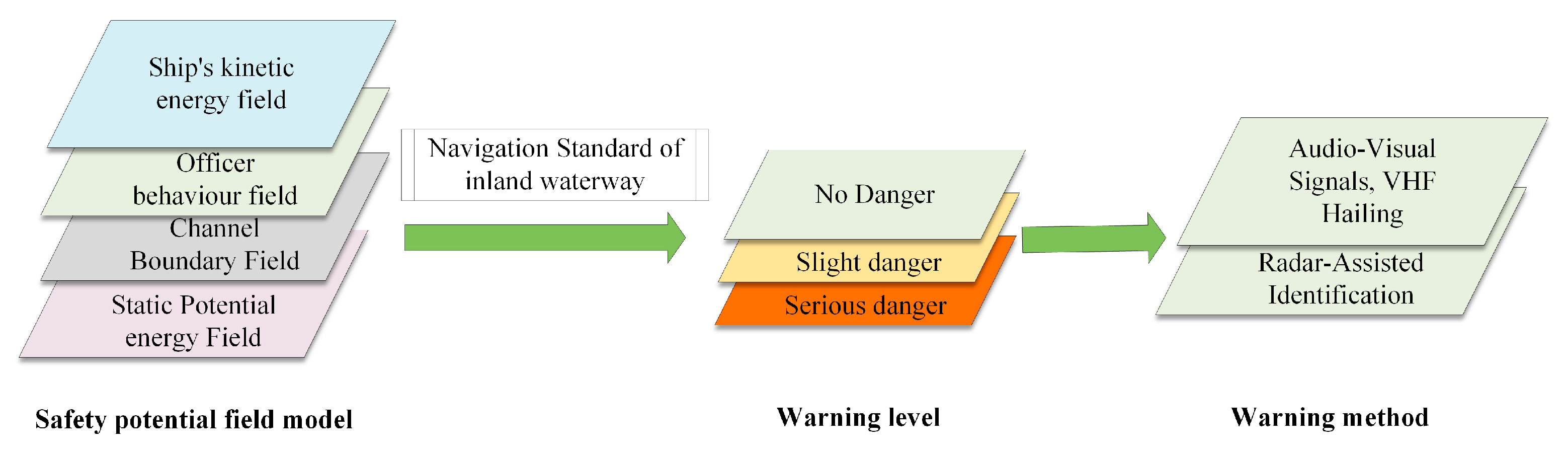
2.2. Ship–Bridge Collision Prevention Warning Framework

There are four main factors affecting the safety of ship navigation in bridge areas: human, ship, environment and management. Human factors mainly include the crew’s driving skills, the negligence of a lookout, etc.; ship-related factors mainly include the ship’s movement status; environmental factors mainly include the channel conditions and external environment; and management factors mainly include the lack of maintenance of waterways and bridges and the inadequacy of emergency plans.

Ships navigating in the bridge area are affected by multiple risk sources, while the interaction between the factors also affects the navigation safety of ships. In inland river navigation, as the management factors are not easy to quantify, the bridge area is considered to be in good management condition for this study, and only the human, ship and environmental risk factors are quantified into specific values. Additionally, the current potential field strength is judged in terms of its safety range by setting the safety thresholds in advance and by assessing whether there is a danger of collision with the bridge.

The safety potential field corresponding to the above factors can be divided into four types: potential field, kinetic field, boundary field, and behavioural field. Static risk elements in the bridge area generate potential fields, moving objects and navigable vessels in the bridge area generate kinetic fields, and the channel bank walls and navigation markers generate boundary fields. Factors affecting the safe behaviour of drivers are considered to be behavioural fields. The specific classifications are shown in

Table 1. Risk elements and corresponding safety fields in the waters of the bridge area.

Bridge Area Risk Element	Elemental Characteristics	Corresponding Safety Potential Field
Navigation officers (persons)	Physical quality	Behavioural field
	Mental quality
	Ship navigation skills
Ship	Ship speed	Kinetic energy field
	Ship navigation direction
Environment	Channel boundary	Boundary energy field Boundary energy field Potential energy field Kinetic energy field Kinetic energy field
	Channel width, depth, etc.
	Bridge piers, stationary ships, quay
	Traffic flow conditions
	Channel floating debris
Management	Damaged or unclear navigational aids	Boundary energy field Behavioural field …
	Emergency plan, team coordination
	…

.

Based on the specific characteristics of the risk elements in bridge-area waters, the bridge area can be divided into corresponding safety fields as a whole. However, in the bridge-area waters, the effects of wind currents and other solid forces on ships cannot be ignored. In order to combine the solid force with the virtual force, this paper applies the Kalman filter algorithm to predict the state of the ship, and the solid force acting on the hull will be corrected to adjust the position, speed and other states of the ship.

The kinetic energy field after correcting the ship state is vectorially superimposed with other safety fields to obtain the total safety potential field. By analysing the spatial distribution pairs of the total safety potential field, the risk of ship collision in the bridge-area waters can be quantitatively assessed, and then early warning can be carried out according to the specific field strength. The framework of this study is shown in Figure 1. In Figure 1, the dashed-line represents the different modules that make up the bridge warning, where blue represents the same warning level, green represents each small module, orange represents an explanation of some of the small modules, and purple represents a highlight in this article.

3. Establishment of Safety Potential Field Model in Bridge Area

3.1. Static Elemental Potential Energy Field

According to the Navigation Standard of Inland Waterway, vessels are required to maintain a certain safety distance when passing through bridge areas in order to avoid a collision with bridge piers and other structures. Therefore, a certain range around bridge piers and other static objects is regarded as an inaccessible area for ships. In order to effectively manage this distance and dynamically assess the interactions between ships and static elements, the concept of the potential energy field is introduced to predict and avoid collision hazards by simulating the distance changes between ships and static objects.

Due to the importance of bridge piers for ship–bridge collision avoidance, this section takes bridge piers as an example by which to introduce the potential energy field. Bridge piers are important structures in the navigation channel, and their physical properties naturally form a fixed static potential energy field. The strength and magnitude of a bridge abutment’s potential energy field depends on its properties, including size, structural strength, and location in the water. The potential energy field of each abutment can be considered an independently existing virtual force field with specific spatial distribution properties. The centre of these potential energy fields is usually located at the geometric centre of the bridge abutment and their influence decreases with increasing distance from the centre. The safety of the waters in the bridge area is jointly determined by a variety of static elements in the channel, among which the bridge piers play a central role in ensuring safety. In addition, other static elements in the bridge area, such as bridge abutments and stationary ships, generate their own potential energy fields. The potential energy fields of these elements, together with those of the bridge abutments, form an integrated safety zone network, providing multiple guarantees for navigation safety. To quantitatively describe the potential energy fields of the static elements in the bridge area, the following mathematical model can be used:

$$E_{Si}(x,y)=k_i\cdot {\left({\displaystyle \frac{d_i}{\left|\overrightarrow{r_d}\right|}}\right)}^n$$

(1)

where $E_{si}\left(x,y\right)$ denotes the magnitude of the field strength of static element $i$ at any coordinate position $\left(x_i,y_i\right)$ in the channel area, with the direction of the field strength coinciding with the direction of the vector, as denoted by $r_d$; $d_i$ is the reference size of static element $i$; n is a positive integer denoting the variation of the potential field strength with distance power; and $k_i$ is a constant related to the properties of the static element i (e.g., size, type, etc.). The specific determination is shown in the following equation:

$$k_i=S\cdot S_i^{\alpha }\cdot T_i^{\beta }\cdot I_i^{\gamma }$$

(2)

where S is a normalization constant used to ensure that the dimensions and range of values of $k_i$ are appropriate, $S_i^{\alpha }$ denotes the dimensions of static element $i$, such as radius or cross-sectional area; $T_i^{\beta }$ denotes the type of static element i, which can be expressed as a categorical variable, with different types of static elements having different values of $T_i$; $I_i^{\gamma }$ denotes the structural strength of static element i, or an indicator of the potential impact of the static element; and $\mathsf{\alpha }$, $\mathsf{\beta }$ and $\mathsf{\gamma }$ are indices which are used to indicate the relative importance of each attribute in terms of its impact on $k_i$. $r_d$ is the position vector from the centre of static element i to any point in the channel area, as shown below:

$$|r_d|=\sqrt{{(x_i-x_o)}^2+{(y_i-y_o)}^2}$$

(3)

where $\left(x_0,y_0\right)$ is the position coordinate of the static marker element $\mathrm{O}$, and $\left(x_i,y_i\right)$ is the position coordinate of any point in the channel. The central region of the potential energy field is located in the geometric centre of the static marker element, and the field strength at the centre tends to be close to infinity, the farther away from the centre of the static marker, the smaller is the value of the potential energy, and, when the value is too small, it can be ignored and is considered that no impact on the bridge abutment will occur. According to the Navigation Standard of Inland Waterway, natural and canalised river water crossing a building axis in the normal direction and with the current flow angle should not be greater than 5°, meaning that the ship and both sides of the bridge abutment between the rich width of the I and V channels can be taken as 0.6 times the width of the track zone, and the VI and VII channels can be taken as 0.5 times the width of the track zone, the rich width of the ship, and the bridge abutment between the rich width, as follows:

$$d={\gamma }_2\times (B_s+L\cdot \sin \alpha )(0.5<{\gamma }_2<0.6)$$

(4)

where $B_S$ is the width of the track zone, usually centred on the ship’s track to either side; L is the length of the ship; $\mathsf{\alpha }$ is the flow pressure angle; the research object is a 70,000-tonne bulk carrier with a length of 90 m; and the shortest safe distance of the ship from the bridge abutment is found to be 8 m. In the text, the target object is considered to be in contact when the distance between the target object and the boundary of the static object markers (the bridge abutment) is 10 m, which is indicated by a red line around the static object markers, i.e., the event of collision against the bridge abutment has taken place. Additionally, a distance greater than 20 m indicates that the ship can pass safely, indicated by an orange line around the static object marker. The 2D and 3D potential energy fields generated by static elements such as piers are shown in Figure 2a,b below.

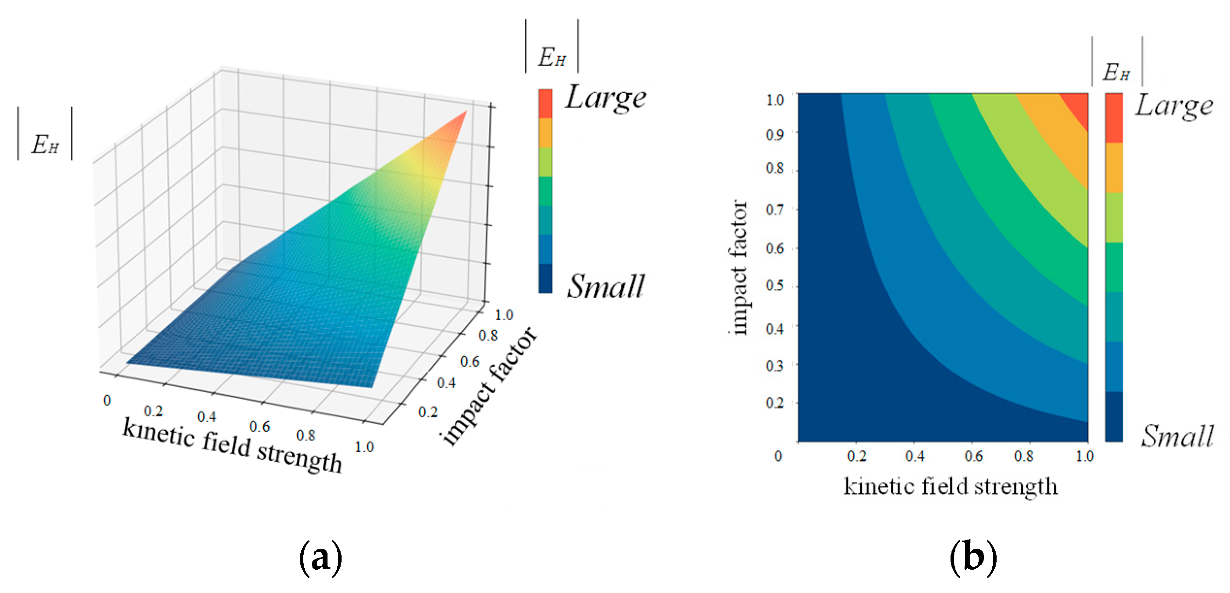
3.2. Dynamic Ship Kinetic Energy Field

In navigating in the bridge area, vessels must maintain the correct vessel position and safe speed to avoid collision with static elements, such as bridge piers. The range and size of the kinetic energy field mainly depend on the motion state of the ship, including the ship speed and turning rate, as well as the nature and distance of the ship. In order to accurately assess the potential hazards of a moving ship, a Gaussian function is used to simulate the kinetic energy field in this study. The kinetic energy field includes not only the kinetic energy of the ship, but also takes into account the effects of its position and speed changes on the environment. The energy field formed by these factors may pose a potential collision threat to the surrounding static structures. Specifically, the mathematical expression for the strength of the kinetic energy field is as follows:

$${{\displaystyle E}}_{Di}=\left\{\begin{array}{ll}\tau \cdot \exp ({\displaystyle \frac{{(v_{kalman}-\mu )}^2}{2{\sigma }^2}})\cdot g\left(\theta ,d_1,d_2\right)\cdot v_{kalman}& v_{kalman}\in \mu \\ K& v_{kalman}\notin \mu \end{array}\right.$$

(5)

where $E_{Di}$ denotes the strength of the kinetic energy vector field at the angle $\theta$ relative to the bridge axis that is normal for the velocity, $v_{kalman}$, predicted by the Kalman filter after considering the effect of the wind flow; $\tau$ is a coefficient to be determined for adjusting the overall strength of the kinetic energy field; and $\mu$ denotes the restricted ship speed in bridge-area waters, which is based on the AIS data of the ships in the vicinity of the Baijusi Bridge after the analysis, which is set to 6–15 knots in this study; $\sigma$ denotes the standard deviation of the velocity distribution; $v_{kalman}$ is the predicted vessel velocity in the bridge area; K is a large constant used to denote the sudden increase in field strength when the velocity exceeds the safe range; the $g\left(\theta ,d_1,d_2\right)$ term reflects the effect of the relative angle between the vessel and the direction normal to the axis of the bridge abutment as well as the vessel’s distance from the abutment, which are explained in the following Equation (6):

$$g\left(\theta ,d_1,d_2\right)=\left\{\begin{array}{ll}0.5\cdot (1+\cos (\theta ))& \theta =0and{d}_1,d_2>\mathsf{\Delta }\\ 2\cdot (1+\cos (\theta ))& \theta =0and\min (d_1,d_2)<\mathsf{\Delta }\\ 1+\cos (\theta )& \mathrm{else}\end{array}\right.$$

(6)

where $d_1,d_2$ denote the distance of the ship from the two bridge abutments and $\Delta$ is the threshold value of the ship’s distance from the bridge abutments set according to the Navigation Standard of Inland Waterway.

By quantifying the potential collision hazard to the static elements in the bridge area when the ship changes its speed and direction due to wind currents and other factors, the hazard can be assessed more accurately. The kinetic energy field of a dynamic ship, for example, is shown in Figure 3a, which displays the effect of speed and angle on the kinetic energy field, and Figure 3b, which displays the strength of the potential field of the ship in a certain area.

3.3. Channel Boundary Potential Field

In inland waterway navigation, the boundary limits imposed by the bank and navigational marking facilities have a higher restraining effect on passing ships compared with the static potential energy field and are intended to warn passing ships of deviations from their normal travelling position and to prevent them from running aground or touching the bank wall. A threshold range for the boundary potential energy field is set to ensure that the ship can navigate within a safe distance. To simplify the representation, the channel can be abstracted as a uniformly extended straight line, with the coordinate axis x direction aligned with the travelling direction of the ship in the channel and the coordinate axis y direction perpendicular to it. Let the target ship A be located at $\mathrm{t}\left(x_i,y_i\right)$, $E_{R1}$ denotes the field strength from the bank wall of the channel and $E_{R2}$ denotes the field strength from the navigational beacon. The boundary field $E_R$, considering the bank wall on both sides of the channel, is thus defined as follows:

$$E_R=E_{R1}+E_{R2}$$

(7)

Of these, the safety potential field effect of the channel bank wall on the ship is as follows:

$$E_{R1}={\displaystyle \sum _{j=1}^2{\mu }_1}exp\left[{({\displaystyle \frac{1}{|r_{aj}|}})}^b\right]$$

(8)

Of these, the influence of the navigational markers on the safety potential field of the ship is as follows:

$$E_{R2}={\displaystyle \sum _{i=1}^2{\mu }_2}exp\left[{({\displaystyle \frac{1}{\left|r_{bi}\right|}})}^b\right]$$

(9)

In the formula, ${\mu }_1$ and ${\mu }_2$ are the coefficients of determination for the boundary field of the channel and the navigational marker, respectively; $r_{aj}$ indicates the vector distance of the target ship A from the shore wall on both sides of the channel, and the lengths are $r_{a1}$ and $r_{a2}$; $r_{bj}$ indicates the vector distance of the target ship $A$ from the navigational mark on both sides, and the lengths are $r_{b1}$ and $r_{b2}$, with the different distances causing a change in the strength of the boundary field; $b$ is the trend of the gradient of the negative correlation of the distance. That is, the closer the ship is to the shore wall and the navigational markers on both sides of the channel, the larger the boundary field is, and the higher the degree of danger; the specific values of $r_{aj}$ and $r_{bj}$ can be obtained from the respective and following provisions of the Navigation Standard of Inland Waterway:

• The safety distance from the outboard side of the cargo ship to the edge of the fairway may be taken as 0.34~0.40 times the width of the track zone, and the safety distance between the outboard side of the ship and the embankment of the fairway, as follows:

  $$r_{aj}={\gamma }_1\times (B_s+L\cdot \sin \alpha )(0.34<{\gamma }_1<0.40)$$

  (10)
• Safe distance between the ship’s outboard side and the navigational markers, as follows:

  $$r_{bj}=1.0\times B_s$$

  (11)
• The boundary field schematic, which is shown in Figure 4.

3.4. Behavioural Fields Based on Crew Behaviour

Bridge-area waters are usually characterised by narrow channels, complex currents and restricted navigational conditions, requiring ships to perform delicate manoeuvres to ensure safe passage. The influence of the driver on the safety of ship navigation is transmitted outward through the ship driven. Therefore, when constructing the behavioural field model, the product of the anthropogenic risk factors and the kinetic energy field formed by the navigating ship can be used to represent the driver’s behavioural field. Through the analysis, the strength of the behavioural field formed by the driver of the target ship $O\left(x_o,y_o\right)$ at its surrounding $i\left(x_i,y_i\right)$ can be expressed as follows:

$$E_{Hi}(x,y)=E_{Di}(x,y)H_r$$

(12)

i.e.:

$$E_{Hi}(x,y)=\left\{\begin{array}{ll}{H}_r\cdot \tau \cdot \exp ({\displaystyle \frac{{(v_{kalman}-\mu )}^2}{2{\sigma }^2}})\cdot g\left(\theta ,d_1,d_2\right)\cdot v_{kalman}& v_{kalman}\in \mu \\ H_r\cdot K& v_{kalman}\notin \mu \end{array}\right.$$

(13)

where $E_{Hi}\left(x,y\right)$ is the behavioural field vector of the driver at $i\left(x,y\right)$, which reacts to the degree of potential danger generated by the driver in the ship’s surroundings under a certain channel condition. The larger the field strength, the greater the potential danger generated by the driver, and the smaller the field strength, the smaller the potential danger generated by the driver; the direction of this behavioural field strength vector is the same as the direction of the ship’s kinetic energy field strength. $H_r$ is the hazard factor affecting the safety of the ship’s officer and includes the crew training, situational awareness, emergency response, skill level and violation of regulations [31]. $v_{kalman}$ is the velocity vector predicted by the Kalman filter, taking into account the influence of wind flow and other factors. The schematic diagram of the behavioural field strength is shown in Figure 5.

3.5. Superposition Field Model

By superimposing Equations (1), (5), (7) and (12), the form of each safety field after superposition, expressed by Equation (14), can be obtained. Using the ship sailing direction as the x-axis and the vertical ship sailing direction as the y-axis, the coordinate system can be established. Figure 6 shows the superimposition field model of the water area in the bridge region, where red represents navigation marks, black squares represent docks, solid and dashed lines represent gridding of the water area, and simple ship icons represent up and down ships. By comprehensively considering the interactions of the potential energy field $E_{Si}$, the kinetic energy field $E_{Di}$, the boundary field $E_R$ and the behavioural field $E_{Hi}$, the superimposed fields provide a comprehensive safety assessment for ships navigating in the bridge area.

$$E_T=E_{Si}(x,y)+E_R(x,y)+E_{Di}(x,y)+E_{Hi}(x,y)$$

(14)

Each field strength describes the potential navigational risk posed by the corresponding type of traffic factor in an actual navigation scenario.

4. Vessel Warning for Bridge Area Based on Vessel Posture

The design of ship–bridge collision warning is based on the established potential energy field of static elements, the kinetic energy field of moving ships, the boundary energy field and the driver behaviour field. Through the grid-based analysis of the waters, the safety conditions in different areas can be accurately assessed, and the superposition effect of each field strength can be explored in order to effectively predict and prevent ship–bridge collision accidents. The specific range and threshold of early warning potential field values are formulated according to the provisions of the Navigation Standard of Inland Waterway on the safe navigation of ships in bridge areas. These values not only consider the interactions between static and dynamic elements, but also integrate the effects of ship movements and pilot behaviour on safety. The warning status is updated in real time according to the preset thresholds and field strength changes, and is classified into no danger, slight danger and severe danger levels. By means of sound and light signals, ship communication, etc., the system provides instant safety prompts and decision-making support to help drivers take timely collision avoidance measures and effectively reduce the risk of collision accidents, thus providing a key guarantee for the safety management of the bridge area. The specific warning process is shown in Figure 7.

The establishment of the safety potential field is based on the theory of virtual forces; however, the influence of solid forces, such as wind currents, cannot be ignored when ships navigate in a bridge area. In order to effectively deal with the effects of these solid forces on ships in terms of bridge collision avoidance, the introduction of Kalman filtering for ship state prediction, while considering wind flow, is necessary. The corrected ship state through Kalman filtering can more accurately reflect the actual bridge conditions, and the predicted state is input into the kinetic energy field model to calculate the overall safety field strength. This is combined with the safety potential field warning method [32] to achieve accurate prediction and effective warning for ships in a bridge area. Figure 8 shows the combination of Kalman filter and safety potential field model.

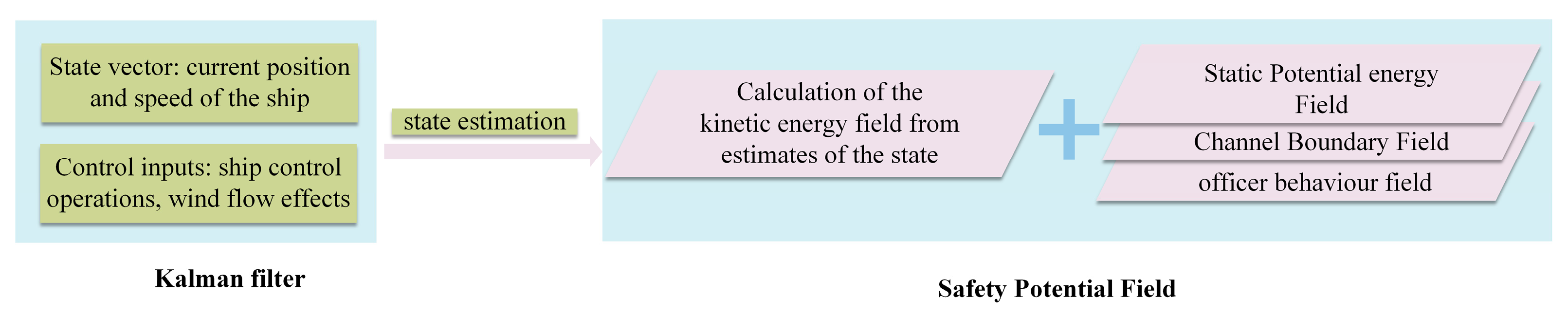
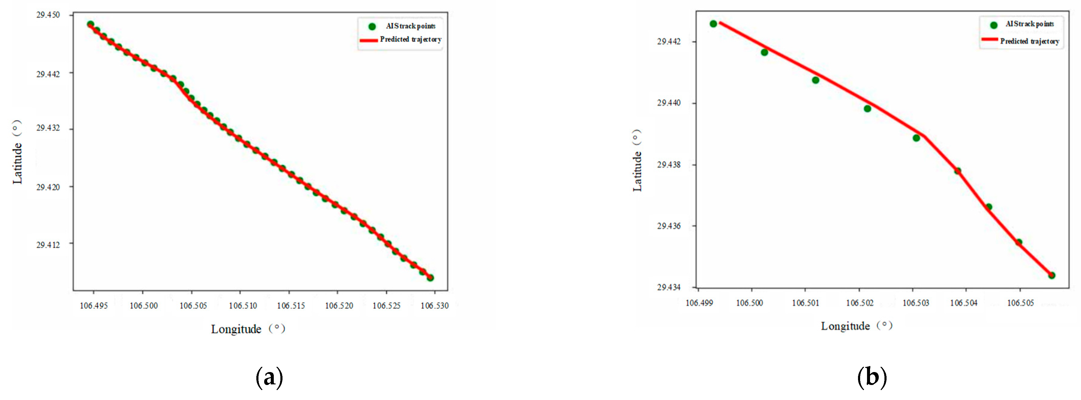
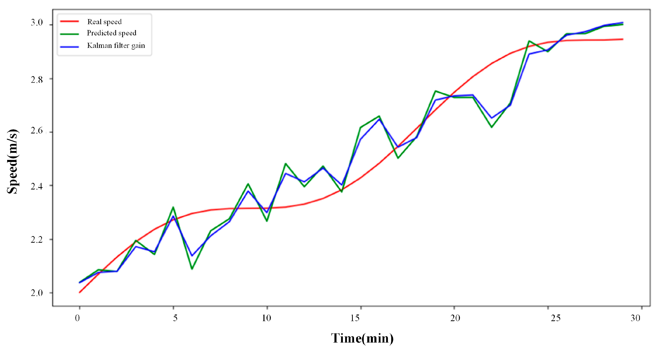
4.1. Ship State Prediction Based on Kalman Filtering

The Kalman filter, based on the state–space model, can effectively estimate the state of dynamic systems [33]. By incorporating historical ship position data and navigation characteristics, and calculating changes at each time step, the Kalman filter can continuously predict ship positions and speeds over a period of time. This method helps to identify potential dangers in a timely manner and take appropriate measures to ensure the safety of navigation in bridge areas. The algorithm uses the minimum mean square error as the optimization criterion and mainly includes two stages—the prediction process and the state update—to achieve optimal estimation of the system’s dynamic state. The system state equation and observation equation are shown as follows:

$$\left\{\begin{array}{l}X(k)=A\times X(k-1)+B\times i(k-1)+CW+w(k-1)\\ Z(k)=H\times X(k)+\psi (k)\end{array}\right.$$

(15)

where $C$ is the wind flow impact matrix and $W$ is the wind flow impact vector; other specific parameters are described in the literature [34].

The prediction of ship trajectory and speed using Kalman filtering is undertaken in the following steps [34]:

• Step 1: Establish the ship motion model and observation model. The transfer function is constructed through physical principles to form the ship motion process model and observation model expressed in state space.
• Step 2: Use the established motion process model and observation model to predict the ship’s state and observation values at the next moment. The ship state quantities (position and speed) at the current moment are taken as inputs, the state at the next moment is estimated by the motion process model, and the observation values at the next moment are obtained by combining the observation model.
• Step 3: Correct the predicted values in step 2 based on the measured values of the ship state acquired by the sensors. The error between the measured value and the predicted value is calculated and the predicted value is corrected by Kalman gain K, including the estimation of the speed.
• Step 4: Repeat steps 2 and 3 to obtain the ship state measurements at each moment by continuous iteration, thereby realising the prediction of the ship trajectory and speed. The computational formulae used in the above steps are as follows:

  $$\left\{\begin{array}{l}{\widehat{x}}_k^{-}=A{\widehat{x}}_k+B{u}_{k-1}\\ P_K^{-}=A{P}_{k-1}{A}^T+Q\\ K_K=P_K^{-}{H}^T{(H{P}_K^{-}{H}^T+R)}^{-1}\\ {\widehat{x}}_k={\widehat{x}}_k^{-}+K_k(Z_k-H{\widehat{x}}_k^{-})\\ P_k=(I-K_{k}H)P_K^{-}\end{array}\right.$$

  (16)

The specific values in equation are given in the literature [35].

The position of the ship in the geodetic coordinate system is represented by the latitude and longitude coordinates $\left(x\left(k\right),y\left(k\right)\right)$. Assuming that the ship’s speed and heading are known, the ship’s latitude and longitude at the moment k can be obtained according to the following equation, based on the constant direction line sailing method, as follows [36]:

$$\left\{\begin{array}{l}x(k)=x(k-1)+V(k-1)T\cos (C(k-1))+W_x(k-1)\\ y(k)=y(k-1)+V(k-1)T\sec (x_m(k-1))\sin (C(k-1))+W_y(k-1)\end{array}\right.$$

(17)

where $x\left(k\right)$ denotes the longitude of the ship at moment k; $V$ denotes the ship’s speed to the ground, i.e., the ship’s speed after considering the effects of wind and current; T denotes the time step of prediction; $C$ denotes the ship’s heading to the ground, i.e., the ship’s heading after considering the effects of wind and current; $y(k$) denotes the ship’s latitude at moment k; $W_x\left(k-1\right)$ denotes the noise of the prediction process for the longitude; $W_y\left(k-1\right)$ denotes the prediction process for the latitude noise, both of which are Gaussian white noise with mean value 0; $X_m\left(k-1\right)$ denotes the average value of latitude at moment $k-1$ and latitude at moment $k$. The calculation formula is shown in (18).

$$X_m(k-1)={\displaystyle \frac{x(k-1)+x(k)}{2}}$$

(18)

By organising Equation (17) into matrix form, the system state equation can be obtained, as follows:

$${[x(k),y(k)]}^T=A{[x(k-1),y(k-1)]}^T+B{i}_{k-1}+Cw+W_{k-1}$$

(19)

where state vector $X\left(K\right)={\left[x\left(k\right),y\left(k\right)\right]}^T$; control input matrix B = ${\left[\begin{array}{cc}T& \begin{array}{ccc}0& T& 0\end{array}\\ 0& \begin{array}{ccc}T& 0& T\end{array}\end{array}\right]}^T$; control input vector $i_{k-1}$=$\left[\begin{array}{c}V\left(k-1\right)cos\left(C\left(K-1\right)\right)\\ V\left(k-1\right)\mathit{sec}\left(x_m\left(k-1\right)\right)sin\left(c\left(k-1\right)\right)\end{array}\right]$; wind flow impact matrix C =${\left[\begin{array}{cc}T& \begin{array}{ccc}0& T& 0\end{array}\\ 0& \begin{array}{ccc}0& T& 0\end{array}\end{array}\right]}^T$; wind flow impact vector $w=\left[\begin{array}{c}{w}_x\left(k-1\right)\\ w_y\left(k-1\right)\end{array}\right]$; and process noise $W_{k-1}=\left[\begin{array}{c}{W}_x\left(k-1\right)\\ W_y\left(k-1\right)\end{array}\right]$. The state transfer matrix A is shown in Equation (20), as follows:

$$A=\left[\begin{array}{cccc}1& 0& T\cos (C(k-1))& 0\\ 0& 1& 0& T\sec (x(k-1)\sin (C(k-1))\\ 0& 0& 1& 0\\ 0& 0& 0& 1\end{array}\right]$$

(20)

Assume that the position of the ship at moment k is ${\left[x\left(k\right),y\left(k\right)\right]}^T$ and the observation noise during the observation is $\psi \left(k\right)$, then the measurement of the system at moment k is as follows:

$$\left\{\begin{array}{l}{z}_x(k)=x(k)+{\psi }_x(k)\\ z_y(k)=y(k)+{\psi }_y(k)\end{array}\right.$$

(21)

By organising Equation (21) in the form of a matrix, the system dynamic measurement equation can be obtained, as follows:

$$Z(k)=AX(k)+\left[\begin{array}{c}{\psi }_x(k)\\ {\psi }_y(k)\end{array}\right]$$

(22)

where observation matrix A is as shown above; $\mathrm{Z}\left(\mathrm{k}\right)={\left[Z_x\left(k\right),Z_y\left(k\right)\right]}^T$; $\psi \left(k\right)=\left[\begin{array}{c}{\psi }_x\left(k\right)\\ {\psi }_y\left(k\right)\end{array}\right]$.

Figure 9a shows the trajectory prediction map of the ship sailing for a period of time, the real trajectory of the ship’s AIS in the figure is represented by green dots, the interval of the dots is 0.5 min, and the red line is the predicted ship’s trajectory. From the figure, it can be seen that the predicted effect of tracking the ship movement nodes is in line with the requirements of ship trajectory prediction and tracking in the waters of the bridge area.

Figure 9b shows the local map of the trajectory prediction of the ship when altering course motion, from which it can be seen that the ship’s trajectory prediction is better when the heading is stable, and that there is a certain degree of error during the ship’s turning process.

Table 2. Comparative analysis of prediction errors between straight and altered course trajectories.

	Pre-Longitude	Pre-Latitude	AIS-Longitude	AIS-Latitude	Error Longitude	Error Latitude
Straight-line navigation	106.503861	29.437757	106.503847	29.4378	0.000014	0.000043
Altering course	106.500388	29.441710	106.50023	29.441663	0.000155	0.000047

shows the trajectory prediction error analysis between the ship’s straight-line navigation and its redirection when the prediction time is set to 0.5 min. The error between the predicted ship position and the AIS-measured ship position is 5.0 m in the case when the ship’s navigation is a straight line, and is 9.8 m the ship alters course. The ship position errors are within the acceptable range.

Figure 10 shows the comparison between the predicted ship speed and the real speed, the green line in the figure is the predicted ship speed, the AIS data point interval is 0.5 min, the red line is the real ship speed, and the blue line is the Kalman filter gain. It can be seen from the figure that the maximum difference between the predicted speed and the real speed is 0.25 m/s, and that the Kalman filter can accurately predict the ship’s movement speed, which can satisfy the requirements of ship trajectory prediction and tracking in the bridge area.

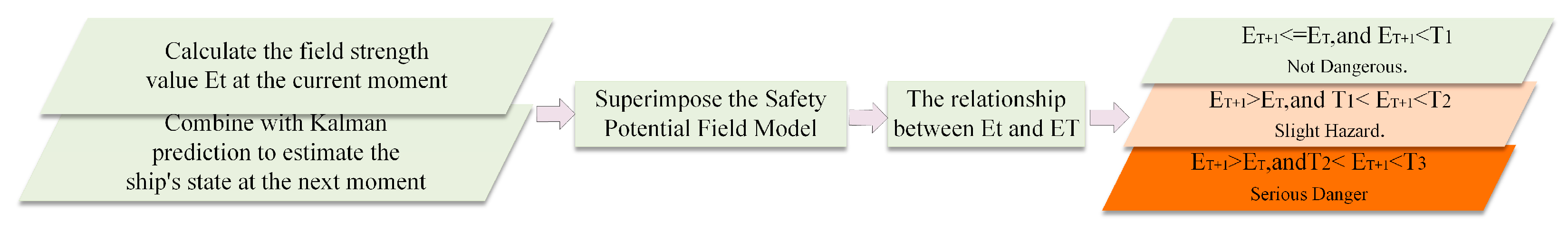
4.2. Real-Time Early Warning Method for the Safety Potential Field of a Bridge Area

The static element potential energy and boundary fields form a fixed field due to their constant position, and can be used to determine the hazardous areas of the bridge area, i.e., areas inaccessible to ships. Through Kalman filtering and safety potential field modelling, the instantaneous integrated field strength value, $E_T$, is calculated, and the integrated field strength $E_{T+1}$ at the next moment is predicted. According to the comparison results of $E_T$ and $E_{T+1}$, the warning is divided into three levels, and different levels correspond to different warning signals, which suggests the possible dangers faced by the ship, so that timely collision avoidance measures can be taken to ensure the safety and effectiveness of navigation in the bridge area. The specific warning levels are as follows:

• $E_{T+1}\le E_T\mathrm{and}{E}_{T+1}\in T_1$: $T_1$ is the safe potential field range of the first level of warning, $E_{T+1}$ is the predicted composite field strength at the next moment, and $E_T$ is the superimposed field strength of the current ship position. If the predicted field strength is less than the current field strength, this indicates that the ship’s navigation in the bridge area is safe and that there is no danger of hitting obstacles such as bridge abutments or the navigation channel. This is part of level 1 and is not dangerous;
• $E_{T+1}>E_T \mathrm{and}{E}_{T+1}\in T_2$:$T_2$ is the potential field range for a level 2 warning. Here, the predicted field strength is stronger than the current field strength, indicating that there is a possibility of the vessel impacting the bridge elements. However, as the predicted field strength is still within the $T_2$ range, this indicates that the current situation in the bridge area has not yet reached the level of urgency and is classified as level 2, or a slight hazard;
• $E_{T+1}>E_T \mathrm{and}{E}_{T+1}\in T_3$:$T_3$ is the potential field range for a level 3 warning. Here, the predicted field strength value continues to increase and is within the range of a level 3 warning, indicating that the ship’s danger to the bridge area is increasing and has reached a degree of urgency that is of the third level, serious danger, as shown in Figure 11.

The steps of the early warning algorithm are as follows:

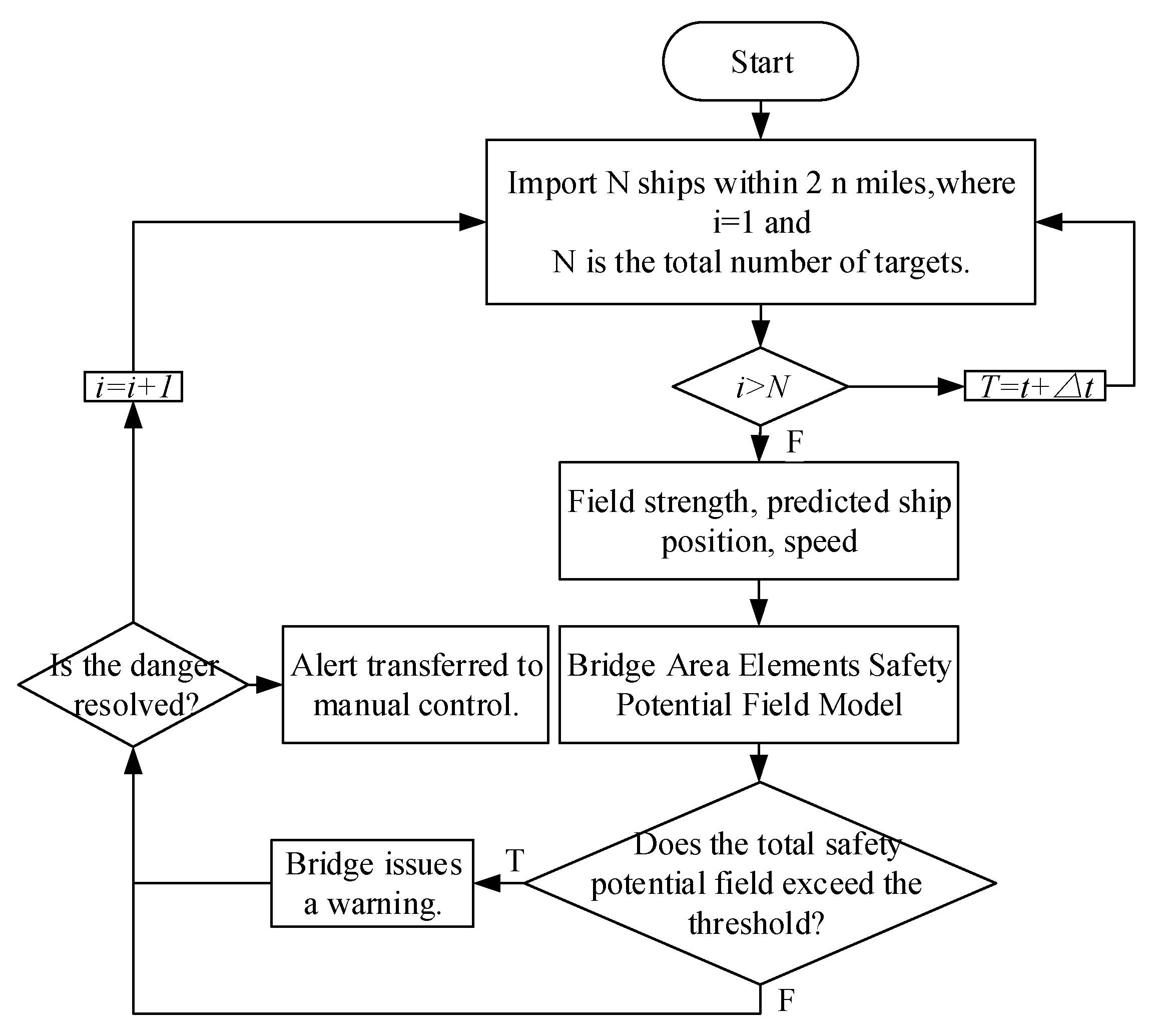
• Step 1: Data collection: collect the environmental data and the real-time dynamic data of ships within 2 nautical miles and number each ship through a VTS, AIS and video monitoring system in the bridge area;
• Step 2: Take out the ship numbered i (i = 1,2,3,…N), calculate the field strength at the current moment based on the ship’s current position information, heading information, and speed information, and predict the ship’s movement position and speed after 2 min;
• Step 3: The predicted position, velocity, and other data are passed into a safe potential field model consisting of bridge zone elements;
• Step 4: Determine whether the integrated safety potential field exceeds the threshold by comprehensively evaluating all potential fields and determining whether the overall safety potential field exceeds the threshold;
• Step 5: Update cycle: As time passes (T = t + ∆t), repeat steps 1 to 5 and continue to judge the next ship i + 1.

Target ships that are too far away from the bridge area can be temporarily disregarded, and ship state prediction is performed only when the target distance is less than the threshold value $D_d$. $D_d$ can be determined by the navigational conditions of the specific waters, with 2 nm taken as the interim value.

In the above steps, by continuously updating the information and predicting the status of the target ship, and by interacting with the bridge area hazardous obstacle model in real time, the safety decision making of ship collision prevention in bridge-area waters can be achieved. These time-series rolling calculations can adapt to the manoeuvring and unpredictable behaviour of the target ship and improve the safety of the bridge-area waters. The specific flow is shown in Figure 12.

5. Simulation Experiments

In this section, the hazards of ship navigation in inland river bridge areas are studied as example. In the case study, a two-way inland waterway is selected and simulated using the safety potential field model proposed in Chapter III. The study is divided into two steps: firstly, the bridge area as a whole at a certain moment is selected as the research scenario, and the superposition field is used to calculate the overall danger of the bridge area environment to obtain the instantaneous potential field strength; secondly, the process of upward and downward vessels crossing the bridge area is taken as the object of the study, and changes in the potential field under the predicted state and the real AIS data are compared and analysed. Based on the calculation results of the safety potential field, the magnitude of the risk distribution in the bridge area under the static scenario and the warning level of ship collision prevention in the bridge area under the dynamic traffic situation are determined.

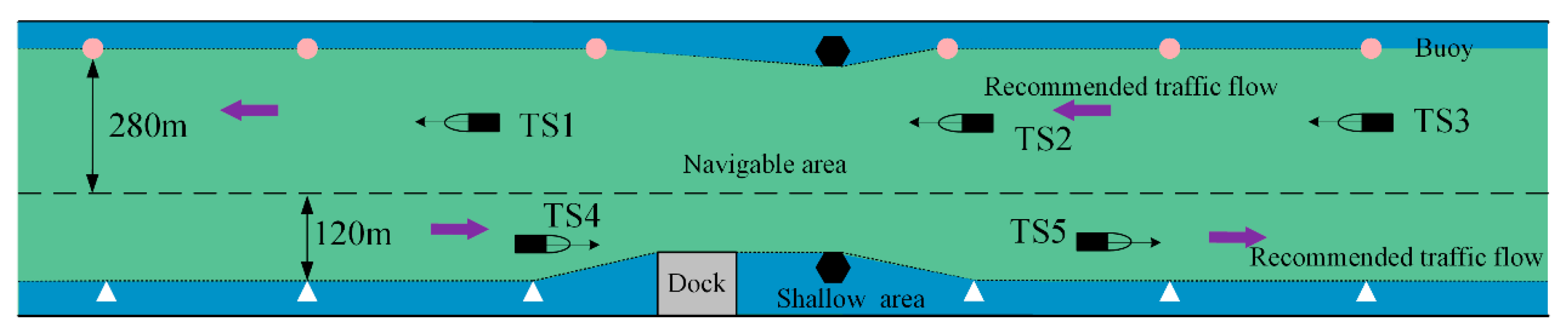
5.1. Experimental Setup

The two-way navigation channel of the Baijusi Bridge in Chongqing is taken as an object, as shown in Figure 13. The total length of the channel is 3000 m, of which the widths of the upstream and downstream channels are 280 m and 120 m, respectively. The average distance from the red buoy to the upper side of the channel is 30 m, and the average distance from the white buoy to the lower side of the channel is 35 m.

In the simulation scenario, the conditions on both sides of the channel are similar and the driving crews have good skills. The coefficients to be determined for the channel boundary field and the coefficients to be determined for the navigational markers are the same, and the influence of the ship driver on the ship in the behavioural field is considered to be constant. The proposed experimental method is validated using ship model parameters in the case study, as shown in

Table 3. The parameters for the safety potential field model used in the case study.

Parameter	Value
${\mathit{k}}_{\mathit{i}}$	2.5
$\mathsf{\tau }$	0.18
$\mathsf{\beta }$	2.2
${\mu }_i$	20
$H_r$	0.1

. The specific procedure of the experiment and the analysis of the related results are described below.

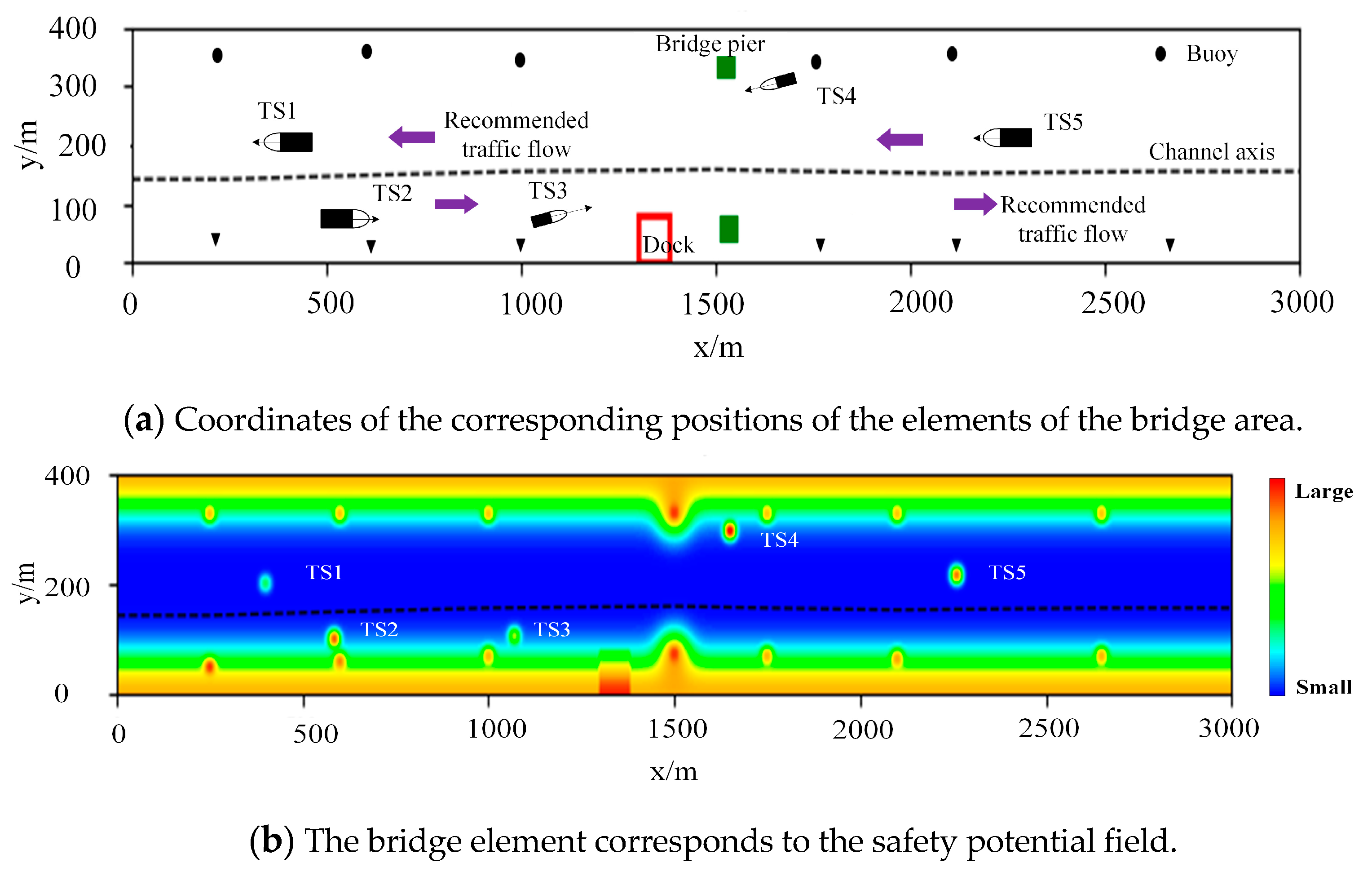
5.2. Bridge Area Safety Potential Field Experiment

According to the experimental setup, based on the superimposed field model, the instantaneous navigation risk generated by each type of element within the bridge area can be calculated and the distribution of the navigational risk in the channel can be represented by a potential field. The study area is gridded and the lateral navigation risk is compared by means of a cross-section perpendicular to the navigation direction in order to determine the location of the risk magnitude in the following cross section. Next, the safety potential fields at the grid points of each longitudinal section of the navigation channel are compared to obtain the distribution of the potential field size of the overall safety field to determine the magnitude of the risk.

Some AIS ship data of Baijusi bridge area on 2 May 2024 are selected, and the relationship between ships and bridge area is shown in Figure 14a. Where TS1, TS2, TS3, TS4 and TS5 represent the ships navigating in the waters of the bridge area, and the ship parameters are shown in

Table 4. Instantaneous channel vessel information.

Ship Number	1	2	3	4	5
Length of ship	110	110	85	85	110
Width of ship	16	16	11	11	16
Speed	8	8	8	8	12
Course	330	150	130	320	320
Distance to piers/m	1100	950	450	150	1000
Distance to ipsilateral navigational markers/m	115	35	35	35	115

. Where the black solid line represents the channel boundary, the dotted line represents the upstream and downstream channel demarcation line, the circle and triangular markers represent the navigation markers, the green rectangle represents the bridge abutment, and the purple arrow represents the direction of traffic flow. According to Chapter 2, the corresponding safety potential field of the bridge area elements established is shown in Figure 14b.

As shown in Figure 14a, TS1 and TS2 are travelling in the channel with the same dimensions, but the risk of TS2 is significantly greater than that of TS1 (as shown in Figure 14b) because TS2 is closer to the edge of the channel, in line with the nautical practice. The distances from the same side of the channel to the navigational markers are the same for both TS1 and TS3, but the risk for TS2 is significantly greater than that for TS3 in Figure 14b because of the larger dimensions of TS2. TS3 and TS4 are the same size in Figure 14a; however, in Figure 14b, TS4 is closer to the bridge abutment, so the risk value for TS4 is significantly greater than that for TS3. In Figure 14a, TS1 and TS5 are the same size and both are upstream sailing vessels; however, in Figure 14b, the risk for TS5 is significantly greater than that for TS1 because the speed of TS5 is significantly faster than that of TS1. The faster the speed, the higher the field strength value.

In summary, different types of ships, or the same type of ship, produce different transient navigation risks due to their different distances from beacons, bridge abutments and piers, or different speeds.

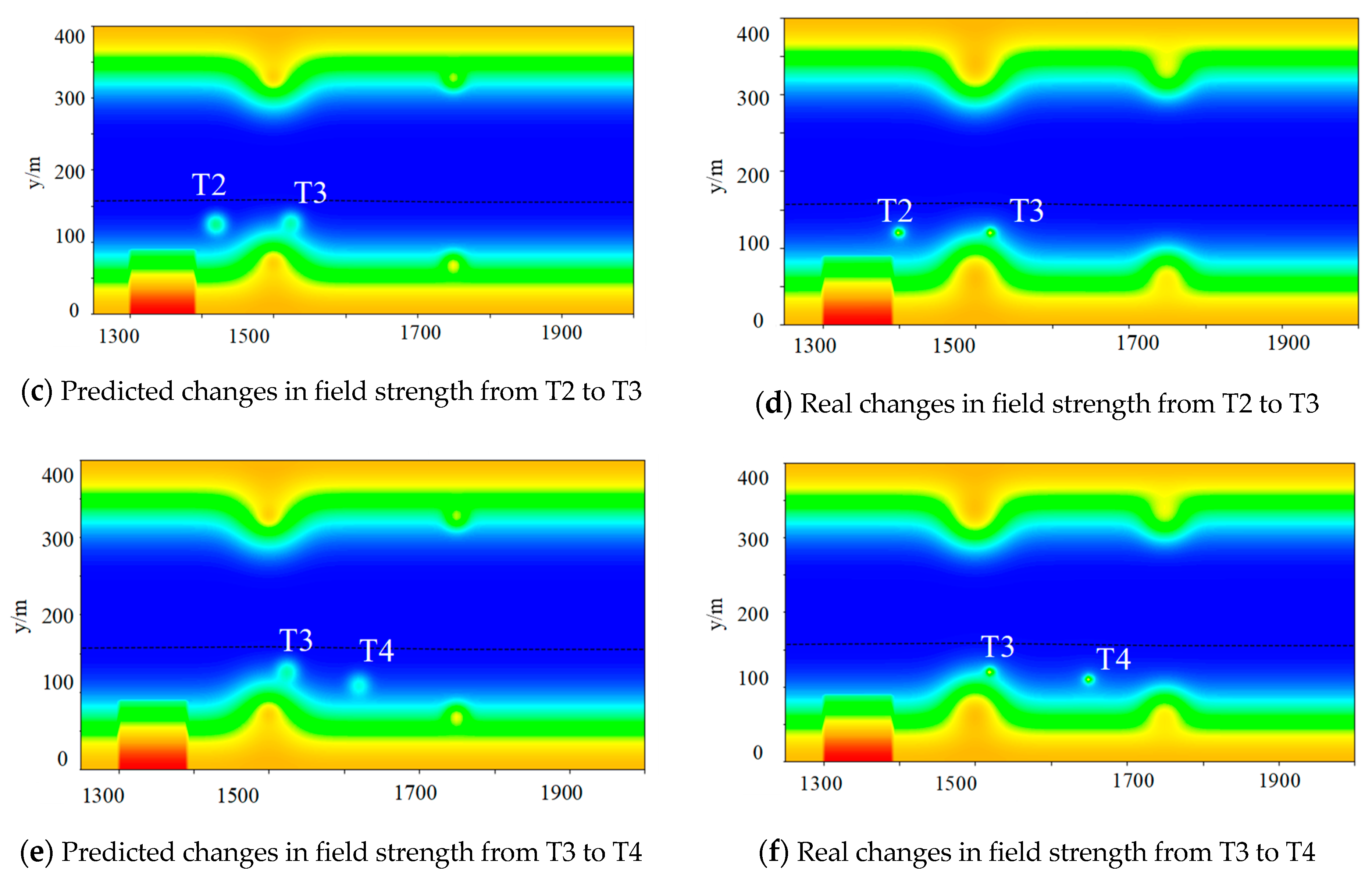
5.3. Bridge Area Early Warning Experiment

In this section, the AIS data of the upstream bulk carrier Shengyuan 506 and the downstream multipurpose ship Shuiyu Huanjing 16, in the bridge area from 10:00 to 13:00 on 5 June 2024, are selected. The state of the two vessels in the bridge area is predicted every 30 s. Using the safety potential field model, the field strength prediction values for the upstream and downstream vessels at different times are calculated. Combining the risk early warning method proposed in Section 3.2, the dynamic changes of the potential field are analysed to determine the risk levels of the vessels and take corresponding early warning measures. Meanwhile, in order to more intuitively illustrate the relationship between field strength values and warning levels, the predicted field strength values and the actual safety potential field values corresponding to the AIS data are normalised so that they are both in the range of 0–1 in order to eliminate the differences in magnitude between the different features and so that the potential field values and the warning ranges can be compared on the same scale.

Taking an upstream bulk carrier as an example, the vessel parameters are shown in

Table 5. Parameters of the upstream bulk carrier.

Parameters	Values
Ship Name	Shengyuan 506
Length	100 m
Width	24 m
Draft	11 m
Speed	10 kn

. The field strength values and early warning levels at four moments during a vessel’s upstream voyage—approaching the edge of the channel, sailing near the bridge abutment, directly in front of the bridge abutment, and passing the bridge abutment—are analysed. The specific early warning level analysis results are shown in

Table 6. Warning levels for different moments of prediction versus real AIS scenarios.

Time Point	Projected Value	Warning Level	AIS Value	Warning Level	Error	Range of Warning Levels
T1	-	Level 1	0.30	Level 1	-	Level 1 (0–0.50)
T2	0.79	Level 2	0.74	Level 2	0.05	Level 2 (0.51–0.80)
T3	0.25	Level 1	0.21	Level 1	0.04	Level 3 (0.81–1)
T4	0.20	Level 1	0.18	Level 1	0.02

.

Figure 15a,b show the predicted and actual instantaneous risks of the vessel from time T1 to T2. At T1, the vessel’s risk value is 0.3, with a warning level of 1. The predicted value for T2 is 0.79, while the actual value is 0.74, both with a warning level of 2, and the error is 0.05. Figure 15c,d display the predicted and actual instantaneous risks of the vessel from time T2 to T3. At T2, the vessel’s risk value is 0.74, with a warning level of 2. The predicted value for T3 is 0.25, while the actual value is 0.21, both with a warning level of 2, and the error is 0.04. Figure 15e,f show the predicted and actual instantaneous risks of the vessel from time T3 to T4. At T3, the vessel’s risk value is 0.21, with a warning level of 1. The predicted value for T4 is 0.20, while the actual value is 0.18, both with a warning level of 1, and the error is 0.02.

Taking a downstream multipurpose cargo ship as an example, the vessel parameters are shown in

Table 7. Parameters of the downstream multipurpose cargo ship.

Parameters	Values
Ship Name	Shuiyu Huanjing 16
Length	48 m
Width	14 m
Draft	7 m
Speed	8 kn

. The analysis focuses on the field strength values and warning levels at four moments during its downstream voyage: approaching the edge of the dock, sailing near the bridge abutment, directly in front of the bridge abutment, and passing the bridge abutment. The specific early warning level analysis results are shown in

Table 8. Forecast and real state warning levels at different moments during the downstream process.

Time Point	Projected Value	Warning Level	AIS Value	Warning Level	Error	Range of Warning Levels
T1	-	Level 1	0.30	Level 1	-	Level 1 (0–0.5)
T2	0.79	Level 2	0.69	Level 2	0.1	Level 2 (0.51–0.80)
T3	0.25	Level 1	0.21	Level 1	0.04	Level 3 (0.81–1)
T4	0.20	Level 1	0.18	Level 1	0.02

.

Figure 16a,b show the predicted and actual instantaneous risks of the vessel from time T1 to T2. At T1, the vessel’s risk value is 0.71, with a warning level of 2. The predicted value for T2 is 0.91, while the actual value is 0.81, both with a warning level of 3, and the error is 0.1. Figure 16c,d display the predicted and actual instantaneous risks of the vessel from time T2 to T3. At T2, the vessel’s risk value is 0.81, with a warning level of 3. The predicted value for T3 is 0.45, while the actual value is 0.40, both with a warning level of 1, and the error is 0.05. Figure 16e,f show the predicted and actual instantaneous risks of the vessel from time T3 to T4. At T3, the vessel’s risk value is 0.40, with a warning level of 1. The predicted value for T4 is 0.25, while the actual value is 0.21, both with a warning level of 1, and the error is 0.04.

In summary, it can be seen through the above experiments that there is an error between the prediction results and the AIS calculation results, and the maximum error of 0.1 occurs when the downstream ship passes the pier. At this time, the ship needs to consider not only the distance to the pier, but also the distance to the bridge abutment, so that the predicted value is slightly larger. However, there is no error in the predicted risk level. The predicted field strength potential energy values are generally higher than those calculated by the actual AIS, but both the predicted and true values are within the warning range, which avoids false alarms due to the use of the method. In addition, from a security point of view, the slightly higher predicted values than the actual values are more favourable for drawing attention to the situation.

6. Discussion

This paper focuses on the problem of ship collision avoidance and risk warning in inland river bridge areas. The established safety potential field model can be used for the dynamic simulation of inland river bridge area. The risk assessment of ship navigation in bridge-area waters can facilitate the management of ships in the bridge area and the delineation of virtual hazardous areas, which is conducive to emergency planning [37]. Meanwhile, this helps to assess the safe speed and distance of vessels in complex bridge area environments [38] and improve water traffic management [39,40].

Compared with the existing research on collision warnings for ships and bridges in inland bridge areas, the main innovation of this paper is the overall analysis of collision warning for inland ships and bridges in static and dynamic traffic scenarios based on navigational risk using the safety potential field method. Firstly, the safety potential field model proposed in this paper is different from the previous models [41]. The kinetic field model in this study combines the effects of wind and current when ships navigate in the bridge area. The state of the ship after being subjected to wind and current is predicted by Kalman filtering and the predicted values are used to calculate the kinetic energy field, which is then coupled into the safety potential field model, which is not covered in previous studies. By updating the kinetic energy field at each step, the safety potential field values are also updated, which makes the model more realistic and accurately reflects the changes of the risk in the bridge area. Secondly, this paper applies a risk study to inland ship navigation, which is different from many previous bridge area warning methods [42]. Compared with the radar detection method and with video surveillance and image processing methods, the warning range of the safety potential field-based ship–bridge warning method proposed in this paper includes the entire bridge area, which is broad and computationally small, and can be updated in real time. In addition, the model uses a three-dimensional isopotential map, which can visualise the risk status of the bridge area.

The proposed model can be used for bridge collision avoidance in inland rivers. In terms of risk warning, the model can be used as an early warning system for navigational risks. In addition, the model can improve the management of navigation traffic in the vicinity of bridge areas [7]. For example, the safe distance between inland waterway vessels and the channel bank wall can be quantified and regulated using the proposed model. For bridges, the model can be integrated with shipboard systems or shore-based control systems to guide ships in inland waterways.

7. Conclusions

This paper proposes a collision avoidance method for ships in inland river bridge areas based on the safety potential field theory. This method assesses various risk factors affecting ship–bridge collision prevention and provides real-time warnings. By integrating Kalman filtering with the safety potential field, the method combines physical and virtual forces in the bridge area to predict the next change in field strength for early warning. The risks associated with each element are classified into four categories: static potential fields, dynamic kinetic fields, channel boundary fields, and behavioural fields based on human behaviour. Different potential field functions are established in the model and coupled into the superimposed fields. The method is applied to a case study by simulating the model with a grid of the bridge-area water and analysing the transient risk in the area through the superimposed fields in order to derive the transient hazardous situation of ships navigating in the bridge area. By combining the predicted ship states using Kalman filtering, the overall superimposed field strength of the bridge area at the next moment is obtained. Early warnings are issued by comparing the predicted field strength values at different moments and validating these predictions against the field strength calculated from real-time AIS data to ensure warning accuracy.

The main contributions of this paper are as follows: Firstly, a new collision warning method for bridge protection is proposed, one which analyses the potential causes of ship–bridge collisions from a holistic perspective. Secondly, the factors that may lead to ship collisions in the bridge area are quantified so that the specific risk value of each influencing factor is clearly visible, thus providing bridge monitors with specific risk indicators. Finally, the ship state predicted by the Kalman filter is combined with the potential field to achieve the fusion of virtual and physical forces, which provides theoretical guidance for further research on collision prevention between ships and bridges. In future research, the proposed model should take more factors into consideration, such as the crew’s driving state during navigation, the effect of inertia when the ship is turning or passing through a curved channel, and the method of ship–bridge early warning in special scenarios such as at sea and in curved river sections. In the future, this can be combined with a ship manoeuvring motion model, a neural network and other methods to achieve high-precision ship position prediction and further improve the accuracy of the warning.

References

1. Review of Maritime Transport 2019 | UNCTAD. Available online: https://unctad.org/publication/review-maritime-transport-2019 (accessed on 16 July 2024).
2. van Westrenen, F.; Baldauf, M. Improving Conflicts Detection in Maritime Traffic: Case Studies on the Effect of Traffic Complexity on Ship Collisions. Proc. Inst. Mech. Eng. Part M J. Eng. Marit. Environ. 2020, 234, 209–222. [Google Scholar] [CrossRef]
3. Yu, Y.; Chen, L.; Shu, Y.; Zhu, W. Evaluation Model and Management Strategy for Reducing Pollution Caused by Ship Collision in Coastal Waters. Ocean Coast. Manag. 2021, 203, 105446. [Google Scholar] [CrossRef]
4. Ma, W.; Zhu, Y.; Grifoll, M.; Liu, G.; Zheng, P. Evaluation of the Effectiveness of Active and Passive Safety Measures in Preventing Ship–Bridge Collision. Sensors 2022, 22, 2857. [Google Scholar] [CrossRef]
5. Zhang, W.Z.; Pan, J.; Sanchez, J.C.; Li, X.B.; Xu, M.C. Review on the Protective Technologies of Bridge against Vessel Collision. Thin-Walled Struct. 2024, 201, 112013. [Google Scholar] [CrossRef]
6. AASHTO: Commentary for Vessel Collision Design of Highway Bridges. Available online: https://scholar.google.com/scholar_lookup?title=Guide%20Specifications%20and%20Commentary%20for%20Vessel%20Collision%20Design%20of%20Highway%20Bridges&author=AASHTO&publication_year=2009 (accessed on 17 July 2024).
7. Chen, W.; Wang, Y.G.; Li, W.; Yang, L.M.; Liu, J.; Dong, X.L.; Zhu, H.H.; Wang, F. An Adaptive Arresting Vessel Device for Protecting Bridges over Non-Navigable Water against Vessel Collision. Eng. Struct. 2021, 237, 112145. [Google Scholar] [CrossRef]
8. Fan, W.; Yuan, W.; Chen, B. Steel Fender Limitations and Improvements for Bridge Protection in Ship Collisions. J. Bridge Eng. 2015, 20, 06015004. [Google Scholar] [CrossRef]
9. Xie, R.; Fan, W.; He, Y.; Liu, B.; Shao, X. Crushing Behavior and Protective Performance of Varying Cores in UHPFRC-Steel-Foam Sandwich Structures: Experiment, Optimal Selection and Application. Thin-Walled Struct. 2022, 172, 108886. [Google Scholar] [CrossRef]
10. Wang, Y.; Zhang, R.; Liu, S.; Zhai, X.; Zhi, X. Energy Absorption Behaviour of an Aluminium Foam-Filled Circular-Triangular Nested Tube Energy Absorber under Impact Loading. Structures 2021, 34, 95–104. [Google Scholar] [CrossRef]
11. Zhu, G.; Zhao, Z.; Hu, P.; Luo, G.; Zhao, X.; Yu, Q. On Energy-Absorbing Mechanisms and Structural Crashworthiness of Laterally Crushed Thin-Walled Structures Filled with Aluminum Foam and CFRP Skeleton. Thin-Walled Struct. 2021, 160, 107390. [Google Scholar] [CrossRef]
12. Zhu, L.; Liu, W.; Fang, H.; Chen, J.; Zhuang, Y.; Han, J. Design and Simulation of Innovative Foam-Filled Lattice Composite Bumper System for Bridge Protection in Ship Collisions. Compos. Part B Eng. 2019, 157, 24–35. [Google Scholar] [CrossRef]
13. Wang, J.J.; Song, Y.C.; Wang, W.; Chen, C.J. Evaluation of Flexible Floating Anti-Collision Device Subjected to Ship Impact Using Finite-Element Method. Ocean Eng. 2019, 178, 321–330. [Google Scholar] [CrossRef]
14. Ge, J.; Luo, T.; Qiu, J. Discretized Macro-Element Method to Evaluate the Crushing Behavior and Protective Performance of Crashworthy Devices under Ship Collisions. Ocean Eng. 2024, 306, 118125. [Google Scholar] [CrossRef]
15. Gholipour, G.; Zhang, C.; Mousavi, A.A. Nonlinear Numerical Analysis and Progressive Damage Assessment of a Cable-Stayed Bridge Pier Subjected to Ship Collision. Mar. Struct. 2020, 69, 102662. [Google Scholar] [CrossRef]
16. Pan, J.; Wang, Y.; Xu, M.C. Impact Scenario Models of Ship-Bridge Collision Based on AIS Data. In Proceedings of the 28th International Ocean and Polar Engineering Conference, Sapporo, Japan, 10–15 June 2018; Available online: https://scholar.google.com/scholar_lookup?title=Impact%20scenario%20models%20of%20ship-bridge%20collision%20based%20on%20AIS%20data&publication_year=2018&author=J.%20Pan&author=Y.%20Wang&author=M.%20Xu (accessed on 18 July 2024).
17. Zhang, L.; Chen, P.; Li, M.; Chen, L.; Mou, J. A Data-Driven Approach for Ship-Bridge Collision Candidate Detection in Bridge Waterway. Ocean Eng. 2022, 266, 113137. [Google Scholar] [CrossRef]
18. Wang, X.; Zheng, Z.; You, J.; Qin, Y.; Xia, W.; Zhou, Y. BOPVis: Bridge Monitoring Data Visualization for Operational Performance Mining. Appl. Sci. 2024, 14, 6615. [Google Scholar] [CrossRef]
19. Perera, L.P.; Guedes Soares, C. Collision Risk Detection and Quantification in Ship Navigation with Integrated Bridge Systems. Ocean Eng. 2015, 109, 344–354. [Google Scholar] [CrossRef]
20. Frangopol, D.M.; Dong, Y.; Sabatino, S. Bridge Life-Cycle Performance and Cost: Analysis, Prediction, Optimisation and Decision-Making. In Structures and Infrastructure Systems; Routledge: London, UK, 2017. [Google Scholar]
21. Larsen, O.D. Ship Collision with Bridges: The Interaction between Vessel Traffic and Bridge Structures; IABSE: Zurich, Switzerland, 1993; Volume 4. [Google Scholar]
22. Hörteborn, A.; Ringsberg, J.W. A Method for Risk Analysis of Ship Collisions with Stationary Infrastructure Using AIS Data and a Ship Manoeuvring Simulator. Ocean Eng. 2021, 235, 109396. [Google Scholar] [CrossRef]
23. Liu, Z.; Zhang, B.; Zhang, M.; Wang, H.; Fu, X. A Quantitative Method for the Analysis of Ship Collision Risk Using AIS Data. Ocean Eng. 2023, 272, 113906. [Google Scholar] [CrossRef]
24. Liu, Y.; Guo, X. Study on Risk of Ship Collision in Bridge Life-Cycle Based on Synergetic Theory. Ocean Eng. 2023, 289, 116148. [Google Scholar] [CrossRef]
25. Chen, P.; Huang, Y.; Mou, J.; van Gelder, P.H.A.J.M. Probabilistic Risk Analysis for Ship-Ship Collision: State-of-the-Art. Saf. Sci. 2019, 117, 108–122. [Google Scholar] [CrossRef]
26. Aydin, M.; Akyuz, E.; Turan, O.; Arslan, O. Validation of Risk Analysis for Ship Collision in Narrow Waters by Using Fuzzy Bayesian Networks Approach. Ocean Eng. 2021, 231, 108973. [Google Scholar] [CrossRef]
27. Wu, B.; Yip, T.L.; Yan, X.; Guedes Soares, C. Fuzzy Logic Based Approach for Ship-Bridge Collision Alert System. Ocean Eng. 2019, 187, 106152. [Google Scholar] [CrossRef]
28. Wan, Y.; Liu, C.; Qiao, W. An Safety Assessment Model of Ship Collision Based on Bayesian Network. In Proceedings of the 2019 European Navigation Conference (ENC), Warsaw, Poland, 9–12 April 2019; pp. 1–4. [Google Scholar]
29. Wang, Z.; Wang, W.; Mu, K.; Fan, S. Time-Delay Following Model for Connected and Automated Vehicles Considering Multiple Vehicle Safety Potential Fields. Appl. Sci. 2024, 14, 6735. [Google Scholar] [CrossRef]
30. Goerlandt, F.; Montewka, J. Maritime Transportation Risk Analysis: Review and Analysis in Light of Some Foundational Issues. Reliab. Eng. Syst. Saf. 2015, 138, 115–134. [Google Scholar] [CrossRef]
31. Hetherington, C.; Flin, R.; Mearns, K. Safety in Shipping: The Human Element. J. Safety Res. 2006, 37, 401–411. [Google Scholar] [CrossRef]
32. Li, L.; Gan, J.; Yi, Z.; Qu, X.; Ran, B. Risk Perception and the Warning Strategy Based on Safety Potential Field Theory. Accid. Anal. Prev. 2020, 148, 105805. [Google Scholar] [CrossRef]
33. Fan, Y.; Qiao, S.; Wang, G.; Chen, S.; Zhang, H. A Modified Adaptive Kalman Filtering Method for Maneuvering Target Tracking of Unmanned Surface Vehicles. Ocean Eng. 2022, 266, 112890. [Google Scholar] [CrossRef]
34. Faragher, R. Understanding the Basis of the Kalman Filter Via a Simple and Intuitive Derivation [Lecture Notes]. IEEE Signal Process. Mag. 2012, 29, 128–132. [Google Scholar] [CrossRef]
35. Welch, G.F. Kalman Filter. In Computer Vision: A Reference Guide; Ikeuchi, K., Ed.; Springer International Publishing: Cham, Switzerland, 2021; pp. 721–723. ISBN 978-3-030-63416-2. [Google Scholar]
36. Ristic, B.; La Scala, B.; Morelande, M.; Gordon, N. Statistical Analysis of Motion Patterns in AIS Data: Anomaly Detection and Motion Prediction. In Proceedings of the 2008 11th International Conference on Information Fusion, Cologne, Germany, 30 June–3 July 2008; pp. 1–7. [Google Scholar]
37. Zhang, W.; Feng, X.; Goerlandt, F.; Liu, Q. Towards a Convolutional Neural Network Model for Classifying Regional Ship Collision Risk Levels for Waterway Risk Analysis. Reliab. Eng. Syst. Saf. 2020, 204, 107127. [Google Scholar] [CrossRef]
38. Shu, Y.; Daamen, W.; Ligteringen, H.; Wang, M.; Hoogendoorn, S. Calibration and Validation for the Vessel Maneuvering Prediction (VMP) Model Using AIS Data of Vessel Encounters. Ocean Eng. 2018, 169, 529–538. [Google Scholar] [CrossRef]
39. Xue, J.; Papadimitriou, E.; Reniers, G.; Wu, C.; Jiang, D.; van Gelder, P.H.A.J.M. A Comprehensive Statistical Investigation Framework for Characteristics and Causes Analysis of Ship Accidents: A Case Study in the Fluctuating Backwater Area of Three Gorges Reservoir Region. Ocean Eng. 2021, 229, 108981. [Google Scholar] [CrossRef]
40. Zhang, M.; Zhang, D.; Fu, S.; Kujala, P.; Hirdaris, S. A Predictive Analytics Method for Maritime Traffic Flow Complexity Estimation in Inland Waterways. Reliab. Eng. Syst. Saf. 2022, 220, 108317. [Google Scholar] [CrossRef]
41. Gan, L.; Yan, Z.; Zhang, L.; Liu, K.; Zheng, Y.; Zhou, C.; Shu, Y. Ship Path Planning Based on Safety Potential Field in Inland Rivers. Ocean Eng. 2022, 260, 111928. [Google Scholar] [CrossRef]
42. Bačkalov, I. Safety of Autonomous Inland Vessels: An Analysis of Regulatory Barriers in the Present Technical Standards in Europe. Saf. Sci. 2020, 128, 104763. [Google Scholar] [CrossRef]
Figure 1. Safety potential field model-based ship–bridge collision warning framework.
Applsci 14 09089 g001
Figure 2. Example of static element potential energy field intensity.
Applsci 14 09089 g002
Figure 3. Schematic diagram of the kinetic energy field strength of the dynamic object marker.
Applsci 14 09089 g003
Figure 4. Schematic diagram of the channel boundary model. (a) Schematic diagram of the channel environment boundary model. (b) Example of uniform channel boundary field intensity.
Applsci 14 09089 g004
Figure 5. Schematic diagram of the behavioural field. (a) Variation in the spatial relationship between kinetic energy field strength and influence factors. (b) Variation of kinetic energy field strength in relation to the plane of influence factor.
Applsci 14 09089 g005
Figure 6. Superposition field in the bridge area.
Applsci 14 09089 g006
Figure 7. Warning process based on safety potential field.
Applsci 14 09089 g007
Figure 8. Schematic of the combination of state prediction and security potential field.
Applsci 14 09089 g008
Figure 9. Ship trajectory prediction forecast. (a) Prediction diagram of ship motion when altering course. (b) Local prediction diagram of ship motion when altering course.
Applsci 14 09089 g009
Figure 10. Comparison between predicted and true speed of the vessel.
Applsci 14 09089 g010
Figure 11. Hierarchical warning based on safety potential field.
Applsci 14 09089 g011
Figure 12. Flowchart of a bridge-area safety potential field and ship collision warning.
Applsci 14 09089 g012
Figure 13. Simulated waterway environment diagram.
Applsci 14 09089 g013
Figure 14. Distribution of instantaneous navigational hazards in the bridge area for static scenarios.
Applsci 14 09089 g014
Figure 15. Comparison of channel risk warnings at different moments for cargo ship.
Applsci 14 09089 g015
Figure 16. Comparison of risk warnings at different moments for multipurpose ship.
Applsci 14 09089 g016aApplsci 14 09089 g016b