Article

A Microscopic On-Ramp Model Based on Macroscopic Network Flows

1
Institute of Geometry and Practical Mathematics, RWTH Aachen University, 52062 Aachen, Germany
2
Institute of Highway Engineering, RWTH Aachen University, 52062 Aachen, Germany
3
Federal Highway Research Institute, 51427 Bergisch Gladbach, Germany
*
Author to whom correspondence should be addressed.
These authors contributed equally to this work.
Appl. Sci. 2024, 14(19), 9111; https://doi.org/10.3390/app14199111
Submission received: 22 August 2024 / Revised: 19 September 2024 / Accepted: 4 October 2024 / Published: 9 October 2024
(This article belongs to the Section Transportation and Future Mobility)

Abstract

:
While macroscopic traffic flow models adopt a fluid dynamic description of traffic, microscopic traffic flow models describe the dynamics of individual vehicles. Capturing macroscopic traffic phenomena accurately remains a challenge for microscopic models, especially in complex road sections. Based on a macroscopic network flow model calibrated to real traffic data and new rules for the acceleration and merging behavior on the on-ramp, we propose a microscopic model for on-ramps. To evaluate the performance of the new flow-based model, we conduct traffic simulations assessing speeds, accelerations, lane change positions, and risky behavior. Our results show that, although the proposed model exhibits some limitations, its performance is superior to the Intelligent Driver Model in the evaluated aspects. While the Intelligent Driver Model simulations are almost free of conflicts, the proposed model evokes a realistic amount and severity of conflicts and therefore can be considered for safety analysis.

1. Introduction

Traffic flow models have a wide variety of applications such as transportation planning, traffic management, and road safety analysis; see, e.g., [1,2,3]. Depending on the application, traffic flow can be modeled at the macroscopic and the microscopic scale. Macroscopic models depict aggregated quantities, including traffic flow, traffic density, and mean speed. A description in terms of a scalar conservation law for the vehicle density combined with a concave velocity function (fundamental diagram) has been introduced in the 1950s in seminal works [4,5,6]. Since then, various model refinements have been considered. A prominent one, which extends the single equation approach using another conservation law allowing for more general velocity profiles is the second-order model by [4,7]. These refined models are capable of accurately capturing traffic dynamics on highway sections, as verified in various studies with real world data; see, e.g., [8,9,10]. Network modeling to account for complex geometries such as junctions has also been of mathematical interest in the last decades; see, e.g., [11,12]. Various efficient numerical schemes for such networked systems have recently been developed [13,14]. However, only a few studies have considered the data validation of these network models. Only recently, a macroscopic model for on-ramps based on real data collected on a German highway section in road work zones has been proposed in [15].
Microscopic models, on the other hand, describe the behavior of individual vehicles [16,17,18]. While macroscopic models predict the traffic flow in a large road network more efficiently, microscopic models are required for studying traffic flow in detail in specific traffic scenarios involving, for example, complex geometries [19,20,21]. In these models, the dynamics are typically divided into a longitudinal component, which is described by a car-following model, and a lateral component, which is described by a lane change model. Lateral movements within the lane are usually neglected. There have been numerous car-following models with different underlying concepts proposed in the literature. The Optimal Velocity Model [16] states that drivers aim for an optimal velocity depending on the distance to the leading vehicle. The Full Velocity Difference Model (FVDM) [17] additionally includes speed differences between leading and following vehicles. The Intelligent Driver Model (IDM) [18] distinguishes three driving situations (accelerating, following with constant time headway, and decelerating) and smooth transitions between them. Despite being introduced more than 20 years ago, the IDM is still widely used and performs better than other car-following models in practice [22].
Both the macroscopic and the microscopic modeling approach have their limitations. Macroscopic models make simplifying assumptions; for example, they neglect variability with respect to acceleration [23,24]. Microscopic models describe the dynamics of vehicles in individual detail, but they do not necessarily reproduce empirical macroscopic traffic patterns such as the capacity drop [25]. Under simplifying assumptions, macroscopic traffic models can be derived as an infinite (vehicle) limit of microscopic models; see, e.g., [26]. Consistency of the FVDM model to a macroscopic model in two space dimensions has been mathematically shown and empirically verified [27,28]. A promising approach to combine the advantages of models of both scales is to infer information from macroscopic models into the microscopic models by converting traffic flow into time headways and traffic density into spacings.
The validation of traffic models is usually considered on the macroscopic level and addresses questions such as the following: does the model produce the traffic flow and density expected from real data? Moreover, it is necessary that microscopic models describe driver behavior on the microscopic scale accurately. Different metrics are required to account for the different scales of the models.
To use traffic flow models for road safety analysis, the models must be able to predict the number of accidents or conflicts on a given road section or network [2,29]. While some microscopic models consider driver conflicts, they are mostly built to be accident free, which means vehicles will behave such that accidents cannot happen while simulating traffic [30]. Risky behavior can be captured with so-called surrogate safety measures (SSMs), which quantify the risk of a collision between two interacting vehicles [31] that is possibly averaged over time or space [32]. If vehicles interact, the closer they are to a collision, the less time they have to react. Therefore, more extreme maneuvers are required to avoid a crash. The spatial distribution and severity of these risky interactions can be useful criteria to evaluate the model performance in terms of safety [33]. A model that resembles real traffic in terms of safety makes it possible to evaluate different road designs in the planning phase, which contributes to safer road infrastructure.
In this paper, we derive a new microscopic car-following model for on-ramps based on the macroscopic model proposed in [15], and we discuss the additional requirements on the microscopic scale. Compared to established microscopic lane merging models based on simple rules, the developed approach allows us to better calibrate the model behavior at the junction of available data. Thus, we aim to combine the advantages of the macroscopic and the microscopic scale to obtain a more accurate representation of traffic at on-ramps in terms of traffic flow and safety. Furthermore, we validate the proposed model using real trajectory data in terms of speeds, accelerations, the distribution of lane changes, and the severity of interactions. The predictions are compared with the IDM in combination with a standard lane change model. Figure 1 gives an overview of the modeling, validation, and simulation technique considered in this work.
The rest of this paper is organized as follows: In the Methods section, we first describe our data, the data-driven macroscopic junction modeling approach, and our new approach transferring these principles to microscopic models. We then give details on the implementation and the metrics we use for the model evaluation in the same section. In the Results and Discussion sections, we compare real traffic data at an on-ramp to simulation results obtained by an established microscopic model and our new flow-based approach.

2. Methods

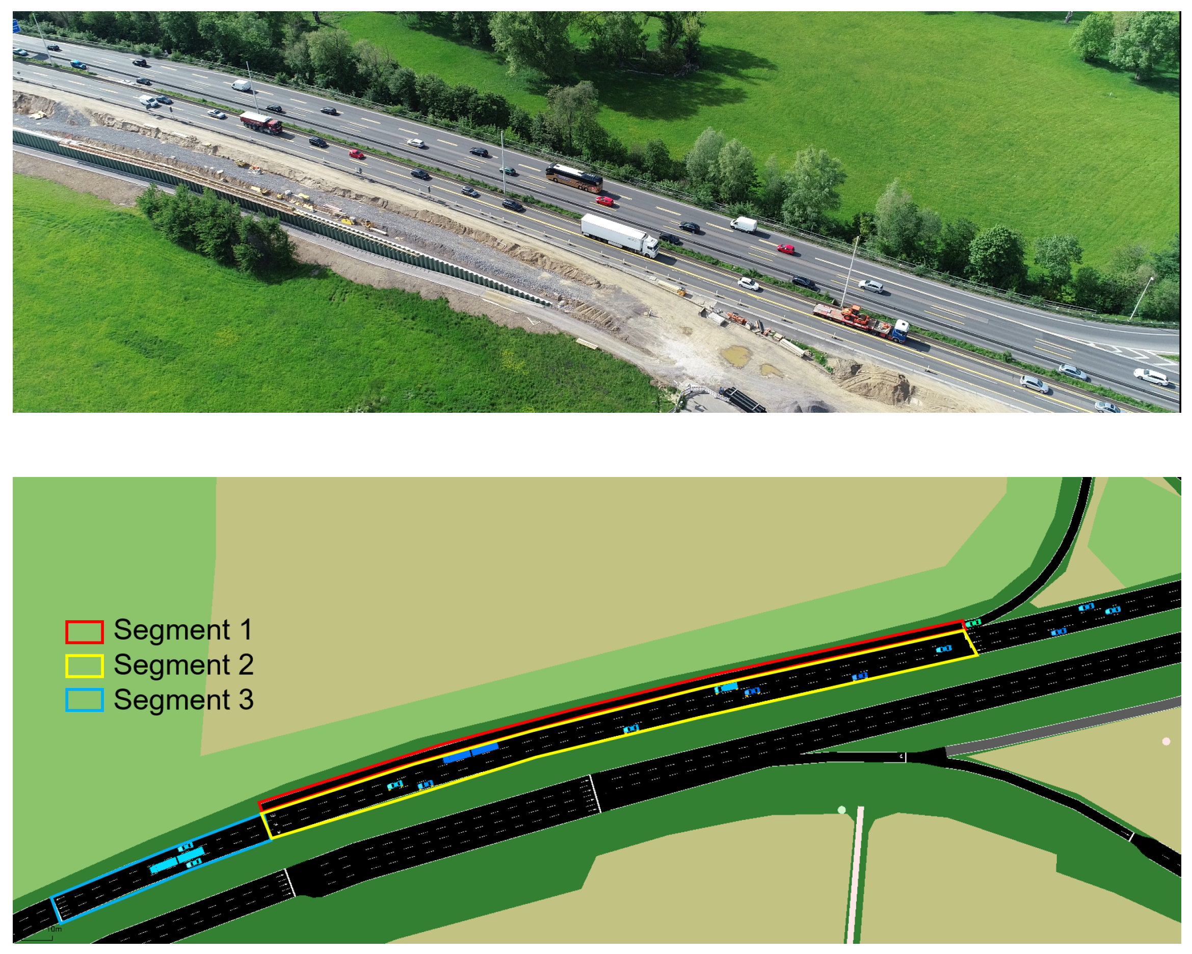
2.1. Trajectory Data

For the analysis, we used real vehicle trajectories recorded by drone photography from the German freeway A565 near the interchange Bonn-Beuel in May 2019; see Figure 2 (top) [34]. Vehicle types and trajectories were obtained using image processing, after which the raw data points were interpolated using third-order polynomials. A stretch of approximately 270 m covering (including the entry lane) 4 unidirectional lanes was recorded. A total of 31 datasets were obtained from recordings over 4 days that took place either in the morning or in the afternoon, each one covering the traffic over periods of approximately 5 min. The number of entering vehicles varied with the time of day; on average, 44 vehicles passed the junction per minute throughout the data collection period. The macroscopic model was trained using the datasets 1, 4, 10, 11, 16, 19, 20, and 30. For the calibration of the new model, we used datasets 1–3, whereas for the comparison study, we used datasets 4–7. The latter groups were recorded at similar hours of the day with similar heavy vehicle percentage; see also Table A1 (Appendix A).

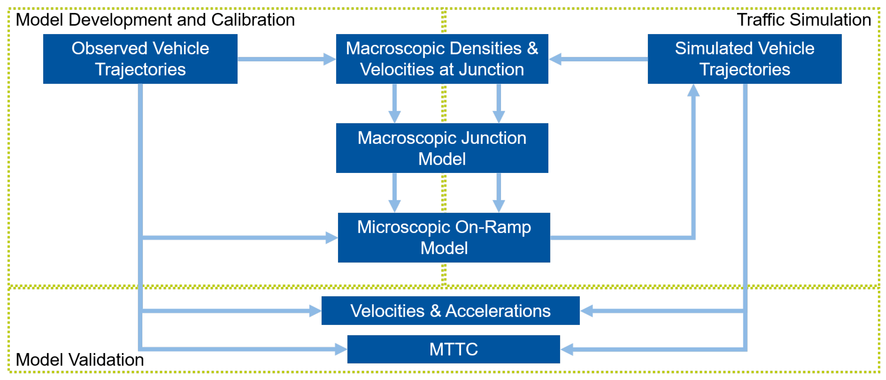
2.2. Data-Driven Macroscopic Junction Model

The macroscopic model we consider builds on the approach in [15]. Therein, a junction model has been introduced that relies on vehicle trajectory data. We describe the main idea of the model in this section, and we refer to [15] for a more detailed description. The model captures the scenario of an on-ramp on a motorway, which can be classified into the following three segments: (1) the entry lane allowing vehicles to enter the motorway, (2) the stretch of motorway before vehicles from the entry lane can enter, and (3) the stretch of motorway at which vehicles from the on-ramp enter or have entered the freeway. Segments 2 and 3 amount to a short stretch, at which no further on-ramps or exits are located, corresponding to the previously described dataset in which these segments have a total length of approximately 300 m. The segments are shown in Figure 2 (bottom).
In the macroscopic model description, no distinction between the individual lanes within the segments is made (the on-ramp consists of a single lane, while both segments 2 and 3 cover three lanes). At each segment, the traffic is governed by the Lighthill–Whitham–Richards (LWR) model
ρ t + ( ρ v s ( ρ ) ) x = 0 ,
which describes the time and space dependent traffic density by means of a partial differential equation [5]. In our application, only a single space variable was considered. From the trajectory data, vehicle numbers were counted in fixed control volumes, and their average velocities were computed, which allowed us to fit the parameters v max s and ρ max s of the Greenshields fundamental diagram
v s ( ρ ) = v max s 1 ρ ρ max s
for each of the three segments, i.e., for s = 1 , 2 , 3 . As both the LWR model and the Greenshields fundamental diagram have been found to be limited in fitting time-and-space-dependent vehicle densities on motorways, we emphasize that in our overall framework, they were not used to predict the tempo-spatial behavior of all vehicles but to derive further information on the interaction between vehicles on different segments of the on-ramp. The model assumes that the three segments meet, and therefore, the traffic densities couple at a single fixed spatial point. The coupling is modeled by means of a Riemann solver
R S : ( ρ 0 1 , ρ 0 2 , ρ 0 3 ) ( Q 0 1 , Q 0 2 , Q 0 3 )
that maps densities adjacent to the junction to coupling fluxes that govern the behavior at the junction. In numerical simulations, the Riemann solver is applied to trace data at a given time t in order to compute boundary fluxes at the time t + Δ t . A plethora of such coupling models has been evaluated; for simplicity, we focus in this work on the flow maximization approach [35], which maximizes the flux at the junction while assuring that both Kirchhoff conditions, as well as the demand and supply conditions [36], which depend on the fundamental diagrams corresponding to the three segments, hold. These conditions ensure mass conservation at the junction. The coupling model includes additional parameters that have been estimated using the traffic data and numerical simulations. The latter has been conducted using an adapted Lax–Friedrichs scheme. As the model has been originally calibrated to the same on-ramp data that are considered in this work, it was used here with all estimated parameters as the basis for a novel microscopic ramp model.

2.3. Transformation to Microscopic Model

We consider a car-following model that determines the vehicle accelerations, which we denote as a, based on the longitudinal positions (x), velocities (v), and vehicle lengths (L) of a vehicle pair (leader with index L and follower with index F on the same lane), i.e.,
a F = f ( x L , x F , v L , v F , L L , L F ) ,
where the function f is specified below. A car-following model combines Equation (4) with the kinematic relationships a F = v F ˙ and v F = x F ˙ , giving rise to a system of ordinary differential equations (ODEs) [37]. After discretizing these relations in time, the model is stated using the ballistic update formulas for speed and position of a follower; see, e.g., [38]:
v F ( t + Δ t ) = v F ( t ) + a F ( t ) Δ t ,
x F ( t + Δ t ) = x F ( t ) + Δ t 2 ( v F ( t ) + v F ( t + Δ t ) ) .
In the following, we include information from the macroscopic model in the car-following model (5). Therefore, we note the following relations: the flow is the inverse of the mean (gross) time headway ( Q = 1 / T ) at a specific location, i.e., the difference between the times when two subsequent vehicles reach a fixed reference point. The density is the inverse of the mean (gross) spacing ( ρ = 1 / S ) at a specific time, and the spacing S here refers to the difference between the positions of two subsequent vehicles. The macroscopic fundamental equation of traffic flow ( Q = v ρ ) thus takes the following form:
v = S T .
Equation (7) holds for the mean speed, spacing, and time headway, as well as for the speed, spacing, and time headway of individual vehicles. We use the equation to model the speed of microscopic vehicles within a predefined stretch of road at the time t + Δ t from the spacing and the flow at time t, as predicted by the macroscopic model:
v ˜ F ( t ) = S ( t ) Q ( t ) = x L ( t ) x F ( t ) L L + L F 2 Q ( t ) .
Here, L L and L F denote the lengths of the leading and the following vehicles, respectively. The flow is obtained using (3). As a macroscopic quantity, the flow is the same for all vehicles at the considered stretch of road, but the spacing may be different depending on the traffic conditions at time t. Taking into account Equation (7), the speed of the vehicles on the stretch may differ. The flow Q ( t ) in (8) is obtained from the macroscopic coupling model (3) using densities computed from the current vehicle positions on the on-ramp as input.
To avoid sudden speed changes, we model the acceleration using the Full Velocity Difference Model (FVDM) by [17] using the formula
a F ( t ) = v ˜ F ( t ) v F ( t ) τ λ ( v F ( t ) v L ( t ) ) .
The first term accounts for vehicle acceleration proportional to the difference between its current speed and the target speed. The second term introduces a reduction proportional to the speed difference between leader and follower to avoid collisions if the leader is very slow. In Equation (9), the adaptation time that determines the sensitivity to speed differences between the current and the modeled speed is denoted by τ , and the sensitivity to speed differences between leader and follower is denoted by λ . Note that we only adopt the principle of the FVDM, but we employ the speed v ˜ F from the macroscopic model. Unlike the macroscopic model, the microscopic car-following model allows for different accelerations for each vehicle.
For segments 2 and 3 (see Figure 2 bottom), where vehicles mainly follow the leader on the same lane, this model can be directly applied. For the on-ramp (segment 1), however, there are two additional phenomena that require modifications: (1) vehicles on the entry lane adapt their speed and spacing to the vehicles on the adjacent through lane, and (2) vehicles on the through lane may reduce their speed and increase the gap when a vehicle on the on-ramp wants to merge. These effects are not considered in the macroscopic model, and they are therefore not included in the microscopic model presented so far. We model these two phenomena microscopically by virtually combining the entry lane and the adjacent through lane to a single lane. This means the leader is the closest vehicle in front on either lane, and the flow is the sum of the flows on these two lanes. At the end of the entry lane, the assumption that both lanes can be combined is justified, because vehicles on the entry lane merge to the through lane and therefore need to adapt their behavior to the vehicles on the through lane. At the start of the entry lane, however, vehicles are still allowed to overtake and to maintain small gaps with respect to vehicles on the adjacent lane. We model this behavior using an adaptation time that decreases as the vehicles are passing the on-ramp using the formula
τ = x E x F v F
with x E denoting the position of the end of the entry lane.

2.4. Model Implementation

We used SUMO to simulate the previously recorded traffic on an on-ramp in Germany (see Figure 2). SUMO is an extendable open-source traffic simulation software [39]. The road network was modeled using input data from OpenStreetMap. As a result, the simulated road has the same course, and the entry lane has the same length as in the real traffic scenario. The width of the lanes was consistently 3.0 m, and only the leftmost lane was 2.6 m wide. The microscopic model was implemented using SUMO’s traffic control interface (TraCI). For the evaluation of the proposed flow-based model’s performance, we also simulated traffic using the IDM [18] as the car-following model combined with Erdmann’s model [40], which is the default lane change model in SUMO. For both the IDM and Erdmann’s lane change model, we used the default model parameters of SUMO. The traffic demand was taken from a 15 min excerpt of the vehicle trajectory dataset of the real road section [34]. For both the microscopic flow-based model and IDM, we used four vehicle types: Passenger cars, vans, trucks, and buses. Our flow-based model employed vehicle positions and velocities that were extracted from SUMO at every time step (0.1 s). From the positions of the vehicles, the densities were computed as a moving average over 15 s. The densities are the input for (3), which yields the flows. The flows were then used to compute the speeds for all individual vehicles according to (8). The speeds predicted by the models were afterwards fed back into SUMO to adapt the speeds of the vehicles in segments 1 to 3. Outside of these segments (in front of and behind the on-ramp), vehicles behaved according to the IDM.
Although we modeled the driving behavior at on-ramps, our model does not explicitly contain lane changes. Instead, the car-following model implicitly ensures that lane changes are possible by letting the vehicles on the entry lane adapt to the vehicles on the right through lane and vice versa. The lane changes are triggered by SUMO’s default lane change model [40], which ensures that lane changes are only conducted when there is a sufficient gap on the target lane. In the case of mandatory (also called strategic) lane changes, the model takes into account the speed, the remaining distance to the end of the lane, and the density on the current and target lane to determine when the lane change is executed. If the time until the merging vehicles reach the end of the on-ramp is smaller than the lane change duration (4 s), then the merging vehicles are forced to start a lane change using TraCI. This approach was used for both our model and the IDM, which allowed us to only evaluate the car-following properties of the two models.
Microscopic traffic flow models can be calibrated on both the microscopic and the macroscopic scale. While microscopic calibration is potentially more accurate, macroscopic calibration is more robust and does not require detailed trajectory data. Therefore, we used macroscopic calibration in this study. The model parameters of the macroscopic model have been calibrated in a previous study [15]. The value of parameter λ in the FVDM was adopted from the literature [41] ( λ = 0.3 ). For the comparison scenario with the IDM, the default parameter values in SUMO were used.

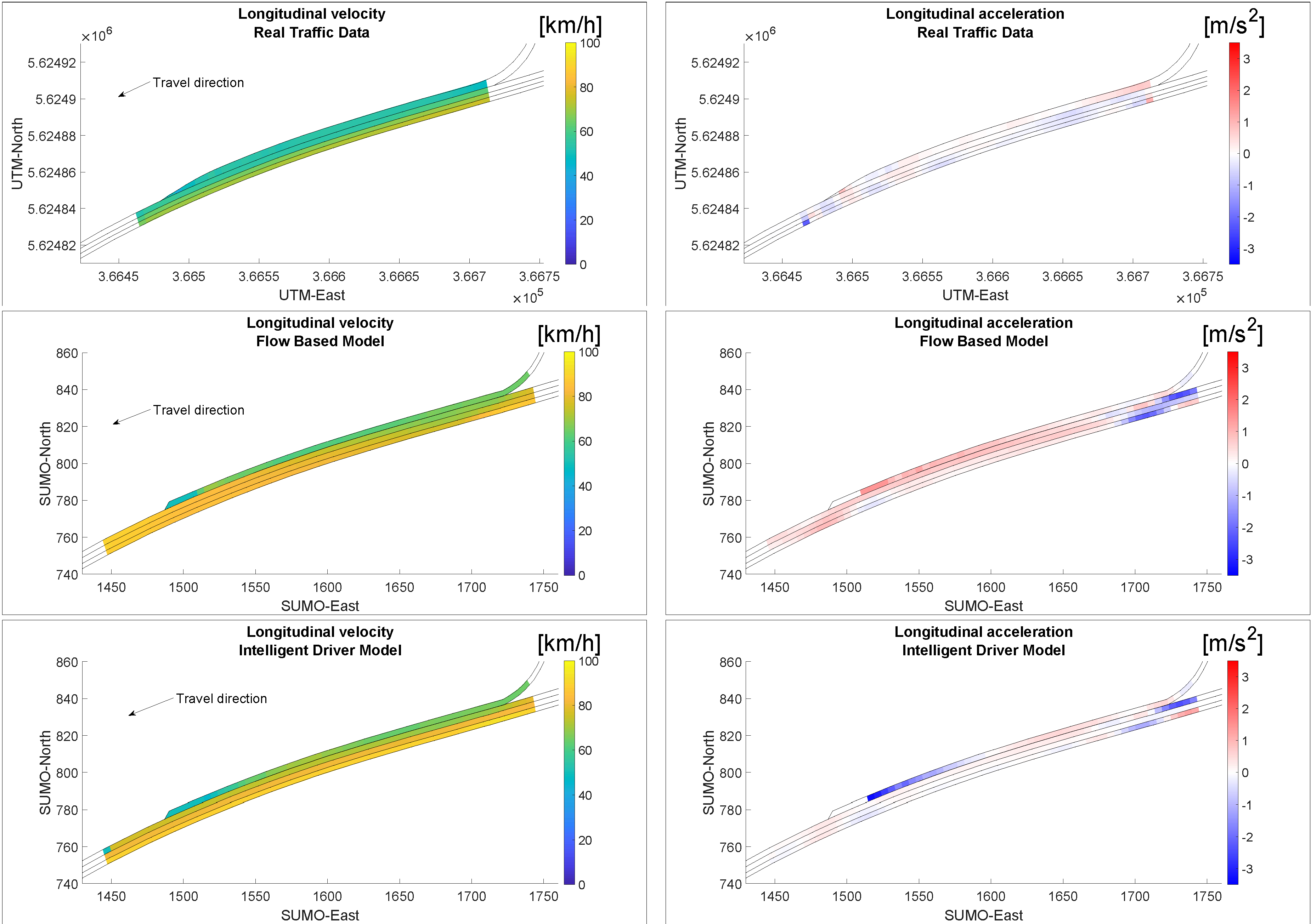
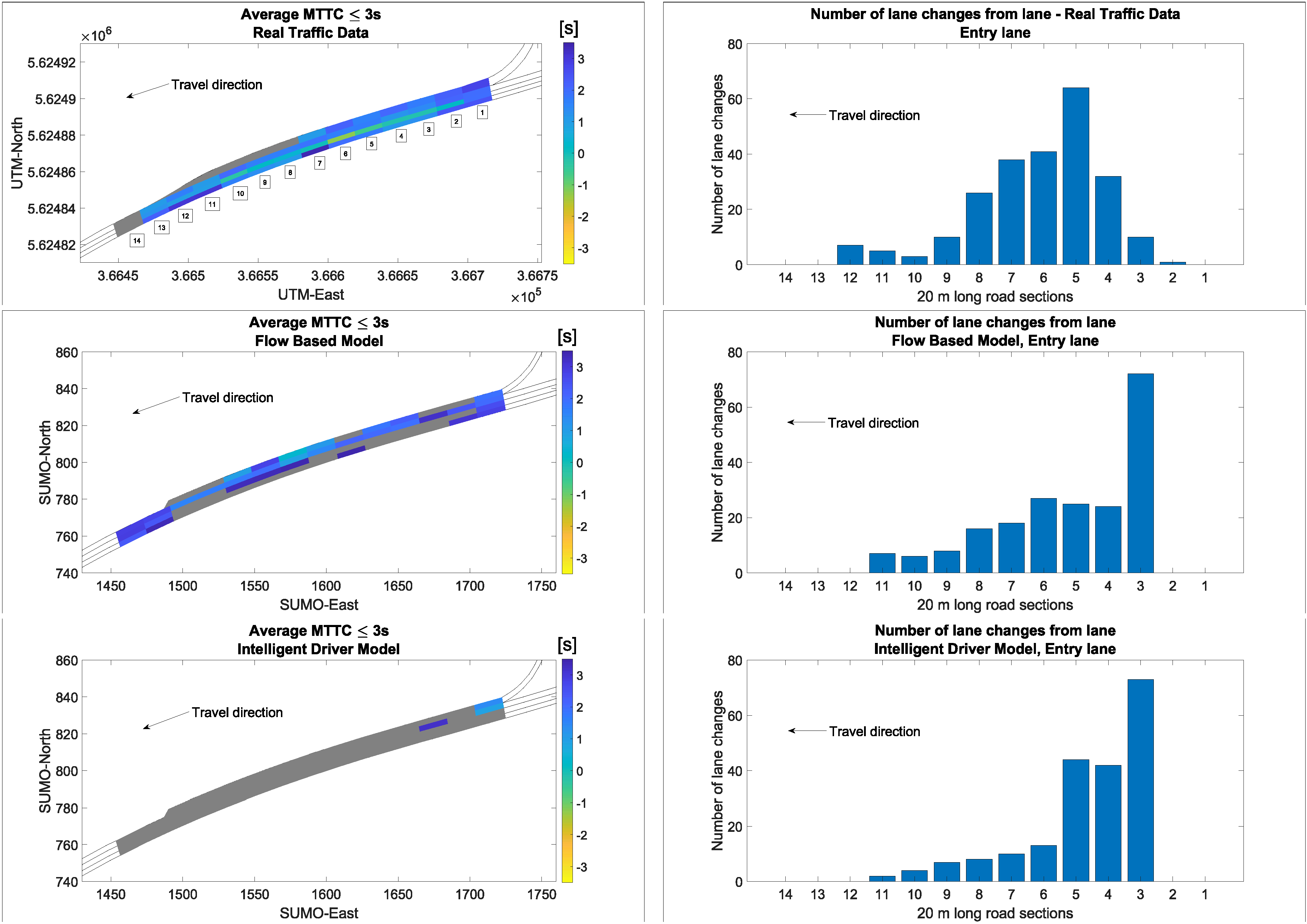
2.5. Model Evaluation

For the model evaluation, we prepared the simulated traffic data in the same structure as the real traffic data. The simulation results contain information about each vehicles’ category, size, location, speed, and acceleration, with the latter three being recorded every 0.2 s. The location information is given in SUMO’s global coordinate system.
When vehicles on the main lane approach the on-ramp, they might adjust their behavior for a smoother flow, extending the available gap to help vehicles to merge onto the motorway. Therefore, we looked at the speed and acceleration profiles, the lane changes, and the risky interactions in the different scenarios to validate the performance of the microscopic model in reproducing the real traffic data and in comparison to the IDM. The location of the lane changes and the changes in speed and acceleration along road sections can indicate how well a traffic model simulates traffic on the microscopic level. For an insight, we created 5 m long sections on each lane to calculate the average local speed and average local acceleration values. Similarly, we created 20 m long sections where we counted the number of lane changes.
On motorways, vehicles are mostly involved in rear-end conflict. In those cases, the application of surrogate safety measures to evaluate an interaction seems straightforward: There is a leader and a follower vehicle involved travelling behind each other in this explicit order. However, while changing lanes, often it is ambiguous which vehicle will take the ‘leading’ role. The determination of vehicle order or even the prediction of involvement of vehicles on the target lane becomes even more difficult when acceleration behavior is considered. Usually, vehicles accelerate on entry lanes and decelerate on main lanes for smoother merge. To overcome the complexity of vehicle pair prediction in lane-changing situations, we defined vehicle pairs from the moment the position of the changing vehicle’s left or right corner (assuming a rectangularly shaped vehicle) crossed the lane marking, even though its center point was still on the original lane. This predicts the gap in which the changing vehicle is most likely going to merge.
We used modified Time-to-Collision to evaluate vehicle interactions from the safety point of view. Time-to-Collision (TTC) is one of the most widely used surrogate safety measure, which calculates the nearness to a collision in seconds based on the actual speed and initial net distance of following vehicles, supposing that none of the vehicles would change their course [42]. The modified version of TTC, MTTC, was developed in [43] and additionally takes into account the initial acceleration behavior of both interacting vehicles, leading to a more realistic estimation. MTTC is defined as the smallest real and positive t such that
1 2 a L t 2 + v L t + x L = 1 2 a F t 2 + v F t + x F L L + L F 2
holds or as infinity if no such t exists.
We calculated MTTC between vehicle pairs in car-following and lane-changing situations as described above every 0.2 s. After determining the gap a lane-changing vehicle would merge into, we calculated the collision point based on the current collision angle [44]. To see the development of risky interactions along the road, we calculated the average MTTC under 3 s with respect to the predefined 20 m long sections. Therefore, we assigned a leader–follower pair to the road section corresponding to the current position of the follower and took the minimal MTTC of that pair during the time the follower drove in that section. Then, for each road segment, the average over these values if under or equal to 3 s was computed.

3. Results and Discussion

To evaluate the proposed model, we compared real traffic data on the on-ramp (see Trajectory data) to simulations conducted with the new flow-based model, as well as simulations conducted with the IDM; see Model Implementation. Our analyses focused on the spatial variations of traffic dynamics and therefore considered temporal averages of key quantities with respect to the position on the on-ramp setting. To achieve this, we divided the road longitudinally into 5 m long sections.
First, we analyzed the (longitudinal) velocities along the on-ramp. Figure 3 (left) shows that due to limited accuracy of the calibration, both models overestimated the velocities of real traffic. The models, however, accurately represented the fact that the velocities on the on-ramp lane are smaller than on the through lanes. Comparing both models, we found that the variance in velocity between the lanes, which in the data ranged from 52.65 km/h on the entry lane to 72.02 km/h on the second passing lane, was better represented by the new model predicting a range from 64.28 km/h to 82.66 km/h. Unlike the IDM, it assumed that the largest difference in average velocity was between the on-ramp and the main lane (from 64.28 km/h to 77.54 km/h), while in the data, only a minor difference (52.65 km/h to 56.40 km/h) was observed. The largest difference in average velocities in the data was observed between the main lane and the first passing lane (from 56.40 km/h to 67.05 km/h), which was also the case in the simulations by the IDM, predicting a jump from 73.25 km/h to 81.36 km/h. These different model results might occur because the new model does not explicitly include differences between the through lanes. In reality, these speed differences occur not only due to the on-ramp, but they also occur due to different desired speeds of the individual vehicles. This heterogeneity was not considered in our simulations.
In terms of acceleration, Figure 3 (right) shows that both models predicted larger absolute accelerations compared to the data. This means that the observed behavior that drivers adapt their speed to the forthcoming on-ramp and therefore avoid large accelerations was not reflected in both models. In other words, both models tend to predict aggression regarding acceleration and reactive, i.e., less anticipatory, driver behavior. Since our model is derived from a macroscopic model, not explicitly accounting for acceleration, additional model assumptions in the future might achieve more realistic accelerations. Furthermore, we note that our model was only calibrated on the macroscopic scale and that the IDM was used with SUMO’s default values. Detailed microscopic calibration, which has not been realized in this analysis due to its large computational cost and complexity, could be helpful to find a suitable balance between the two acceleration terms in Equation (9) and therefore obtain more realistic accelerations.
Figure 3 (right) also shows that in the results of our model, the vehicles on the through lanes decelerated significantly in front of the on-ramp section to allow vehicles from the right to merge. This phenomenon can also be observed in real traffic data, but to a smaller extent. Moreover, the IDM produced large negative accelerations at the end of the on-ramp lane, because vehicles stop and wait for a suitable gap if they have not found one before. Our proposed model does not show this unrealistic behavior.
In the real traffic data and the traffic simulated with the considered models, no accident occurred, which calls for further measures to evaluate the traffic safety evaluation. With the help of Surrogate Safety Measures, areas with higher collision risk can be identified. Figure 4 (left) shows the average MTTC values under 3 s within a given 20 m long section (see the Model Evaluation section for details). If the average within these sections lies above 3 s, it indicates a safe, conflict-free area. In this case, the section is colored gray.
The real traffic data exhibited the lowest MTTCs and therefore the riskiest traffic scene. In the traffic simulated with the new model, the entry and main lane displayed the most dangerous area, but there was little to no disturbance on the two passing lanes. In the traffic simulated with the IDM, only the first 20 m long sections on both the on-ramp and the main lane showed low average MTTCs, while the rest of the analyzed stretch remained safe.
Figure 5 (left) shows the average MTTCs of the lanes: We computed the average over 20 m long sections on the considered on-ramp scenario combining all lanes. Comparing the two models, we see that only three out of 15 sections have average MTTCs that are less than 3 s in the case of the IDM model, and thus, generally safe driving behavior is assumed. The new flow-based model predicted results that are more similar to the observed traffic scene in the data locally involving riskier driving behavior. Compared to real traffic, the new model exhibited multiple locations at which a lower MTTC was pronounced. Figure 5 (right) shows the total number of sections that had an average MTTC between 0–1.5 s, 1.5–2 s, 2–2.5 s, 2.5–3 s, and above 3 s. While the distribution of average MTTC achieved by the flow-based model differs from the one of the real traffic data, this is mainly because of the small number of conflicts on the passing lanes that the model predicted. Figure 4 (right) visualizes the changes from the entry lane to the main lane with respect to their location in the 20 m long sections on the considered on-ramp. In the simulations of the IDM model, vehicles preferably change to the main lane as soon as possible. While a large part of the vehicles also changed very early in the simulation results of the flow-based model, more changes occurred toward the end of the on-ramp, which is closer to the observed behavior in the data.
To investigate how the macroscopic calibration would affect the microscopic model, we conducted simulations varying the maximum density of segment 2, with ρ m a x 2 . Figure 6 shows that the deviation between the real traffic data and simulated traffic with respect to the mean velocity and density on the main lane was smallest when the calibrated value of ρ m a x 2 was used. A larger ρ m a x 2 had only a minor impact on the deviation, while a smaller ρ m a x 2 led to a significant increase in the deviation, as congestion was predicted in the first half of the considered time span. This indicates that our macroscopic calibration has been suitable to obtain a valid microscopic model.

4. Conclusions

In this paper, we proposed a microscopic car-following model for on-ramps derived from a macroscopic traffic flow model. The macroscopic model was calibrated based on real traffic data collected at a highway junction in Germany. The microscopic model includes a few additional assumptions for the acceleration and synchronization between the on-ramp and the adjacent lane, which are neglected in macroscopic models, in order to ensure realistic merging behavior at on-ramps. To the best of our knowledge, our model is the first approach to include possibly risky merging behavior from traffic data in a microscopic simulator. By evaluating the proposed model in a traffic simulation, we found that the speeds and accelerations were larger than in real traffic, but they were more realistic than in the Intelligent Driver Model. The distribution of the lane change positions was also more realistic than in the IDM. The proposed model is suitable for road safety analysis, as it creates a realistic amount and severity of conflicts. For example, it can be applied to evaluate different designs of on-ramps (regarding lengths, speed limits, ramp-metering strategies, etc.) in traffic simulations by incorporating fitted on-ramp models of comparable on-ramp situations in microscopic simulations. On a larger scale, the composition of various microscopic merging models of this kind into complex motorway junctions might assist in evaluating the throughput for different architectures. Since the calibration was only performed on the macroscopic level, the accelerations in both the IDM and the flow-based model were larger than in the real data. With microscopic calibration, which involves an expensive fitting of the parameters λ and τ , a better resemblance between the model and the real traffic might be achieved in future work. As it stands, extensive vehicle trajectory data at on-ramps have been scarce to come by, and the recording and image processing of the considered data have been costly (see Section 2.1). Further validation will be necessary in future work. We note, however, that given suitable data, the presented framework is transferable to similar on-ramps and junctions, at which two road segments merge into a third one, as shown in Figure 2. Extended geometries and different types of junctions require model extensions on the macroscopic scale, as well as more data for their calibration. The current study serves as a proof of concept, as only the flow maximization junction model has been considered; further modeling approaches including data driven neural networks could be considered.
Combining the advantages of both macroscopic and microscopic models is a promising approach to obtain models that represent both microscopic driver behavior and macroscopic traffic phenomena well. However, even with thorough calibration, on-ramps remain a challenging road section to model.

Author Contributions

Conceptualization, N.K., M.B. and E.K.; Formal analysis, N.K., M.B. and E.K.; Funding acquisition, M.H. and M.O.; Investigation, N.K., M.B. and E.K.; Methodology, N.K., M.B. and E.K.; Supervision, M.H. and M.O.; Validation, N.K., M.B. and E.K.; Visualization, N.K., M.B. and E.K.; Writing—original draft, N.K., M.B. and E.K.; Writing—review and editing, M.H. and M.O. All authors have read and agreed to the published version of the manuscript.

Funding

The work presented in this paper is part of the project NeMo (Neue Ansätze der Verkehrsmodellierung unter Berücksichtigung komplexer Geometrien und Daten - New traffic models considering complex geometries and data), project number 461365406, funded by the German Research Foundation (DFG). NK and MH further thank the DFG for the financial support through 320021702/GRK2326, 333849990/IRTG-2379, B04, B05 and B06 of 442047500/SFB1481, HE5386/18-1,19-2,22-1,23-1,25-1, ERS SFDdM035, and under Germany’s Excellence Strategy EXC-2023 Internet of Production 390621612, as well as under the Excellence Strategy of the Federal Government and the Länder.

Data Availability Statement

The vehicle trajectory data used in this work have been published in [34].

Conflicts of Interest

The authors declare no conflicts of interest. The funders had no role in the design of the study; in the collection, analyses, or interpretation of data; in the writing of the manuscript; or in the decision to publish the results.

Appendix A

Table A1. Statistics on the on-ramp traffic for all datasets. Data were recorded in 2019 on May 13 (day 1), May 14 (day 2), May 15 (day 3), and June 21 (day 4). Modified from [15].
SetTimePeriodPassing VehiclesEntering Vehicles
nav. Speednav. Speed
1day 15:10:305 min, 25 s28174.9 km/h5266.1 km/h
2day 15:15:575 min, 26 s30174.3 km/h7163.5 km/h
3day 15:21:245 min, 32 s29871.0 km/h7162.3 km/h
4day 15:43:575 min, 26 s31267.3 km/h7356.3 km/h
5day 15:49:255 min, 26 s28865.0 km/h7653.3 km/h
6day 15:54:525 min, 27 s28667.3 km/h6856.2 km/h
7day 16:00:221 min, 38 s2868.2 km/h349.4 km/h
8day 16:04:345 min, 26 s28267.7 km/h8956.3 km/h
9day 16:38:585 min, 26 s26967.4 km/h6456.9 km/h
10day 16:44:261 min, 25 s6348.8 km/h1132.2 km/h
11day 215:10:372 min, 45 s8574.4 km/h1861.7 km/h
12day 215:26:355 min, 27 s21539.2 km/h3333.3 km/h
13day 215:44:395 min, 27 s23366.3 km/h5054.7 km/h
14day 215:50:075 min, 27 s23573.0 km/h5461.0 km/h
15day 215:55:342 min, 22 s10773.3 km/h2963.8 km/h
16day 216:02:445 min, 27 s25073.5 km/h6962.6 km/h
17day 216:08:135 min, 26 s24474.2 km/h5961.4 km/h
18day 216:19:243 min, 6 s14967.3 km/h3761.4 km/h
19day 36:07:225 min, 27 s30065.2 km/h8954.4 km/h
20day 36:12:515 min, 26 s27863.8 km/h8352.2 km/h
21day 37:26:132 min, 39 s6667.4 km/h758.7 km/h
22day 415:28:145 min, 26 s22172.5 km/h2760.5 km/h
23day 415:33:425 min, 26 s24772.3 km/h2061.9 km/h
24day 415:39:095 min, 26 s23073.7 km/h1562.5 km/h
25day 415:44:362 min, 48 s7667.8 km/h458.9 km/h
26day 416:06:022 min, 59 s7968.6 km/h963.2 km/h
27day 416:11:535 min, 26 s23177.3 km/h3162.3 km/h
28day 416:33:195 min, 27 s23174.3 km/h2962.2 km/h
29day 416:38:475 min, 27 s24468.2 km/h3857.1 km/h
30day 416:44:155 min, 27 s24873.0 km/h3462.0 km/h
31day 416:49:454 min, 34 s17168.6 km/h1454.7 km/h

References

  1. Blazek, D.; Blazekova, O.; Vojtekova, M. Analytical model of road bottleneck queueing system. Transp. Lett. 2022, 14, 888–897. [Google Scholar] [CrossRef]
  2. Mahmud, S.S.; Ferreira, L.; Hoque, M.S.; Tavassoli, A. Micro-simulation modelling for traffic safety: A review and potential application to heterogeneous traffic environment. IATSS Res. 2019, 43, 27–36. [Google Scholar] [CrossRef]
  3. Storani, F.; Di Pace, R.; de Luca, S. A hybrid traffic flow model for traffic management with human-driven and connected vehicles. Transp. B Transp. Dyn. 2022, 10, 1151–1183. [Google Scholar] [CrossRef]
  4. Aw, A.; Rascle, M. Resurrection of Second Order Models of Traffic Flow. SIAM J. Appl. Math. 2000, 60, 916–938. [Google Scholar] [CrossRef]
  5. Lighthill, M.J.; Whitham, G.B. On kinematic waves II. A theory of traffic flow on long crowded roads. Proc. R. Soc. Lond. Ser. A Math. Phys. Sci. 1955, 229, 317–345. [Google Scholar] [CrossRef]
  6. Richard, P.I. Shock Waves on the Highway. Oper. Res. 1956, 4, 42–51. [Google Scholar] [CrossRef]
  7. Zhang, H.M. A non-equilibrium traffic model devoid of gas-like behavior. Transp. Res. Part B Methodol. 2002, 36, 275–290. [Google Scholar] [CrossRef]
  8. Fan, S.; Herty, M.; Seibold, B. Comparative model accuracy of a data-fitted generalized Aw-Rascle-Zhang model. Netw. Heterog. Media 2014, 9, 239–268. [Google Scholar] [CrossRef]
  9. Schönhof, M.; Helbing, D. Empirical Features of Congested Traffic States and Their Implications for Traffic Modeling. Transp. Sci. 2007, 41, 135–166. [Google Scholar] [CrossRef]
  10. Würth, A.; Binois, M.; Goatin, P.; Göttlich, S. Data-driven uncertainty quantification in macroscopic traffic flow models. Adv. Comput. Math. 2022, 48, 916. [Google Scholar] [CrossRef]
  11. Garavello, M.; Piccoli, B. Traffic Flow on Networks: Conservation Law Models; American Institute of Mathematical Sciences: Pasadena, CA, USA, 2006. [Google Scholar]
  12. Göttlich, S.; Herty, M.; Moutari, S.; Weissen, J. Second-Order Traffic Flow Models on Networks. SIAM J. Appl. Math. 2021, 81, 258–281. [Google Scholar] [CrossRef]
  13. Simoni, M.D.; Claudel, C.G. A Fast Lax–Hopf Algorithm to Solve the Lighthill–Whitham–Richards Traffic Flow Model on Networks. Transp. Sci. 2020, 54, 1516–1534. [Google Scholar] [CrossRef]
  14. Herty, M.; Kolbe, N.; Müller, S. Central schemes for networked scalar conservation laws. Netw. Heterog. Media 2023, 18, 310–340. [Google Scholar] [CrossRef]
  15. Herty, M.; Kolbe, N. Data-driven models for traffic flow at junctions. Math. Methods Appl. Sci. 2024, 47, 8946–8968. [Google Scholar] [CrossRef]
  16. Bando, M.; Hasebe, K.; Nakayama, A.; Shibata, A.; Sugiyama, Y. Dynamical model of traffic congestion and numerical simulation. Phys. Rev. Stat. Phys. Plasmas Fluids Relat. Interdiscip. Top. 1995, 51, 1035–1042. [Google Scholar] [CrossRef]
  17. Jiang, R.; Wu, Q.; Zhu, Z. Full velocity difference model for a car-following theory. Phys. Rev. Stat. Nonlinear Soft Matter Phys. 2001, 64, 017101. [Google Scholar] [CrossRef]
  18. Treiber, M.; Hennecke, A.; Helbing, D. Congested traffic states in empirical observations and microscopic simulations. Phys. Rev. Stat. Phys. Plasmas Fluids Relat. Interdiscip. Top. 2000, 62, 1805–1824. [Google Scholar] [CrossRef]
  19. Bham, G. A simple lane change model for microscopic traffic flow simulation in weaving sections. Transp. Lett. 2011, 3, 231–251. [Google Scholar] [CrossRef]
  20. Kong, D.; List, G.F.; Guo, X.; Wu, D. Modeling vehicle car-following behavior in congested traffic conditions based on different vehicle combinations. Transp. Lett. 2018, 10, 280–293. [Google Scholar] [CrossRef]
  21. Wang, Y.; Li, Y.; Li, R.; Wu, S.; Li, L. Unraveling Spatial–Temporal Patterns and Heterogeneity of On-Ramp Vehicle Merging Behavior: Evidence from the exiD Dataset. Appl. Sci. 2024, 14, 2344. [Google Scholar] [CrossRef]
  22. Zhang, D.; Chen, X.; Wang, J.; Wang, Y.; Sun, J. A comprehensive comparison study of four classical car-following models based on the large-scale naturalistic driving experiment. Simul. Model. Pract. Theory 2021, 113, 102383. [Google Scholar] [CrossRef]
  23. Mohan, R.; Ramadurai, G. State-of-the art of macroscopic traffic flow modelling. Int. J. Adv. Eng. Sci. Appl. Math. 2013, 5, 158–176. [Google Scholar] [CrossRef]
  24. Papageorgiou, M. Some remarks on macroscopic traffic flow modelling. Transp. Res. Part A Policy Pract. 1998, 32, 323–329. [Google Scholar] [CrossRef]
  25. Saifuzzaman, M.; Zheng, Z. Incorporating human-factors in car-following models: A review of recent developments and research needs. Transp. Res. Part C Emerg. Technol. 2014, 48, 379–403. [Google Scholar] [CrossRef]
  26. Colombo, R.; Rossi, E. On the Micro-Macro limit in traffic flow. Rend. Semin. Mat. Univ. Padova 2014, 131, 217–235. [Google Scholar] [CrossRef]
  27. Herty, M.; Fazekas, A.; Visconti, G. A two-dimensional data-driven model for traffic flow on highways. Netw. Heterog. Media 2018, 13, 217–240. [Google Scholar] [CrossRef]
  28. Herty, M.; Moutari, S.; Visconti, G. Macroscopic Modeling of Multilane Motorways Using a Two-Dimensional Second-Order Model of Traffic Flow. SIAM J. Appl. Math. 2018, 78, 2252–2278. [Google Scholar] [CrossRef]
  29. Wang, K.; Qu, D.; Yang, Y.; Dai, S.; Wang, T. Risk-Quantification Method for Car-Following Behavior Considering Driving-Style Propensity. Appl. Sci. 2024, 14, 1746. [Google Scholar] [CrossRef]
  30. Calvert, S.C.; Schakel, W.J.; van Lint, J. A generic multi-scale framework for microscopic traffic simulation part II—Anticipation Reliance as compensation mechanism for potential task overload. Transp. Res. Part B Methodol. 2020, 140, 42–63. [Google Scholar] [CrossRef]
  31. Mahmud, S.S.; Ferreira, L.; Hoque, M.S.; Tavassoli, A. Application of proximal surrogate indicators for safety evaluation: A review of recent developments and research needs. IATSS Res. 2017, 41, 153–163. [Google Scholar] [CrossRef]
  32. Tang, S.; Lu, Y.; Liao, Y.; Cheng, K.; Zou, Y. A New Surrogate Safety Measure Considering Temporal–Spatial Proximity and Severity of Potential Collisions. Appl. Sci. 2024, 14, 2711. [Google Scholar] [CrossRef]
  33. Dong, T.; Zhou, J.; Zhuo, J.; Li, B.; Zhu, F. On the Local and String Stability Analysis of Traffic Collision Risk. Appl. Sci. 2024, 14, 942. [Google Scholar] [CrossRef]
  34. Lamberty, S.; Fazekas, A.; Kalló, E.; Oeser, M. DROVA Dataset. 2023. Available online: https://data.isac.rwth-aachen.de/ (accessed on 20 August 2024).
  35. Garavello, M.; Han, K.; Piccoli, B. Models for Vehicular Traffic on Networks; AIMS Series on Applied Mathematics; American Institute of Mathematical Sciences: Springfield, MO, USA, 2016; Volume 9. [Google Scholar]
  36. Lebacque, J.P. The Godunov scheme and what it means for first order traffic flow models. In Proceedings of the 13th International Symposium on Transportation and Traffic Theory, Lyon, France, 24–26 July 1996; pp. 647–677. [Google Scholar]
  37. Keane, R.; Gao, H.O. Fast Calibration of Car-Following Models to Trajectory Data Using the Adjoint Method. Transp. Sci. 2021, 55, 592–615. [Google Scholar] [CrossRef]
  38. Treiber, M.; Kanagaraj, V. Comparing numerical integration schemes for time-continuous car-following models. Phys. A Stat. Mech. Its Appl. 2015, 419, 183–195. [Google Scholar] [CrossRef]
  39. Lopez, P.A.; Wiessner, E.; Behrisch, M.; Bieker-Walz, L.; Erdmann, J.; Flotterod, Y.P.; Hilbrich, R.; Lucken, L.; Rummel, J.; Wagner, P. Microscopic Traffic Simulation using SUMO. In Proceedings of the IEEE 2018 21st International Conference on Intelligent Transportation Systems (ITSC), Maui, HI, USA, 4–7 November 2018; pp. 2575–2582. [Google Scholar] [CrossRef]
  40. Erdmann, J. SUMO’s Lane-changing model. Lect. Notes Control. Inf. Sci. 2014, 13, 105–123. [Google Scholar]
  41. Berghaus, M.; Kallo, E.; Oeser, M. Car-Following Model Calibration Based on Driving Simulator Data to Study Driver Characteristics and to Investigate Model Validity in Extreme Traffic Situations. Transp. Res. Rec. 2021, 2675, 1214–1232. [Google Scholar] [CrossRef]
  42. Hayward, J.C. Near-miss determination through use of a scale of danger. Highw. Res. Rec. 1972, 384, 24–34. [Google Scholar]
  43. Ozbay, K.; Yang, H.; Bartin, B.; Mudigonda, S. Derivation and Validation of New Simulation-Based Surrogate Safety Measure. Transp. Res. Rec. J. Transp. Res. Board 2008, 2083, 105–113. [Google Scholar] [CrossRef]
  44. Nadimi, N.; Ragland, D.R.; Mohammadian Amiri, A. An evaluation of time-to-collision as a surrogate safety measure and a proposal of a new method for its application in safety analysis. Transp. Lett. 2020, 12, 491–500. [Google Scholar] [CrossRef]
Figure 1. Flow chart connecting the modeling, validation, and simulation techniques used in this work.
Applsci 14 09111 g001
Figure 2. Snapshot of the freeway A565 from a drone photograph (top) and our SUMO model (bottom). The on-ramp is situated on the topmost lane with travel direction from right to left. The segmentation of the on-ramp is indicated.
Applsci 14 09111 g002
Figure 3. Average longitudinal velocities (left) and accelerations (right) for real traffic data (top); the new flow-based model (center) and IDM (bottom).
Applsci 14 09111 g003
Figure 4. Left: average MTTC capped at 3s for real traffic data (top), the new flow-based model (center), and IDM (bottom). Sections with larger MTTC are colored gray. Right: distribution of longitudinal lane change positions from the entry lane to the main lane for real traffic data (top), the new flow-based model (center), and IDM (bottom).
Applsci 14 09111 g004
Figure 5. Left: average MTTC across all lanes with respect to their longitudinal section capped at 3 s for real traffic data (top), the new flow-based model (center), and IDM (bottom). Right: histogram of longitudinal sections with respect to their MTTC for real traffic data (top), the new flow-based model (center), and IDM (bottom).
Applsci 14 09111 g005
Figure 6. (left) Mean velocity on the main lane in simulations with varied ρ m a x 2 and in the traffic data. (right) Corresponding densities on the main lane.
Applsci 14 09111 g006
Disclaimer/Publisher’s Note: The statements, opinions and data contained in all publications are solely those of the individual author(s) and contributor(s) and not of MDPI and/or the editor(s). MDPI and/or the editor(s) disclaim responsibility for any injury to people or property resulting from any ideas, methods, instructions or products referred to in the content.

