
A 3D Two-Phase Landslide Dynamical Model on GIS Platform


Abstract
:1. Introduction
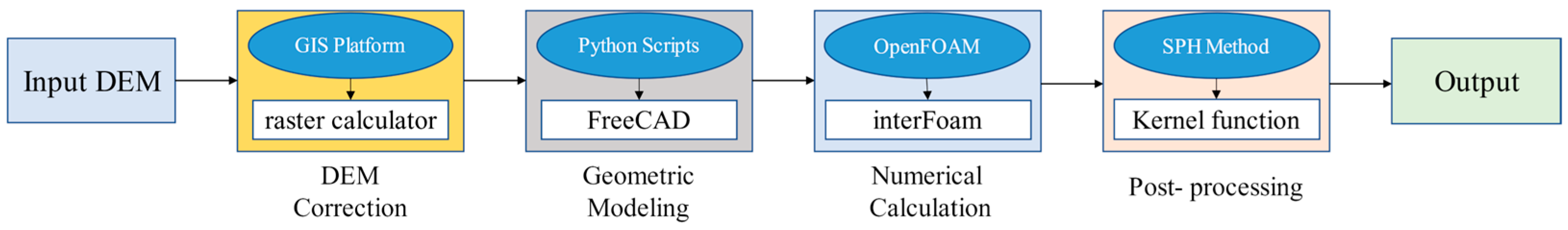
2. Methods
2.1. DEM Correction
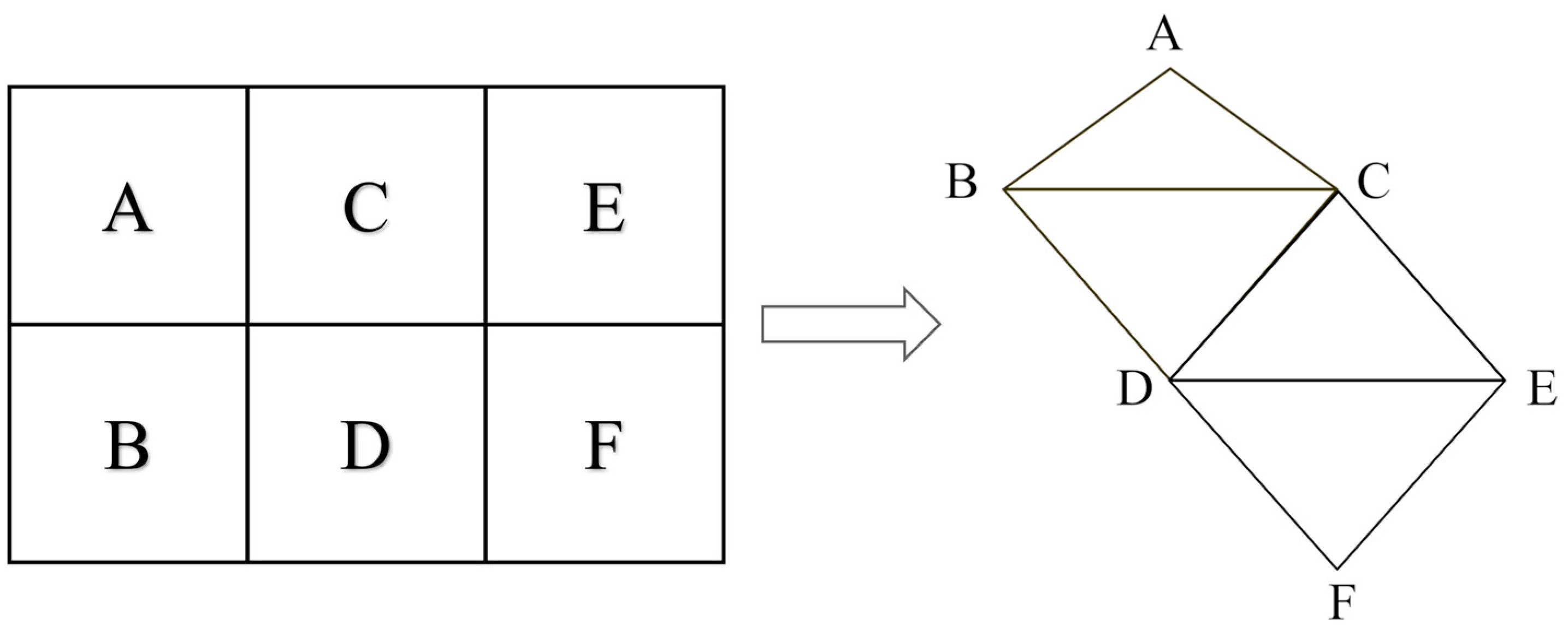
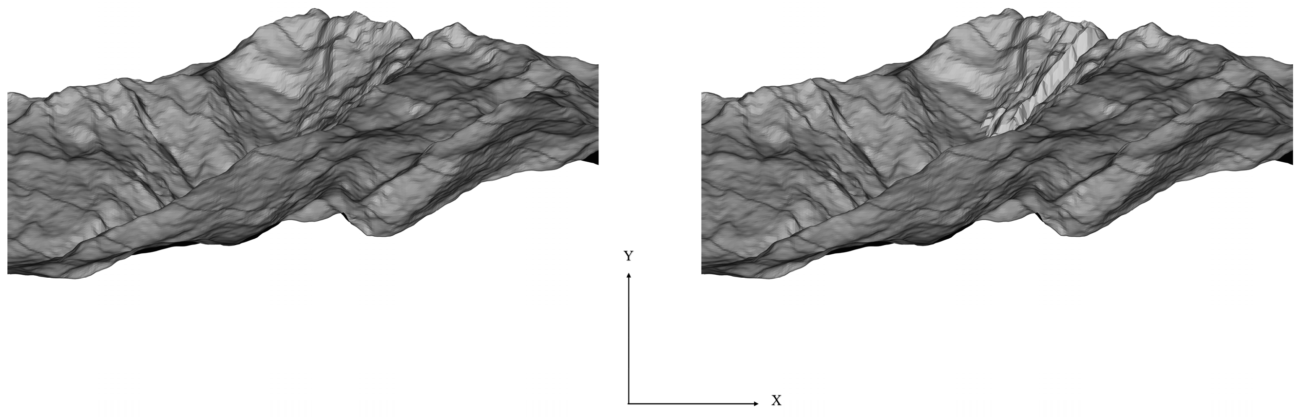
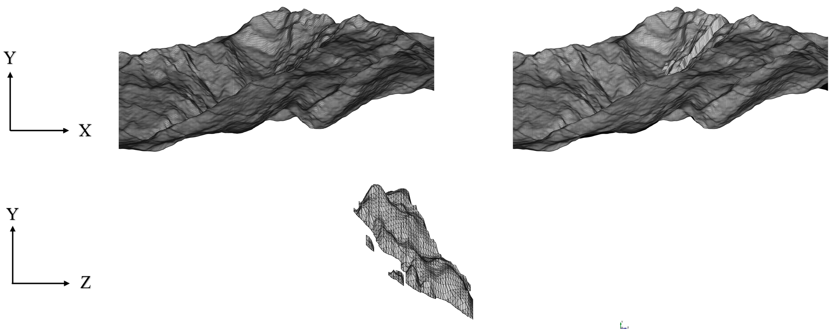
2.2. Geometric Modeling
2.3. Numerical Calculation
2.4. Post-Processing
3. Experimental Verification
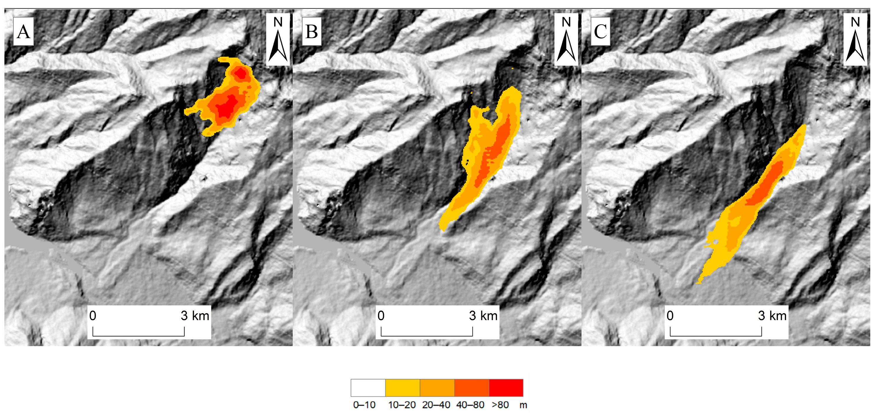
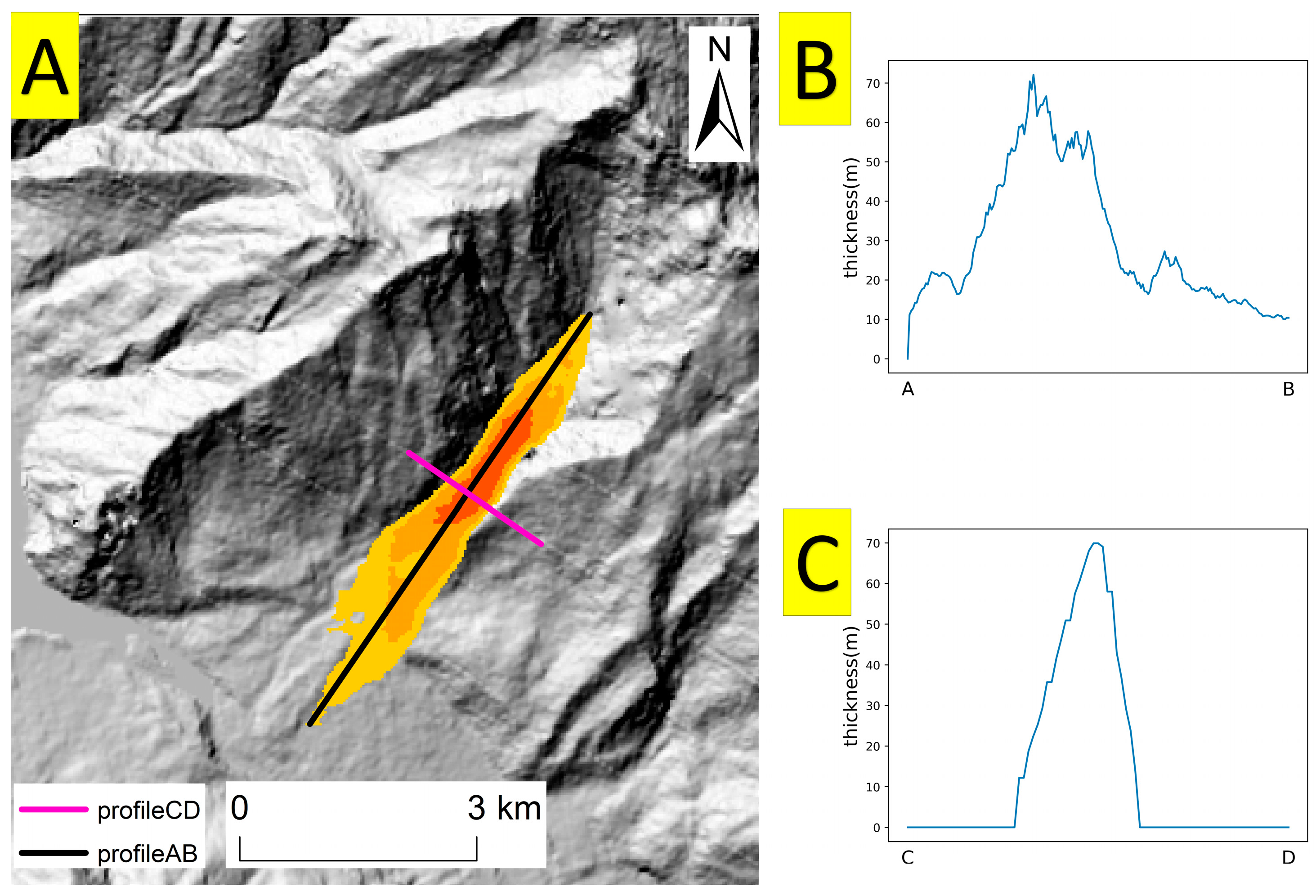
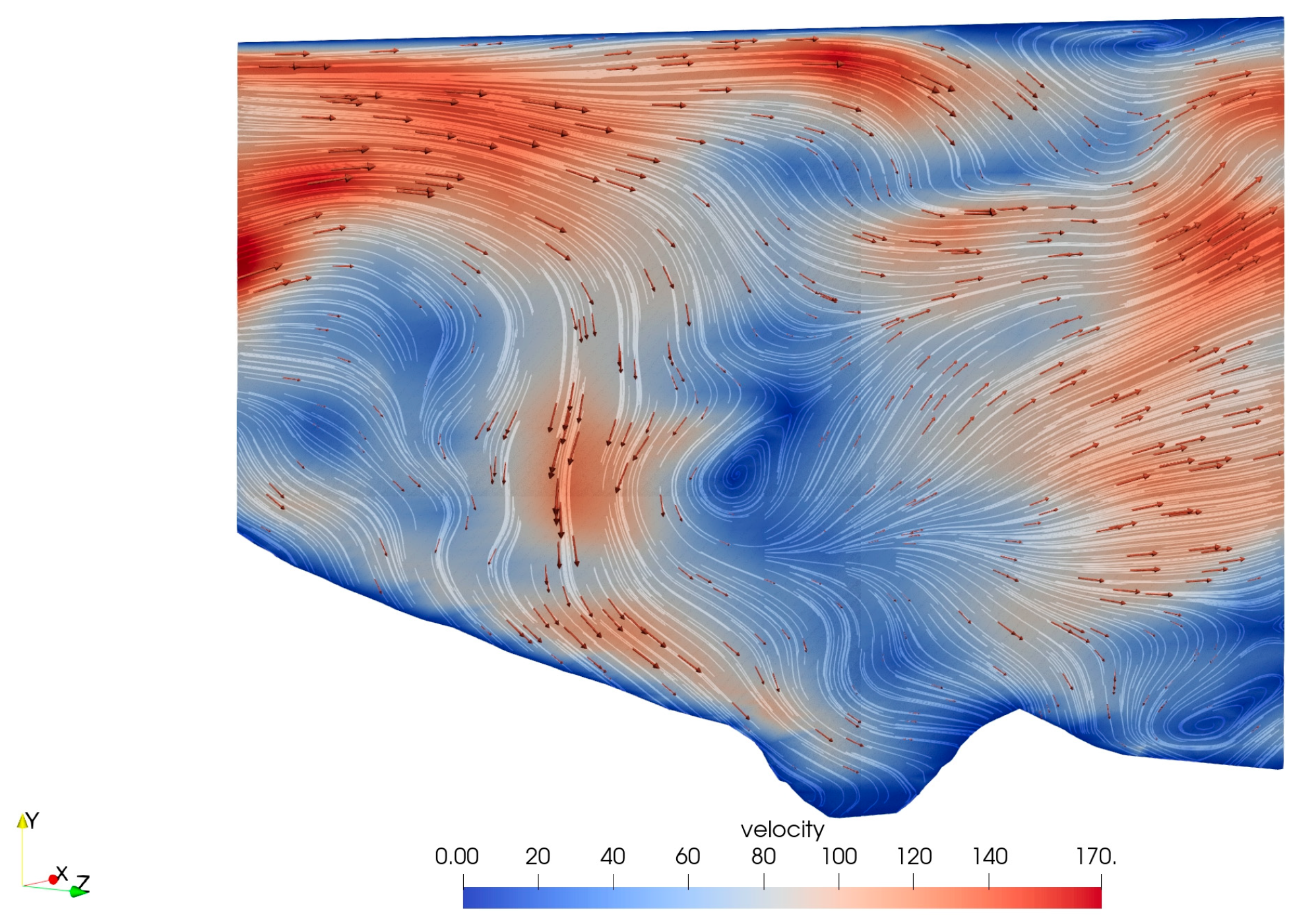
4. Results
5. Discussion
6. Conclusions
Author Contributions
Funding
Institutional Review Board Statement
Informed Consent Statement
Data Availability Statement
Conflicts of Interest
References
- Ouyang, C.J.; An, H.C.; Zhou, S.; Wang, Z.W.; Su, P.C.; Wang, D.P.; Cheng, D.X.; She, J.X. Insights from the failure and dynamic characteristics of two sequential landslides at Baige village along the Jinsha River, China. Landslides 2019, 16, 1397–1414. [Google Scholar] [CrossRef]
- Zhang, Y.; Chen, N.S.; Liu, M.; Wang, T.; Deng, M.F.; Wu, K.L.; Khanal, B.R. Debris flows originating from colluvium deposits in hollow regions during a heavy storm process in Taining, southeastern China. Landslides 2020, 17, 335–347. [Google Scholar] [CrossRef]
- Zhang, Z.; He, S.M.; Liu, W.; Liang, H.; Yan, S.X.; Deng, Y.; Bai, X.Q.; Chen, Z. Source characteristics and dynamics of the October 2018 Baige landslide revealed by broadband seismograms. Landslides 2019, 16, 777–785. [Google Scholar] [CrossRef]
- Li, W.P.; Wu, Y.M.; Gao, X.; Wang, W. Characteristics of Disaster Losses Distribution and Disaster Reduction Risk Investment in China from 2010 to 2020. Land 2022, 11, 1840. [Google Scholar] [CrossRef]
- Crosta, G.B.; Imposimato, S.; Roddeman, D. Numerical modelling of entrainment/deposition in rock and debris-avalanches. Eng. Geol. 2009, 109, 135–145. [Google Scholar] [CrossRef]
- Wu, Y.M.; Lan, H.X. Study on the Deformation of Filling Bodies in a Loess Mountainous Area Based on InSAR and Monitoring Equipment. Land 2022, 11, 1263. [Google Scholar] [CrossRef]
- Abadie, S.; Morichon, D.; Grilli, S.; Glockner, S. Numerical simulation of waves generated by landslides using a multiple-fluid Navier-Stokes model. Coast. Eng. 2010, 57, 779–794. [Google Scholar] [CrossRef]
- Denlinger, R.P.; Iverson, R.M. Flow of variably fluidized granular masses across three-dimensional terrain 2. Numerical predictions and experimental tests. J. Geophys. Res. Solid Earth 2001, 106, 553–566. [Google Scholar] [CrossRef]
- Denlinger, R.P.; Iverson, R.M. Granular avalanches across irregular three-dimensional terrain: 1. Theory and computation. J. Geophys. Res. Earth Surf. 2004, 109. [Google Scholar] [CrossRef]
- Bouchut, F.; Mangeney-Castelnau, A.; Perthame, B.; Vilotte, J.P. A new model of Saint Venant and Savage-Hutter type for gravity driven shallow water flows. C. R. Math. 2003, 336, 531–536. [Google Scholar] [CrossRef]
- Bouchut, F.; Westdickenberg, M. Gravity driven shallow water models for arbitrary topography. Commun. Math. Sci. 2002, 2, 359–389. [Google Scholar] [CrossRef]
- Voellmy, A. Uber die zerstorungskraft von lawinen. Bauzeitung 1955, 73, 159–165. [Google Scholar]
- Hutter, K.; Koch, T.; Pluss, C.; Savage, S.B. The Dynamics of Avalanches of Granular-Materials from Initiation to Runout. 2. Experiments. Acta Mech. 1995, 109, 127–165. [Google Scholar] [CrossRef]
- Savage, S.B.; Hutter, K. The Motion of a Finite Mass of Granular Material Down a Rough Incline. J. Fluid Mech. 1989, 199, 177–215. [Google Scholar] [CrossRef]
- Gray, J.; Wieland, M.; Hutter, K. Gravity-driven free surface flow of granular avalanches over complex basal topography. Proc. R. Soc. A Math. Phys. Eng. Sci. 1999, 455, 1841–1874. [Google Scholar] [CrossRef]
- Hungr, D.; Evans, S.G. Entrainment of debris in rock avalanches: An analysis of a long run-out mechanism. Geol. Soc. Am. Bull. 2004, 116, 1240–1252. [Google Scholar] [CrossRef]
- Hutter, K.; Siegel, M.; Savage, S.B.; Nohguchi, Y. 2-Dimensional Spreading of a Granular Avalanche Down an Inclined Plane. 1. Theory. Acta Mech. 1993, 100, 37–68. [Google Scholar] [CrossRef]
- Mangeney-Castelnau, A.; Bouchut, F.; Vilotte, J.P.; Lajeunesse, E.; Aubertin, A.; Pirulli, M. On the use of Saint Venant equations to simulate the spreading of a granular mass. J. Geophys. Res. Solid Earth 2005, 110. [Google Scholar] [CrossRef]
- Mangeney-Castelnau, A.; Vilotte, J.P.; Bristeau, M.O.; Perthame, B.; Bouchut, F.; Simeoni, C.; Yerneni, S. Numerical modeling of avalanches based on Saint Venant equations using a kinetic scheme. J. Geophys. Res. Solid Earth 2003, 108. [Google Scholar] [CrossRef]
- Hutter, K.; Schneider, L. Important aspects in the formulation of solid-fluid debris-flow models. Part I. Thermodynamic implications. Contin. Mech. Thermodyn. 2010, 22, 363–390. [Google Scholar] [CrossRef]
- Hutter, K.; Schneider, L. Important aspects in the formulation of solid-fluid debris-flow models. Part II. Constitutive modelling. Contin. Mech. Thermodyn. 2010, 22, 391–411. [Google Scholar] [CrossRef]
- Iverson, R.M.; Denlinger, R.P. Flow of variably fluidized granular masses across three-dimensional terrain: 1. Coulomb mixture theory. J. Geophys. Res. Solid Earth 2001, 106, 537–552. [Google Scholar] [CrossRef]
- Pitman, E.B.; Le, L. A two-fluid model for avalanche and debris flows. Philos. Trans. R. Soc. A Math. Phys. Eng. Sci. 2005, 363, 1573–1601. [Google Scholar] [CrossRef] [PubMed]
- Pudasaini, S.P.; Wang, Y.; Hutter, K. Modelling debris flows down general channels. Nat. Hazards Earth Syst. Sci. 2005, 5, 799–819. [Google Scholar] [CrossRef]
- Savage, S.B.; Iverson, R.M. Surge dynamics coupled to pore-pressure evolution in debris flows. In Proceedings of the 3rd International Conference on Debris-Flow Hazards Mitigation, Davos, Switzerland, 10–12 September 2003; pp. 503–514. [Google Scholar]
- Pudasaini, S.P. A general two-phase debris flow model. J. Geophys. Res. Earth Surf. 2012, 117. [Google Scholar] [CrossRef]
- Pudasaini, S.P.; Mergili, M. A Multi-Phase Mass Flow Model. J. Geophys. Res. Earth Surf. 2019, 124, 2920–2942. [Google Scholar] [CrossRef]
- Iverson, R.M. The physics of debris flows. Rev. Geophys. 1997, 35, 245–296. [Google Scholar] [CrossRef]
- Lovholt, F.; Lynett, P.; Pedersen, G. Simulating run-up on steep slopes with operational Boussinesq models; capabilities, spurious effects and instabilities. Nonlinear Process. Geophys. 2013, 20, 379–395. [Google Scholar] [CrossRef]
- Lovholt, F.; Pedersen, G. Instabilities of Boussinesq models in non-uniform depth. Int. J. Numer. Methods Fluids 2009, 61, 606–637. [Google Scholar] [CrossRef]
- Domnik, B.; Pudasaini, S.P.; Katzenbach, R.; Miller, S.A. Coupling of full two-dimensional and depth-averaged models for granular flows. J. Non-Newton. Fluid Mech. 2013, 201, 56–68. [Google Scholar] [CrossRef]
- Mergili, M.; Schratz, K.; Ostermann, A.; Fellin, W. Physically-based modelling of granular flows with Open Source GIS. Nat. Hazards Earth Syst. Sci. 2012, 12, 187–200. [Google Scholar] [CrossRef]
- Aaron, J.; Hungr, O. Dynamic simulation of the motion of partially-coherent landslides. Eng. Geol. 2016, 205, 1–11. [Google Scholar] [CrossRef]
- Mergili, M.; Fischer, J.-T.; Krenn, J.; Pudasaini, S.P. r.avaflow v1, an advanced open-source computational framework for the propagation and interaction of two-phase mass flows. Geosci. Model Dev. 2017, 10, 553–569. [Google Scholar] [CrossRef]
- Yu, G.; Zhou, X.W.; Bu, L.; Wang, C.F.; Farooq, A. GIS-based calculation method of surge height generated by three-dimensional landslide. Sci. Rep. 2023, 13, 7684. [Google Scholar] [CrossRef] [PubMed]
- Yu, G.; Xie, M.; Bu, L.; Farooq, A. A GIS-based three-dimensional landslide generated waves height calculation method. Nat. Hazards Earth Syst. Sci. Discuss. 2019. [Google Scholar] [CrossRef]
- Ouyang, C.J.; He, S.M.; Xu, Q.; Luo, Y.; Zhang, W.C. A MacCormack-TVD finite difference method to simulate the mass flow in mountainous terrain with variable computational domain. Comput. Geosci. 2013, 52, 1–10. [Google Scholar] [CrossRef]
- Wu, Y.M.; Tian, A.H.; Lan, H.X. Comparisons of Dynamic Landslide Models on GIS Platforms. Appl. Sci. Basel 2022, 12, 3093. [Google Scholar] [CrossRef]
- Ocallaghan, J.F.; Mark, D.M. The Extraction of Drainage Networks from Digital Elevation Data. Comput. Vis. Graph. Image Process. 1984, 28, 323–344. [Google Scholar] [CrossRef]
- Savage, S.B.; Hutter, K. The Dynamics of Avalanches of Antigranulocytes Materials from Initiation to Runout: 1. Analysis. Acta Mech. 1991, 86, 201–223. [Google Scholar] [CrossRef]
- Paris, A.; Heinrich, P.; Abadie, S. Landslide tsunamis: Comparison between depth-averaged and Navier–Stokes models. Coast. Eng. 2021, 170, 104022. [Google Scholar] [CrossRef]
- Hirt, C.W.; Nichols, B.D. Volume of Fluid (vof) Method for the Dynamics of Free Boundaries. J. Comput. Phys. 1981, 39, 201–225. [Google Scholar] [CrossRef]
- Liu, M.B.; Liu, G.R. Smoothed Particle Hydrodynamics (SPH): An Overview and Recent Developments. Arch. Comput. Methods Eng. 2010, 17, 25–76. [Google Scholar] [CrossRef]
- Shang, Y.J.; Yang, Z.F.; Li, L.H.; Liu, D.; Liao, Q.L.; Wang, Y.C. A super-large landslide in Tibet in 2000: Background, occurrence, disaster, and origin. Geomorphology 2003, 54, 225–243. [Google Scholar] [CrossRef]
- Xu, Q.; Shang, Y.J.; van Asch, T.; Wang, S.T.; Zhang, Z.Y.; Dong, X.J. Observations from the large, rapid Yigong rock slide—Debris avalanche, southeast Tibet. Can. Geotech. J. 2012, 49, 589–606. [Google Scholar] [CrossRef]
- Guo, C.; Montgomery, D.R.; Zhang, Y.S.; Zhong, N.; Fan, C.; Wu, R.A.; Yang, Z.H.; Ding, Y.Y.; Jin, J.J.; Yan, Y.Q. Evidence for repeated failure of the giant Yigong landslide on the edge of the Tibetan Plateau. Sci. Rep. 2020, 10, 14371. [Google Scholar] [CrossRef]
- Zhou, J.-w.; Cui, P.; Hao, M.-h. Comprehensive analyses of the initiation and entrainment processes of the 2000 Yigong catastrophic landslide in Tibet, China. Landslides 2015, 13, 39–54. [Google Scholar] [CrossRef]
- Kang, C.; Chan, D. Modeling of Entrainment in Debris Flow Analysis for Dry Granular Material. Int. J. Geomech. 2017, 17, 04017087. [Google Scholar] [CrossRef]
- Zhuang, Y.; Yin, Y.P.; Xing, A.G.; Lin, K.P. Combined numerical investigation of the Yigong rock slide-debris avalanche and subsequent dam-break flood propagation in Tibet, China. Landslides 2020, 17, 2217–2229. [Google Scholar] [CrossRef]
- Deng, Y.; Yan, S.X.; Scaringi, G.; Liu, W.; He, S.M. An Empirical Power Density-Based Friction Law and Its Implications for Coherent Landslide Mobility. Geophys. Res. Lett. 2020, 47, e2020GL087581. [Google Scholar] [CrossRef]
- Wu, Y.M.; Lan, H.X. Debris Flow Analyst (DA): A debris flow model considering kinematic uncertainties and using a GIS platform. Eng. Geol. 2020, 279, 105877. [Google Scholar] [CrossRef]


| Bytes | Data Type | Description |
|---|---|---|
| 80 | ASCII | file header |
| 4 | unsigned integer | triangle facet count |
| 4 | float | i for unit normal vector |
| 4 | float | j for unit normal vector |
| 4 | float | k for unit normal vector |
| 4 | float | X for unit normal vector1 |
| 4 | float | Y for unit normal vector1 |
| 4 | float | Z for unit normal vector1 |
| 4 | float | X for unit normal vector2 |
| 4 | float | Y for unit normal vector2 |
| 4 | float | Z for unit normal vector2 |
| 4 | float | X for unit normal vector3 |
| 4 | float | Y for unit normal vector3 |
| 4 | float | Z for unit normal vector3 |
| 2 | unsigned integer | attribute information |
| Landslide Body | Air | |
|---|---|---|
| Mass density | 2150 kg/m3 | 1 kg/m3 |
| Kinematic viscosity | 0.0465 m2/s | 1.48 × 10⁻⁵ m2/s |
| Surface tension | 0.7 N/m | |
Disclaimer/Publisher’s Note: The statements, opinions and data contained in all publications are solely those of the individual author(s) and contributor(s) and not of MDPI and/or the editor(s). MDPI and/or the editor(s) disclaim responsibility for any injury to people or property resulting from any ideas, methods, instructions or products referred to in the content. |
© 2024 by the authors. Licensee MDPI, Basel, Switzerland. This article is an open access article distributed under the terms and conditions of the Creative Commons Attribution (CC BY) license (https://creativecommons.org/licenses/by/4.0/).
Share and Cite
Tian, A.; Wu, Y.; Gao, X. A 3D Two-Phase Landslide Dynamical Model on GIS Platform. Appl. Sci. 2024, 14, 564. https://doi.org/10.3390/app14020564
Tian A, Wu Y, Gao X. A 3D Two-Phase Landslide Dynamical Model on GIS Platform. Applied Sciences. 2024; 14(2):564. https://doi.org/10.3390/app14020564
Chicago/Turabian StyleTian, Aohua, Yuming Wu, and Xing Gao. 2024. "A 3D Two-Phase Landslide Dynamical Model on GIS Platform" Applied Sciences 14, no. 2: 564. https://doi.org/10.3390/app14020564
APA StyleTian, A., Wu, Y., & Gao, X. (2024). A 3D Two-Phase Landslide Dynamical Model on GIS Platform. Applied Sciences, 14(2), 564. https://doi.org/10.3390/app14020564