Article

A Graph Neural Network Approach with Improved Levenberg–Marquardt for Electrical Impedance Tomography

1
Key Laboratory of Automatic Detecting Technology and Instruments, School of Electronic Engineering and Automation, Guilin University of Electronic Technology, Guilin 541004, China
2
School of Mathematics and Computing Science, Guilin University of Electronic Technology, Guilin 541004, China
3
Center for Applied Mathematics of Guangxi, Guilin University of Electronic Technology, Guilin 541004, China
*
Author to whom correspondence should be addressed.
Appl. Sci. 2024, 14(2), 595; https://doi.org/10.3390/app14020595
Submission received: 15 December 2023 / Revised: 31 December 2023 / Accepted: 8 January 2024 / Published: 10 January 2024

Abstract

:
Electrical impedance tomography (EIT) is a non-invasive imaging method that allows for the acquisition of resistivity distribution information within an object without the use of radiation. EIT is widely used in various fields, such as medical imaging, industrial imaging, geological exploration, etc. Presently, most electrical impedance imaging methods are restricted to uniform domains, such as pixelated pictures. These algorithms rely on model learning-based image reconstruction techniques, which often necessitate interpolation and embedding if the fundamental imaging model is solved on a non-uniform grid. EIT technology still confronts several obstacles today, such as insufficient prior information, severe pathological conditions, numerous imaging artifacts, etc. In this paper, we propose a new electrical impedance tomography algorithm based on the graph convolutional neural network model. Our algorithm transforms the finite-element model (FEM) grid data from the ill-posed problem of EIT into a network graph within the graph convolutional neural network model. Subsequently, the parameters in the non-linear inverse problem of the EIT process are updated by using the improved Levenberg—Marquardt (ILM) method. This method generates an image that reflects the electrical impedance. The experimental results demonstrate the robust generalizability of our proposed algorithm, showcasing its effectiveness across different domain shapes, grids, and non-distributed data.

1. Introduction

Pulmonary EIT is a non-invasive technique that involves the application of safe, low-amplitude, high-frequency alternating current to the human chest. It utilizes a data acquisition system to collect voltage data at the boundary of the chest and employs image reconstruction algorithms to generate images of various tissues and organs within the chest, providing structural and impedance information [1]. However, EIT image reconstruction involves complex non-linearity, severe ill-posedness, and underdetermination. An ill-posed problem refers to a situation where a small perturbation in the solution of the problem can cause a significant change in the solution [2]. The sensitivity of the solution to even the slightest modifications in the input is apparent. Within the realm of EIT, the introduction of conductivity uncertainty significantly increases the level of unpredictability. As a result, even small errors in measurements can result in substantial deviations in the reconstructed electrical impedance distribution. This phenomenon is commonly known as an ill-posed problem [3].
Currently, most solution methods employ a first-order linear approximation of the non-linear problem, followed by the utilization of sensitivity matrix theory for numerical solution. Regularization methods are then employed to enhance the accuracy of the solution. Despite these efforts, the reconstructed image still suffers from numerous artifacts and exhibits low spatial resolution. Consequently, this technology has attracted significant attention and has been widely researched by numerous scholars [4]. Solving the reconstruction process of EIT involves addressing a challenging inverse problem that lacks a definitive solution [5,6]. In the field of electrical impedance, even slight changes in local resistivity result in minimal alterations in electrode potential, commonly referred to as the soft field effect. Moreover, the limited amount of available data compared to the number of grids following field division further exacerbates the ill-posed nature of the inverse problem in EIT. Improving the spatial resolution of EIT imaging and reducing artifacts are pressing concerns in the field of EIT research.
EIT is a scientific technique used in the field of biomedical imaging, with the purpose of obtaining valuable insights into the physiological and pathological conditions of the human body. This is achieved by measuring the electrical properties and tracking alterations in tissues and organs.
Research on inverse problems is extensive and has applications in various fields, such as mathematics, engineering, physics, and earth science. Depending on the approach taken to solve the inverse problem of EIT, current algorithms for its image reconstruction can be divided into two categories: non-intelligent algorithms and intelligent algorithms [7]. With advancements in computer technology and numerical calculation methods, the solutions to the inverse problems have become more accurate and efficient [1]. Modern research on inverse problems typically involves techniques such as numerical simulation, inversion algorithms, and machine learning to analyze and derive known results and discover the underlying causes of problems [8]. However, researchers also face challenges in solving inverse problems in the presence of information interference and noise. Therefore, continuous improvements in the research on inverse problems are necessary.
This study demonstrates the high adaptability of GCNM with ILM, requiring fewer iterations compared to traditional optimization-based methods. The findings of this study also demonstrate the effective generalization of the enhanced algorithm to novel shapes of regions and noise patterns, eliminating the necessity for training transfer. Furthermore, we conduct a comparative analysis between our approach and conventional techniques relying on Hopfield neural networks (HNN) [9], Tikhonov [10], and TV [11], emphasizing the importance of iteratively integrating model information in every iteration.
Contributions. To address these concerns, we propose an innovative algorithm for electrical impedance tomography. Our algorithm leverages a graph convolutional neural network (GCNN) model. Specifically, we convert the finite-element model (FEM) grid data related to the positive problem into a network graph. Subsequently, we employ the ILM method to update the parameters in the non-linear inverse problem associated with the EIT imaging process. Overall, we make the following three main contributions:
  • Solving the problem of inadequate previous knowledge in EIT experiments is commonly dependent on simulation data, which are obtained from the ACT3 and the KIT4 system. With these systems, we carry out finite element calculations to generate prior data for solving the EIT forward problem. Acquiring a training set by training on public datasets will enhance the understanding and adaptability of the training model to various EIT problems.
  • We presents an enhanced LM graph neural network algorithm for EIT imaging. The proposed algorithm utilizes the ILM algorithm to update the parameters of the ill-conditioned non-linear inverse problem in the EIT process. The presented algorithm effectively addresses the limitations of the inverse problem, successfully suppressing or removing artifacts, ultimately enhancing its overall effectiveness.
  • The proposed algorithm’s accuracy is assessed through experiments, and the feasibility of the algorithm is validated using the ACT3 and KIT4 datasets. Experimental findings indicate that the physical models of ACT3 and KIT4 display superior performance.
Organization. The organization of this paper is as follows. Section 2 will present the mathematical model of EIT. Section 3 will provide a comprehensive overview of the GCNN and the enhanced Levenberg–Marquardt algorithm used in EIT. In Section 4, the training data will be discussed and the experiment will be thoroughly analyzed. Ultimately, Section 5 will derive conclusive remarks.

2. Related Work

In recent years, researchers have tried to overcome these shortcomings, and the iterative regularization method for approximating the solution of the inverse problem has become widely used [12]. This method involves solving linear or non-linear equations iteratively and includes stopping criteria to control the number of iterations. Another method is the double iterative optimization algorithm, which constructs a new regularization matrix based on the delayed-sum beamforming algorithm and cross-spectrum operation [13]. In tandem with the iterative method, the algorithm optimizes the new regularization matrix and beam output. As a result, two iterations with fewer steps effectively improve the accuracy and stability of sound source recognition. Xu et al. introduced a new approach to solving the inverse problem by combining model solving and example learning [14]. They illustrate this approach using compressed sensing nuclear magnetic resonance imaging as an example. The authors demonstrate how to combine the model solving of the compressed sensing model with deep learning based on example learning [15], forming a new method for solving CS-MRI problems. Kong utilized the alternating direction multipliers method in L1 regularization [16], comparing and analyzing the reconstructed image and evaluation parameters of simulated and measured data using the Gauss-Newton (GN) method, back-projection algorithm [17], GREIT algorithm [18], direct sampling method (DSM) [19], and imaging algorithm based on Structure-Aware Sparse Bayesian Learning [20]. The results show that this approach has good anti-interference performance, with minimal impact on reconstruction and the slightest change range of evaluation parameters. The authors in [21,22] suggest a brand-new approach to model-based image reconstruction that fits well and needs fewer iterations than traditional optimization-based techniques.
After conducting extensive investigation into algorithms for reconstructing EIT technology, it has come to light that conventional methods such as the back-projection technique and Gauss–Newton (GN) [23] approach are inadequate when it comes to addressing the ill-conditioned and underdetermined issues associated with the inverse problem of EIT [24]. As a result, the resulting image is significantly distorted. Although regularization algorithms partially improve the ill-conditioned nature of the EIT inverse problem [25], the quality of the reconstructed image remains unsatisfactory due to the inherent soft field characteristics of EIT. On the other hand, swarm optimization algorithms used as inverse EIT problem solutions can address ill-posed and underdetermined problems, but they are prone to becoming stuck in local minima, and the solution process often takes a long time [26]. Neural networks [27] and deep learning algorithms [28], with strong non-linear fitting capabilities, offer a more suitable solution. Deep learning techniques have a significant impact on enhancing the resolution of EIT reconstructed images. These algorithms play a vital role in enhancing the contrast of such images and effectively reducing noise interference.

3. Background

3.1. EIT Forward Model

The principle of operation of EIT is demonstrated in Figure 1. When conducting scientific investigations, EIT is commonly studied from two primary perspectives: the forward problem and the inverse problem [29], as depicted in Figure 1c. The forward problem involves the computation of changes in the voltage observed on the object’s surface by considering the distribution of conductivity within the object of interest and the applied excitation current. In medical imaging, the excitation current frequency typically falls within the range of 10–100 kHz for EIT. The objective of EIT image reconstruction centers on estimating the distribution of conductivity within a sensing region by administering electric currents and measuring the resulting variations in the boundary voltage [30]. The Dirichlet-to-Neumann (DtN) map, which forms a crucial part of the mathematical model utilized in EIT, is at the core. It is an essential element for investigating elliptic partial differential equations, thereby having a substantial impact on the classical Calderon problem [31].
The physical meaning of EIT aligns with Maxwell’s equations and electromagnetic field theory. The complete electrode model (CEM) of EIT is depicted below.
× ( σ ( x ) ϕ ( x ) ) = 0 , x Ω
Here, ∇ is a spin degree operator, Ω represents the measuring field, σ ( x ) represents the conductivity distribution, and ϕ ( x ) represents the potential distribution in the measuring field. The forward problem in EIT involves calculating the electric potential, denoted as ϕ , within a specific volume of interest, denoted as Ω . This calculation requires two pieces of information: First, the values of ϕ on the boundary surface of Ω , denoted as Ω . Second, the conductivity distribution, denoted as σ ( x ) , for all points x within Ω . To solve this problem, FEM is commonly used to obtain the solution to the partial differential equation governing the electric potential in the forward model.
· ( σ u ) = 0 , in Ω σ u n Ω = g Ω u = 0
Let V m e a s R m represent the voltage measurement value and σ R n denote the conductivity change. Then, n m indicates that the number of pixels is significantly larger than the measurement value. Furthermore, the measurement vector b is always affected by noise. Hence, the problem of image reconstruction involves recovering the conductance image σ from measurements with V m e a s noise [32].
arg min σ 1 2 J σ V m e a s 2 2 + λ L σ 2 2
where J R m × n is the Jacobian matrix representing the linearization relationship between the measured theoretical value and the target conductance σ , L is the regularization matrix, and λ is the hyperparameter. The second term, the regularization term, penalizes variations in σ based on prior knowledge. The hyperparameter evenly distributes the regularization term’s and residual term’s contributions to picture reconstruction. The aforementioned is the linear least squares approach according to the GN method
σ = J T J + λ L T L 1 J T V m e a s
Different regularization methods are used for different L outcomes. The EIDORS toolbox, citeeidors, may also calculate this Jacobian matrix of elements [33].

3.2. Graph Convolutional Neural Networks

In recent years, the field of GNNs [34] has experienced rapid growth and development. The primary aim of GNNs is to utilize graphs to transfer learning information and compute the properties of nodes and edges in the diagram. The fundamental principle entails creating a computational graph composed of nodes and expanding it to encompass all feasible nodes. A specific aggregation technique is utilized to map the structural data within the graph, allowing the model to grasp the relationships between nodes and the characteristics of edges [35]. This approach empowers the model to provide a more comprehensive portrayal of the node associations and interactions within the graph. The advancement of GNNs holds considerable potential for applications in diverse fields [36].
The GCNM, as opposed to conventional neural networks (CNN) that exclusively function in Euclidean spaces, is a deep neural network that effectively handles input that adheres to a graph structure [21]. The GCNM has recently garnered significant attention owing to its versatility in various industries [37]. To perform edge prediction, graph classification, and node classification, the GCNM offers a technique for extracting features from graph data. Graph convolution signifies a feature propagation methodology in semi-supervised learning, surpassing a mere label propagation technique. Gulakala et al. integrate a GN and finite element technique to expedite finite element simulations [38]. The graph is constructed using the discretized geometry derived from a finite element pre-processor, and the GNN is deployed to address the boundary value problem in the discretized domain.
The finite element grid is utilized in this study to approach the optimal solution through the utilization of the iterative Newton-type optimization method. Usually, the image of x is obtained through the solution of an inverse problem from impedance data acquired from measurements. Still, the combination of the current iteration x k and its updated ϕ x k is changed. The classical method obtains the next iteration as x k + 1 = x k + ϕ x k , where ϕ x k is calculated by a particular optimization technique, such as the L M method or the GN method. Then, the trained network block Λ θ k and the adjacency matrix A are used for computing the next iteration, where ϕ x is the conventional update, such as GN, LM, etc.
x k + 1 = Λ θ k x k , ϕ x k , A
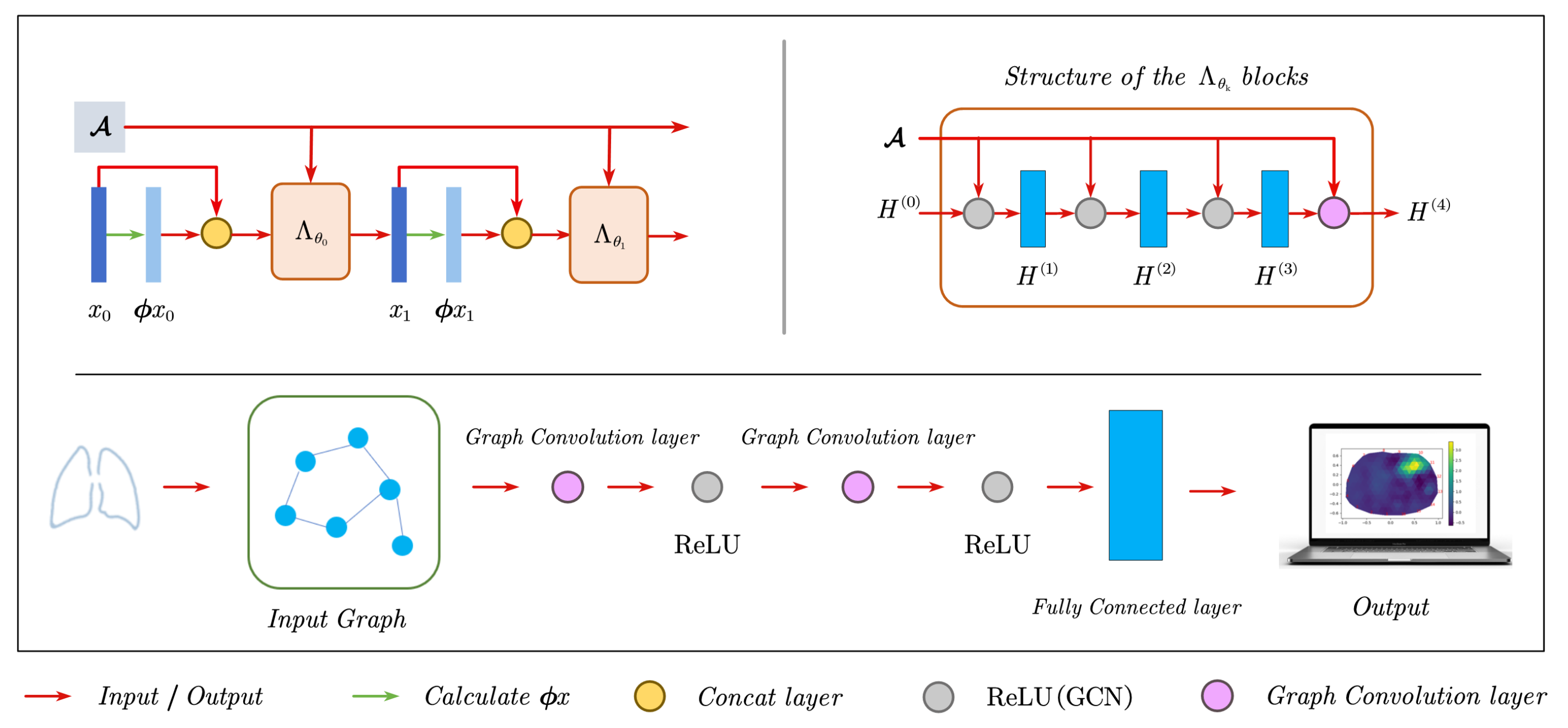
The graph convolution block takes as input the concatenated terms x k and ϕ x k . As seen in Figure 2, the output of the GCN block delivers x k + 1 for the following iteration. In this study, the topology of the network block Λ θ remains constant between iterations; however, each block has a unique set of trainable parameters θ k . We use the LM algorithm in the experiment for iterative solutions without explicit data priors since we want the network to be able to learn features from the training set.
As with previous model-based methods [39,40], there are two alternatives for training the network: end-to-end training of the complete system consisting of k max blocks, or sequential training of each block. Nevertheless, for our scenario, conducting end-to-end training is not feasible because of two primary factors. Initially, performing back-propagation through the updates ϕ x k would be necessary to update the network parameters. To carry out plagiarism checking, adjustments can be made to the text to avoid consecutive identical words. Firstly, it is not possible to compute these updates by assessing the model equations using a FEM solver. Secondly, the evaluation of the model equations consumes a considerable amount of time and leads to extensive training periods. Hence, our approach is to adopt a sequential training method where each block is trained separately. In order to achieve this, a loss function is utilized that necessitates iterative-based optimality. This function is applied to a training set containing pairs of true x t , ( i ) and current iterate x k , ( i ) for i ranging from 1 to N.
Loss θ k = 1 N i = 1 N Λ θ k x k , ϕ x k , A ( i ) x t , ( i ) 2
To evaluate the duplication of a given text, the assessment involves analyzing a quantity x on a finite element method (FEM) mesh consisting of M elements and updating δ x . To ensure plagiarism detection, we must consider two vital elements in this evaluation: an adjacency matrix and a feature matrix. The feature matrix, denoted as H R M × f , primarily comprises rows that correspond to the nodes of the graph, while the columns embody the features defined across these nodes. On the other hand, the adjacency matrix, denoted as A R M × M , is a sparsely populated matrix that depicts the interconnectedness of graph nodes. Only the non-zero entries A i j = 1 indicate the connectivity between graph nodes i and j. In the given context, every component of the network functions as a node in the graph, and two components are deemed linked if they possess at least one shared mesh node. Alternatively, employing the FEM nodes as the graph nodes would be the most suitable selection if the resolution is established at that level.
The problem domain is divided into a discrete FEM, where each element represents a specific region. These elements consist of nodes, discrete points within the region. To extract relevant features from the FEM solution, we consider various factors such as node values, element properties, boundary conditions, and material properties. These features are then used as input for the GNN. The architecture of the network is designed by specifying the number of layers, the type of activation function, and how the layers are interconnected. The input layer of the GNN corresponds to the extracted features from the FEM solution, while the output layer corresponds to the desired output or prediction. To train the GNN, we generate a dataset by selecting a set of FEM problems, solving them using an FEM solver, and recording the input–output pairs. The input consists of the extracted features, while the output represents the desired solution or prediction. The training process involves feeding the input–output pairs to the network, calculating the loss or error between the predicted output and the desired output, and optimizing network parameters using techniques such as back-propagation and gradient descent. Once the network is trained, its performance is evaluated on a separate validation or test dataset. Finally, the trained network can be used to predict the output or solution of a new FEM problem by providing the extracted features as input to the network.

4. Method

We present a groundbreaking strategy to enhance the excellence of EIT imagery by implementing a pioneering algorithm for EIT reconstruction. Initially, we employ the FEM to address the forward problem and obtain crucial FEM grid data. Subsequently, these data are transformed into a network graph within the framework of the GCNM model. To tackle the ill-conditioned non-linear inverse problem in EIT, we employ the improved Newtonian LM method to update the parameters. Ultimately, the algorithm generates a comprehensive EIT image.

4.1. EIT Inverse Model

The process of reconstructing the EIT image involves the solution of an inverse problem. Its objective is to form an image representing the distribution of resistivity/conductivity within the sensitive field W of the medium. This reconstruction is accomplished by utilizing the measured values of boundary voltage in the sensitive field. Resistance tomography is the established method for EIT and serves as the fundamental imaging technology. In electrical impedance imaging, the primary goal of inverse problem-solving is to extract the model parameters from observational data.
To convert the FEM grid data into graph data, we aim to employ GCNM instead of traditional CNNs.
F ( σ ) = 1 2 Λ ( σ ) V meas 2 + R e g ( σ )
where V meas = V 1 ( 1 ) , , V L ( 1 ) , , V 1 ( M ) , , V L ( M ) T in R M L denotes a vector of measured voltages at each L electrode in a k-linearly independent current pattern, and then, the vector Λ = Λ 1 ( 1 ) ( σ ) , , Λ L ( 1 ) ( σ ) , , Λ 1 ( M ) ( σ ) , , Λ L ( M ) ( σ ) T in R M L represents the simulated voltages obtained from L electrodes. These voltages are generated by applying the same K-current pattern with the conductivity σ . The R e g ( σ ) denotes potential regularization factors.
The best constant conductivity was chosen in the experiment to match the data for the first assumption σ 0 . Then, Equation (6) may be changed to
F σ 0 + ϕ σ = 1 2 Λ ( σ + ϕ σ ) V meas 2 + R e g ( σ + ϕ σ )
By solving (7) iteratively, the following update equation is
σ k + 1 = σ k + ϕ σ k
Given an estimate of σ k , this process is iterated until a satisfactory solution is found.

4.1.1. Improved Levenberg–Marquardt Method

LM algorithm has recently been utilized in the adaptation of arbitrarily connected neural (ACN) networks [41]. These ACN networks are capable of tackling more intricate problems while employing fewer neurons [42]. The LM algorithm is particularly effective for minimizing the loss function of the sum of squares error type. As a result, it offers fast training for neural network models that involve this type of error [43]. Implementations of the LM algorithm necessitate the computation of the Jacobian matrix, which is directly related to the total number of training patterns.
Due to its rapid local convergence rates, the LM algorithm and its variations find extensive applications in solving non-smooth equation systems. It proves invaluable in addressing various concerns, including but not limited to non-linear complementarity, variational inequality, Karush–Kuhn–Tucker (KKT) non-linear programming, as well as mechanics and engineering problems [44]. By combining the advantages of stable gradient descent (GD) and the fast convergence near the extreme point of the GN, the LM algorithm overcomes their respective drawbacks. Specifically designed for solving the non-linear inverse problem, the LM method follows a two-step approach, involving the linearization of the non-linear inverse problem and the regularization of the iterative scheme [45].
Our proposed ILM algorithm is improved by the method in [46,47,48]. At the beginning, this method was employed to solve the non-linear least squares multiplication problem [49].
For regular issues of non-linear
F ( x ) = 0
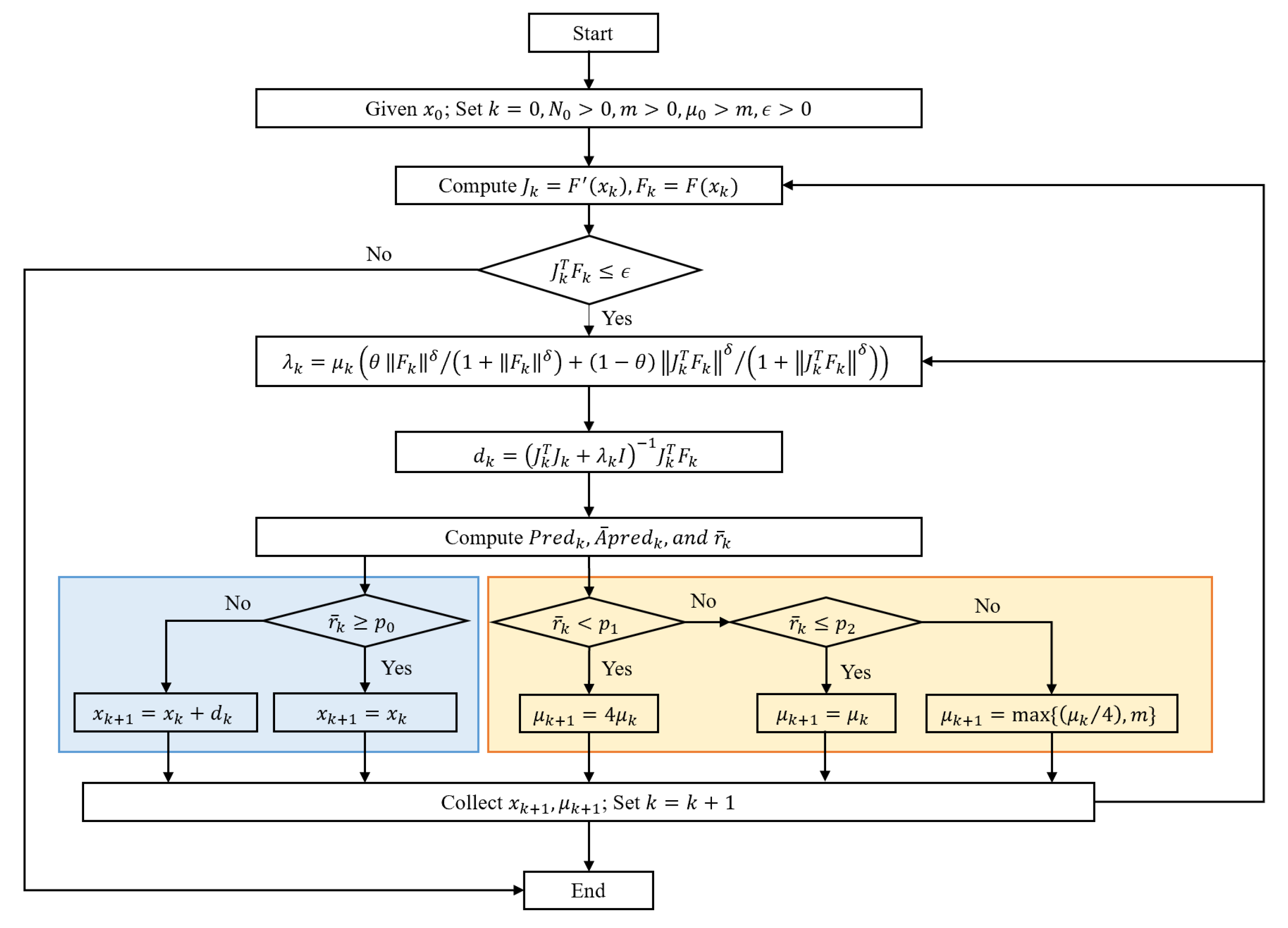
where F ( x ) : R n R m , and the diagram of proposed LM algorithm is shown in Figure 3.
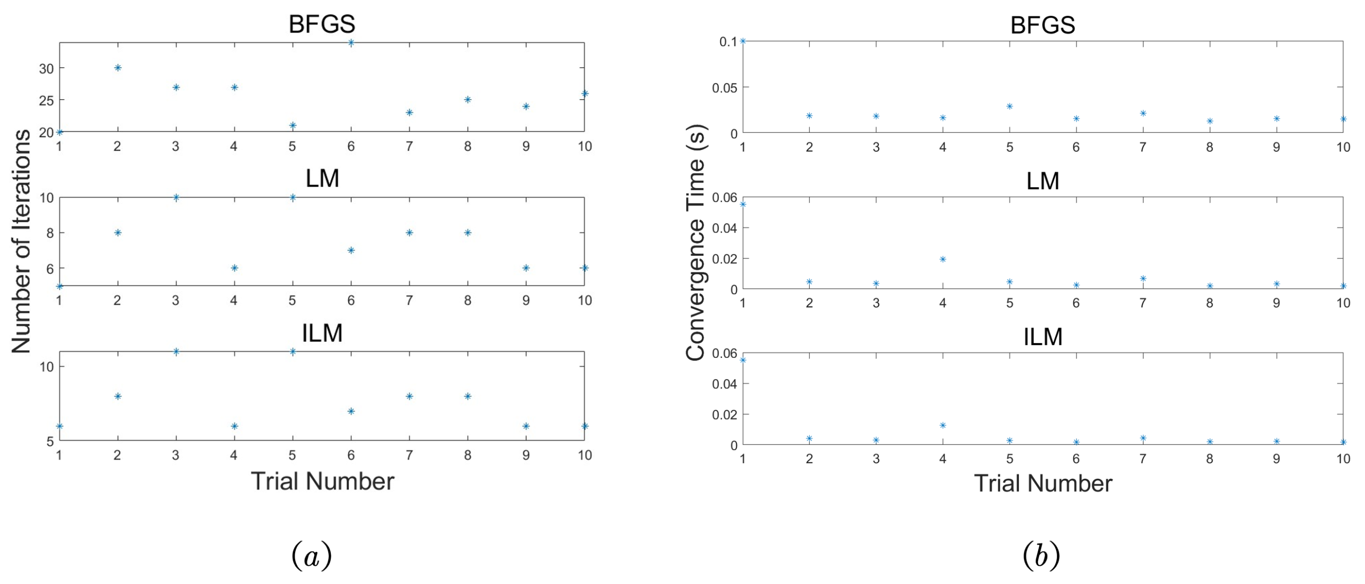
The results obtained from running the Broyden–Fletcher–Goldfarb–Shanno (BFGS), LM, and improved LM algorithms simultaneously are shown in Figure 4. Figure 4a displays the iteration time required to achieve the same termination condition for the objective function value. Figure 4b reveals that the ILM algorithm is similar to the classic LM algorithm in the early iterations but significantly diverges after a certain number of iterations. The ILM algorithm converges each parameter to the target value faster, resulting in faster running speed and significantly fewer iteration steps to reach the same termination condition. In summary, the ILM algorithm provides a search direction closer to the target descent direction, with faster convergence speed and fewer iteration steps.
The following objective function can be minimized in order to generate the inverse EIT problem:
min x X = R n F ( x ) y 2
Assuming that F is Frechet differentiable and denoting its derivative as F ( x ) , the adjoint operator is F ( x ) * , and the algorithm follows a basic form. We start with an initial guess value x 0 X , in the k-th step, let
x k + 1 = x k + d k k = 0 , 1 , x k otherwise
where d k is the result of performing the proposed Newton step.
d k = F x k * F x k + μ k I 1 F x k * y F x k
where μ k > 0 is called the LM parameter. The selection of the parameter μ is the most crucial stage in the LM algorithm.
When the objective function (15) does not contain explicit regularisation, R e g ( σ ) = 0 . The quadratic term of Equation (17) has a Taylor expansion that is given by
F σ 0 + ϕ σ = F ( σ ) + F ( σ ) ( ϕ σ ) + 1 2 F ( σ ) ( ϕ σ ) 2
To facilitate the substitution of GCNs for CNNs in the model-based learning method aimed at addressing non-linear inverse problems, the data represented on the finite element grid are converted into graph data. Graph data consist of nodes connected by edges. This study focuses on undirected, unweighted homogeneous graphs. Graph convolutions, specifically designed for graph data, offer similar advantages as regular CNNs, such as translation variation, localization, and shared weights.
We employ the ILM algorithm to optimize the objective function (7). When the regularization is not explicitly incorporated into the objective function, Equation (8) illustrates the Taylor expansion of the quadratic term of R e g .
F σ 0 + ϕ σ = F ( σ ) + F ( σ ) ( ϕ σ ) + 1 2 F ( σ ) ( ϕ σ ) 2
We can find the minimum value by setting the ϕ σ gradient to 0. We then obtain the updated equation
ϕ σ = F ( σ ) 1 F ( σ )
The gradient and Hessian matrix of the objective function F are denoted by F ( σ ) and F ( σ ) , respectively. It is defined as R e g ( σ ) = 0 when the following two equations hold.
F ( σ ) = J ( σ ) T ( Λ ( σ ) V meas )
F ( σ ) = J ( σ ) T J ( σ ) + i Λ i ( σ ) Λ i ( σ ) V i
The Jacobian matrix of the analog voltage Λ ( σ ) is denoted by J ( σ ) . The Hessian matrix is computed precisely by the Newton technique as Equation (12). However, because of its significant processing cost, the second component in the GN method—which involves calculating the second derivative Λ i ( σ ) —is disregarded. Rather than using this term, the LM algorithm substitutes it with a scaled identity matrix λ ILM I , where the regularization term for ill-posed problems is λ ILM R + . In cases where the rank of the Jacobian matrix is inadequate, this regularization helps increase the condition number of the matrix, which can be found in Equation (16). This method is able to determine the approximate answer to Equation (7).
δ σ I L M = J ( σ ) T J ( σ ) + λ I L M I 1 J ( σ ) T ( λ ( σ ) V meas )
The ILM optimization method obtains an iterative reconstruction algorithm by the update rule (16) and an appropriate stopping criterion.

4.1.2. Regularized Gauss–Newton

To ensure effective plagiarism checks, it is suggested to utilize specific assumptions, such as giving preference to EIT reconstructions with piecewise constant conductivity rather than smooth reconstructions. This objective can be accomplished by utilizing TV with R e g ( σ ) = λ TV i M i σ , where the matrix M represents the discrete gradient in a sparse form [11]. A common practice involves considering a smooth estimation of TV regularization by employing R e g ( σ ) = λ TV i M i σ 2 + ω . The approximated solution for minimizing (8) can then be obtained.
δ σ TV = J ( σ ) T J ( σ ) + λ TV M T E 1 M 1 J ( σ ) T ( U ( σ ) V ) + λ TV M T E 1 M σ
where ω R + represents the smoothing parameter that can be adjusted in order to achieve optimal results. In addition, E = diag ( M σ ) 2 + ω denotes a diagonal matrix. To evaluate the quality of the GCNM reconstructions, we will make a comparison with the TV reconstructions using Equation (20).

4.2. Metrics

Image evaluation indicators encompass a wide range of content and are approached from various perspectives. Each evaluation standard has its own strengths and weaknesses. Full reference image quality evaluation involves selecting an ideal reference image, comparing it with the image to be evaluated, and analyzing the level of distortion in the evaluated image to obtain a quality assessment. Objective evaluation methods for full reference image quality commonly focus on three aspects: pixel statistics, information theory, and structural information. Pixel statistics form the basis for evaluation methods such as peak signal-to-noise ratio ( P S N R ), mean square error ( M S E ), mean absolute error ( M A E ), and signal-to-noise ratio ( S N R ). These methods assess image quality by quantifying the differences in grayscale values between corresponding pixels in the evaluated and reference images. P S N R and M S E specifically measure image quality by calculating the overall magnitude of pixel errors. Higher P S N R values indicate less distortion and better image quality, while lower M S E values indicate better image quality. These methods are straightforward to implement and widely used in areas such as image denoising.
In the field of EIT, the examination of reconstructed images typically encompasses the assessment of image quality and measures of error. In order to observe the resemblance between the reconstructed image and the original image, it is possible to conduct an evaluation of indicators pertaining to image quality by means of visualization. A comparison between the two images allows for the identification of small discrepancies, which suggests a high-quality reconstruction. Two commonly used measurement indicators for image quality are P S N R and S S I M , both of which are significant in assessing the quality of reconstructed images ( P S N R , S S I M ). On the contrary, error indicators enable a numerical assessment of the accuracy of the reconstruction results. M S E and M A E are widely utilized error indicators. While measuring the error output between the reconstructed image and the original image, M S E evaluates the deviation. In contrast, M A E assesses the difference between the actual pixel value and the reconstructed value. Therefore, a comprehensive consideration of these indicators is crucial when evaluating the quality of reconstructed images in EIT ( M S E , M A E ).
We assess the level of variation at the pixel level between the restored image I and the original image K via the M S E defined as
M S E = 1 m n i = 0 m 1 j = 0 n 1 [ I ( i , j ) K ( i , j ) ] 2
The M S E value is calculated based on the total number of pixels in images I and K, denoted as M and N, respectively. A smaller M S E value indicates a higher similarity between the images.
The P S N R , which denotes the ratio between the maximum power of a signal and the power of noise that negatively impacts its accuracy in representation, is an engineering term. To assess P S N R , logarithmic decibel units are often employed, owing to the extensive dynamic ranges exhibited by numerous signals.
P S N R = 10 · log 10 L 2 M S E
L is a constant denoting the maximum dynamic range of the image data type, signifying the upper limit of the value range. For instance, in the case of image data represented by the float type, where the value range lies between 0 and 1, L is assigned a value of 1. Conversely, for image data representing uint-8 type, where the value range spans from 0 to 255, L takes the value of 255. The P S N R formula presents MSE in the denominator, implying that a higher P S N R value indicates superior image quality during evaluation, contrary to M S E ’s interpretation.
The S S I M index is a widely employed measure for quantifying the resemblance of two images. To directly evaluate meshes, the S S I M index has been appropriately adapted. The range of the S S I M value extends from 0 to 1, with a greater value denoting a lesser disparity between the output image and the undistorted image, thereby signifying superior image quality. The calculation of S S I M relies on three comparative metrics pertaining to the samples α and β —luminance, contrast, and structure.
l ( α , β ) = 2 μ α μ β + c 1 μ α 2 + μ β 2 + c 1 , c ( α , β ) = 2 σ α σ β + c 2 σ α 2 + σ β 2 + c 2 , s ( α , β ) = σ α β + c 3 σ α σ β + c 3
where μ α and μ β are the average of α and β . σ α 2 and σ β 2 are the variance of α and β . σ α β is the covariance of α and β . The calculation formula of S S I M is as follows.
S S I M ( α , β ) = l ( α , β ) λ 1 · c ( α , β ) λ 2 · s ( α , β ) λ 3
The proportion of different features in S S I M measurement is typically represented by λ 1 , λ 2 , λ 3 . To avoid instability problems caused when the denominator is 0, we introduce three constants: C 1 , C 2 , C 3 . It is common to take λ 1 = λ 2 = λ 3 = 1 , and then C 2 = C 3 / 2 , so we can obtain
S S I M ( α , β ) = 2 μ x μ β + C 1 2 σ α β + C 2 μ α 2 + μ β 2 + C 1 σ x 2 + σ β 2 + C 2
where C 1 = K 1 L 2 and C 2 = K 2 L 2 .

5. Experiment and Analysis

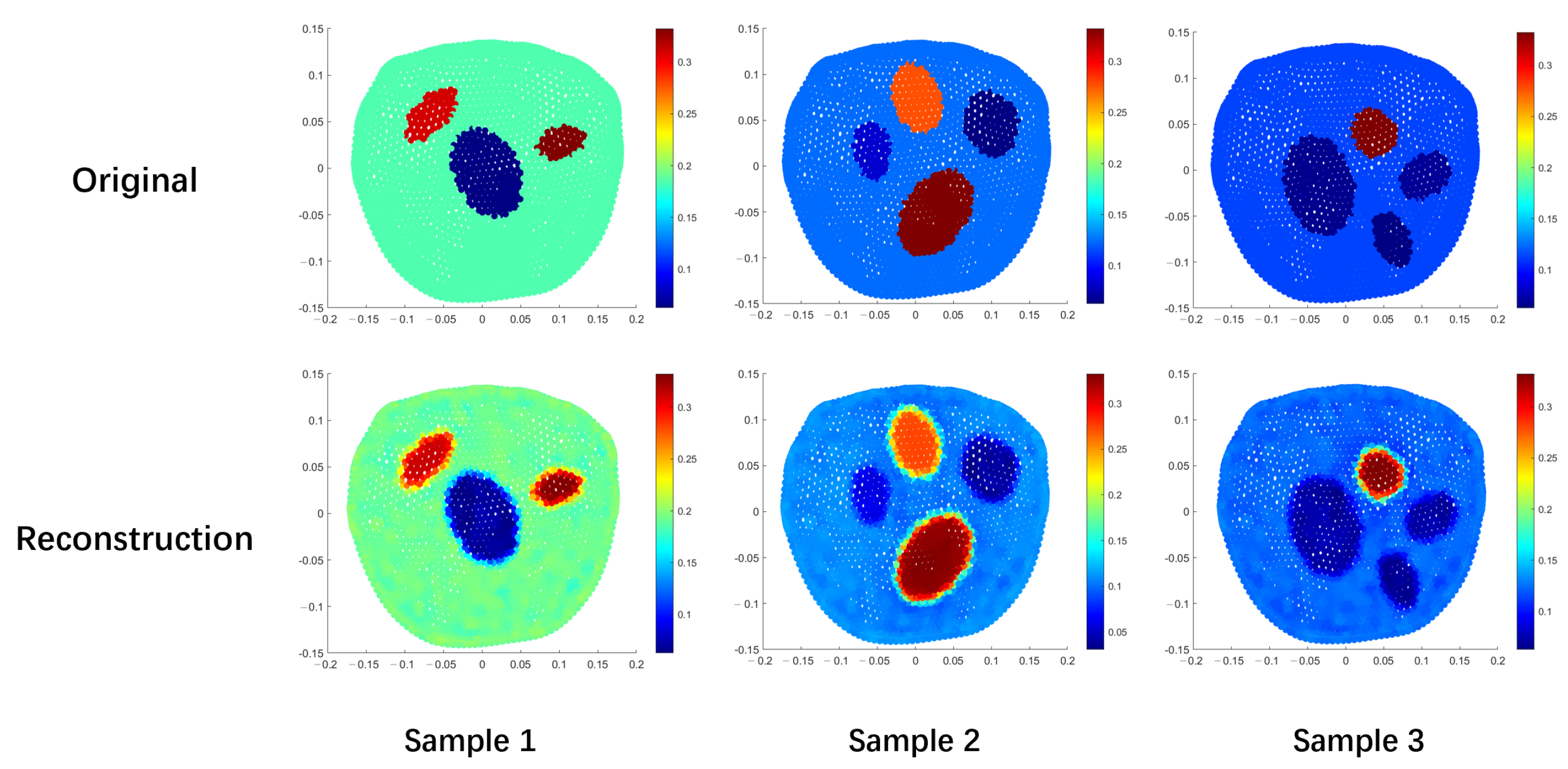
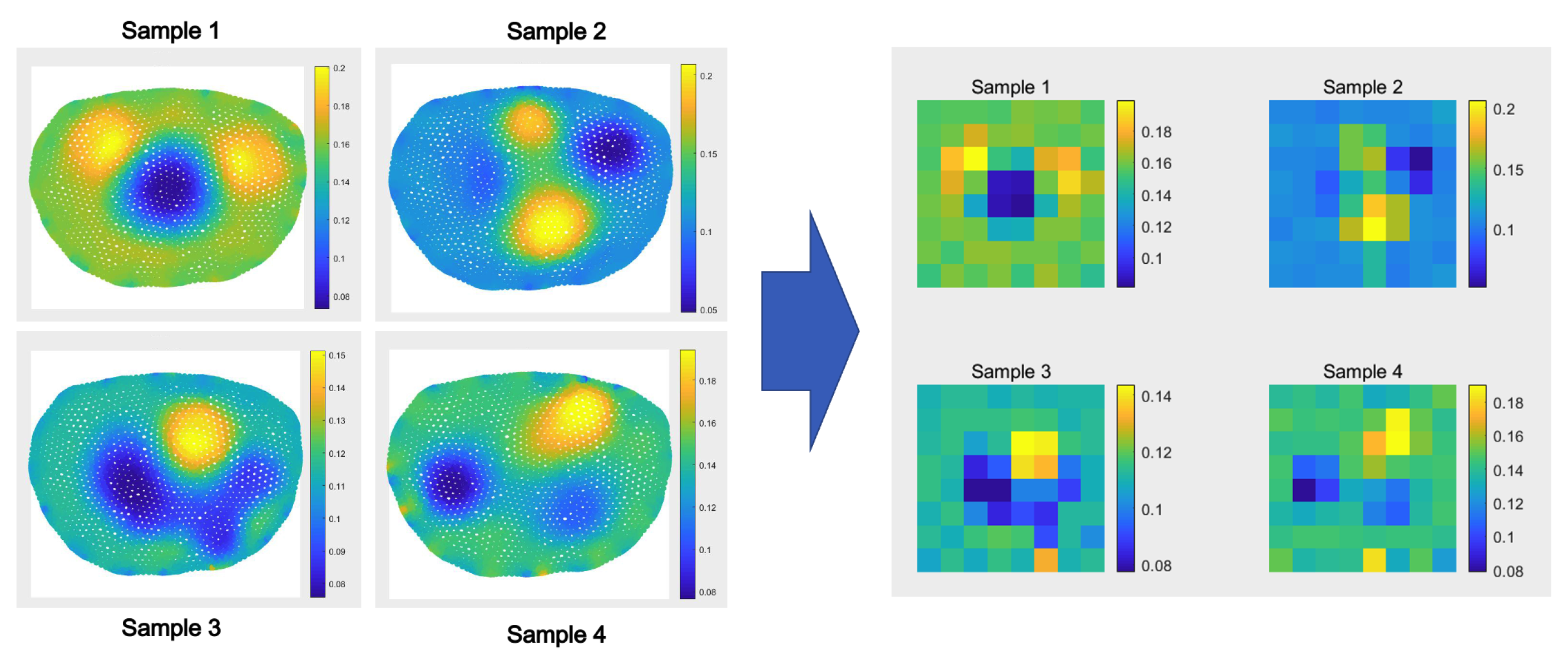
First, we use simulated data to visually test the quality of the GNN method. The experiment used Python version 3.8, PyTorch version 1.13, and EIDORS version 3.10. The simulated data include 200 training and 100 test samples, as shown in Figure 5. Each simulated model contains 1–4 ellipses with constant resistivity. The model defines these ellipses on the same circular grid with a radius of 140 mm. The circular grid consists of 32 electrodes, each with a width and height of 20 mm, placed at equal intervals. The excitation mode used in the experiment is the adjacent current mode of 2 mA.
The data collected for this study come from two different systems: the 32-electrode ACT 3 system and the 16-electrode KIT 4 system [50]. The ACT 3 system utilized a triangular current mode with a maximum amplitude of 0.2 mA and a frequency of 28.8 kHz. The electrodes are uniformly distributed, with a width of 25 mm and a salt height of 16 mm, placed in grooves with a radius of 150 mm. The KIT 4 system, on the other hand, used neighboring current patterns with amplitudes of 3 mA and frequencies of 10 kHz. The circular tank utilized in this system had a radius of 140 mm, and the electrodes were about center, with a width of 25 mm. The tank contained two targets—a large resistor with a conductivity of 0.067 S/m and a small conductor with a conductivity of 0.305 S/m. We placed the target at a height of 45 mm in the salt bath. A chest-shaped slot with a circumference of 1020 mm and an electrode width of 20 mm was used.
The reconstructed results of the simulated data are presented in Figure 5, while the evaluation index results can be found in Table 1.
In this experiment, we use the finite element method to solve a direct EIT problem with approximately 5000 triangular elements. The raster data are on the left side of the Figure 6. In addition, we do not investigate the effect of mesh granularity on the accuracy of different reconstruction techniques. Before training the model, the resulting finite element mesh data must be converted to the graph data format required for neural convolutional graphs.
Our work employs the control variable method to compare the results of multiple experiments. The selected parameters for the experiment include λ L M = 0.1 and a convolutional network with a depth of 2 to train the model. The implementation in PyTorch utilizes a mini-batch of 512 samples. It combines the optimization methods of Adam [51] and limited memory Broyden–Fletcher–Goldfarb–Shanno (LBFGS) [52] to perform minimization training of the iterative loss function for each block. The learning rate is 0.002. Training ends if the validation loss for 100 epochs does not decrease, and the minimum validation loss for the trainable parameters remains unchanged.
We simulated static EIT without noise interference. The simulation results were obtained by performing computer numerical calculations, using theoretical voltage data with minimal error. However, noise inevitably influences measurement data, including power frequency interference in practical applications such EIT and other fields. Despite efforts to reduce these interferences through hardware circuits, eliminating them remains challenging.
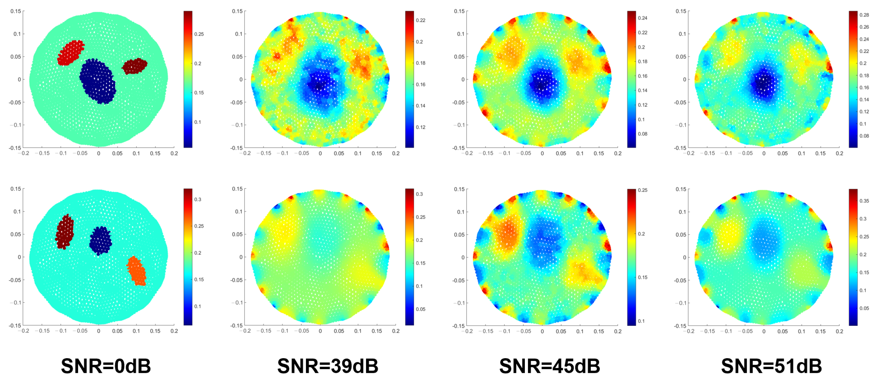
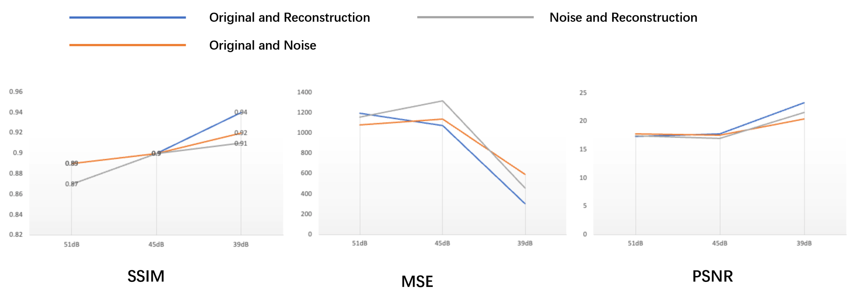
This experiment examines the anti-noise performance of the Newton-based GCN by adding Gaussian noise to the simulated data. Specifically, Gaussian noise with signal-to-noise ratios of 0 dB, 39 dB, 45 dB, and 51 dB is added when calculating the voltage data on adjacent electrodes. These four values cover a wide range of SNR conditions, ranging from very low (0 dB) to very high (51 dB). They can be used to evaluate the performance of the system under different SNR conditions [53]. The Newton-based GCNM algorithm is then used to reconstruct the static image. The reconstructed images under different SNR conditions are compared with the noise-free reconstructed image to analyze the anti-noise performance. Figure 7 displays the reconstructed images at different SNR levels.
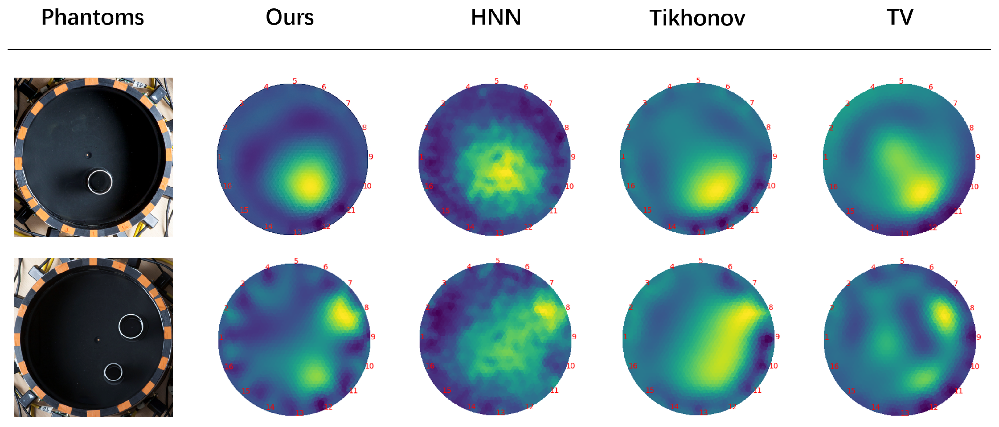
Finally, we have tested the proposed algorithm on real data and illustrated the reconstruction performance, as shown in Figure 8.

6. Discussion

The results of this study indicate that the proposed algorithm has a good performance. To further evaluate the performance of the algorithm, we conducted a flume experiment using the proposed imaging algorithm in Figure 9. The flume data were obtained from the EIT system KIT 4, developed by the University of Eastern Finland. The KIT 4 system is an open EIT system that generates a two-dimensional EIT dataset. These data were not included in the training and test sets used in this article. The KIT 4 system provides a circular tank with a radius of 14 cm, equipped with 16 rectangular stainless steel electrodes evenly spaced around the tank wall. Each electrode has a width of 2.5 cm. Physiological saline was used as the filler in the tank to create the background field. The system utilizes an excitation current size of 2 mA and a frequency of 1 kHz, with a proximity drive mode. The obtained data were processed and converted into the pyEIT format.
Based on the data presented in Table 2, it is evident that our algorithm outperforms the other methods in terms of the S S I M and M S E evaluation indicators while ranking second in terms of P S N R . Although artifacts are present in the reconstructed images produced by all three methods, the artifacts are most effectively reduced in the reconstructed images generated by the proposed algorithm. It is important to note that actual measurements are subject to measurement errors, model errors, and environmental noise interference, which result in a reduced signal-to-noise ratio of the measured voltage. Consequently, the quality of the actual reconstructed image is lower than that of the simulated calculation. This further supports the conclusion that our alogrithm offers superior imaging quality.
We contribute to the research on lung EIT imaging algorithms by conducting simulation experiments and experiments with ACT 3 and KIT 4 datasets to verify the effectiveness of the proposed improved GNN algorithm. However, further optimization of the algorithm is still necessary due to experimental conditions. There is potential for additional research and improvement. To facilitate observation and verification of imaging results, a circular field is used instead of a chest model to construct the EIT simulation model. However, since there are notable differences in shape and size between the human chest contour and the circular field, distortion of the reconstructed image may occur when applying the algorithm in practical lung imaging.

7. Conclusions

The paper introduces a novel approach for electrical impedance imaging by combining the convolution graph neural network and LM connection method. This method leverages Newton’s neural network convolution graph to effectively address non-linear issues. The numerical experiments conducted underscore the success of GN graph convolution, despite some constraints in depicting intricacies. Moreover, the proposed technique demonstrates promising viability in attending to practical non-linear inverse functions. In the forthcoming research, our objective is to refine our proposed method and devise new architectures that will augment the excellence of EIT reconstruction images and optimize processing speed.
EIT is undeniably an invaluable tool for diagnosing pulmonary issues in the future, particularly for patients in the ICU who require constant monitoring. The convenience and bedside applicability of EIT make it especially beneficial in this setting.

Author Contributions

Conceptualization, R.Z. and C.X.; methodology, R.Z.; software, R.Z. and W.M.; validation, R.Z.; investigation, Z.Z.; resources, Z.Z. and W.M.; data curation, R.Z.; writing—original draft preparation, R.Z.; writing—review and editing, R.Z.; visualization, R.Z.; supervision, C.X. and W.M.; project administration, C.X.; funding acquisition, R.Z., C.X., Z.Z. and W.M. All authors have read and agreed to the published version of the manuscript.

Funding

This work is supported by the National Natural Science Foundation of China (61967004, 11901137, 11961011, 72061007, 62171147), the Guangxi Key Laboratory of Cryptography and Information Security (GCIS201927), and the Guangxi Key Laboratory of Automatic Detecting Technology and Instruments (YQ20113, YQ20114, YQ23015).

Institutional Review Board Statement

Not applicable.

Informed Consent Statement

Not applicable.

Data Availability Statement

The data that support the findings of this study will be available from the corresponding author upon reasonable request. The data are not publicly available due to privacy.

Conflicts of Interest

The authors declare no conflicts of interest and the funders had no role in the design of the study.

References

  1. Adler, A.; Boyle, A. Electrical impedance tomography: Tissue Properties to image measures. IEEE Trans. Biomed. Eng. 2017, 64, 2494–2504. [Google Scholar] [CrossRef]
  2. Benning, M.; Burger, M. Modern regularization methods for inverse problems. Acta Numer. 2018, 27, 1–111. [Google Scholar] [CrossRef]
  3. Adler, J.; Öktem, O. Solving ill-posed inverse problems using iterative deep neural networks. Inverse Probl. 2017, 33, 124007. [Google Scholar] [CrossRef]
  4. Harikumar, R.; Prabu, R.; Raghavan, S. Electrical impedance tomography (EIT) and its medical applications: A review. Int. J. Soft Comput. Eng 2013, 3, 193–198. [Google Scholar]
  5. Jiang, Y.D.; Soleimani, M. Capacitively Coupled Electrical Impedance Tomography for Brain Imaging. IEEE Trans. Med. Imaging 2019, 38, 2104–2113. [Google Scholar] [CrossRef] [PubMed]
  6. Bader, O.; Hafsa, M.; Amara, N.E.B.; Kanoun, O. Two-dimensional forward modeling for human thorax imaging based on electrical impedance tomography. In Proceedings of the 2021 International Workshop on Impedance Spectroscopy (IWIS), Chemnitz, Germany, 29 September–1 October 2021; IEEE: Piscataway, NJ, USA, 2021; pp. 114–117. [Google Scholar]
  7. Xu, C.; Dong, X. Advancements in electrical impedance tomography and its clinical applications. High Volt. Eng. 2014, 40, 3738–3745. [Google Scholar]
  8. Dong, Q.; Zhang, Y.; He, Q.; Xu, C.; Pan, X. Image reconstruction method for electrical impedance tomography based on RBF and attention mechanism. Comput. Electr. Eng. 2023, 110, 108826. [Google Scholar] [CrossRef]
  9. Hrabuska, R.; Prauzek, M.; Venclikova, M.; Konecny, J. Image reconstruction for electrical impedance tomography: Experimental comparison of radial basis neural network and Gauss–Newton method. IFAC-PapersOnLine 2018, 51, 438–443. [Google Scholar] [CrossRef]
  10. Vauhkonen, M.; Vadász, D.; Karjalainen, P.A.; Somersalo, E.; Kaipio, J.P. Tikhonov regularization and prior information in electrical impedance tomography. IEEE Trans. Med. Imaging 1998, 17, 285–293. [Google Scholar] [CrossRef]
  11. Borsic, A.; Graham, B.M.; Adler, A.; Lionheart, W.R. In vivo impedance imaging with total variation regularization. IEEE Trans. Med. Imaging 2009, 29, 44–54. [Google Scholar] [CrossRef]
  12. Chandrasekaran, V.; Recht, B.; Parrilo, P.A.; Willsky, A.S. The convex geometry of linear inverse problems. Found. Comput. Math. 2012, 12, 805–849. [Google Scholar] [CrossRef]
  13. Xu, Y.; Pei, Y.; Dong, F. An adaptive Tikhonov regularization parameter choice method for electrical resistance tomography. Flow Meas. Instrum. 2016, 50, 1–12. [Google Scholar] [CrossRef]
  14. Xu, Z.; Yang, Y.; Sun, J. A new approach to solve inverse problems: Combination of model-based solving and example-based learning. Sci. Sin. (Math.) 2017, 47, 1345–1354. [Google Scholar]
  15. Chen, Z.; Ma, G.; Jiang, Y.; Wang, B.; Soleimani, M. Application of deep neural network to the reconstruction of two-phase material imaging by capacitively coupled electrical resistance tomography. Electronics 2021, 10, 1058. [Google Scholar] [CrossRef]
  16. Kong, L.; Bin, G.; Wu, S. Comparative study on reconstruction methods of electrical impedance tomography. China Med. Devices 2022, 37, 1–9. [Google Scholar]
  17. Martins, T.D.C.; Sato, A.K.; Moura, F.S.D.; de Camargo, E.D.L.B.; Tsuzuki, M.D.S.G. A Review of Electrical Impedance Tomography in Lung Applications: Theory and Algorithms for Absolute Images. Annu. Rev. Control 2019, 48, 442–471. [Google Scholar] [CrossRef]
  18. Adler, A.; Arnold, J.H.; Bayford, R.; Borsic, A.; Brown, B.; Dixon, P.; Faes, T.J.; Frerichs, I.; Gagnon, H.; Gärber, Y.; et al. GREIT: A unified approach to 2D linear EIT reconstruction of lung images. Physiol. Meas. 2009, 30, S35. [Google Scholar] [CrossRef]
  19. Guo, R.; Jiang, J. Construct Deep Neural Networks based on Direct Sampling Methods for Solving Electrical Impedance Tomography. SIAM J. Sci. Comput. 2021, 43, B678–B711. [Google Scholar] [CrossRef]
  20. Liu, S.; Jia, J.; Zhang, Y.D.; Yang, Y. Image reconstruction in electrical impedance tomography based on structure-aware sparse Bayesian learning. IEEE Trans. Med. Imaging 2018, 37, 2090–2102. [Google Scholar] [CrossRef]
  21. Herzberg, W.; Rowe, D.B.; Hauptmann, A.; Hamilton, S.J. Graph convolutional networks for model-based learning in nonlinear inverse problems. IEEE Trans. Comput. Imaging 2021, 7, 1341–1353. [Google Scholar] [CrossRef]
  22. Seo, J.K.; Kim, K.C.; Jargal, A.; Lee, K.; Harrach, B. A Learning-Based Method for Solving Ill-Posed Nonlinear Inverse Problems: A Simulation Study of Lung EIT. SIAM J. Imaging Sci. 2019, 12, 1275–1295. [Google Scholar] [CrossRef]
  23. Jauhiainen, J.; Kuusela, P.; Seppanen, A.; Valkonen, T. Relaxed Gauss–Newton methods with applications to electrical impedance tomography. SIAM J. Imaging Sci. 2020, 13, 1415–1445. [Google Scholar] [CrossRef]
  24. Liu, Z.; Yang, Y. Multimodal Image Reconstruction of Electrical Impedance Tomography Using Kernel Method. IEEE Trans. Instrum. Meas. 2022, 71, 1–12. [Google Scholar] [CrossRef]
  25. Bayford, R.H. Bioimpedance tomography (electrical impedance tomography). Annu. Rev. Biomed. Eng. 2006, 8, 63–91. [Google Scholar] [CrossRef] [PubMed]
  26. Fessler, J.A. Model-based image reconstruction for MRI. IEEE Signal Process. Mag. 2010, 27, 81–89. [Google Scholar] [CrossRef]
  27. Sun, B.; Zhong, H.; Zhao, Y.; Ma, L.; Wang, H. Calderón’s Method-Guided Deep Neural Network for Electrical Impedance Tomography. IEEE Trans. Instrum. Meas. 2023, 72, 1–11. [Google Scholar] [CrossRef]
  28. Fan, Y.; Ying, L. Solving electrical impedance tomography with deep learning. J. Comput. Phys. 2020, 404, 109119. [Google Scholar] [CrossRef]
  29. Zong, Z.; Wang, Y.; Wei, Z. A review of algorithms and hardware implementations in electrical impedance tomography. Prog. Electromagn. Res. 2020, 169, 59–71. [Google Scholar] [CrossRef]
  30. Newell, J.; Isaacson, D.; Mueller, J. Electrical Impedance Tomography. IEEE Trans. Med. Imaging 2002, 21, 553–554. [Google Scholar] [CrossRef]
  31. Gernandt, H.; Rohleder, J. A Calderón type inverse problem for tree graphs. Linear Algebra Its Appl. 2022, 646, 29–42. [Google Scholar] [CrossRef]
  32. Jin, B.; Khan, T.R.; Maass, P. A reconstruction algorithm for electrical impedance tomography based on sparsity regularization. Int. J. Numer. Methods Eng. 2012, 89, 337–353. [Google Scholar] [CrossRef]
  33. Adler, A.; Lionheart, W.R.B. Uses and abuses of EIDORS: An extensible software base for EIT. Physiol. Meas. 2006, 27, S25–S42. [Google Scholar] [CrossRef] [PubMed]
  34. Kipf, T.N.; Welling, M. Semi-Supervised Classification with Graph Convolutional Networks. arXiv 2016, arXiv:1609.02907. [Google Scholar]
  35. Zhou, J.; Cui, G.; Hu, S.; Zhang, Z.; Yang, C.; Liu, Z.; Wang, L.; Li, C.; Sun, M. Graph neural networks: A review of methods and applications. AI Open 2020, 1, 57–81. [Google Scholar] [CrossRef]
  36. Wu, Z.; Pan, S.; Chen, F.; Long, G.; Zhang, C.; Yu, P.S. A Comprehensive Survey on Graph Neural Networks. IEEE Trans. Neural Netw. Learn. Syst. 2021, 32, 4–24. [Google Scholar] [CrossRef] [PubMed]
  37. Lucas, A.; Iliadis, M.; Molina, R.; Katsaggelos, A.K. Using deep neural networks for inverse problems in imaging: Beyond analytical methods. IEEE Signal Process. Mag. 2018, 35, 20–36. [Google Scholar] [CrossRef]
  38. Gulakala, R.; Markert, B.; Stoffel, M. Graph Neural Network enhanced Finite Element modelling. PAMM 2023, 22, e202200306. [Google Scholar] [CrossRef]
  39. Seifnaraghi, N.; De Gelidi, S.; Nordebo, S.; Kallio, M.; Frerichs, I.; Tizzard, A.; Suo-Palosaari, M.; Sophocleous, L.; van Kaam, A.H.; Sorantin, E.; et al. Model selection based algorithm in neonatal chest EIT. IEEE Trans. Biomed. Eng. 2021, 68, 2752–2763. [Google Scholar] [CrossRef]
  40. Proença, M.; Braun, F.; Solà, J.; Thiran, J.P.; Lemay, M. Noninvasive pulmonary artery pressure monitoring by EIT: A model-based feasibility study. Med. Biol. Eng. Comput. 2017, 55, 949–963. [Google Scholar] [CrossRef]
  41. Fan, J. Accelerating the modified Levenberg-Marquardt method for nonlinear equations. Math. Comput. 2014, 83, 1173–1187. [Google Scholar] [CrossRef]
  42. Wilamowski, B.M.; Yu, H. Improved Computation for Levenberg–Marquardt Training. IEEE Trans. Neural Netw. 2010, 21, 930–937. [Google Scholar] [CrossRef]
  43. Luo, X.L.; Liao, L.Z.; Wah Tam, H. Convergence analysis of the Levenberg–Marquardt method. Optim. Methods Softw. 2007, 22, 659–678. [Google Scholar] [CrossRef]
  44. Fan, J.; Huang, J.; Pan, J. An adaptive multi-step Levenberg–Marquardt method. J. Sci. Comput. 2019, 78, 531–548. [Google Scholar] [CrossRef]
  45. Fu, X.; Li, S.; Fairbank, M.; Wunsch, D.C.; Alonso, E. Training recurrent neural networks with the Levenberg–Marquardt algorithm for optimal control of a grid-connected converter. IEEE Trans. Neural Netw. Learn. Syst. 2014, 26, 1900–1912. [Google Scholar] [CrossRef] [PubMed]
  46. Huang, B.; Ma, C. The Modulus-Based Levenberg-Marquardt Method for Solving Linear Complementarity Problem. Numer. Math. Theory Methods Appl. 2019, 12, 154–168. [Google Scholar]
  47. Zhang, R.; Yang, H. A Discretizing Levenberg-Marquardt Scheme for Solving Nonlinear Ill-Posed Integral Equations. J. Comput. Math. 2022, 40, 686–710. [Google Scholar] [CrossRef]
  48. Fan, J. The modified levenberg-marquardt method for nonlinear equations with cubic convergence. Math. Comput. 2012, 81, 447–466. [Google Scholar] [CrossRef]
  49. Fan, J.y. A modified Levenberg-Marquardt algorithm for singular system of nonlinear equations. J. Comput. Math. 2003, 21, 625–636. [Google Scholar]
  50. Hamilton, S.J.; Mueller, J.; Santos, T. Robust computation in 2D absolute EIT (a-EIT) using D-bar methods with the ‘exp’approximation. Physiol. Meas. 2018, 39, 064005. [Google Scholar] [CrossRef]
  51. Haji, S.H.; Abdulazeez, A.M. Comparison of optimization techniques based on gradient descent algorithm: A review. PalArch’s J. Archaeol. Egypt/Egyptol. 2021, 18, 2715–2743. [Google Scholar]
  52. Bollapragada, R.; Nocedal, J.; Mudigere, D.; Shi, H.J.; Tang, P.T.P. A progressive batching L-BFGS method for machine learning. In Proceedings of the International Conference on Machine Learning, Stockholm, Sweden, 10–15 July 2018; pp. 620–629. [Google Scholar]
  53. Fan, L.; Zhang, F.; Fan, H.; Zhang, C. Brief review of image denoising techniques. Vis. Comput. Ind. Biomed. Art 2019, 2, 7. [Google Scholar] [CrossRef] [PubMed]
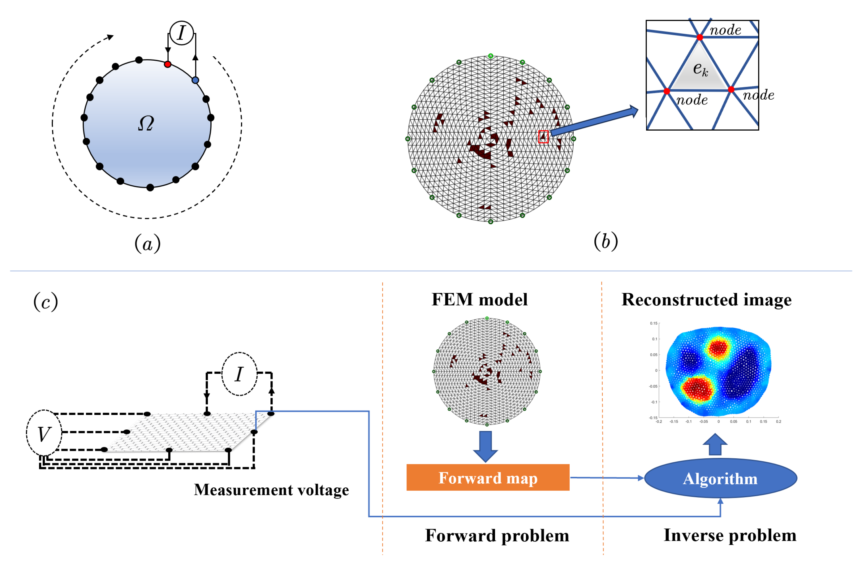
Figure 1. The principle of EIT. (a) The basic working principle of EIT involves taking voltage measurements at every electrode for each current injection. (b) Diagram illustrating the subdivision of finite elements on a 2D circular domain. (c) Typical schematic of forward and inverse problems in EIT.
Applsci 14 00595 g001
Figure 2. Graph convolution structure based on Newton’s method. The initial two iterations of GCNM are depicted in the top left. An individual block within the network is illustrated in the top right, where Λ θ represents a NN with parameters θ . Both GCNM and GResNet utilize the same block structure. In the GCNM, the input H ( 0 ) is created by concatenating x k and ϕ x k , while the output H ( 0 ) corresponds to x ( k + 1 ) . In GResNet, H ( 0 ) represents x 1 in the first block, and in the subsequent blocks, it represents the sum of the input and output from the previous block. The bottom part showcases GResNet, which includes the first iteration of a traditional Newton method as input in the first block, followed by a total of k max blocks.
Applsci 14 00595 g002
Figure 3. The diagram of the ILM algorithm.
Applsci 14 00595 g003
Figure 4. Iterations for each parameter value obtained by running the three algorithms simultaneously once. (a) Number of iterations for each algorithm. (b) Average computation times for each algorithm.
Applsci 14 00595 g004
Figure 5. Some simulation samples.
Applsci 14 00595 g005
Figure 6. Transformation of finite element mesh data into graph structure.
Applsci 14 00595 g006
Figure 7. The effect of the reconstructed image under different SNR. The simulated test data results were obtained using a network trained on ACT 4 data. It is important to note that the training data only include a single horizontal segmentation of the lungs.
Applsci 14 00595 g007
Figure 8. The S S I M , M S E , and P S N R values of reconstruction methods under different S N R .
Applsci 14 00595 g008
Figure 9. Physical model imaging of a circular sink with acrylic cylinders.
Applsci 14 00595 g009
Table 1. Evaluation metrics for simulated data.
Sample 1Sample 2Sample 3
MSE155.01438.20361.47
PSNR26.2321.7122.55
SSIM0.970.930.94
Table 2. Evaluation indexes of tank experiments.
MSEPSNRSSIM
Ours1314.3634.77550.8658
HNN938.5633.95520.8398
Tikhonov1073.8034.22600.8509
TV1138.5634.09330.8465
Ours1179.7433.90580.8594
HNN589.6233.87480.84590
Tikhonov1081.0434.01210.8444
TV1156.3133.88600.8557
Disclaimer/Publisher’s Note: The statements, opinions and data contained in all publications are solely those of the individual author(s) and contributor(s) and not of MDPI and/or the editor(s). MDPI and/or the editor(s) disclaim responsibility for any injury to people or property resulting from any ideas, methods, instructions or products referred to in the content.