1. Introduction
The evolution of lead-free solder alloys, particularly in the context of electronic manufacturing, represents a significant shift in material science and engineering. While the use of soldering for mechanical and electrical connections has a long history, recent advancements have been driven by the need for environmentally friendly and high-performance alternatives to traditional tin–lead (Sn-Pb) solders. Soldering electronic components together using ‘soft soldering’, which involves much lower temperatures, is a much more recent development.
Early soft soldering employed pure tin. Alloys were created over time to solve challenges such as thermal cycling, shock tolerance, electron migration, and whisker formation in tin-based alloys [
1]. Although lead could play this role in most soldering applications, the elimination of lead from devices and the implementation of new standards for more fine-pitched parts necessitated the development of new solder alloys. To be considered a viable alternative to Sn-Pb solders, lead-free candidates must offer qualities and functionality comparable to or greater than those of eutectic or close eutectic Sn-Pb solders. The presence of Pb in solders improves the overall efficiency of the Sn-Pb solder.
In addition to carrying electricity, solder joints provide mechanical support for electrical devices. As a result, the mechanical qualities of solder alloys are critical in the production of long-lasting products. Tensile characteristics and creep are particularly important for evaluating the mechanical properties of solders and have consequently been widely researched [
2]. SAC is an abbreviation for the alloy SnAgCu (tin, silver, and copper). SAC alloys are the most widely utilised alloys in the electronics industry. SAC305, a lead-free grade alloy, is made up of 96.5% tin, 3% silver, and 0.5% copper. Its 3% silver component ensures optimum wetting qualities as well as balanced thermal fatigue, solder link power, and mechanical stress resistance [
3]. Solder pastes are made up of a metal alloy powder (about 90% by weight) and a cream-like organic chemical component (approximately 10% by weight). ‘Flux’, the cream of organic components, is usually a trade secret or patent-protected [
4]. This study aims to delve deeper into the mechanical behaviour of Pb-free solder alloys, specifically their response to different strain rates and constant stresses. A model considering both elastic and plastic deformation along with creep behaviour is being developed to accurately represent the stress–strain characteristics of these alloys [
5,
6].
The mechanical characteristics of lead-free solders, particularly SAC305, are highly dependent on parameters such as temperature and strain rate. This reliance is caused by the high homologous temperature of these solder alloys, which makes comparing results across research difficult. Such disparities are caused by a lack of consistent testing circumstances, which includes differences in specimen preparation processes and strain rates. Despite these difficulties, a broad spectrum of mechanical characteristics has been determined. The elastic modulus of SAC alloys, including SAC305, normally ranges from 30 to 54 GPa, with the majority of values falling between 40 and 50 GPa. In terms of tensile parameters, the Sn-3.9Ag-0.5Cu variation has an elastic modulus of 50.3 GPa, an ultimate tensile strength (UTS) of 54 MPa, and a yield strength (YS) of 36.2 MPa. Variations in these values are observed between research, which can be attributed to the various testing procedures used. As a result, these stated data must be evaluated with caution, taking into account the high heterogeneity due to the various production technologies and conditions [
7].
SACX0807 (Alpha SACX Plus 0807) is a low-silver lead-free alloy intended to give soldering and reliability characteristics equal to those of higher-silver SAC305. Tensile properties and microstructure are compared with SAC305 in [
8]. The corrosion behaviour of SAC305 and SACX0807 under application conditions was correlated with the microstructure of the alloy and the electrochemical behaviour in [
9,
10]. The creep behaviour of SACX0807 has not yet been reported. This is an important gap in the field that should be covered by this work (at room temperature).
With a focus on SAC alloys such as SAC305 or SACX0807, it is necessary to investigate the Strain Rate Sensitivity (SRS) of the material. The peculiar microstructure of this alloy, which includes Sn, Ag3Sn, and Cu6Sn5, has a substantial impact on its mechanical behaviour at varied strain rates. In particular, SAC305 exhibits a decrease in SRS as the temperature and strain rate increase, which is an important element in determining the mechanical stability of solder connections in electronic devices [
11]. This discovery is especially important in operational settings involving dynamic mechanical loads. Understanding these correlations is critical for forecasting solder performance and guaranteeing electronic assembly durability [
12].
The fatigue life of SAC305 under different wave loading situations, as investigated in publications [
13,
14,
15], gives important insights into the solder’s behaviour. By including both plastic and creep strain components, they considerably improve our knowledge of SAC305 fatigue behaviour. Another critical consideration is the effect of ageing on the fatigue life of SAC305 [
16]. The lower mechanical fatigue life due to age, notably in SAC305, shows the importance of a thorough examination of stress relaxation and low cycle fatigue features. A recent study [
5] emphasises the importance of the constitutive viscoplastic model for SAC305 and provides an in-depth look at the ratcheting behaviour of SAC305 under cyclic loading, highlighting its lower time-dependent deformation compared to Sn-37Pb. This difference is due to the distinct microstructural and mechanical characteristics of SAC305, which emphasises the exceptional capacity of the material to carry cyclic loads. This is critical for the dependability of mechanically stressed electronic systems.
Some authors of the paper developed a special experimental technique based on the Digital Image Correlation (DIC) method, which enables the acceleration of the testing regarding the necessity of material model calibration, as well as the obtaining of deformation characteristics under different modes of loading [
17,
18,
19,
20,
21]. It is based on measuring the history of strain on the curved part of the standard specimen for mechanical testing. Therefore, it brings extra data to the measurement by the extensometer, leading to a more efficient way of testing stress–strain behaviour. Using the newly developed DIC technique, it is possible to efficiently obtain the cyclic stress–strain curve [
18] or several ratcheting curves at lower loading levels [
17]. This time, to the knowledge of the authors, the developed DIC technique is first applied to the creep of solder alloys. The first applications to the experimental analysis of creep of additively prepared composites and metals are reported in [
19,
20,
21].
For numerical simulations of the SAC305 material, the Anand material model is often used, see [
22]. The Anand material model was designed for hot working metals [
23] and can capture the effect of temperature and strain rate. Anand model is described by using nine parameters. Tensile tests and creep tests are frequently solved separately [
24]. In the literature, different parameter values can be found for similar or even the same materials, see [
25]. The parameter value is usually determined by the least squares method as a non-linear regression from compression [
23], tensile or creep tests [
24]. Article [
25] presents the parameter values for a material labelled (Sn95.5Ag3.8Cu0.7) from three different papers. The parameter values differ very significantly, for example, parameter
. The problem is also solved in [
26]. In addition, the model is not feasible for predicting the behaviour of complex loading conditions, such as multiaxial loading or cyclic loading, see [
27,
28]. The Anand model does not include backstress; therefore, the model is not able to describe kinematic hardening during cyclic loading.
This type of behaviour can also be described by a combination of material models. There is a material model for isotropic or kinematic hardening, a model for capturing viscoplastic behaviour (time-dependent, viscosity), and a model for solutions of creep. The Chaboche model with an optional number of parameters can be used to describe kinematic hardening [
29]. The Perzyna material model with two parameters can be used to describe time-dependent behaviour [
30]. The behaviour during secondary creep can be described using the Norton relation [
31]. Commercial software (for example, Ansys 2022 R2, MSC.Marc 2023.1) can combine these material models and can therefore be used to simulate the complex behaviour of the material.
The implicit stress integration algorithm is critical in the context of building constitutive models for solders, particularly in the construction of algorithms for temperature-constant deformation. In this special case, the combination of Chaboche–Perzyna–Norton models can be efficiently implemented into an FE code by using the algorithm of Kobayashi et al. [
32], which is based on successive substitution with an application of a damped Newton–Raphson method. Temperature influence is usually introduced using exponential and polynomial functions for some parameters. These functions are critical in precisely predicting the behaviour of solder materials at various temperatures [
33]. Furthermore, for accurate capturing of the relaxation behaviour, an algorithm suited for a viscoplastic model with the inclusion of a static recovery term must be implemented [
34]. The return mapping method is used in this approach, which incorporates common tactics of the elastic predictor and the plastic corrector within the integration algorithm.
The primary purpose of this study is to compare the solder alloys of SAC305 and SACX0807 from tensile properties and creep behaviour points of view. Creep and tensile tests were performed at room temperature, whereas axial strain was measured by using the DIC method, which allowed the capture of strain contours. The benefit of DIC was fully used in creep tests, which were conducted on an hourglass-type specimen. Capturing strains on particular cross-sections of the specimen brings more creep curves from a single creep test. This is beneficial for calibrating viscoplastic models, as presented in the numerical study of SAC305 based on the results of the classic mechanical tests [
35,
36].
The method of determining the values of material parameters for material models is usually described in the source articles for the given material model. However, these procedures usually do not involve combinations of material models. Another method is to use the Finite Element Model Updating (FEMU) approach. Here, an experiment (or set of experiments) is simulated using the finite element method with a selected material model. The result of the simulation is compared with the result of the experiment, and by gradually changing the values of the material parameters, the difference between them is minimised. Nowadays, there is commercial software (for example, OptiSLang 2022 R2) that allows this method to be used, including a few minimisation algorithms (gradient, evolutionary, simplex, etc.).
However, the main novelty of the article is the presentation of a new accelerated technique using the DIC method for the evaluation of the creep properties of metallic materials. The strains captured via the optical method on the curved surface of an hourglass specimen in time are evaluated in the form of creep curves for selected cross-sections corresponding to different nominal stresses. The new approach can help experimenters estimate the Norton exponent and plan classic creep tests. Therefore, the accelerated approach can serve as a tool for comparing the creep properties of various materials (in this article, the comparison of SAC305 and SACX0807).
5. Optimisation of Material Parameters
The material parameters estimated using analytical solutions cannot offer an optimal solution in the usage of DIC data (the influence of multiaxial stress presence on the curved part of the specimen was neglected). Therefore, an optimisation task is necessary, which is described in this chapter. The goal of the optimisation task is to find material parameters from more experiments simultaneously.
5.1. Objective Functions
An objective function describes the difference between the experimental data and the simulation data. Tensile tests and creep tests are described by using different datasets, so we use two different partial objective functions. When solving all experiments (tensile tests and creep tests), we use the so-called total objective function.
The tensile tests are typically described by the stress–strain curve, where strain values are the same for the experiment and simulation. Therefore, the objective function is based on the difference in stress, as follows:
where
is a value of the objective function for a tensile test,
are values of stress from the experiment,
are values of stress from the simulation,
is the current point, and
is the number of points. Due to the method of measurement, the normal stress in the direction of specimen’s axis was used in all cases (
-direction), which is here denoted in short as
.
Creep test results are in the form of an axial strain–time curve, and the loading force is the same for the experiments and simulations. In the creep test, an hourglass specimen is used, which is evaluated at several points, see
Figure 2b. Therefore, it is more appropriate to use it to describe the strain value at the selected points. Each point represents the complete data set for the creep simulation. The objective function is based on the difference of strains, as follows:
where
is a value of objective function for a creep test,
are values of strain from the experiment,
are values of strain form the simulation,
is the current point, and
is the number of points. Due to the measurement method, the equivalent strain values (
) were used in all cases, here denoted in short as
.
In Equation (8), the difference between the experimental and simulation strain values is related to the experimental data, and the resulting values are dimensionless. Therefore, the values of the partial objective functions can be added for all experiments. We assume that both types of experiments have the same effect on the result. The different number of tensile and creep tests is corrected using weights, as follows:
where
is a value of the total objective function,
is the number of tensile tests,
is the number of creep tests, and
is the creep weight.
5.2. Method of Minimalisation
OptiSLang 2022 R2 software was used for the implementation of the identification process. This software allows one to easily add simulations (change the number of experiments used for identification), evaluate results, etc. Ansys software was used for individual simulations of the experiments, and the simulation models are described in previous chapters.
The OptiSLang 2022 R2 programme was also used to minimise the values of the total objective function. The software contains a number of gradient and non-gradient optimisation methods. Two methods were used for parameter identification, the choice of which was determined by the number of parameters. For a low number of parameters (three or fewer), the so-called simplex method was used (see OptiSLang manual). For a higher number of parameters, the gradient method was used (NLPQL see OptiSLang manual).
5.3. Indentification Process
The identification is based on the so-called FEMU approach, which was briefly described in the introduction chapter. In this paper, we use a combination of three material models (Chaboche model, Perzyna model and Norton model) and two types of tests (tensile test, creep test) with several experiments. Usually, all parameters are optimised, see [
38,
39], or parameters are selected with regard to the sensitivity to a given set of specimens, see [
40,
41]). The following applies to the set of experiments and material models used:
The parameters for the Chaboche model can be estimated from one tensile test.
One tensile test is not enough to estimate the parameters of the Perzyna model.
The parameters of the Perzyna model can be estimated from two tensile tests at different strain rates.
The parameters of the Norton model can be estimated from one creep test carried out on the shape of an hourglass specimen.
Two tensile tests at different strain rates and one creep test are the minimum for tuning all parameters for the given material models.
These considerations led to a remediation of the procedure based on the gradual addition of experiments to the identification process and the gradual tuning of all material models. The identification process took place in several steps, with the gradual addition of experiments and tuning of selected parameters:
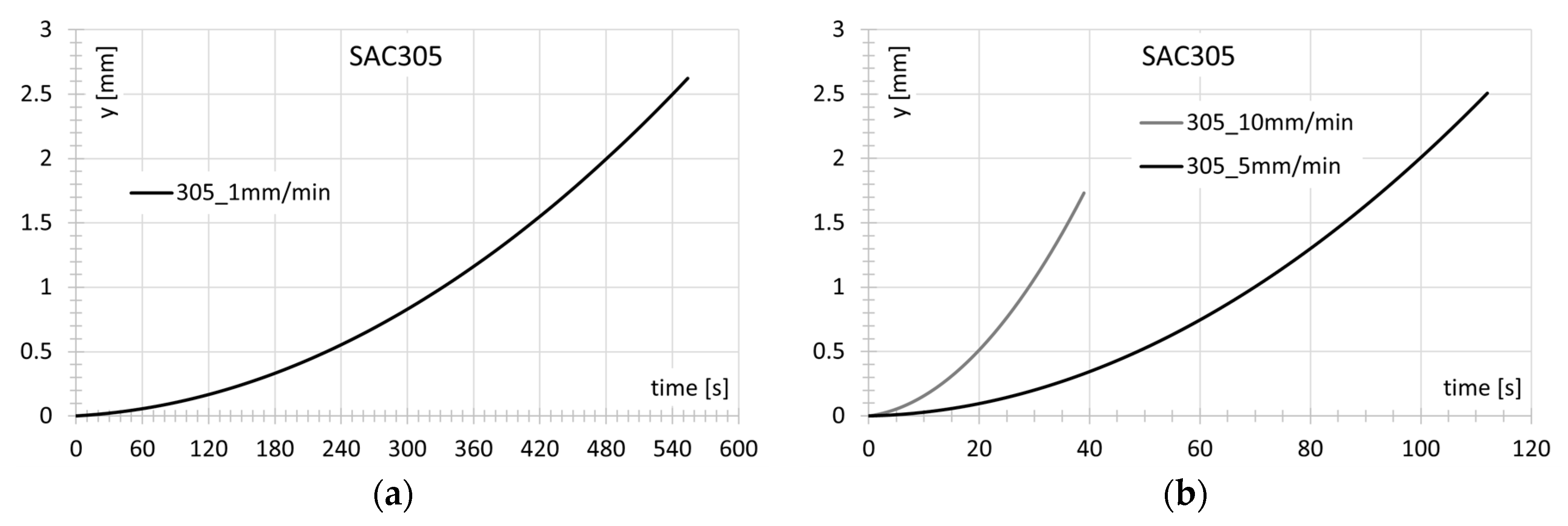
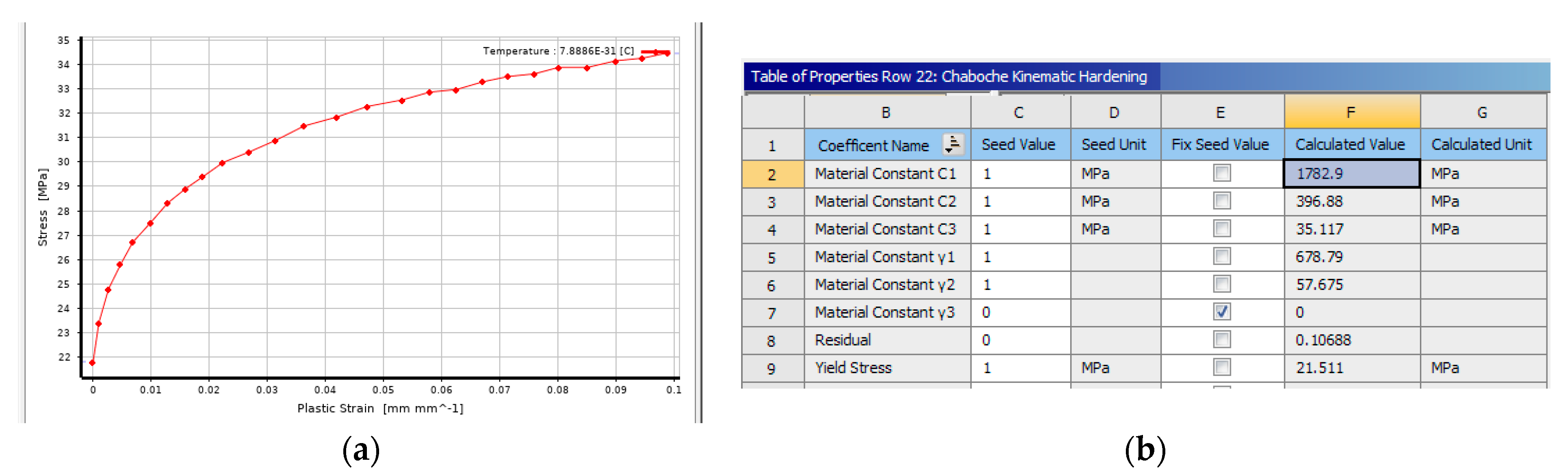
Optimisation for the Chaboche model (always ) and elastic parameter (Young modulus, yield stress): In total, seven parameters were tuned. Other parameters were fixed on their initial values. To estimate the parameters, the first tensile experiment of 1 mm/min was used.
Optimisation for the Perzyna model: two parameters were tuned. All other parameters are fixed at their initial values or values from the previous step. Two tensile experiments with different position rates (1 and 5 mm/min) were used for tuning.
Optimisation for the Chaboche model and the Perzyna model: seven parameters were tuned. All other parameters are fixed at their initial values or values from the previous step. Two tensile experiments with different strain rates (1 and 5 mm/min) were used for tuning.
Optimisation for the Norton model: two parameters were tuned. All other parameters were fixed at their values from previous steps. One creep test for the smallest cross-section (stress 28.03 MPa) was used for tuning.
Optimisation for the Norton model and the Perzyna model: in total, four parameters were tuned. All other parameters were fixed at their values from previous steps. The two creep tests for the two cross-sections (stress 28.03 and 27.22 MPa) were used for the tuning.
Optimisation for all material models: in total, nine parameters were tuned. All other parameters (E, , ) were fixed at their values from the previous steps.
Adding the last tensile test at speed 10 mm/min. Optimisation for the Chaboche model (always ) and elastic parameter (Young modulus, yield stress): in total, seven parameters were tuned. All other parameters were fixed at their values from the previous steps.
Adding the last creep test at stress 25.05 MPa. Two parameters were tuned for the Norton model. All other parameters were fixed at their values from the previous steps.
Optimisation for the Norton model and the Perzyna model: in total, four parameters were tuned. All other parameters were fixed at their values from the previous steps.
Optimisation for all material models: in total, nine parameters were tuned. All other parameters (E, , ) were fixed at their values from the previous steps.
During the identification process, the weight values for individual experiments were changed so that both types of tests (tensile tests and creep tests) had the same importance.
5.4. Settings of Identification
OptiSLang 2022 R2 software was used for the identification. The software allows one to use a lot of settings, which are keys for the identification process.
The first setting is an interval of parameter values. Each parameter has a set interval in which it can move during the optimalisation procedure. This interval is always given by a variation of from the seed value of the given parameter.
The second setting is a criterium for the termination of the optimisation cycle. We use two criteria in the paper, as follows:
Each optimalisation was run with the preset maximum number of steps. We use max. 200 steps.
During optimisation, a convergence criterion was also used. Thus, if the value of the overall objective function did not improve significantly (decrease) during 10 cycles, the optimisation was stopped.
The typical convergence curve during the minimalisation process is shown in
Figure 15. Usually, the most significant decrease was recorded during the first minimisation cycles in about 1/3, and usually there was a very gradual decrease. This course is typical of optimisation processes, so it will not be described in more detail here.
7. Discussion
In this work, an acceleration test with an hourglass specimen and DIC measurement is presented to calibrate the material model. The material model consists of three parts: Chaboche model, Perzyna model, and the Norton model. Each of the three parts captures a different component of the material behaviour, and the parameters of these models can be determined separately based on analytical relationships and selected experiments. This methodology is presented in
Section 4.3, and the parameters found are used as an initial for further calibration. In practice, such a material model is then used for FEM simulations in various commercial software. In the case of FE models, the so-called FEMU approach is then used for identification, which was used in this article to “tune” the parameter values and is briefly described in
Section 5. The solution results, see
Section 6, show that the second calibration using the FEMU approach significantly improves the quality of the solution, which is expressed by the value of the objective function (or graphs). Several problem areas were also identified during the solution. These were not analysed in more detail in the article, as the goal was to test the basic procedure.
Hourglass samples seem to generate slightly different results compared to classic samples; the problem is shown in
Section 3.2.3. Different stress states (multi-axial stress states in the hourglass sample) or slightly different manufacturing technologies can be a problem here. However, similar problems can also arise in practice.
The FEMU approach does not capture the standard physical meaning of the parameters (for example, Young’s modulus
, the value of the yield strength
) but rather the overall effect of the parameter on the given curve and approaches the material model as a black box. When using the FEMU approach, the value corresponding to the physical meaning of the parameter may deviate from this interpretation. The problem is shown in
Section 6. We can remove such parameters from FEMU identification or significantly strengthen the influence of the parameter on the resulting objective function value. However, both steps can lead to a decrease in the quality of the resulting estimate.
Another problem is determining the weights of individual experiments when calculating the value of the total objective function. Tensile tests and creep tests were used for identification. In creep tests, a large part of the error value is related to only two parameters in the Norton model. The parameter values of the Perzyna model will affect the beginning of the curve in creep tests (primary creep) and also the tensile curve at different speeds. For the Chaboche model, there will be a predominant influence in tensile tests. In this paper, creep and tensile tests were given equal weight. Through a visual comparison of the results, see
Figure 16 and
Figure 17, we came to the opinion that the creep tests show a better agreement with the experiment. There is a question as to whether the number of parameters tied to it should not be taken into account when designing weights for individual experiments.
With repetitive FEM calculations, the question arises how to reduce the required computation time? The total computational time required to tune the material model used has not been accurately measured but is estimated to take seven days. When the number of elements is reduced, significant time savings can be achieved, but the accuracy may be affected. This effect has been investigated and can be expressed using
Figure 18.
From
Figure 18a, it can be concluded that the size of the element does not have a significant effect on the precision of the tensile test results. All three curves overlap. From
Figure 18b, it can be seen that the effect of the size of the element on the accuracy of the prediction of the creep test is very small. Thus, in both cases, an element size of about 3 mm was used to minimise computational time. In
Figure 18b, the influence of time step size is investigated for 3 mm element size (1 s versus 5 s), with the conclusion that it is negligible too.
The behaviour of the tested materials is significantly affected by temperatures. The Perzyna material model was designed for one temperature and was therefore also used in this paper. Modification of Perzyna model is possible in several ways. For example, in [
42], a modification was tested that additionally adds a parameter as a function of temperature for the Anand model.
It is not possible to directly compare the obtained material model parameters with other sources as they are not yet widely available in the literature (SACX0807). In addition, the parameters depend on the temperature and the way the mechanical tests are performed. The literature [
27,
43], which is more similar to the problem presented here, can be recommended.
The inclusion of additional experiments for parameter calibration or validation of their resulting design was also considered. For the selected material model, for example, this involved the problem of ratcheting. For three material models and two types of experiments, the identification procedure consisted of 10 optimisation steps (see
Section 5.3). That is why we decided to test the basic procedure and not test temperatures or more complex states (ratcheting).


