Abstract
Recently, Asymmetric pixel–shuffle downsampling and Blind–Spot Network (AP-BSN) has made some progress in unsupervised image denoising. However, the method tends to damage the texture and edge information of the image when using pixel-shuffle downsampling (PD) to destroy pixel-related large-scale noise. To tackle this issue, we suggest a denoising method for mural images based on Cross Attention and Blind–Spot Network (CA-BSN). First, the input image is downsampled using PD, and after passing through a masked convolution module (MCM), the features are extracted respectively; then, a cross attention network (CAN) is constructed to fuse the extracted feature; finally, a feed-forward network (FFN) is introduced to strengthen the correlation between the feature, and the denoised processed image is output. The experimental results indicate that our proposed CA-BSN algorithm achieves a PSNR growth of 0.95 dB and 0.15 dB on the SIDD and DND datasets, respectively, compared to the AP-BSN algorithm. Furthermore, our method demonstrates a SSIM growth of 0.7% and 0.2% on the SIDD and DND datasets, respectively. The experiments show that our algorithm preserves the texture and edge details of the mural images better than AP-BSN, while also ensuring the denoising effect.
1. Introduction
As an important part of traditional Chinese cultural heritage and one of the oldest forms of painting, mural painting is often painted on buildings or stone walls. It reflects the political, economic, literary, artistic and technological development of the society at that time. It is valuable to historical research [1]. However, due to the natural environment and human factors, after hundreds of years, the mural paintings had problems such as mottled images, chipped walls, and alkali returning to the clay layer, which had a serious impact on the research [2,3,4]. The processing of mural images has been slow because of the massive engineering, restricted technology, rare talent, and limited resources. It can take a few months to a year or two to process a mural image [5,6]. Mural images are exposed to air for a long time, and there are typical problems such as fuzzy edges, unclear outlines, noise or color spots are obvious; that is why it is necessary to deal with the problem of noise pollution in the processing of mural images.
Images that are affected by equipment or the external environment, or that have color spots and noise, are classified as noisy images. Image denoising refers to recovering a clean or noise-free image from a noisy image. Image denoising is fundamental research in low-level vision [7]. Noise can greatly degrade the image quality, and the denoising effect directly affects other subsequent processing steps [8]. The use of an image denoising method in the digital processing of mural images can eliminate any extraneous noise and spots present in mural images. Additionally, this technique may provide a groundwork for subsequent image processing operations.
The traditional image denoising methods mainly include mean filtering [9], median filtering [10] and wavelet transform [11], which are insufficient because they have poor robustness in the real world and cannot accurately and efficiently remove noise from images [12]. With the development of deep learning, image denoising algorithms based on deep learning have been widely used due to their efficient and convenient characteristics and have become an effective solution to deal with image denoising.
Noise is not isolated in pixels in real scenes. There is spatial correlation between most pixel points. In a recent study, AP-BSN [13] takes into account the connection between noisy pixels, and the study proposes to combine PD and BSN to match noisy images in real scenes more closely. AP-BSN first uses downsampling to decompose the noisy image into multiple sub-images, destroys the spatial correlation of noise, and then utilizes the correlation of the surrounding pixels to map out the original pixels under the noisy pixels. However, the presence of larger-scale noise means that if we do not consider the texture information but only focus on how to destroy the spatial noise, drastically destroying the spatial correlation of noise at the same time will also cause a certain degree of damage to the texture information of image, which will add a certain degree of difficulty to the process of the mural images.
To this end, we propose a feature extraction network (FEN) to extract global and local feature of the mural images, respectively, and we use two cross–attention blocks for fusion and information interaction between the features, focusing on retaining texture information while denoising. We evaluate this on the mainstream noisy image datasets Smartphone Image Denoising Dataset (SIDD) [14], Darmstadt Noise Dataset (DND) [15], and our homemade mural noise image dataset. In order to show the experimental effect better, we design comparative experiments. Our method shows better results compared with several representative image denoising methods, not only performing effective denoising, but also retaining more edge and texture information. We summarize our contributions as follows:
- (1)
- In order to further extract the feature information utilizing the image denoising process, we design the densely dilated residual block (DDR) and non-local attention mechanism (NLA) to extract the local and global feature information, respectively. The denoising performance is enhanced while preserving the texture and structure information of the image as much as possible.
- (2)
- We construct local and global cross attention block (LGCA) and feature fusion cross attention block (FFCA) for fusing the local and global information of feature extraction and the feature before and after feature processing, respectively. In this way, the interaction between feature information is enhanced.
- (3)
- Our method is evaluated on two mainstream image denoising datasets and a homemade mural images dataset, and our method achieves commendable performance.
2. Related Works
Existing image denoising methods can be categorized into two groups based on the availability of clean images as data labels. They are supervised learning and unsupervised learning. Supervised denoising requires a large number of noisy-clean image pairs, where noisy images refer to images containing noise and clean images refer to images without noise, these image pairs are often difficult to obtain in real scenes and require a lot of human and material resources. A common approach is to add simulated real-world noise (e.g., Additive White Gaussian White Noise, AWGN) to a clean image as a pairing of a noise image and a clean image [12,16,17,18]. However, there is still a gap between the real-world and synthesized noise. The model trained using the synthesized noise is less capable of performing in the real scenes. In some cases, it may also be difficult to obtain clean images. In such cases, unsupervised denoising methods show a unique advantage because no clean image is required as data labels.
2.1. Supervised Image Denoising
Zhang et al. [16] first applied deep learning to the image denoising task in DnCNN, proposing a supervised method for processing noise using noisy-clean pairs. The method uses Convolutional Neural Networks (CNN) to process noisy images, trains the model by manually adding AWGN to the clean noise, and uses residual learning to improve the denoising performance of the network model. In the subsequent development, Zhang et al. introduced FFDNet [17] and CBDNet [18] algorithms to adapt the network model to real scene noise while balancing denoising and detail preservation. The shortcoming is that CBDNet is a two-stage denoising network, which is not efficient and flexible enough. Based on this, Anwar et al. [19] proposed RIDNet network structure, a one-stage algorithm that is more practical for denoising, using a self-attention mechanism to adjust the feature at the channel level, which improves the denoising effect of the model. Ren et al. [20] proposed a novel deep network for image denoising. Unlike most existing deep network-based denoising methods, Ren incorporated Adaptive Consistency Prior (ACP) into the optimization problem and used an unfolding strategy to inform the design of deep the network during the optimization process. All the above methods have some logic to follow, but one of the main problems faced by image denoising is the lack of noisy–clean pairs in real scenes. The collection cost of clean images is high. It is more challenging to adapt the model to different application scenarios. Therefore, it has significant value to investigate unsupervised learning and mine the data for potential properties.
2.2. Unsupervised Image Denoising
Lehtinen et al. [21] proposed Noise2Noise, where the network can use noisy images to learn to transform noisy images into clean images. They held the belief that since the input and output noise is random, going to force the learning of the relationship between the two will have two results using CNN. With fewer training samples, the CNN learns the transition relationship between the two noise patterns. When the number of samples is large enough, since the noise is randomly unpredictable and stands to minimize the loss, the convolution can learn the clean image itself. This method has the disadvantage of requiring various noisy image pairs. Noise2Noise is only suitable for a part of the cases. Considering this, Alexander et al. [22] proposed Noise2Void, which uses BSN to denoise directly on a single image. The BSN assumes that the pixels of a real image are conditionally correlated, while the noise pixels are independent of each other and are not correlated with each other. A neural network uses this implicit information about a contaminated pixel point to infer the true value of the contaminated portion by looking at the pixel points around it. However, real noise does not necessarily satisfy the assumption that pixels are independent and have zero mean, so this method is less effective in dealing with structured noise. Laine19 [23] and Xu et al. [24] further used BSN to deal with noise in images; the shortcoming is that the convolution’s structure restricts the network model from utilizing the remote information to take full advantage of the global feature. Hong et al. [25] proposed using a conditional adversarial network for adversarial training between generators and discriminators. Still, this method is demanding on the training data, and the model is prone to overfitting. Denoising may not be effective if multiple noise types are present. In order to ease the loss of pixel information caused by BSN denoising, Wang et al. [26] added a branch to Noise2Void and improved the denoising performance of BSN by introducing non-blind point denoising. However, the method works under the assumption of noise pixel independence and is less effective in removing noise with spatial correlation. Neshatavar et al. [27] proposed CVF-SID to separate the noise component from the clean image; it assumes that the noise space is uncorrelated, which does not match the true noise distribution. Lee et al. [13] used Asymmetric PD (AP) for real-world noise to break the spatial correlation of noise, which destroys the structural noise by separating neighboring pixels into different small-size maps. However, the choice to use a larger PD step size to destroy the larger scale noise can also have some impact on the image details, destroying the texture’s coherence [28]. Therefore, maintaining a balance between image denoising and preserving high-frequency information such as textures and edges is an urgent problem.
Denoising is an indispensable part of a mural images’ digitization process. It has better adaptability to the use of unsupervised denoising methods for model training when not having clean mural images as data labels. Therefore, we use a feature extraction network (FEN) to extract global and local features, construct two cross-attention blocks to fuse the information of each stage, and enhance the nonlinear expression ability of the network through the processing of a feed-forward network (FFN). While ensuring the image denoising effect, high-frequency information such as texture is retained as much as possible to reduce the loss of information in the detailed part of the image.
3. Methods
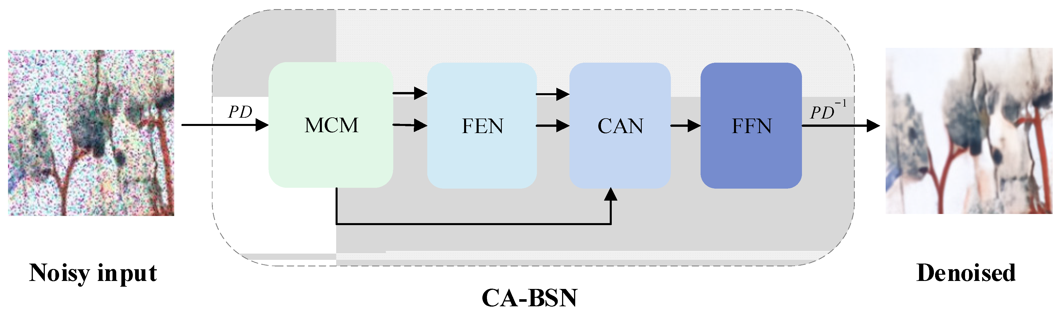
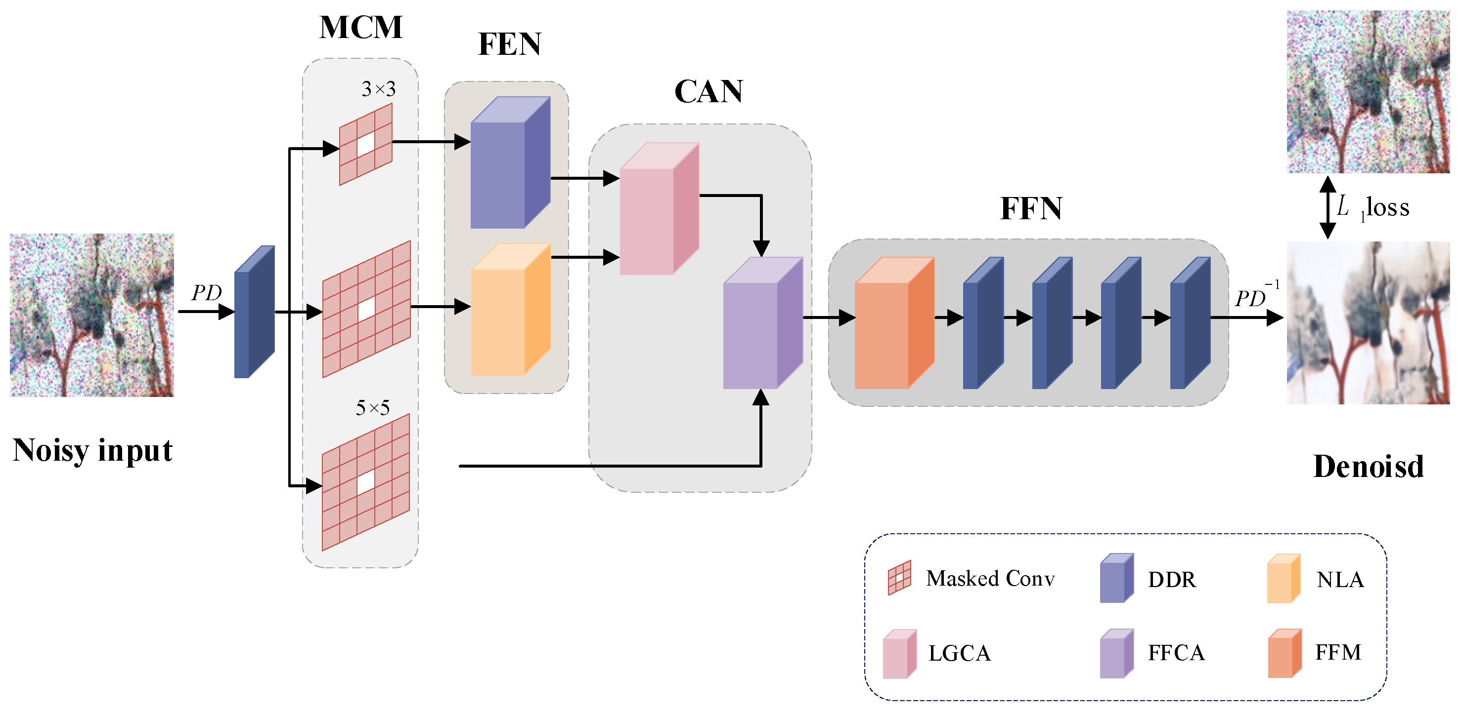
In response to the loss of other high-frequency information due to the pursuit of the denoising effect during mural restoration, we propose CA-BSN. We first illustrate the overall algorithm in Figure 1.

Figure 1.
The flow of the algorithm.
First, we use PD to sample the mural image containing large-scale noise into multiple small-size images, and we input into masked convolution module (MCM) and feature extraction network (FEN), respectively, to extract feature information. Then, the cross attention network (CAN) is constructed to fuse the feature information, which includes two independent cross-attention blocks, and feature fusion is performed separately for different parts. Finally, the nonlinear expression ability of the model is improved by a feed-forward network (FFN), and the denoised image is output.
3.1. Feature Extraction Network Construction
The masked convolution module (MCM) contains three branches; the small image obtained after PD processing goes through the center mask convolution with a convolution kernel size of 3 × 3 and 5 × 5 in two branches to obtain the local input feature and global input feature, respectively, and through the center mask convolution layer with a convolution kernel size of 5 × 5 in the last branch to obtain the previous feature.
Existing blind spot denoising algorithms usually overlap using multiple dilated convolutions containing skip connection to realize the reuse of feature information. However, capturing the contextual information only by increasing the network sensing field is prone to a loss of information, making some pixels not involved in the convolution operation from beginning to end and underutilizing the feature information. In contrast to CNN, the self-attention mechanism in Transformer [29,30] allows the model to acquire information from arbitrary locations. This feature enables Transformer to better capture feature dependencies over long distances and ensure global feature extraction, making up for the limitations of the CNN in the global feature extraction process. The attention mechanism has a high computational complexity, and in some cases, it is more efficient to use convolution. Therefore, to fully extract and utilize the feature information in the image denoising process, we design the feature extraction network to include two parallel branches: a densely dilated residual block (DDR) for extracting local feature information, and a non-local attention mechanism (NLA) for extracting global feature information. In this way, the advantages of both mechanisms can be fully exploited to improve the performance of the model.
3.1.1. Densely Dilated Residual Block Construction
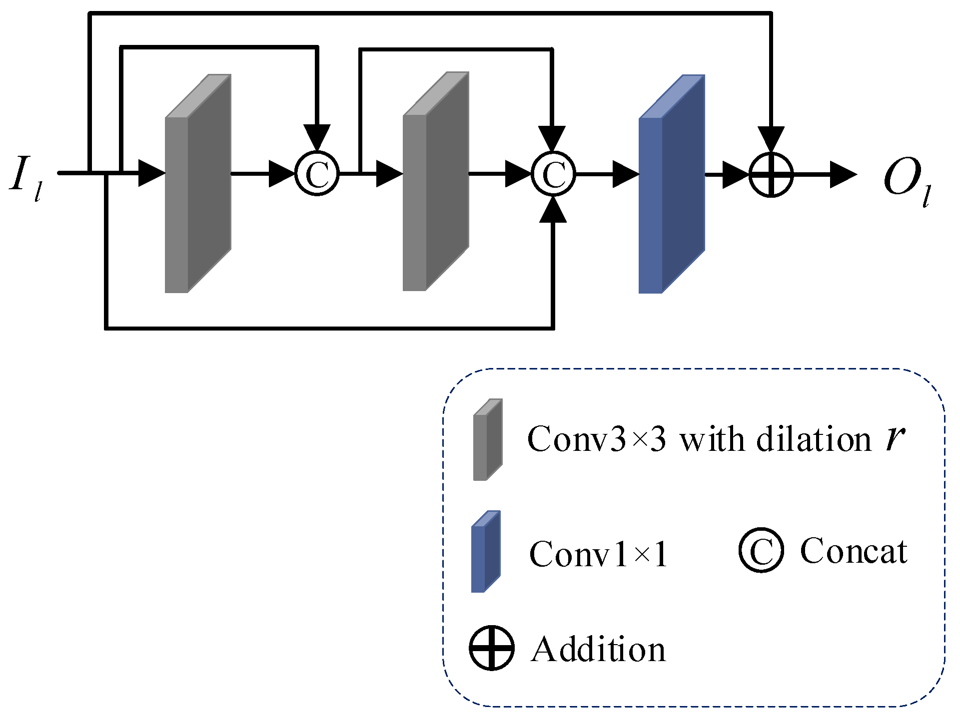
The dilated convolution extends the field of view of the convolution filter over the feature map by adding dilation between neighboring filter pixels during convolution, using the expanded sense field to allow the network to extract more contextual information and reduce computational cost. To fully utilize the information extracted from the convolution of each layer, we propose a densely dilated residual block (DDR), which combines densely connected residual blocks and dilated convolution under the guarantee of the denoising performance of the mural image, which enhances the information exchange between the layers and obtains richer feature information while reducing the number of references. The structure of densely dilated residual block (DDR) is shown in Figure 2.
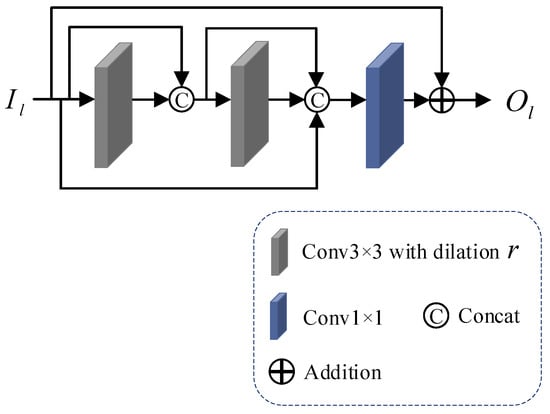
Figure 2.
The structure of densely dilated residual block.
First, the local input feature is sequentially passed through two dilated convolution layers, and , with a convolution kernel size of 3 × 3, where denotes the dilated rate, the convolution kernel 3 × 3 in size is the most commonly used filter size in image denoising, and the feature obtained from each pass through the dilated convolution layer and the feature of the previous layer are channel-summing using . After the two-layer feature extraction process, an overall channel-summing is performed to obtain the feature information . The complete calculation process is shown in Equation (1):
Then, feature fusion and channel processing are performed using 1 × 1 convolution on .
Finally, the skip connection is used to transfer the shallow feature information to the deeper convolutional layer to output the local feature . The computational procedure is shown in Equation (2):
After the above steps of feature extraction and feature fusion, we obtain the locally extracted information of the image, ensuring the denoising performance of the mural image.
3.1.2. Non-Local Attention Mechanism Introduction
In order to enhance the model to extract and utilize the global information of the image and retain the texture information of the image, we introduce a non-local attention mechanism (NLA) to adjust the processing based on the dynamic weights of the input image feature. The structure of the non-local attention mechanism (NLA) is shown below in Figure 3.
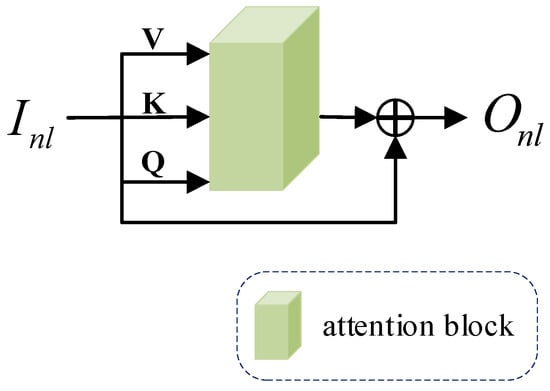
Figure 3.
The structure of non-local attention mechanism.
Our non-local attention mechanism (NLA) is divided into two main steps. First, calculate the attention block; then, output the global feature. The specific steps are as follows.
Step 1. Calculate the attention block.
The attention block is a structure of interactive operations through Value (V), Key (K), Query (Q) matrices, as shown in Figure 4 below.
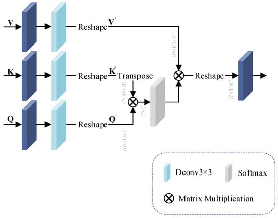
Figure 4.
The structure of attention block.
In neural networks, deep convolution can use fewer parameters than normal convolution by performing a separate convolution operation for each channel. Therefore, after changing the number of feature channels in the 1 × 1 convolution, we use deep convolution instead of the previously used convolution for arithmetic processing.
In attention block, first, for the input , and matrices, the feature are extracted using 1 × 1 convolution and 3 × 3 deep convolution , respectively, and the , and dimensions are changed to using the Reshape operation . The process is computed as shown in Equations (3)–(5):
Then, the matrix after transposition of is multiplied with the matrix , and the mapping operation is performed using the function to obtain the correlation weight between the two input matrices. This step of the computation is shown in Equation (6):
Finally, the weight matrix is calculated using weight and . The calculation process is shown in Equation (7):
Step 2. Export global feature.
The input feature is . Different components , and are input into the attention block to get the weight matrix to establish the correlation between the global features. We use the skip connection to ensure the learning performance of the network model to output global feature . The calculation process is shown in Equation (8):
By using non-local attention mechanism (NLA) based on the self-attention mechanism, the extraction of global feature information can be enhanced to make up for the shortcomings of densely dilated residual block (DDR) in global feature extraction and retain as much as possible the texture and edge information of the mural image that is easily lost in the process of local feature extraction.
3.2. Cross Attention Network Construction
We construct a cross attention network (CAN), which contains LGCA and FFCA to fuse feature and enhance the interaction between feature information. LGCA fuses local and global features, and FFCA fuses local–global feature outputs by LGCA and the previous feature.
3.2.1. Local and Global Cross Attention Block Construction
The constructed cross attention block can effectively handle the relationship between two distinct features and enhances information extraction by integrating data from multiple sources, surpassing the general self-attention mechanism in performance. Our LGCA primarily consists of layer normalization (LN) and attention block, as illustrated in Figure 5 below.
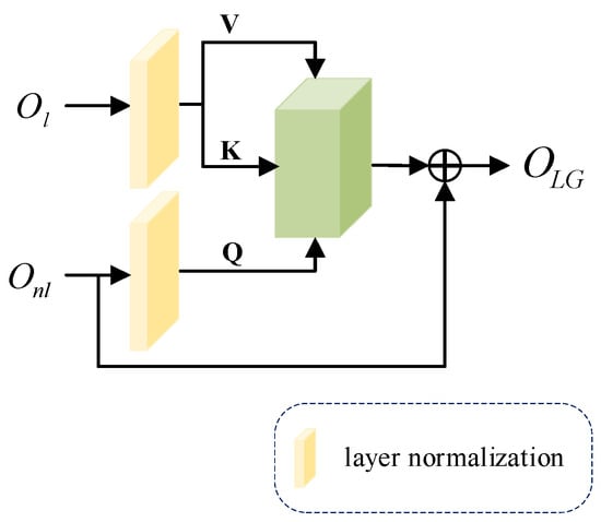
Figure 5.
The structure of local and global cross attention block.
Specifically, we first use the features and obtained from densely dilated residual block (DDR) and non-local attention mechanism (NLA) as different inputs, which are processed by the normalization layer . The is mapped into matrices and , and is mapped into matrix .
The , and obtained from different feature mappings are input into the attention block, the weight matrix is calculated, and a layer of skip connections is added to output the feature matrix obtained from cross attention. The calculation process is shown in Equation (9):
We can enhance the interaction of the mural images’ local and global information and better fuse important information by dealing with the relationship between different features.
3.2.2. Feature Fusion Cross Attention Block Construction
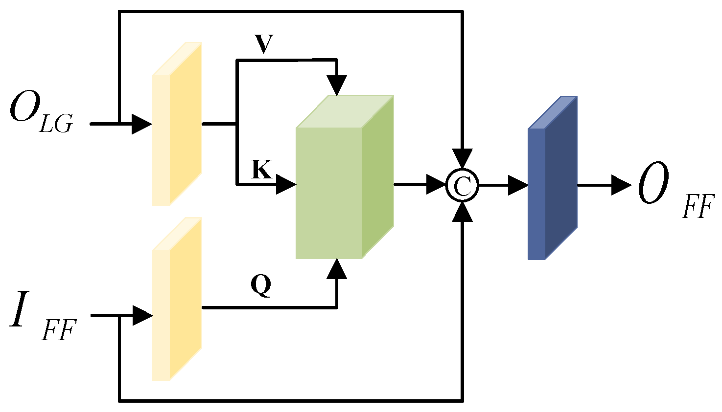
We construct an FFCA to fuse the feature information before and after feature extraction fully. Like LGCA, the FFCA extracts feature information based on attention blocks, and strengthen the global relevance of previous and later features by enhancing the information interaction previous and later feature processing. The specific structure is shown in Figure 6.
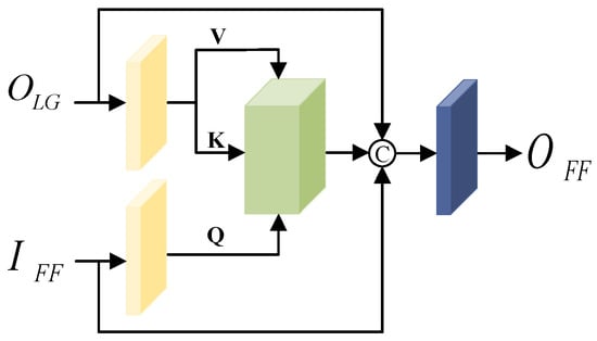
Figure 6.
The structure of feature fusion cross attention block.
First, the feature output from LGCA and the previous feature are used as inputs to cross attention block, and the feature matrices , and are obtained after the normalization layer.
Then, the , and are fed into attention block, the features obtained from the cross attention block are fused with the input features using channel summation, and the output features are obtained by processing the number of channels through a 1 × 1 convolutional layer. The computational procedure is shown in Equation (10):
Fusing feature information from different paths using two different cross attention blocks enhances the information exchange between features and can fully utilize the local and global information in the denoising process.
3.3. Feed Forward Network Introduction
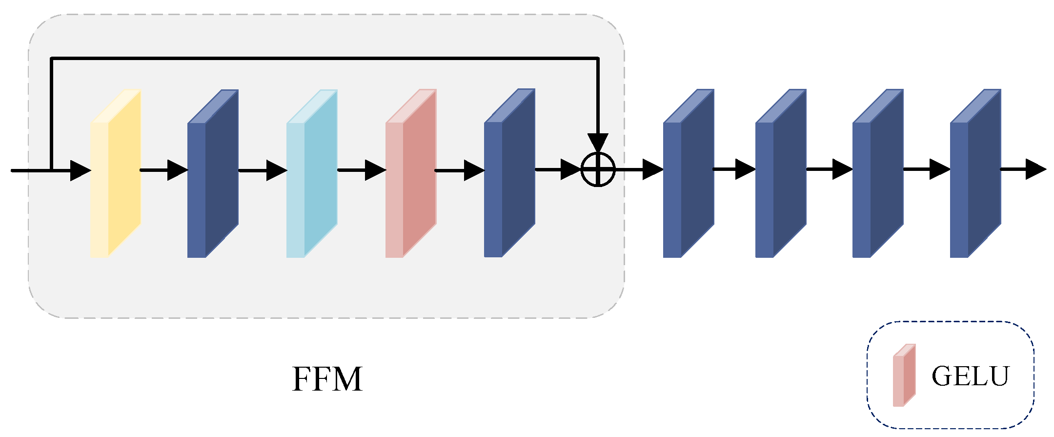
The feed-forward network (FFN) consists of a feed-forward module (FFM) and four 1 × 1 convolutional layers; the structure is shown in Figure 7.

Figure 7.
The structure of feed-forward network.
We use the feed-forward module (FFM) to enhance the nonlinear expression of FFCA. The computational procedure is shown in Equation (11):
where belongs to the class of activation functions, and denotes the result obtained by after feed-forward module (FFM) processing. Finally, the output after denoising is calculated by superimposing multiple 1 × 1 convolutions.
After the above steps of the cross fusion of different path information, the high-frequency information is retained as much as possible while guaranteeing the denoising effect, which enables our method to achieve better performance results in mural image denoising. The overall CA-BSN architecture is shown in Figure 8.
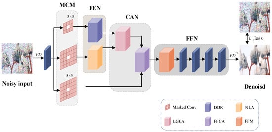
Figure 8.
The architecture of mural image denoising method based on Cross Attention and Blind-Spot Network.
The original noise-containing mural image is sampled into multiple small images after PD, and the sampled image is passed through a 1 × 1 convolutional layer used for linear transformations. First, the feature information is passed through a masked convolution module (MCM) containing three parallel center mask convolutions, and the local input features and global input features obtained after mask convolution are processed using the densely dilated residual block (DDR) and non-local attention mechanism (NLA) in feature extraction network (FEN), respectively. Then, the local and global features obtained after feature extraction are fused by LGCA, and the feature output from LGCA and the previous feature obtained after the 5 × 5 mask convolution are fused by FFCA. Finally, the feature information is passed through a feed-forward network (FFN) consisting of a feed-forward module (FFM) and multiple 1 × 1 convolutions, which is used to upsample multiple processed small-size maps into a single denoised mural image.
We train the CA-BSN using the loss . The computational procedure is shown in Equations (12) and (13):
We first use to break the spatial connection between the noises of neighboring pixels, decompose the noisy image into smaller images, then use the whole network for denoising, and finally combine the outputs through to get the denoising result with the same size as the original image.
4. Experiments
In this section, we first describe the datasets and evaluation metrics during the experiments, then describe the implementation details, followed by a comparative study with previous related denoising algorithms to compare the denoising effect of our algorithmic model, and finally design an ablation study to validate the impact of each module in CA-BSN on the overall performance.
4.1. Dataset and Evaluation Metric
Our approach is evaluated on two real-world datasets, SIDD and DND, which are mainstreams in image denoising. The SIDD is a set of about 30,000 noise-containing images obtained from five representative smartphone cameras in ten scenes under different lighting conditions, along with the corresponding clean images. We selected sRGB images from SIDD-Medium with 320 noisy-clean pairs for model training. We use sRGB images from the SIDD validation set and benchmarks with 40 images per category, each of which can be cropped to 1280 image blocks of 256 × 256 size, for validation and evaluation. The DND consists of 50 noisy images, including indoor and outdoor scenes, there are no clear images, and the denoising results can only be obtained by an online system. Since our method does not need to consider clean images, the DND can be used directly as a training and test set.
Our method belongs to a kind of unsupervised denoising, self-supervised denoising. In order to better adapt the model to mural images and demonstrate the denoising effect of CA-BSN on mural images, we construct a small mural dataset. We retain the mural dataset used in the lab in the past and obtained some electronic images by collecting classic books and official museum displays, and extended the dataset by cropping, rotating, and flipping, which are the ground-truth data.
In order to obtain random and natural noisy images, we analyze the noise characteristics of the images, which are mainly characterized by irregular distribution and size, spatial correlation of noise, and mixing of multiple types of noise. Therefore, we chose to add Gaussian noise, Poisson noise and Perlin noise. The specific formulas are as follows:
where denotes the number of times the noise was added, is an intermediate variable, and is the data obtained after has been added by the Gaussian, Poisson, and Perlin noise. Item is the random mixing ratio of Gaussian and Poisson noise ranging from 0.3 to 0.7. denotes the Gaussian noise with mean and standard deviation . The mean value ranges from −1.0 to 1.0 and standard deviation from 9 to 25. denotes Poisson noise with intensity and a random range of intensity from 8 to 12. denotes the equation for two-dimensional Perlin noise distribution, where the scale has a random range of 8 to 12, octaves of 4 to 8, persistence between 0.3 and 0.7, and lacunarity of 1.5 to 3.0. By superimposing the noise on each image several times, we obtain a batch of mural noise images that satisfy the image noise properties but are still natural.
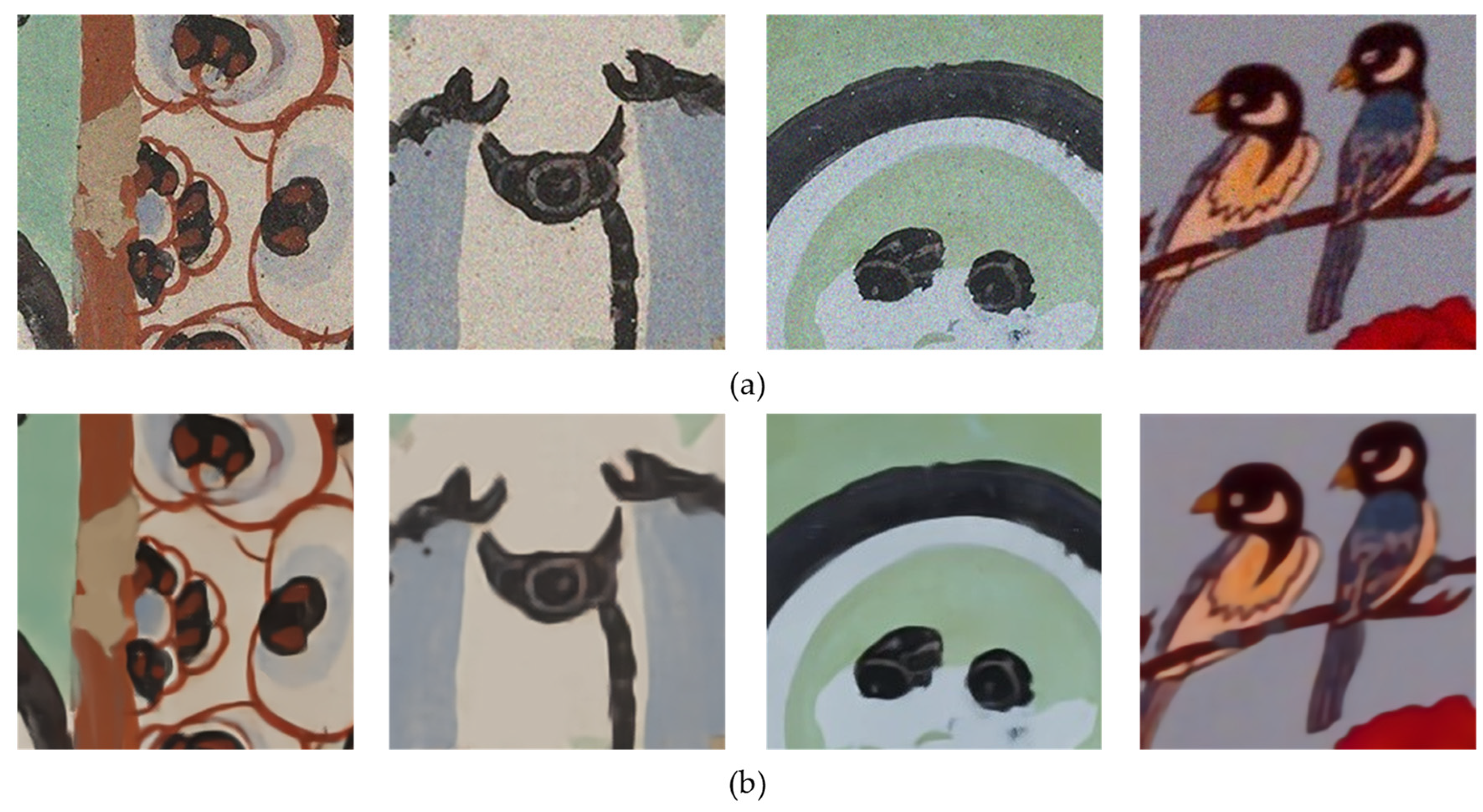
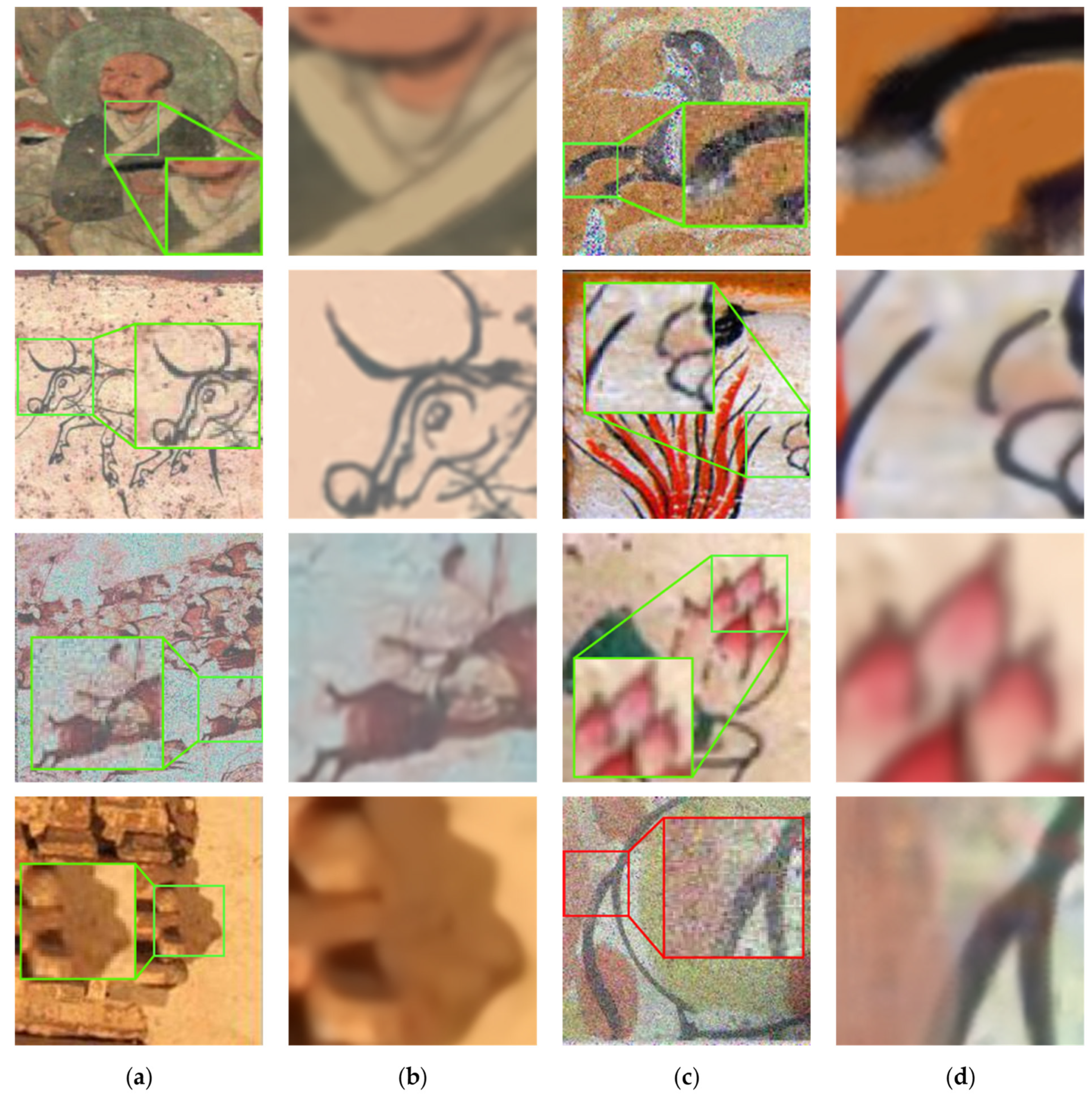
Since our method does not use ground truth data, we directly use the noisy mural dataset for training and testing. The ground truth data are used to compare metrics. The mural images in our paper are sRGB data containing 15,000 patches of size 224 × 224, mainly Buddhist culture and ancient scenes. Partial samples of the dataset are shown in Figure 9.
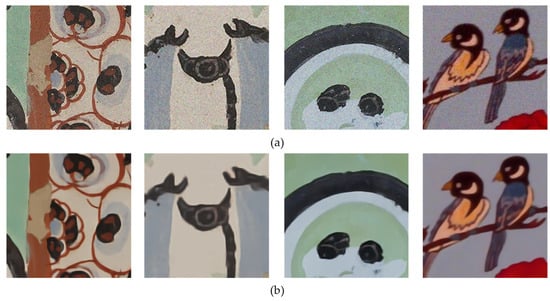
Figure 9.
Partial mural dataset presentation. (a) are examples from noisy images, and (b) are from ground truth data.
In order to verify the denoising effect of the model, we use the Peak Signal-to-Noise Ratio (PSNR) and the Structural Similarity Index Measure (SSIM) as objective evaluation metrics. PSNR is used to measure the quality of the image, and SSIM measures the similarity of the two images. Higher PSNR and SSIM values indicate improved output image quality.
4.2. Implementation Details
The computer hardware environment used during the overall experiment is the Intel(R) Xeon(R) Silver 4110 CPU @ 2.10 GHz, 64 GB of RAM, and NVIDIA Quadro RTX 6000 graphics card; the software environment is the Windows 10 operating system; and the runtime environments are Python3.10, PyTorch2.0 and Pycharm2022.3.3. The experiment uses the Adam optimizer with the initial learning rate set to , and the batch size is set to 32. The total number of rounds of model training is 30, and the learning rate is multiplied by 0.1 at round 20. In this paper, the asymmetric pixel–shuffle downsampling proposed by AP-BSN is followed, and the PD stride is set to 5 in the training phase and 2 in the testing phase.
4.3. Comparison Experiment
In order to verify the feasibility and effectiveness of our proposed CA-BSN, we designed comparison experiments of image denoising. Table 1 demonstrates the comparison results of several methods on the SIDD and DND datasets for the objective evaluation index parameters. Figure 10 shows the visualization results of some of the methods in Table 1 on the DND and SIDD.

Table 1.
Quantitative comparison of different denoising models on SIDD and DND. We use “AP-BSN” in the paper to represent “” in paper [13]. Therefore, the “AP-BSN” here is consistent with the value of “” in the paper. By default, we get the official evaluation results from SIDD and DND benchmark websites. R indicates that the result is reported by R2R [31]. † indicates that we have retrained the model in the same way as our implementation details. The highest value is highlighted in bold for each type of denoising model.
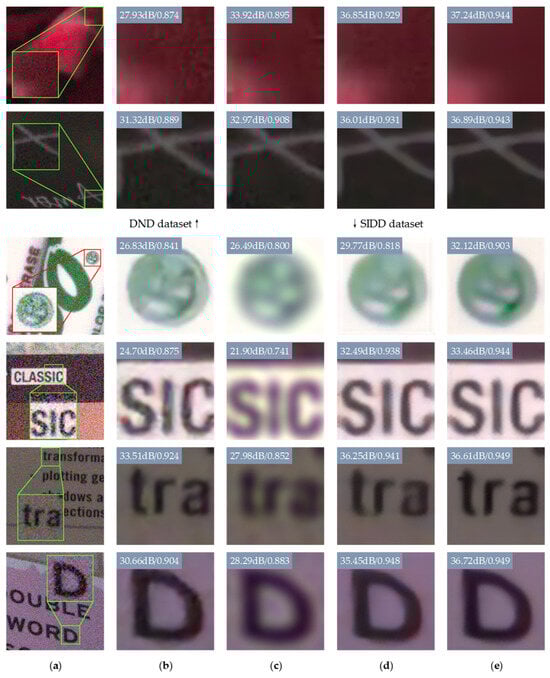
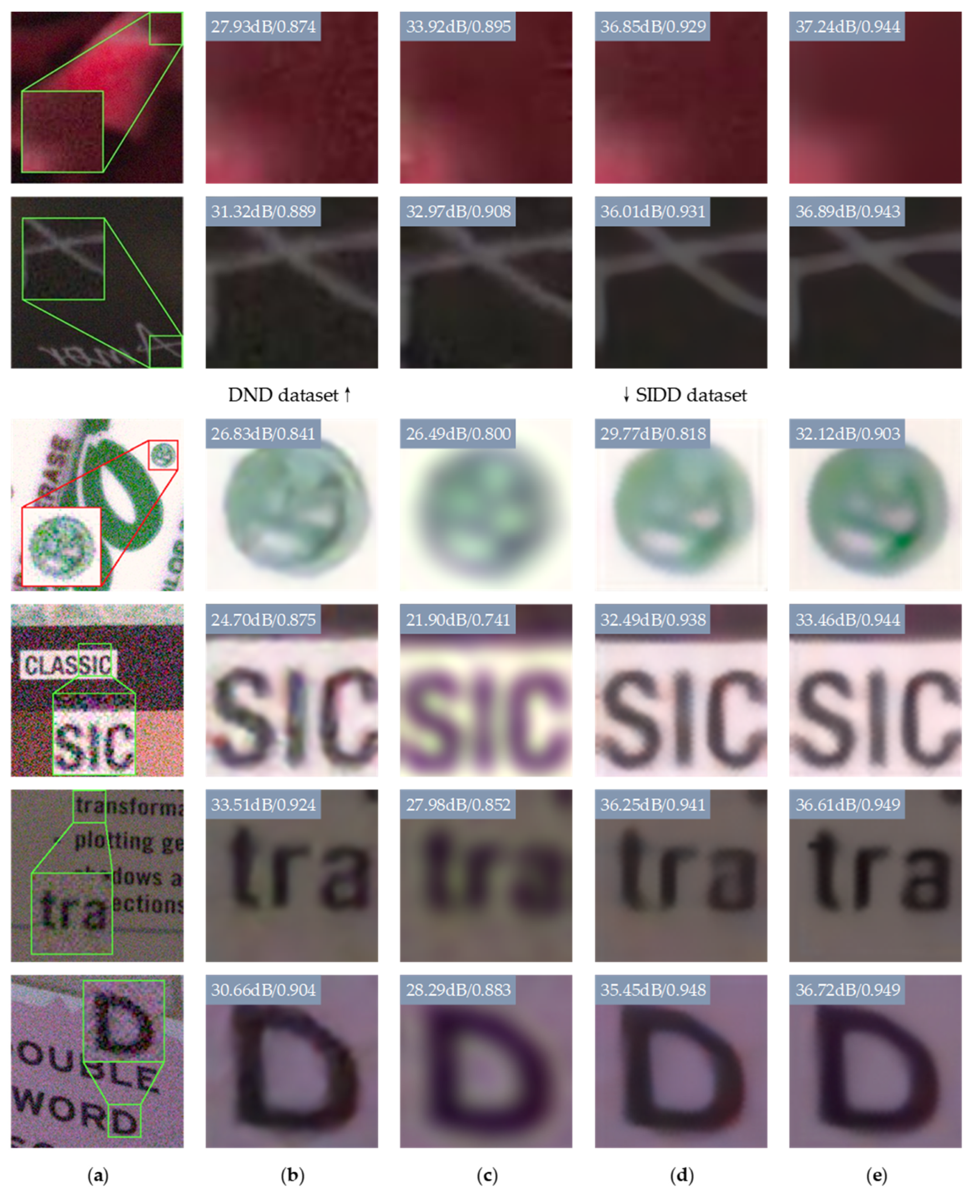
Figure 10.
Comparison of visual quality of DND and SIDD images. The upper two rows are examples from the DND dataset, and the lower four rows are from the SIDD dataset. (a) Noisy (b) CBDNet (c) CVF-SID (d) AP-BSN (e) Ours. Best viewed zoomed in. For quantitative comparison, we mark per-sample PSNR/SSIM w.r.t. the ground-truth image at the upper left of each patch.
The methods we compared include non-learning based, supervised denoising, and unsupervised methods. As can be seen from Table 1, RIDNet has achieved impressive performance in denoising. However, our analysis focuses on unsupervised denoising, and although RIDNet’s performance is noteworthy, it is not suitable for the denoising of mural images due to the difference in categories and the limitation of the application scenarios, which are worse in the application of mural images. Our method outperforms previous unsupervised representative methods in both SIDD and DND, demonstrating excellent denoising performance. Specifically, our proposed CA-BSN improves the PSNR by 0.95 and 0.15 on the two datasets, and the SSIM also grows by 0.7% and 0.2%, respectively, compared to the AP-BSN algorithm.
In Figure 10, we show two images from the DND and four images from the SIDD processed by different denoising models. Figure 10a shows the original noisy image, which we zoomed in locally for a more visual comparison with the other methods. Because of our limited time and equipment resources, we choose CBDNet, which saves more training time and model computation compared to RIDNet, as a comparative method to show the test effect. The supervised learning-based method CBDNet cannot clearly discriminate the image’s high frequency details due to its model’s characteristics, which leads to the situation that the edge information is prone to be deficient, and the model’s generalization ability in different scenes is weak. In the unsupervised denoising model, for the direct observation method using a single noisy image, CVF-SID does not take into account the spatial correlation of the real noise, only considers the separation of the noise from the clean image, and the real noise cannot be removed entirely. Figure 10c shows that this approach can blur image edges. The AP-BSN algorithm simply loses some pixel information using dilated convolution and destroys the texture information of the image using PD with a large step size, as seen in Figure 10d. AP-BSN performs poorly in the detailed parts such as edges. Our proposed CA-BSN algorithm designs spatial correlation and remote dependency into the network, preserving the detailed information as much as possible. According to Figure 10e we can see that compared with other algorithms, the edges of the images processed by our CA-BSN are clearer and show better denoising effect.
In order to test the denoising effect of our method on the mural dataset, we compare it with the current more popular unsupervised denoising methods, and the results on the evaluation metrics are shown in Table 2.
Table 2.
Quantitative comparison of different denoising models on mural images dataset. The highest value is highlighted in bold for denoising models.
In order to verify the specific performance effect of our proposed method in the process of mural image denoising, we select several images from the mural dataset for effect demonstration and visually compare the different unsupervised methods in Table 2. The results are shown in Figure 11.

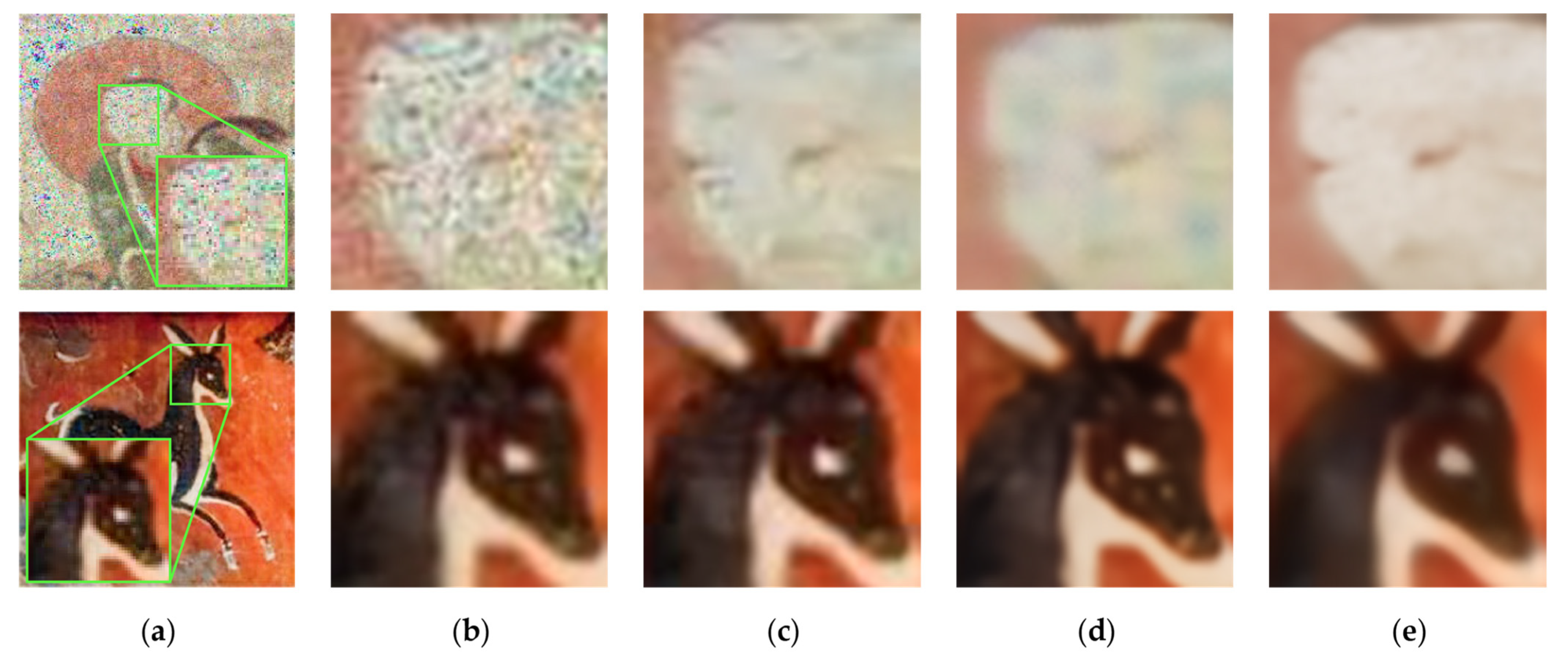
Figure 11.
Comparison of visual quality of mural images. (a) Noisy (b) Noise2Void (c) CVF-SID (d) AP-BSN (e) Ours. Best viewed zoomed in.
We have chosen three unsupervised methods, Noise2Void, CVF-SID and AP-BSN, to compare with our method. As can be seen from the figure, compared with the three methods, our denoising method has better performance on the mural image, the color spots in the image are removed more completely, and the texture information, which is not very distinguishable from the surrounding noise, is also well preserved, reducing the loss, and the texture part is shown more clearly.
Figure 12 displays the denoising effect of CA-BSN on mural images.

Figure 12.
Mural images denoising effect display. (a) Noisy (b) Ours (c) Noisy (d) Ours. Best viewed zoomed in.
4.4. Ablation Study
In order to validate the impact that each module brings to the denoising of mural images in our method, we designed ablation studies based on two evaluation metrics, PSNR and SSIM, on the mainstream SIDD.
We verify the effect of different convolution kernel sizes and masked sizes of masked convolution layers in the masked convolution module (MCM) on model training. The role of the convolution kernel in the masked convolution layer is to extract features, and the mask is mainly used for blind spot mapping in the subsequent network, demonstrating the impact on model performance and the number of parameters through changes in convolution kernel and masked size. The specific details are shown in Table 3.
Table 3.
Ablation study with different convolution kernels and masked sizes. The highest value is highlighted in bold for denoising models.
“Masked Conv1” denotes the masked convolution used to extract local features, “Masked Conv2” denotes the masked convolution used to extract global features, and “Masked Conv3” denotes the masked convolution used to extract previous features. The size of the convolution kernel affects the extraction of features, the small convolution kernel is suitable for extracting the detailed information of the image, and the large convolution kernel is suitable for extracting the overall information of the image. The larger the size of the convolution kernel, the higher the number of parameters in the computational equation. The size of the mask affects some information in the pixels of the image; when a larger mask is used, the texture information of the image may be lost due to occlusion. The larger the masked size, the less data are involved in the computation.
In order to verify the superiority of our designed feature extraction network (FEN) and cross attention network (CAN), we designed an ablation study using the substitution method as shown in Table 4.
Table 4.
Ablation study with feature extraction and fusion. The highest value is highlighted in bold for denoising models.
Case (e) is our method, Case (a) is to replace both parts of the feature extraction with global feature extraction using attention mechanism, Case (b) is to replace both parts of the feature extraction with local feature extraction using convolution operation, and Case (c) and Case (d) are to replace the cross-feature fusion part with the common “concat” in turn. Table 4 shows the model performance and the amount of computation for different settings. Experiments show that the feature extraction combining the convolution and attention mechanisms is more effective for model training.
We designed an ablation study to verify the effect of different convolutional layers for the number of 1 × 1 convolutional layers for multiple after feed-forward modules (FFMs) in the feed-forward network (FFN). The details are shown in Table 5.
Table 5.
Ablation study with different number of convolutional layers. The highest value is highlighted in bold for denoising models.
The “1 × Conv” indicates that only one 1 × 1 convolutional layer is used in the final feature extraction for channel processing and information interaction, and according to the parameters in the table, we can see that the use of four 1 × 1 convolutional layers is better, and the method we use has better performance.
To verify the effect of using different modules on the image denoising performance, we designed an ablation study with different modules, as shown in Table 6.
Table 6.
Ablation study using different modules. The highest value is highlighted in bold for denoising models.
The “×” indicates that the module was not used in that experiment, and “√” indicates that the module was added. Case (a) is our baseline; here, we only consider whether the module is used or not, without considering other factors (e.g., parameter settings). Since the benchmarks only consider local and global performance, they are not highly utilized for features before and after image processing. When we connect the FFN and FFCA, i.e., Cases (b) and (c), the model achieves an increase of 0.26 dB and 4.17 dB, respectively. Based on the results of the parameters of PSNR and SSIM in the table, it can be seen that Case (d) using LGCA, FECA and the feed-forward network (FFN) have better performance.
5. Conclusions
In this paper, we propose CA-BSN for denoising mural images, aiming to denoise the image while preserving the texture details of the image. First, we propose a mask convolution module (MCM) containing a parallel three-branch structure that feeds the first two branches into the feature extraction network (FEN) for the image’s local and global features, respectively. Then, the two results are subjected to local and global cross-attention fusion, and FFCA is used to fuse the features before and after full text processing. Finally, the denoising results are output after the nonlinear mapping of feed forward module (FFM) and multilayer 1 × 1 convolution layers. The texture and edge information of the image are preserved as much as possible while ensuring the denoising performance. Experiments prove that our method outperforms some of the previous methods and demonstrates the excellent results of the CA-BSN model on a large amount of mural image data.
In the future, we hope that our work can be further researched under the conditions of the existing results to preserve the texture information as much as possible and to implement the methodology into specific applications to try our best to improve the digitization of murals.
Author Contributions
Conceptualization, X.C. and Y.L.; methodology, X.C. and Y.L.; software, X.C.; validation, X.C., Y.L. and S.L.; formal analysis, X.C.; investigation, Y.L.; resources, X.C.; data curation, Y.L. and H.S.; writing—original draft preparation, Y.L.; writing—review and editing, X.C.; visualization, S.L.; supervision, H.Z. and H.S.; project administration, Y.L. and H.Z.; funding acquisition, H.S. All authors have read and agreed to the published version of the manuscript.
Funding
This research was funded by the Funding Project of National Natural Science Foundation of China (No. 61503005) and the Funding Project of Humanities and Social Sciences Foundation of the Ministry of Education in China (No. 22YJAZH002).
Institutional Review Board Statement
Not applicable.
Informed Consent Statement
Not applicable.
Data Availability Statement
The SIDD dataset used in this study can be obtained from http://www.cs.yorku.ca/~kamel/sidd/dataset.php (accessed on 18 March 2023). The DND dataset in the study was obtained from https://noise.visinf.tu-darmstadt.de/ (accessed on 3 April 2023).
Conflicts of Interest
The authors declare no conflicts of interest.
References
- Hou, X.B. Changes and development of ancient Chinese murals from the use of materials and production process. Relics Museolgy 2011, 4, 59–64. [Google Scholar]
- Hu, Y. Research on protection technology of cultural relics in mural painting category. Orient. Collect. 2022, 5, 104–106. [Google Scholar]
- Wang, L.M. Ancient mural digital restoration method. Orient. Collect. 2021, 23, 67–68. [Google Scholar]
- Liang, G.X. Research on intelligent digital restoration of mural images. Identif. Apprec. Cult. Relics 2022, 16, 42–45. [Google Scholar]
- Du, C.; Shi, X.Y. Research on digital protection and scientific and technological innovation of Ming and Qing murals in Weixian County, Hebei Province. Pop. Lit. Art 2023, 12, 34–36. [Google Scholar]
- Cao, J.F.; Zhang, Q.; Cui, H.Y.; Zhang, Z.B. Application of improved GrabCut algorithm in ancient mural segmentation. J. Hunan Univ. Sci. Technol. (Nat. Sci. Ed.) 2020, 2, 83–89. [Google Scholar]
- Cheng, S.; Wang, Y.Z.; Huang, H.B.; Liu, D.H.; Fan, H.Q.; Liu, S.C. Nbnet: Noise basis learning for image denoising with subspace projection. In Proceedings of the IEEE/CVF Conference on Computer Vision and Pattern Recognition, Online, 19–25 June 2021; pp. 4896–4906. [Google Scholar]
- Liu, D.; Wen, B.H.; Jiao, J.B.; Liu, X.M.; Wang, Z.Y.; Huang, T.S. Connecting image denoising and high-level vision tasks via deep learning. IEEE Trans. Image Process. 2020, 29, 3695–3706. [Google Scholar] [CrossRef] [PubMed]
- Wu, J.N.; Shi, M.H.; Xing, Z. Image denoising method based on PDTDFB transform domain anisotropic bivariate model and nonlocal mean filtering. Infrared Technol. 2018, 8, 798–804. [Google Scholar]
- Wang, H.Y.; You, M.J.; Li, Q.; Zhou, G.M.; Yu, Z.R.; He, L.M.; Wang, S.G. An improved algorithm for median filter image denoising. China Sci. Technol. Inf. 2019, 1, 84–85. [Google Scholar]
- Zhang, S.Y.; Liu, Z.Y.; Shi, R.C. Wavelet transform image denoising based on improved thresholding and hierarchical thresholding. Mod. Comput. 2020, 32, 52–58+62. [Google Scholar]
- Liu, L.P.; Qiao, L.L.; Jiang, L.C. Overview of image denoising methods. J. Front. Comput. Sci. Technol. 2021, 8, 1418–1431. [Google Scholar]
- Lee, W.; Son, S.; Lee, K.M. AP-BSN: Self-supervised denoising for real-world images via asymmetric pd and blind-spot network. In Proceedings of the IEEE/CVF Conference on Computer Vision and Pattern Recognition, New Orleans, LA, USA, 19–24 June 2022; pp. 17725–17734. [Google Scholar]
- Abdelhamed, A.; Lin, S.; Brown, M.S. A high-quality denoising dataset for smartphone cameras. In Proceedings of the IEEE Conference on Computer Vision and Pattern Recognition, Salt Lake City, UT, USA, 18–22 June 2018; pp. 1692–1700. [Google Scholar]
- Plotz, T.; Roth, S. Benchmarking denoising algorithms with real photographs. In Proceedings of the IEEE Conference on Computer Vision and Pattern Recognition, Honolulu, HI, USA, 21–26 July 2017; pp. 1586–1595. [Google Scholar]
- Zhang, K.; Zuo, W.; Chen, Y.; Meng, D.; Zhang, L. Beyond a gaussian denoiser: Residual learning of deep cnn for image denoising. IEEE Trans. Image Process. 2017, 7, 3142–3155. [Google Scholar] [CrossRef] [PubMed]
- Zhang, K.; Zuo, W.; Zhang, L. FFDNet: Toward a fast and flexible solution for CNN-based image denoising. IEEE Trans. Image Process. 2018, 9, 4608–4622. [Google Scholar] [CrossRef] [PubMed]
- Guo, S.; Yan, Z.; Zhang, K.; Zuo, W.; Zhang, L. Toward convolutional blind denoising of real photographs. In Proceedings of the IEEE/CVF Conference on Computer Vision and Pattern Recognition, Long Beach, CA, USA, 16–20 June 2019; pp. 1712–1722. [Google Scholar]
- Anwar, S.; Barnes, N. Real image denoising with feature attention. In Proceedings of the IEEE/CVF International Conference on Computer Vision, Seoul, Republic of Korea, 27 October–2 November 2019; pp. 3155–3164. [Google Scholar]
- Ren, C.; He, X.; Wang, C.; Zhao, Z. Adaptive consistency prior based deep network for image denoising. In Proceedings of the IEEE/CVF Conference on Computer Vision and Pattern Recognition, Online, 19–25 June 2021; pp. 8596–8606. [Google Scholar]
- Lehtinen, J.; Munkberg, J.; Hasselgren, J.; Laine, S.; Karras, T.; Aittala, M.; Aila, T. Noise2Noise: Learning Image Restoration without Clean Data. In Proceedings of the International Conference on Machine Learning, PMLR, Stockholmsmässan, Stockholm, Sweden, 10–15 July 2018; pp. 2965–2974. [Google Scholar]
- Krull, A.; Buchholz, T.O.; Jug, F. Noise2void-learning denoising from single noisy images. In Proceedings of the IEEE/CVF Conference on Computer Vision and Pattern Recognition, Long Beach, CA, USA, 16–20 June 2019; pp. 2129–2137. [Google Scholar]
- Laine, S.; Karras, T.; Lehtinen, J.; Aila, T. High-quality self-supervised deep image denoising. arXiv 2019, arXiv:1901.10277. [Google Scholar]
- Wu, X.; Liu, M.; Cao, Y.; Zuo, W. Unpaired learning of deep image denoising. In Proceedings of the European Conference on Computer Vision, Glasgow, UK, 23–28 August 2020; pp. 352–368. [Google Scholar]
- Hong, Z.; Fan, X.; Jiang, T.; Feng, J. End-to-end unpaired image denoising with conditional adversarial networks. In Proceedings of the AAAI Conference on Artificial Intelligence, New York, NY, USA, 7–12 February 2020; pp. 4140–4149. [Google Scholar]
- Wang, Z.; Liu, J.; Li, G.; Han, H. Blind2unblind: Self-supervised image denoising with visible blind spots. In Proceedings of the IEEE/CVF Conference on Computer Vision and Pattern Recognition, New Orleans, LA, USA, 19–24 June 2022; pp. 2027–2036. [Google Scholar]
- Neshatavar, R.; Yavartanoo, M.; Son, S.; Lee, K.M. CVF-SID: Cyclic multi-variate function for self-supervised image denoising by disentangling noise from image. In Proceedings of the IEEE/CVF Conference on Computer Vision and Pattern Recognition, New Orleans, LA, USA, 19–24 June 2022; pp. 17583–17591. [Google Scholar]
- Zhou, Y.Q.; Jiao, J.B.; Huang, H.B.; Wang, Y.; Wang, J.; Shi, H.H.; Huang, T. When awgn-based denoiser meets real noises. In Proceedings of the AAAI Conference on Artificial Intelligence, New York, NY, USA, 7–12 February 2020; pp. 13074–13081. [Google Scholar]
- Vaswani, A.; Shazeer, N.; Parmar, N.; Uszkoreit, J.; Jones, L.; Gomez, A.N.; Kaiser, L.; Polosukhin, I. Attention is all you need. Adv. Neural Inf. Process. Syst. 2017, 30, 6000–6010. [Google Scholar]
- Guo, M.H.; Xu, T.X.; Liu, J.J.; Liu, Z.N.; Jiang, P.T.; Mu, T.J.; Zhang, S.H.; Martin, R.R.; Cheng, M.M.; Hu, S.M. Attention mechanisms in computer vision: A survey. Comput. Vis. Media 2022, 3, 331–368. [Google Scholar] [CrossRef]
- Pang, T.Y.; Zheng, H.; Quan, Y.H.; Ji, H. Recorrupted-to-recorrupted: Unsupervised deep learning for image denoising. In Proceedings of the IEEE/CVF Conference on Computer Vision and Pattern Recognition, Online, 19–25 June 2021; pp. 2043–2052. [Google Scholar]
- Dabov, K.; Foi, A.; Katkovnik, V.; Egiazarian, K. Image denoising by sparse 3-D transform-domain collaborative filtering. IEEE Trans. Image Process. 2007, 8, 2080–2095. [Google Scholar] [CrossRef] [PubMed]
- Chen, J.W.; Chen, J.W.; Chao, H.Y.; Yang, M. Image blind denoising with generative adversarial network based noise modeling. In Proceedings of the IEEE Conference on Computer Vision and Pattern Recognition, Salt Lake City, UT, USA, 18–22 June 2018; pp. 3155–3164. [Google Scholar]


Disclaimer/Publisher’s Note: The statements, opinions and data contained in all publications are solely those of the individual author(s) and contributor(s) and not of MDPI and/or the editor(s). MDPI and/or the editor(s) disclaim responsibility for any injury to people or property resulting from any ideas, methods, instructions or products referred to in the content. |
© 2024 by the authors. Licensee MDPI, Basel, Switzerland. This article is an open access article distributed under the terms and conditions of the Creative Commons Attribution (CC BY) license (https://creativecommons.org/licenses/by/4.0/).