Abstract
The heat alternation and bending during the service process of the pipeline structure are the key issues affecting its residual strength. The nonuniform plastic deformation of its cross-section causes nonlinear damage to the structure, which makes it difficult to calculate the residual strength of the overall structure. This study proposed a novel variable-strength material damage model with damage accumulation, which achieved the coupling analysis of structural damage and material fatigue residual strength, making the structural strength of nonlinear damage cross-section computable. Based on this, a theoretical ultimate load model for nonlinear damage cross-section and a finite element analysis model for dynamic material strength with damage accumulation were established. The analysis was conducted on the repeated banding damage to coiled tubing. The results showed that the residual yield strength of nonlinear damaged coiled tubing showed a trend of first rapid decrease and then slow decrease with damage accumulation, and the tensile displacement showed an increasing trend with damage accumulation. The ultimate internal pressure strength of nonlinear damaged structures showed a similar downward trend to the yield strength. The nonlinear damage coupling analysis model proposed in this study has significant practical engineering application value.
1. Introduction
The pipeline is the only channel for underground oil reservoirs and surface oil and gas exploitation and transportation. During the service process of the pipeline, it is often accompanied by cyclic plastic deformation, which is characterized by alternating elastic-plastic behavior and is a typical low-cycle fatigue process [1]. Low-cycle fatigue runs through the entire service life cycle of materials. Low-strength, soft metals tend to cyclic harden in low-cycle fatigue; however, high-strength metals generally tend to cyclic soften during low-cycle fatigue, resulting in continuous deterioration of material properties. The evolution of material properties during service plays a decisive role in the service safety of pipelines [2]. During the service of circulating steam huff and puff thermal recovery well casing, the casing material is under the service conditions of accumulated plastic deformation and strain fatigue, and necking and fracture failures often occur [3,4,5]. The traditional design method for casing strings primarily focuses on strength-based checks based on the safety factor method, ensuring that the load applied to the casing string remains within its strength limits and within the elastic range [6,7,8]. The evolution process of the residual strength of the material under fatigue damage is not considered, and the failure risk is significantly increased. The reason for the failure of the strength check is that the prediction or calculation of the residual strength of the material is not accurate. Therefore, the study of residual strength is of great significance for the safe design of pipeline services.
The nonlinear damage to pipelines is caused by the nonuniform deformation of the cross-section [9]. During a deformation process, different deformations occur at different positions in the vertical direction of the pipe section, resulting in different damage degrees for each part. According to the assumption of the neutral layer during deformation [10], during the repeated bending process of the pipe, there is no deformation in the neutral layer, the degree of deformation increases from the neutral layer to the outermost edge, and the deformation of the outermost edge is the largest. Therefore, there is no damage to the neutral layer. The further the distance between the other layers of the cross-section and the neutral layer, the greater the damage, and the outermost edge damage of the pipe is the most serious. After structural damage, the residual strength of the neutral layer is still the initial strength of the material, and the residual strength of the outermost edge is the lowest. As the number of alternate deformations increases, the outermost edge of the pipe first begins to yield and initiate plastic deformation to initiate cracks, and then gradually expands to the neutral layer until the pipe body completely enters the plastic stage and finally breaks.
To solve the problem of difficult prediction of nonlinear fatigue accumulation, a number of theories and methods have been proposed to model the fatigue damage process of engineering structures/components [11,12,13,14,15,16,17,18]. Linear damage theory is commonly used in engineering to describe the fatigue of metal materials [19], for example, Miner’s rule. However, it is only an approximate and empirical one, and its use can result in significant errors, especially the inability to reflect the influence of the order of load action, thus having significant limitations [20,21]. The Corten–Dolan nonlinear damage accumulation model can well describe the fatigue behavior of engineering materials and structures under variable amplitude loads, while the determination of parameter d is difficult and still open [22,23,24]. Huffman and Beckman [25] used a phenomenological technique to establish a reversal-by-reversal cumulative damage rule for predicting the strain life under variable amplitude loading (VAL). With this model, it is possible to accurately predict the variable amplitude strain life of specimens using a relatively small amount of experimental data that can easily be generated. By introducing the concept of isodamage lines, Subramanyan [26] elaborated on a damage accumulation model that is easy to apply to design, which assumes that each isodamage line converges at the knot point of the stress life curve. Compared with Miner’s rule, Subramanyan’s model provides more accurate predictions. Zhu et al. [17] proposed a new nonlinear fatigue damage accumulation model, which is presented by introducing a damage function related to the isodamage curves and remaining life aspects. Compared with Subramanyan’s model, the 3D surface form of the isodamage curve obtained by this model has higher consistency with the experimental results.
Many researchers turn to establishing nonlinear fatigue damage accumulation models that are based on damage curves [27], material strength degradation [28], and continuum damage [29,30]. Among these nonlinear models, the damage curve-based models have attracted much attention due to their computational convenience. For example, Manson-Halford [31] proposed a crack propagation equation by observing the cumulative amount of crack length and obtaining the action coefficient of nonlinear cumulative damage under multilevel stress loading by fitting a large amount of test data. Hashin [32] released the fixed knee point restriction and proposed a nonlinear fatigue damage model considering the nonfixed knee point in the S-N curve. But it requires fatigue life data corresponding to the fatigue limit of the material. Aeran [33] proposed a new nonlinear fatigue damage model. This model does not require the determination of any additional material parameters other than the fatigue strength curve (S-N curve) given in the design standards. As a result, the model can also be applied to structural details for better fatigue life estimation.
At present, there is an urgent need for an effective analysis scheme that can calculate the residual strength of nonlinear fatigue-damaged pipelines to obtain reliable operation parameter control methods and realize the service safety assessment of damaged pipelines. In a complete operation process, the coiled tubing must experience at least six times of “bending–straightening” elastic-plastic alternating deformation. Coiled tubing is a representative research object in nonlinear fatigue damage due to its special operating conditions [34,35,36]. In this study, the nonlinear damage analysis of coiled tubing was carried out, the load-bearing characteristics of internal pressure and tensile resistance were studied, and the residual strength and structural strength characteristics of the nonlinear damaged tubing were analyzed. This study provides an effective analysis method for calculating the strength of pipelines with nonlinear fatigue damage, and the analysis results provide an important basis for service safety assessment and have significant engineering application value.
2. Residual Strength Model of Materials with Fatigue Damage Accumulation
2.1. Fatigue Life Prediction
The low-cycle fatigue life is usually predicted using the Manson-Coffin model. The strain–life curve of low-cycle fatigue is usually expressed in log–log scale coordinates with the total strain amplitude εa and the number of reversals 2 Nf. The total strain amplitude is divided into elastic strain and plastic strain, expressed by the Manson-Coffin fatigue model as follows:
where εa denotes the total strain amplitude, εe denotes the elastic strain amplitude, εp denotes the plastic strain amplitude, E denotes the elastic modulus, σf′ denotes the fatigue strength coefficient, b denotes the fatigue strength exponent, εf′ denotes the fatigue ductility coefficient, c denotes the fatigue ductility exponent, and Nf denotes the fatigue life in cycles.
2.2. Peak Stress Response
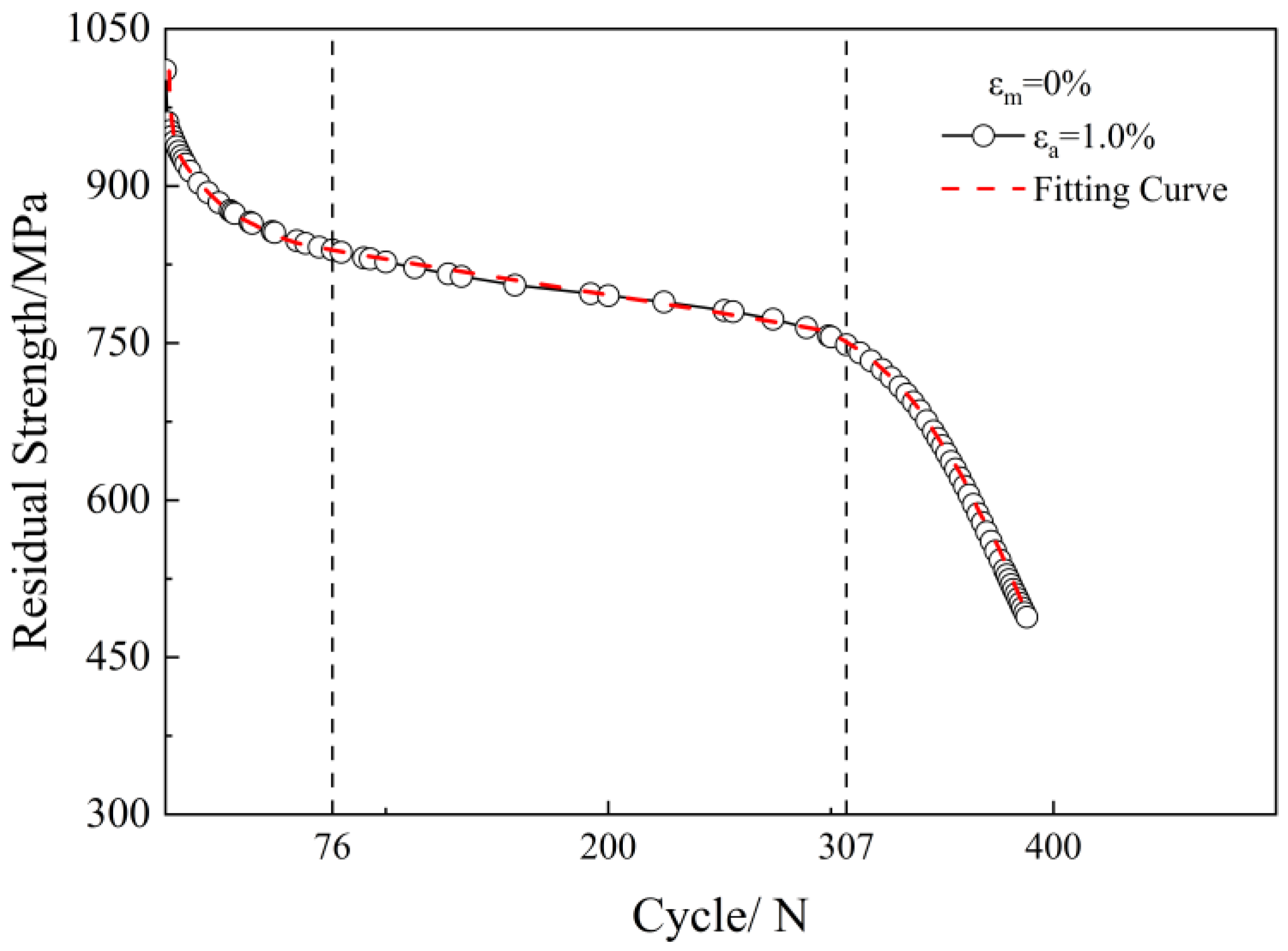
The CT110 sample used for low-cycle fatigue (LCF) tests was cylindrical. The diameter of the sample was 6 mm, and the gauge was 12 mm. Strain-controlled fatigue tests were conducted at room temperature by using a closed-loop servo hydraulic testing machine. And the tests employed tension-compression fatigue loading. In the testing, the strain amplitude was 1.0%, the mean strain was 0%, and a triangular strain waveform with the strain amplitudes was used at a constant total strain rate of 4 × 10⁻³/s [37]. The data on the peak stress of the three tests with the number of cycles were selected and averaged, and the level of uncertainty on the testing data does not exceed 5%.
It can be seen from Figure 1 that when the strain amplitude is 1.0% under symmetrical cyclic loading, the low-cycle fatigue behavior of CT110 steel has obvious cyclic softening characteristics, and its peak stress drop rate shows significant differences. The peak stress response mainly presents three stages. In the first stage, the peak stress decreases rapidly, which is about the first 20% of the entire fatigue life cycle. In the second stage, the peak stress decreases steadily, and this stage is about 20% to 80% of the whole fatigue life cycle. In the third stage, the peak stress drops rapidly to coiled tubing failure, and this stage is the last 20% of the fatigue life cycle. But for pressurized pipelines, when the peak stress of the material drops to 80% of the fatigue life cycle, the material is considered to fail. Therefore, the third stage needs to be discarded in this research.

Figure 1.
Peak stress response curve of CT110 steel.
According to the peak stress response curve of CT110 steel with a strain amplitude of 1.0%, the peak stress curves of the first stage and the second stage are fitted, respectively. Combined with the hysteretic loop model, the stress corresponding to the plastic strain of 0.2% is defined as the yield strength, and the residual yield strength models of CT110 steel at different fatigue stages can be obtained. The residual strength model is as follows [38]:
where σa1 and σa2 denote the residual yield strength of the first and second stages of damage, respectively; a, b, c, and d denote the fitting coefficients of the fitting functions for different damage stages, respectively; εa denotes the total strain amplitude; σai denotes the residual yield strength, i = 1 or 2; E denotes the elastic modulus; K′ denotes the cyclic strength coefficient; and n′ denotes the cyclic strain hardening exponent.
2.3. Residual Strength Model
First, it is necessary to determine the bending strain of each layer in the coiled tubing cross-section during the repeated bending process, then calculate the fatigue life of each layer with damage according to the strain amplitude, and finally obtain the residual strength model of the material with fatigue damage accumulation.
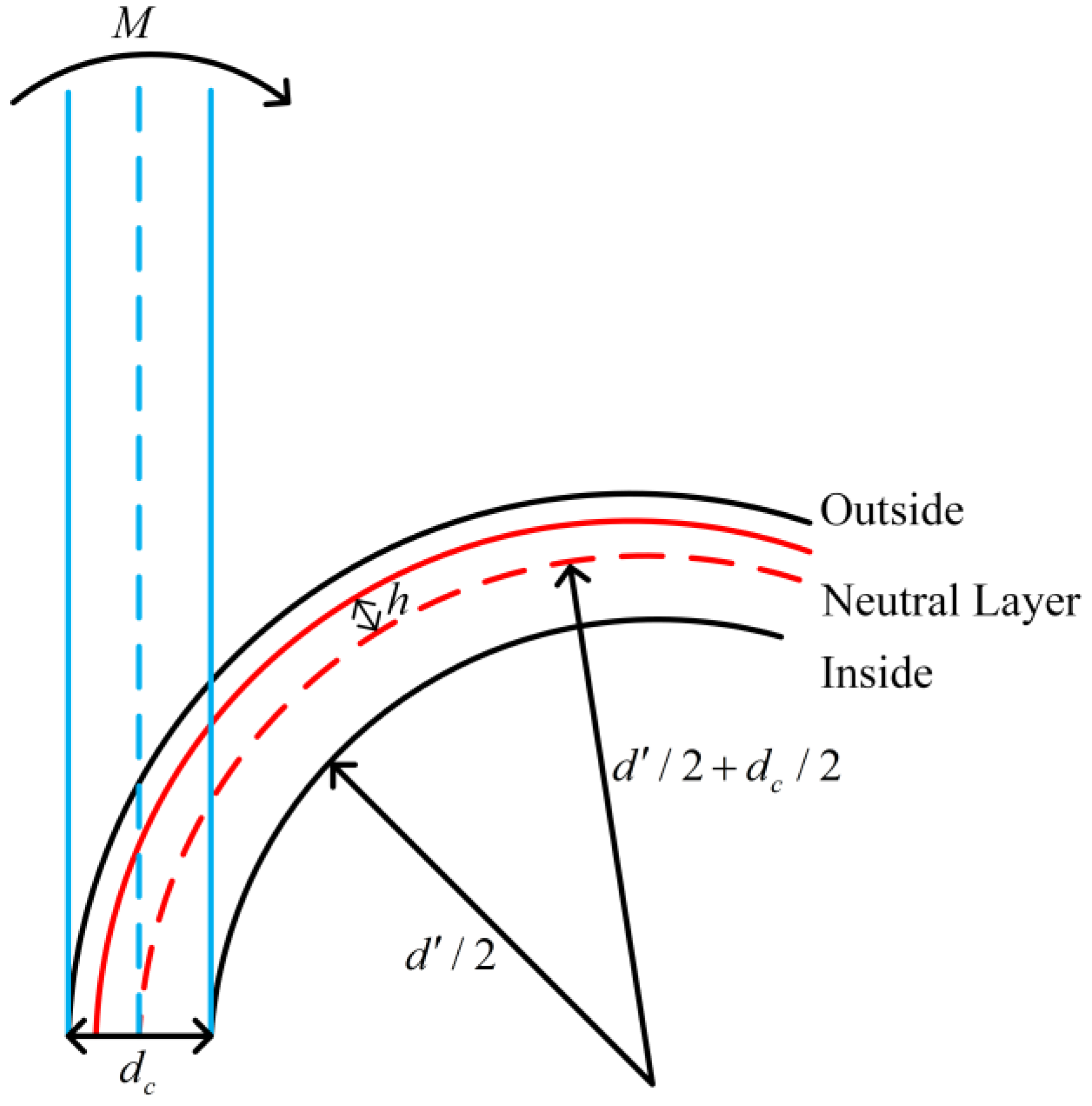
Under the action of bending moment, the coiled tubing begins to deform from the initial straight pipe state (blue straight line) toward the guide frame until it completely fits into the guide frame (black curve). The deformation process is shown in Figure 2.
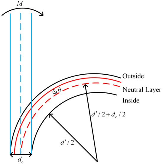
Figure 2.
Schematic diagram of coiled tubing deformation.
Assuming that the bending curvature of the coiled tubing on the drum and the guide frame is the same, the fatigue calculation of the coiled tubing can be superimposed by Miner’s law according to the constant strain amplitude. The bending strain of the coiled tubing cross-section in the vertical direction to each layer at the drum and guide frame is:
where εbh denotes the bending strain of the vertical direction of the coiled tubing section towards each layer, h denotes the deviation value between any layer and the neutral layer, dc denotes the diameter of the coiled tubing, d′ denotes the diameter of the drum and guide frame, and rb denotes the bending radius of the coiled tubing.
In particular, the maximum bending strain εbmax of coiled tubing is:
Combined Equations (1) and (4) to obtain the coiled tubing service fatigue life.
Although nonlinear fatigue damage accumulation models consider the loading sequence of different stress levels and overcome the shortcomings of linear damage accumulation models, due to their complex forms and unclear meanings in some physical models, it is difficult to determine whether the structure has experienced fatigue failure.
In addition, it has been assumed in the article that the bending radius of the pipe when bent on the drum and guide frame is the same, so there is no need to consider the loading sequence of the load. Based on the above considerations, we choose Miner’s linear damage accumulation model as the damage accumulation model for the pipe.
For the influence condition of constant strain amplitude, according to Miner’s linear damage theory, the weight of each cycle on the damage to coiled tubing material is:
where ΔDf denotes the damage amount of a single fatigue cycle and Nf denotes the fatigue life.
The number of fatigue cycles n can be determined from the damage amount of a single fatigue cycle:
where Df denotes the degree of damage to the coiled tubing.
Fitting the peak stress response curve in Figure 1 using the Belehradek function:
where σr denotes the residual strength of the material, Df denotes the damage degree of material, k denotes the function fitting coefficient, d denotes the function fitting exponent, and ΔC denotes the corrected value.
Combined with Equations (1), (3), and (4)–(7), the residual strength model of any layer of material with loading times can be established:
where εbh denotes the bending strain of any layer, equivalent to εa; h denotes the deviation value between any layer and the neutral layer; rb denotes the bending radius; Nfh denotes the fatigue life of any layer; Dfh denotes the degree of damage to any layer; n denotes the number of cycles; σrh denotes the residual strength of any layer of material; and ΔC denotes the corrected value.
The fitting parameters are shown in Table 1.

Table 1.
Residual strength model fitting coefficients.
3. Stress–Strain Analysis of Nonlinear Damaged Pipeline Structure
3.1. Research Methods and Content
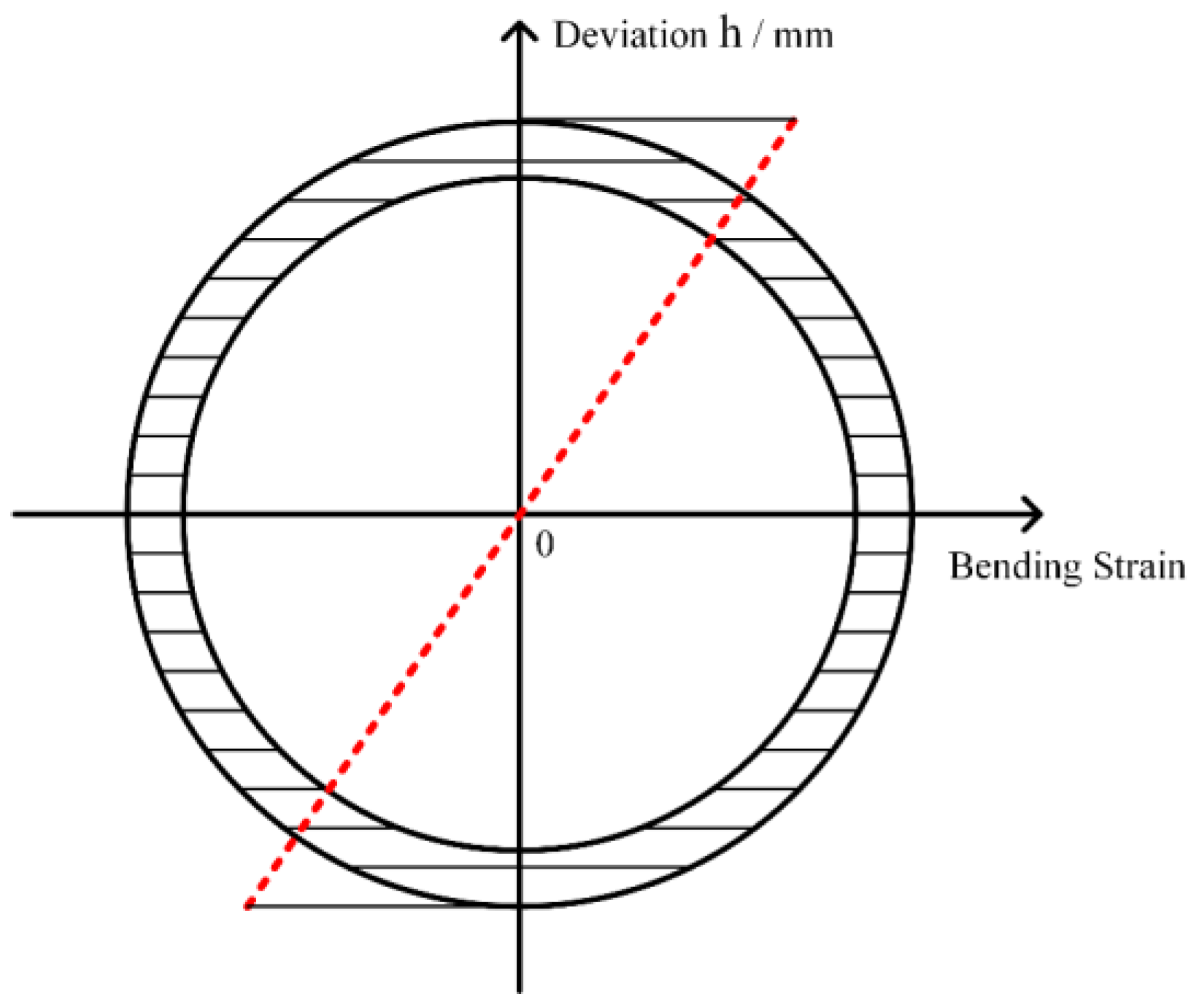
During pure bending deformation of pipe, the bending strain and bending stress on either side of the neutral layer exhibit symmetry with respect to the neutral layer, and the upper part is selected as the research object. During the “bending–straightening” alternating deformation process, the bending strain of each layer of the upper part of the neutral layer is different, resulting in nonuniform damage to the cross-section, so the residual strength of each layer of the cross-section is reduced to different degrees. According to Equation (3), the bending strain of each part can be obtained, showing a linear increasing trend from the neutral layer to the outside, and the trend is mapped to the pipe as shown in Figure 3.

Figure 3.
Variation trend of bending strain in coiled tubing section.
The section size of CT110 coiled tubing is created based on the 2-7/8” Inch coiled tubing used in the actual oil field, and the axial length is 300 mm. Dimensions and material properties are shown in Table 2.
Table 2.
Parameters of CT110.
In order to simplify the analysis, the following basic assumptions are put forward for the coiled tubing that has been run into the wellbore and has not yet been operated:
(1) The ellipticity of the coiled tubing section remains unchanged during the alternating deformation process.
(2) During the repeated bending process, there is no wear between the coiled tubing and the drum or guide frame.
To study the strength characteristics of continuous solid structures with nonuniform section damage, it is necessary to discretize the pipe in the upper part of the neutral layer. The residual strength model established in Section 2 with fatigue damage accumulation is used for stepless assignment in the vertical direction of the pipe. The damage accumulation is taken at an interval of 2% within the first 10% and at an interval of 5% between the last 10% and 80%.
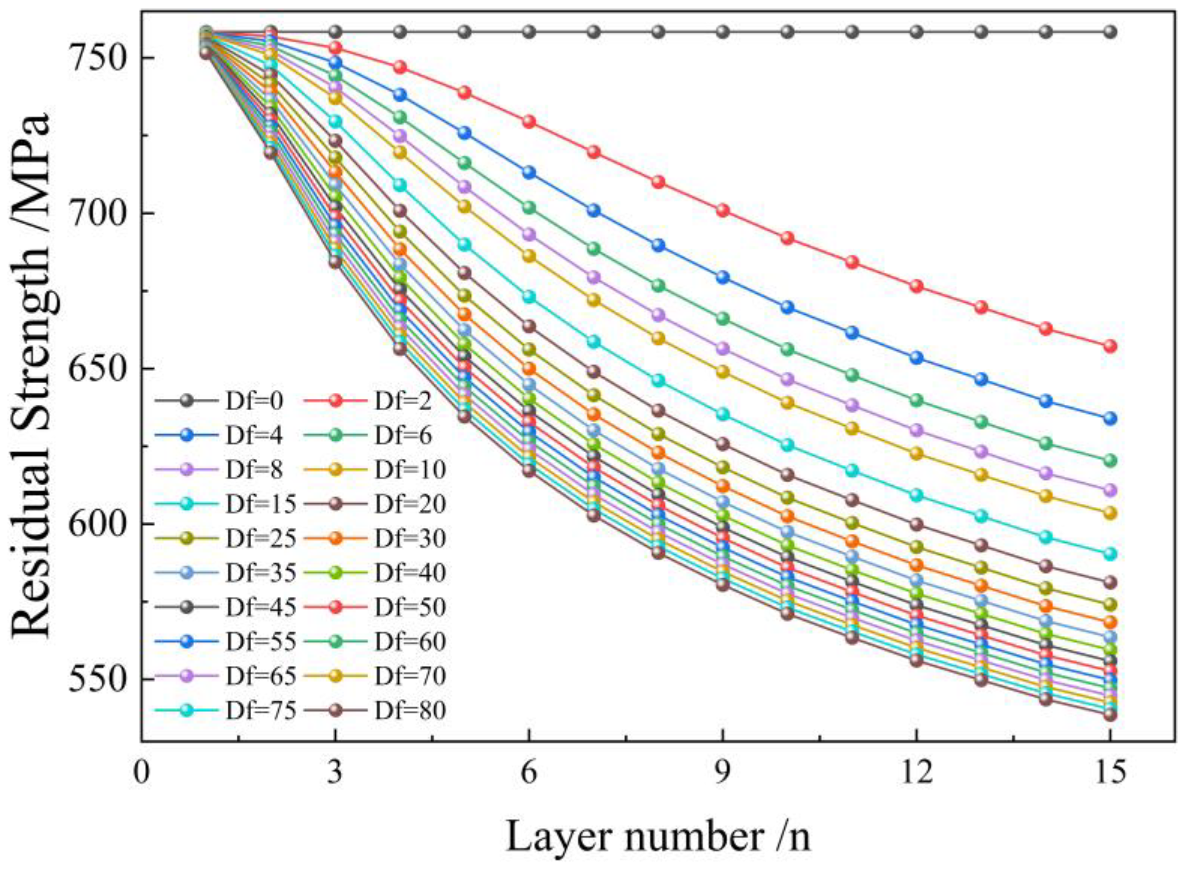
First, the bending strain εbi of each layer of the cross-section is calculated according to Equation (4), and the fatigue life Dfi of each layer can be obtained by bringing εbi into Equation (1). Combining the fatigue life Df_out of the outermost layer with Equations (5) and (6), the maximum number of repeated bendings n accumulated with damage and the single fatigue damage weight ΔDfi of each layer can be calculated. Then, combining with n and ΔDfi, the damage accumulation Dfi of each layer of the cross-section is obtained. Finally, the residual strength of each layer of the pipe cross-section accumulated with damage can be calculated by bringing the Dfi into Equation (7), as shown in Figure 4. The results show that when the damage occurs, the strength of each layer in the cross-section decreases to different degrees, showing that the residual strength of each layer decreases more with the increase in distance from the neutral layer, and the strength of the outermost layer decreases the most, with a reduction rate of 13.3%. With the accumulation of damage, the decreasing trend of the strength of each layer in the cross-section changes from rapid decreasing to slow decreasing.

Figure 4.
Residual strength of each layer under various damage degrees.
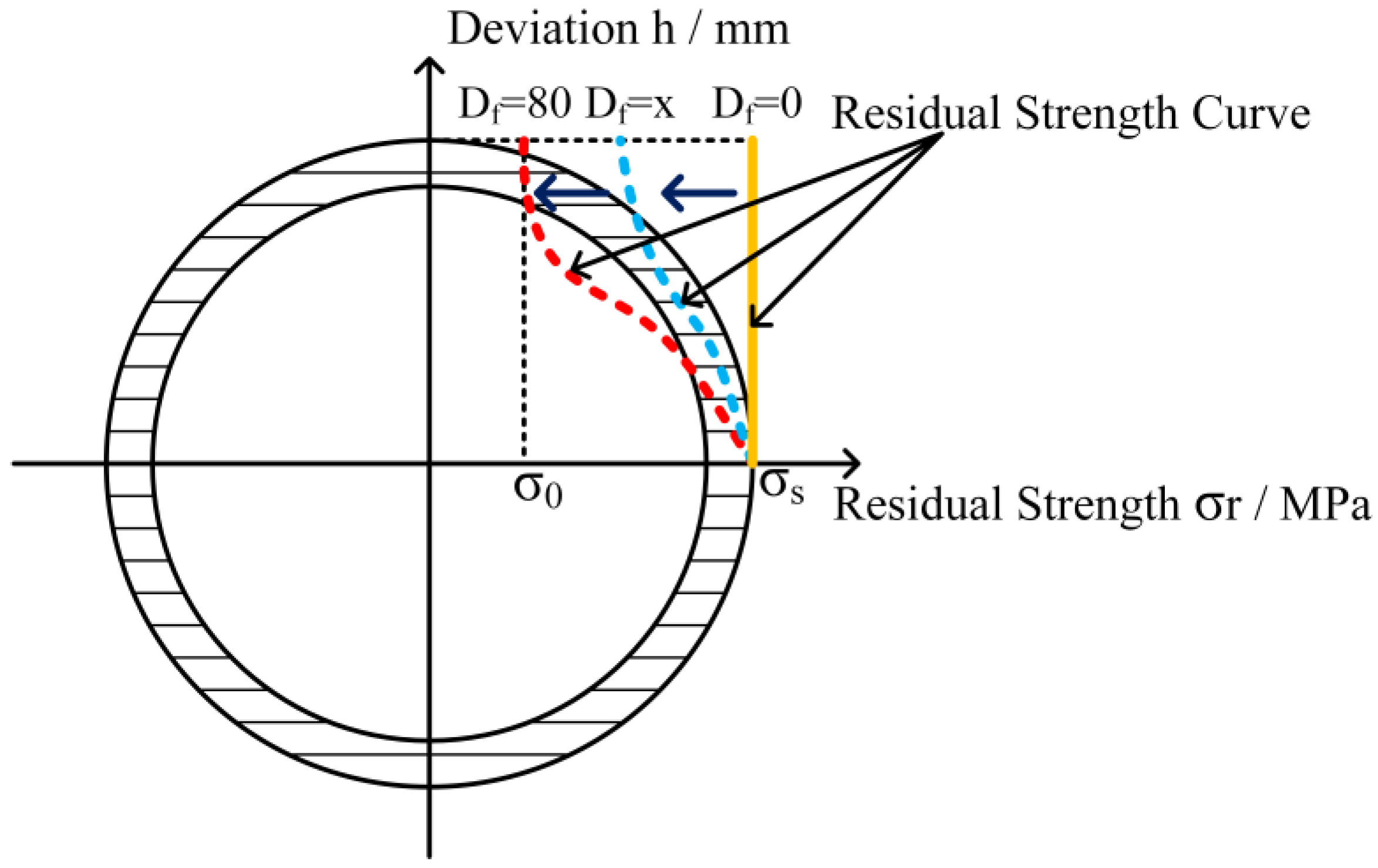
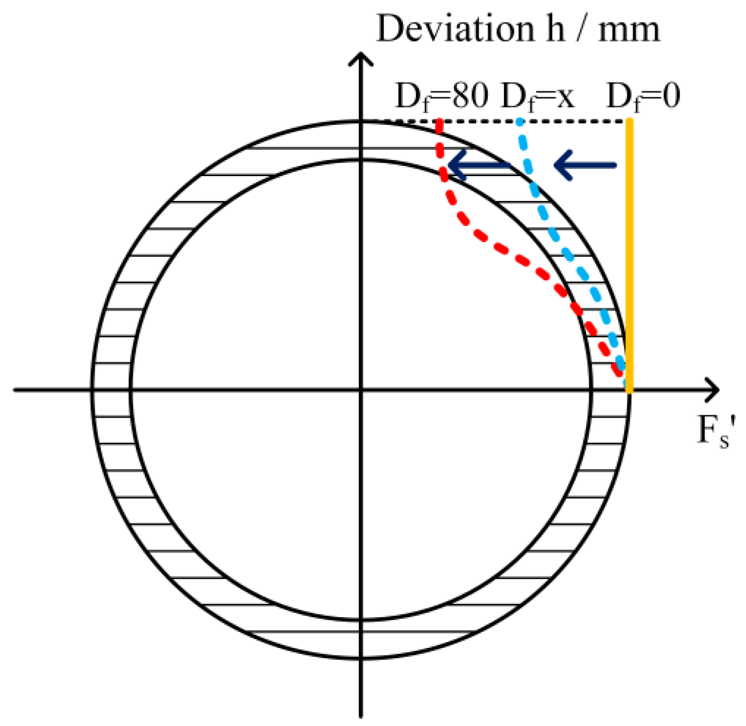
The variation trend of the residual strength of each layer element in the section is mapped to the pipe section, as shown in Figure 5, where σ0 is the residual strength of the outermost layer. When the pipe is undamaged, the residual strength remains at the initial strength (yellow line). As damage occurs, the residual strength of each layer of the section gradually decreases, and the trend transitions from the yellow line to the blue dashed curve. At this point, Df is x, 0 < x < 80. Finally, when the degree of damage to the outermost layer reaches 80%, the residual strength curve transitions from the blue-dashed curve to the red-dashed curve.

Figure 5.
Residual strength change curves.
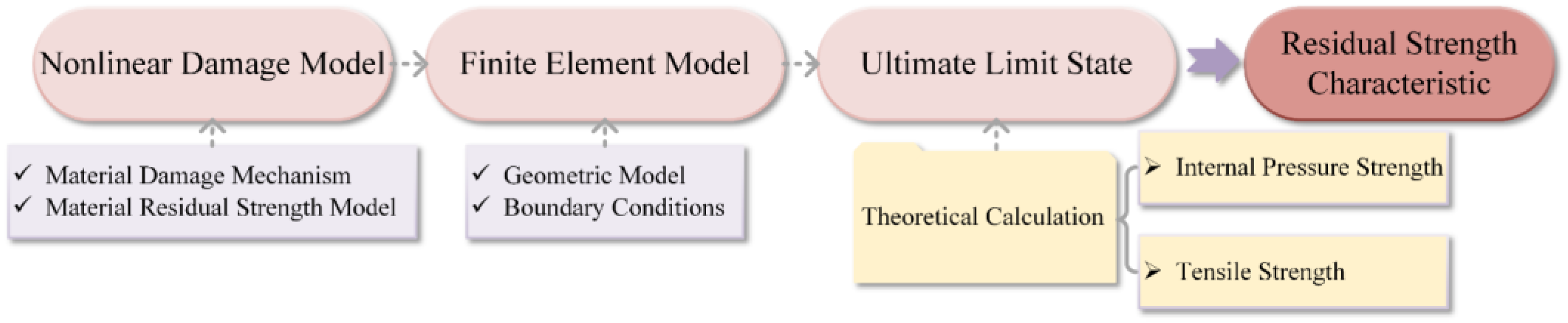
Figure 6 shows the calculation flow chart for studying the structural strength characteristics of coiled tubing with nonlinear fatigue damage, which is divided into three steps: First, according to the damage mechanism and residual strength model of the CT110 material, establish the material library of the cross-section of nonuniform damage accumulated with damage. Then, editing customized ANSYS Parametric Design Language (APDL) to assign different material strengths to each layer of the pipe, combining with the geometric model and boundary conditions, internal pressure and tensile load are applied to the nonlinear damaged pipe model, respectively, and the finite element model is solved to obtain the bearing strength of the pipe with damage accumulation. Finally, the ultimate internal pressure strength and ultimate tensile strength of the nonlinear damaged pipe are obtained by theoretical calculation, and the correctness of the finite element results is verified.
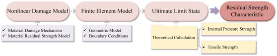
Figure 6.
Calculation flow of structural strength characteristics of nonlinear fatigue-coiled tubing.
3.2. Stress–Strain Analysis
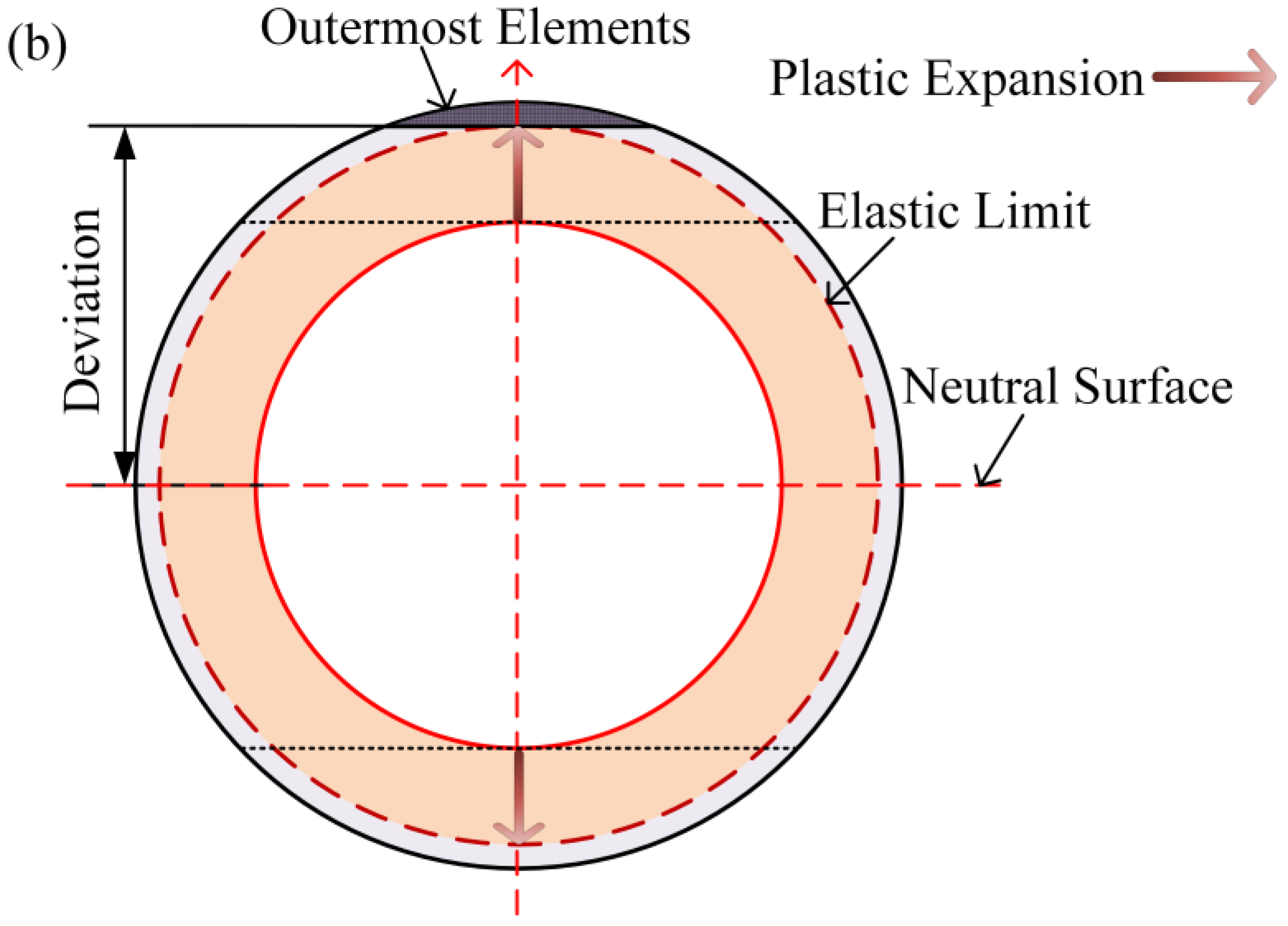
For a coiled tube without nonlinear fatigue damage, the plastic strain initially occurs on the entire inner wall annulus. As the internal pressure increases, the plastic region uniformly expands outward in a circular ring shape along the radial direction. Then, the plastic region expands to the purple-dashed ring and finally reaches the red-dashed ring. At this point, the stress on the outermost element reaches the elastic limit, as shown in Figure 7a.
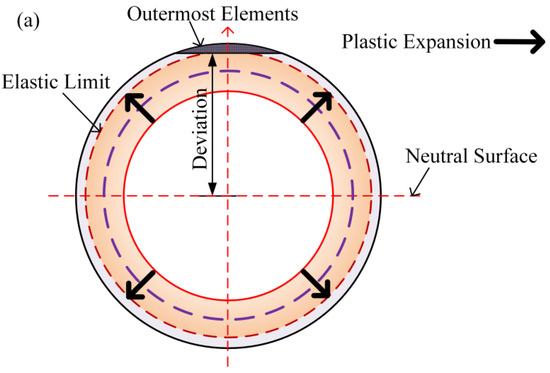

Figure 7.
Plastic strain expansion characteristics of the pipe body: (a) expanding trend of plastic strain in coiled tubing without nonlinear fatigue damage and (b) expanding trend of plastic strain in coiled tubing with nonlinear fatigue damage.
For the nonlinear fatigue-damaged pipe, the plastic strain initially occurs on the outermost inner wall in the vertical direction (the point of tangency between the black dotted line and the inner wall). As the internal pressure increases, the plastic zone expands outward in a straight line along the vertical direction until the stress of the outermost elements reaches the elastic limit, as shown in Figure 7b.
Figure 4 and Figure 5 indicate that when the degree of damage to the outermost layer reaches 80%, the nonlinear variation characteristics of the residual strength curve from the neutral layer to the outermost residual strength curve are most obvious. Therefore, the authors selected a pipe with a nonlinear damage degree of 80% to conduct stress–strain analysis on the pipe under the ultimate internal pressure condition. The solution process of ANSYS finite element software (version 2023R1) for pipes with nonuniform cross-sectional damage under internal pressure conditions is as follows:
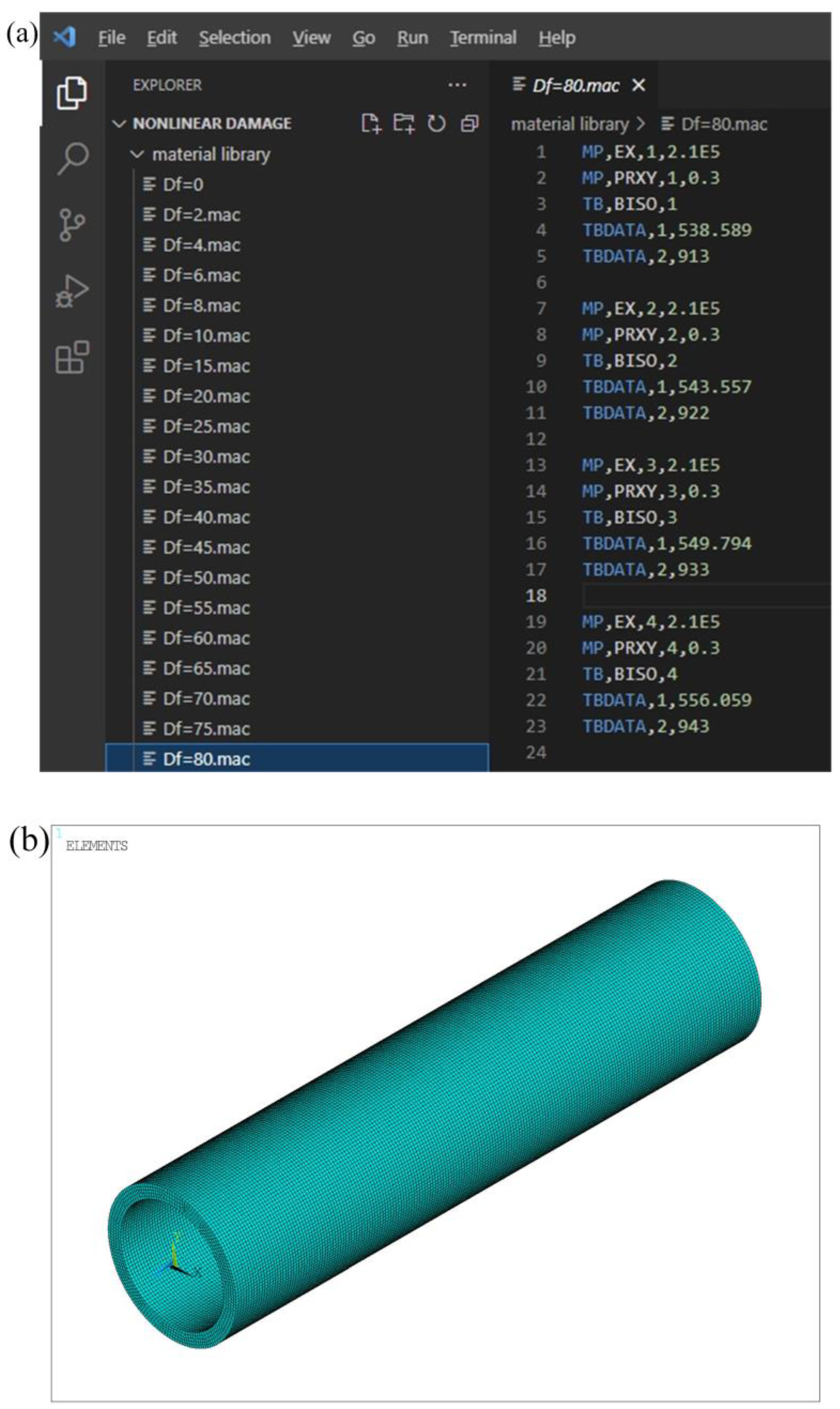
First, based on the residual strength model of CT110 coiled tubing, edit the customized APDL in Visual Studio Code software (version 1.85) to establish the material library with different degrees of damage. The hardening models of each layer are bilinear constitutive models with a yielding-to-tensile ratio of 0.8. Part of the customized APDL content is shown in Figure 8a.

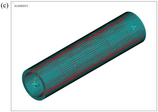
Figure 8.
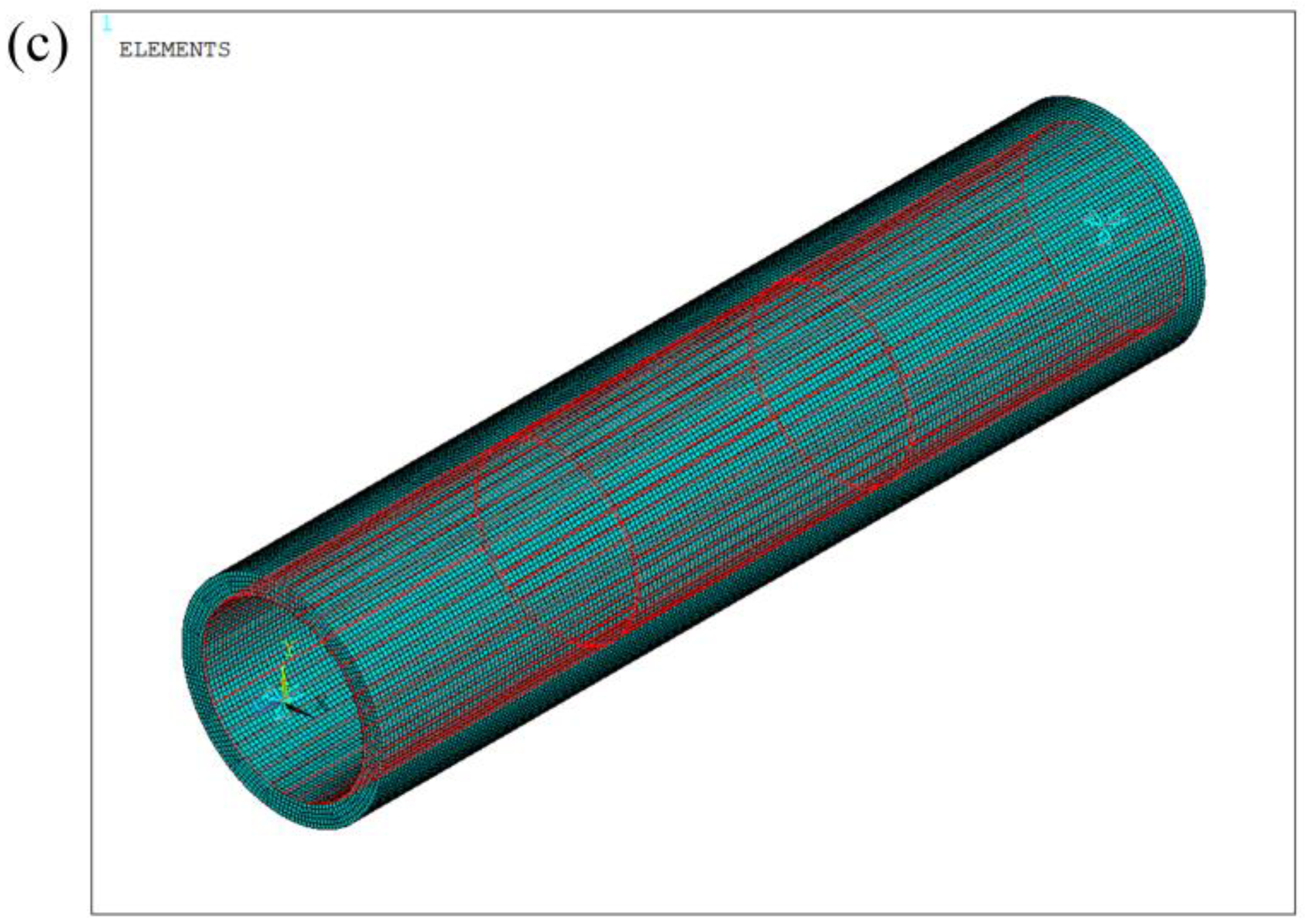
Finite element analysis process: (a) part of a customized APDL, (b) meshing result, and (c) boundary condition and static pressure load of a finite element model.
Second, establish the physical model of the pipe in ANSYS software with the sectional dimensions set in Table 2. The axial length of the pipe is 300 mm. By dissecting the physical model into a mesh with elements of size 1.5 mm, the element type is solid185, which is an eight-node hexahedral element. The model generates a total of 145,200 elements and 174,066 nodes. The meshing results are shown in Figure 8b.
Subsequently, based on the meshing result of the pipe, import the edited customized APDL with Df = 80% into the ANSYS finite element software and assign material strength to the elements of each layer of the pipe.
Finally, fixed constraint boundary conditions are applied to the two axial faces of the pipe, and a static pressure load is applied to the inner wall of the pipe to begin solving. The finite element model is shown in Figure 8c; the blue triangles represent the fixed constraint, and the red lines represent the pressure on the inner wall of the pipe.
Set the total duration of internal pressure load loading to 1 s and divide it into 10 substeps for loading, with each substep lasting 0.1 s. The full Newton-Raphson iterative method is used to solve the finite element model of the pipe. When the residual force during the iterative solution process is less than the default value of the ANSYS software program, it means that the solution is convergent. Based on this convergent solution, the iterative solution is continued until all solutions are completed and converged.
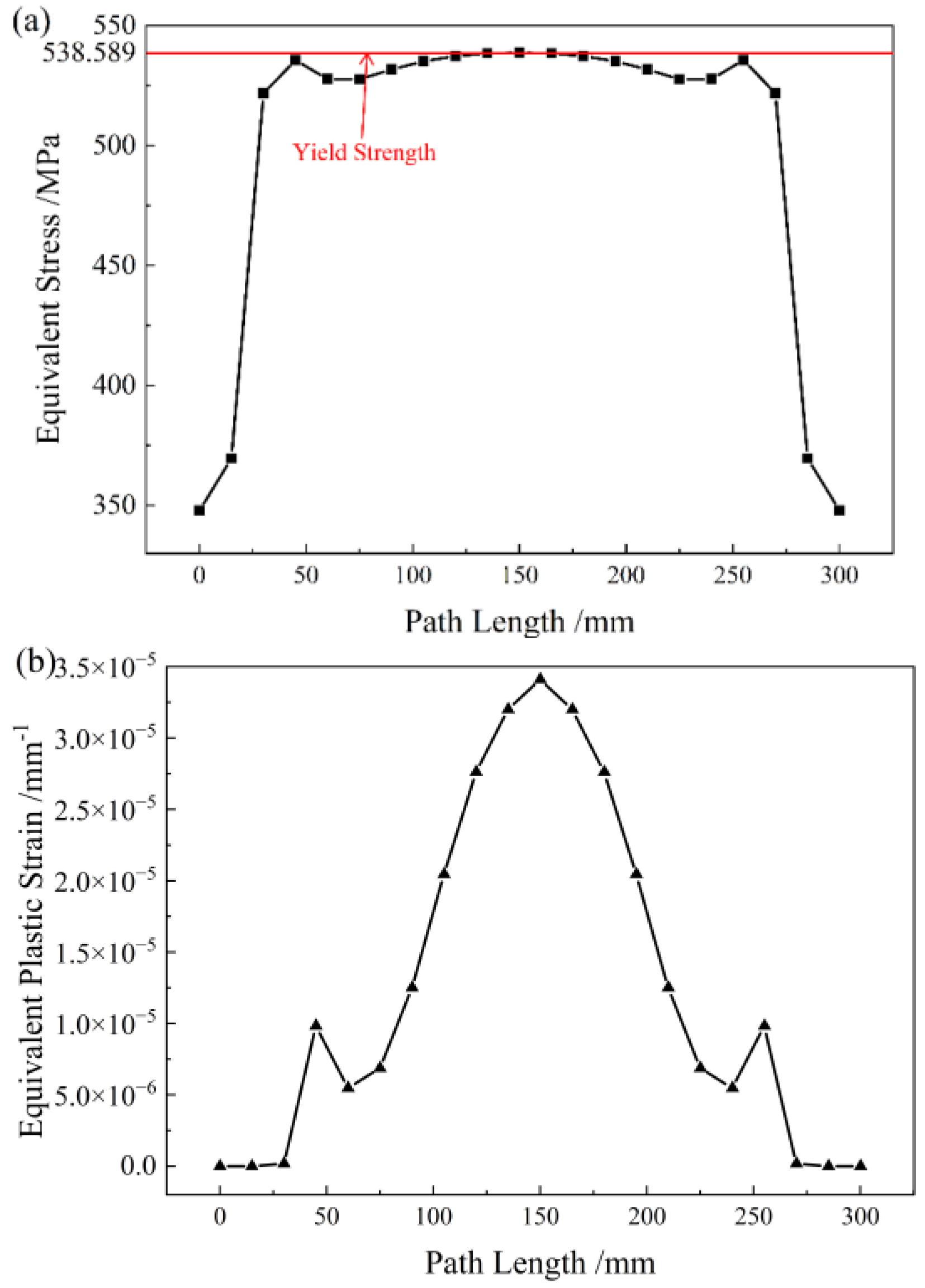
The static internal pressure load is applied to the inner wall of the pipe, causing the stress strength of the outermost elements to precisely reach yield, extracting the change curve of the equivalent von Mises stress and equivalent von Mises plastic strain of the outermost elements with the axial path, as shown in Figure 9. Since the two axial faces of the pipe are fixedly constrained, the equivalent von Mises stress in the middle section, that is, the path length of 150 mm, is the largest. Although there is an equivalent von Mises plastic strain in the outermost part of the elements, the order of magnitude is extremely small and can be ignored.

Figure 9.
Variation curve with path: (a) equivalent von Mises stress and (b) equivalent von Mises plastic strain.
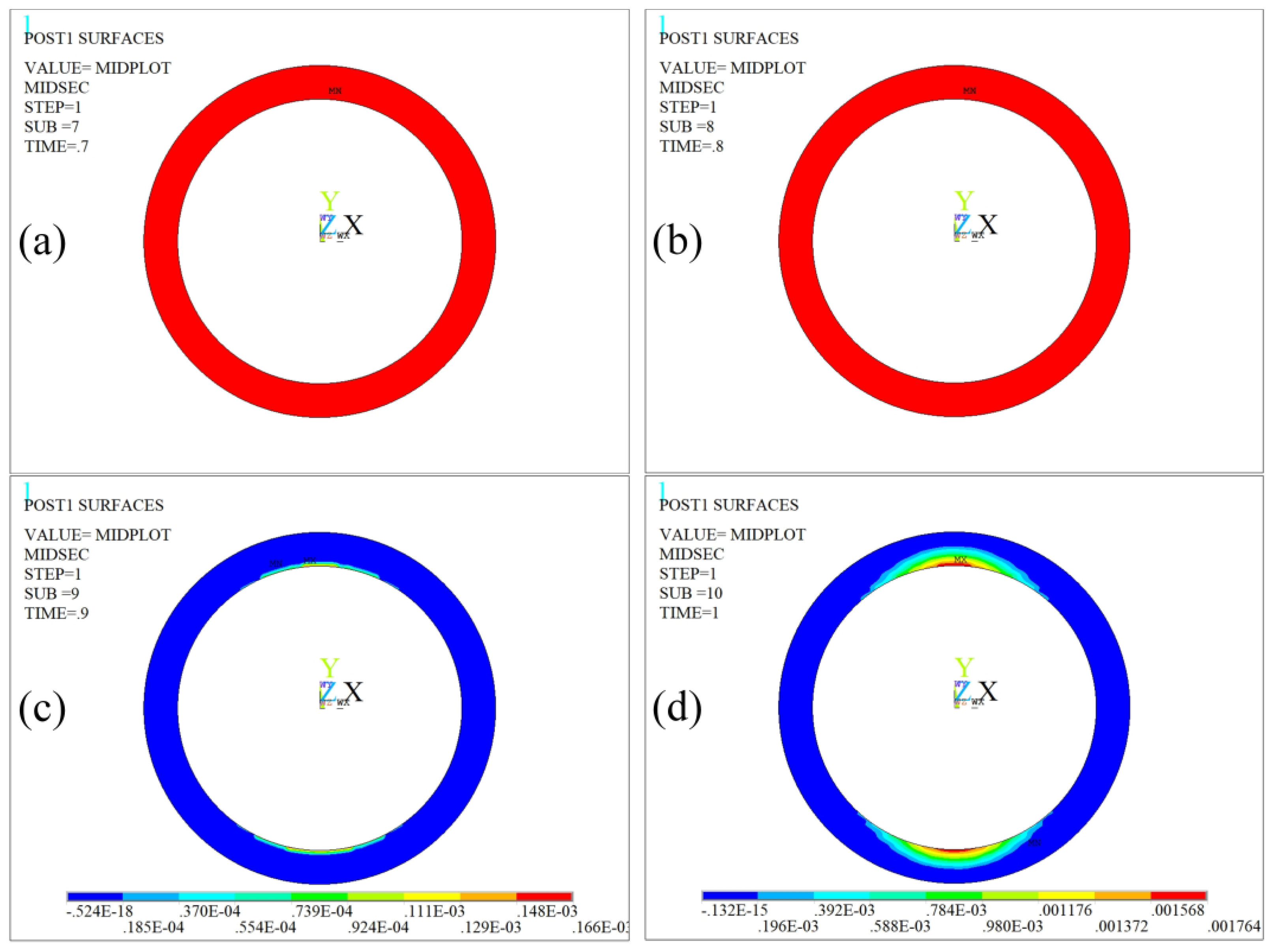
The plastic strain of the pipe cross-section at the axial path length of 150 mm is shown in Figure 10 for 0.7 s, 0.8 s, 0.9 s, and 1.0 s, respectively. The results in Figure 10 indicate that plastic strain begins to appear in the pipe at 0.9 s, and the initial plastic strain occurs on the inner wall of the pipe in the vertical direction. As the internal pressure increases, the plastic strain then expands in a straight line towards the outermost edge of the pipe until the strength of the outermost elements reaches the yield strength. The trend of the simulation results for plastic strain is consistent with the previous analysis.
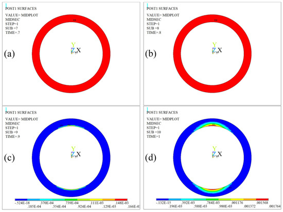
Figure 10.
Plastic strain results from pipe cross-sections at different times: (a) t = 0.7 s, (b) t = 0.8 s, (c) t = 0.9 s, and (d) t = 1.0 s.
4. Results and Discussion
4.1. Residual Strength Characteristics of the Pipe Body under the Influence of Low-Cycle Fatigue
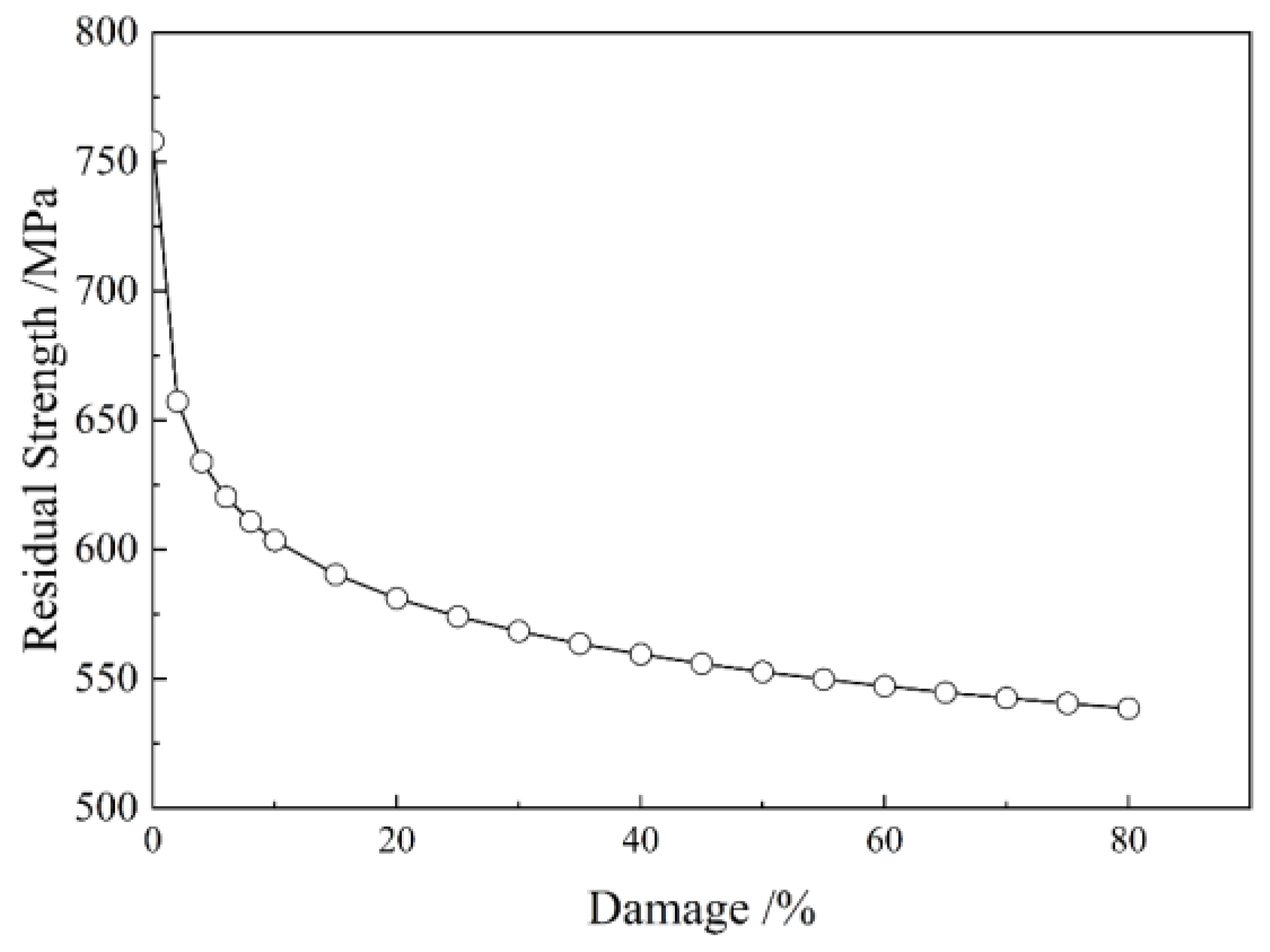
Under the influence of low-cycle fatigue after repeated “bending–straightening” alternating deformations, the strength of the CT110 steel coiled tubing material has undergone significant changes after a certain amount of damage, and the changes in the residual strength and damage degree are shown in Figure 11. When CT110 steel-coiled tubing is not damaged, the residual strength is still the initial strength of 758 MPa. When the damage level reaches 2%, the residual strength drops rapidly to 657 MPa, and the strength loss is as high as 13.3%. When the alternating deformation low-cycle fatigue is continued, the calculation results show that the residual strength of CT110 steel coiled tubing is within 20% of the damage degree, indicating a rapid decline trend. When the damage degree reaches 20%, it drops to 581 MPa, and the residual strength is 76.6% of the initial state strength. When the damage degree exceeds 20% and reaches 80%, the residual strength shows a slow and slight decline trend. The relationship between the residual strength and the damage degree in this process is approximately linear, resulting in a final residual strength loss of about 29%.

Figure 11.
Residual strength of coiled tubing with nonlinear damage.
4.2. Tensile Strength Characteristics of Nonlinear Damaged Pipe Body
After the fatigue damage occurs, according to the calculation formula for bending strain in Section 2, the ultimate load elements of different deformation layers are established, and the entire section is integrated to obtain the ultimate tensile load Fs′ of each layer of the section:
where R denotes the outer radius of the coiled tubing, r denotes the inner radius of the coiled tubing, h denotes the deviation value between any layer and the neutral layer, and σrh denotes the residual strength of any layer of material.
The variation trend of the ultimate tensile load strength of each layer element in the section is mapped to the pipe cross-section, as shown in Figure 12. The variation trend of the tensile load at each layer of the cross-section is the same as that of the residual strength of the cross-section. When the pipe is undamaged, the tensile ultimate load of each layer of the cross-section is consistent (yellow line). As damage occurs, the tensile ultimate load of each layer of the section gradually decreases, and the trend transitions from the yellow line to the blue-dashed curve. At this point, Df is x, 0 < x < 80. Finally, when the degree of damage to the outermost layer reaches 80%, the tensile ultimate load curve transitions from the blue-dashed curve to the red-dashed curve.

Figure 12.
Ultimate tensile load change curves.
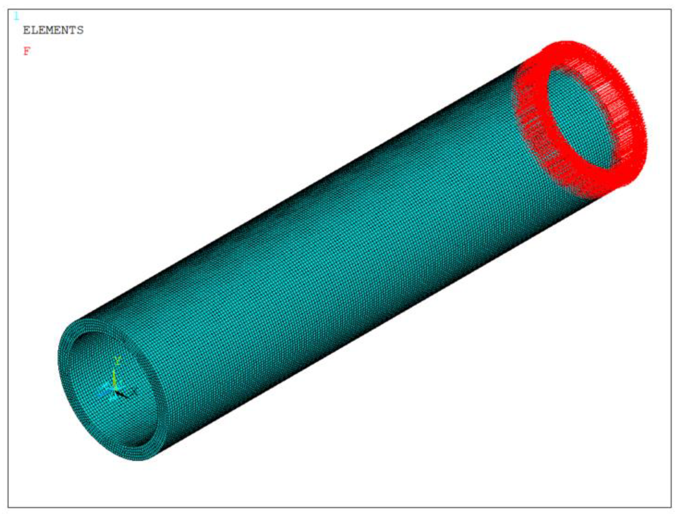
Figure 13 shows a finite element model with a fixed boundary condition at the top, where a static axial tensile load is applied at the bottom. The blue triangles represent the fixed constraint, and the red arrows represent the tensile load.

Figure 13.
Finite element model.
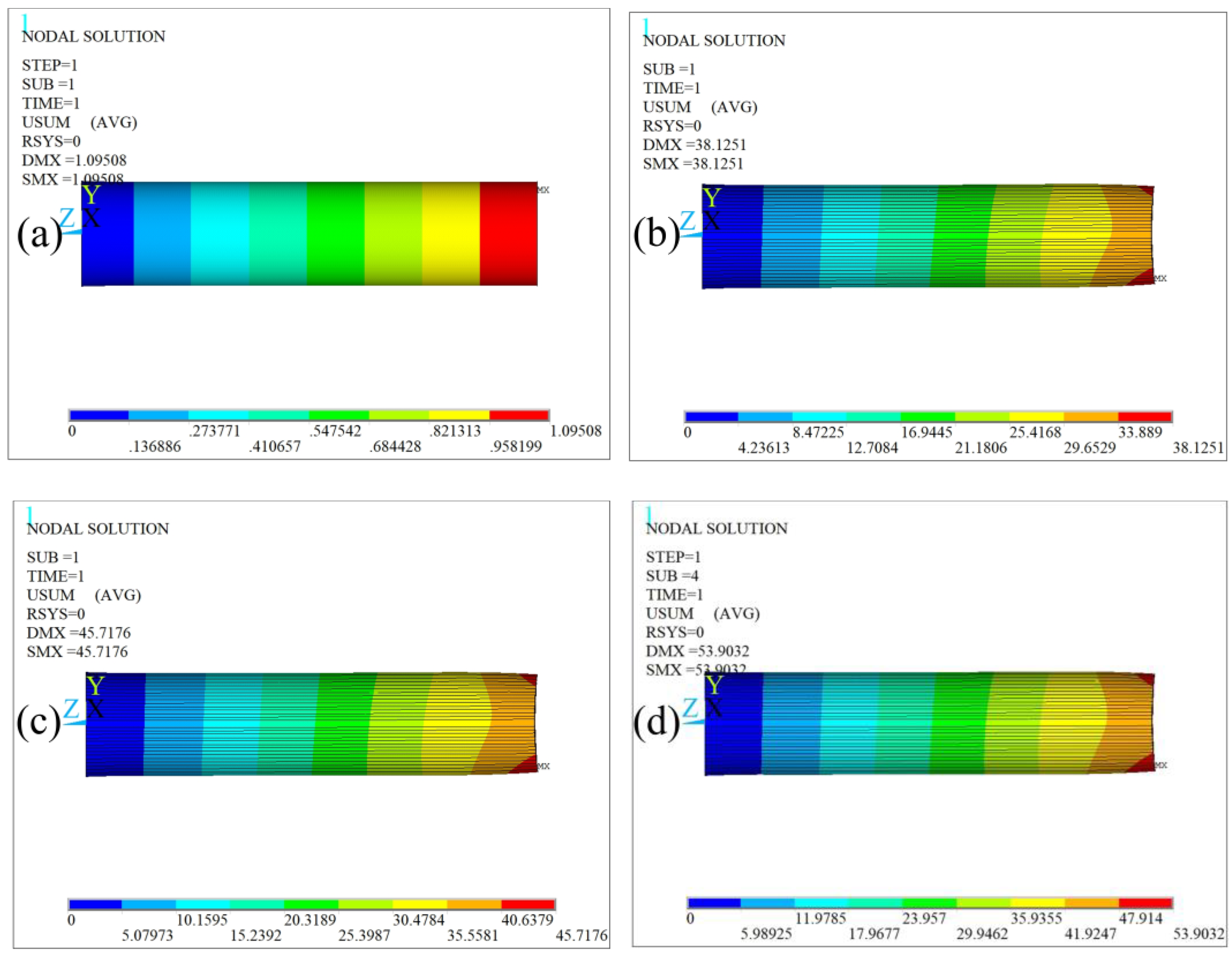
Apply tensile loads when the neutral layer enters yield to the continuous oil pipes with damage levels of 0, 20%, 40%, and 80%, respectively. The total deformation results, deformation results of the bottom, equivalent plastic strain results, and equivalent stress results of the bottom are shown in Figure 14, Figure 15, Figure 16 and Figure 17, respectively.
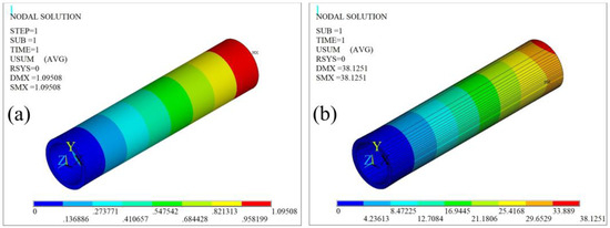
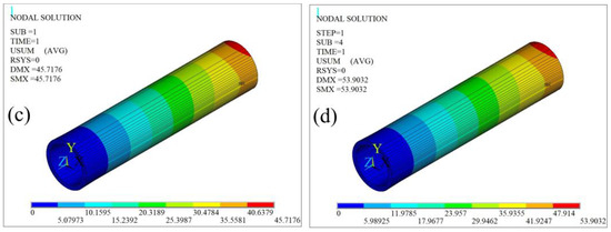
Figure 14.
Total deformation results: (a) Df = 0, (b) Df = 20%, (c) Df = 40%, and (d) Df = 80%.
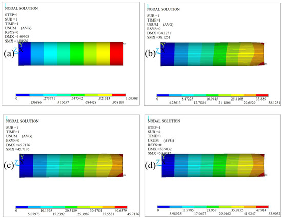
Figure 15.
Deformation results at the bottom: (a) Df = 0, (b) Df = 20%, (c) Df = 40%, and (d) Df = 80%.


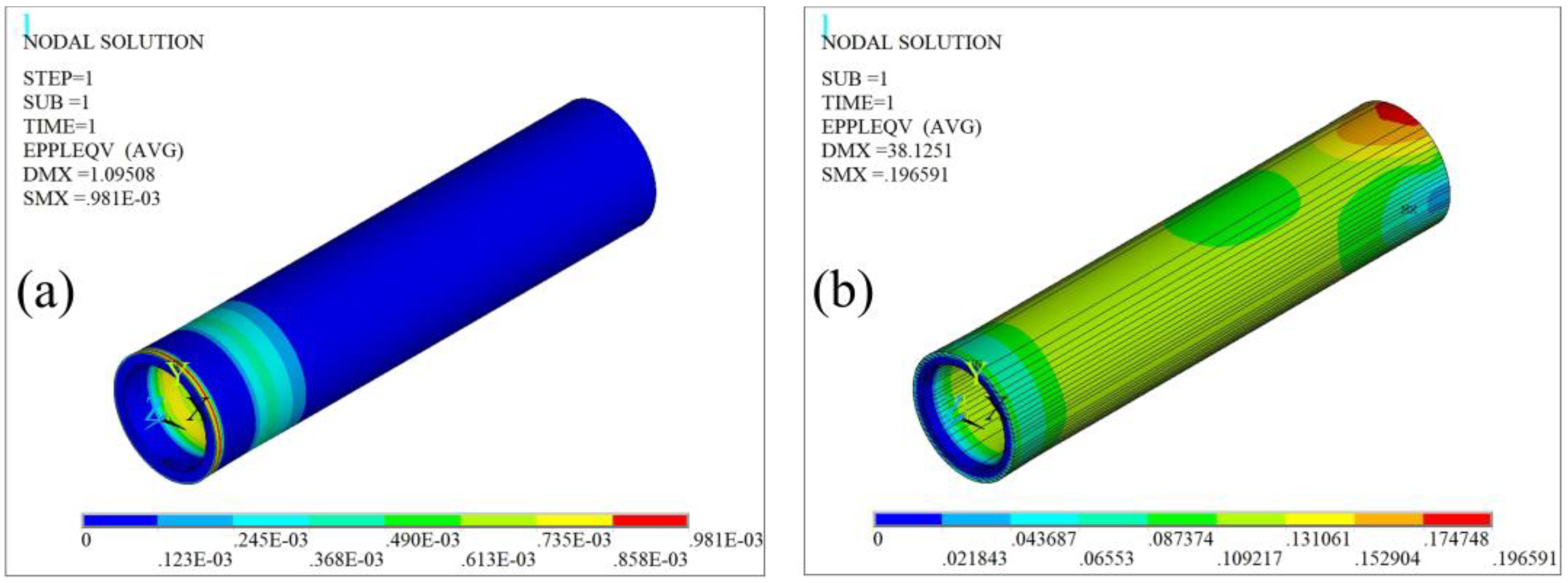
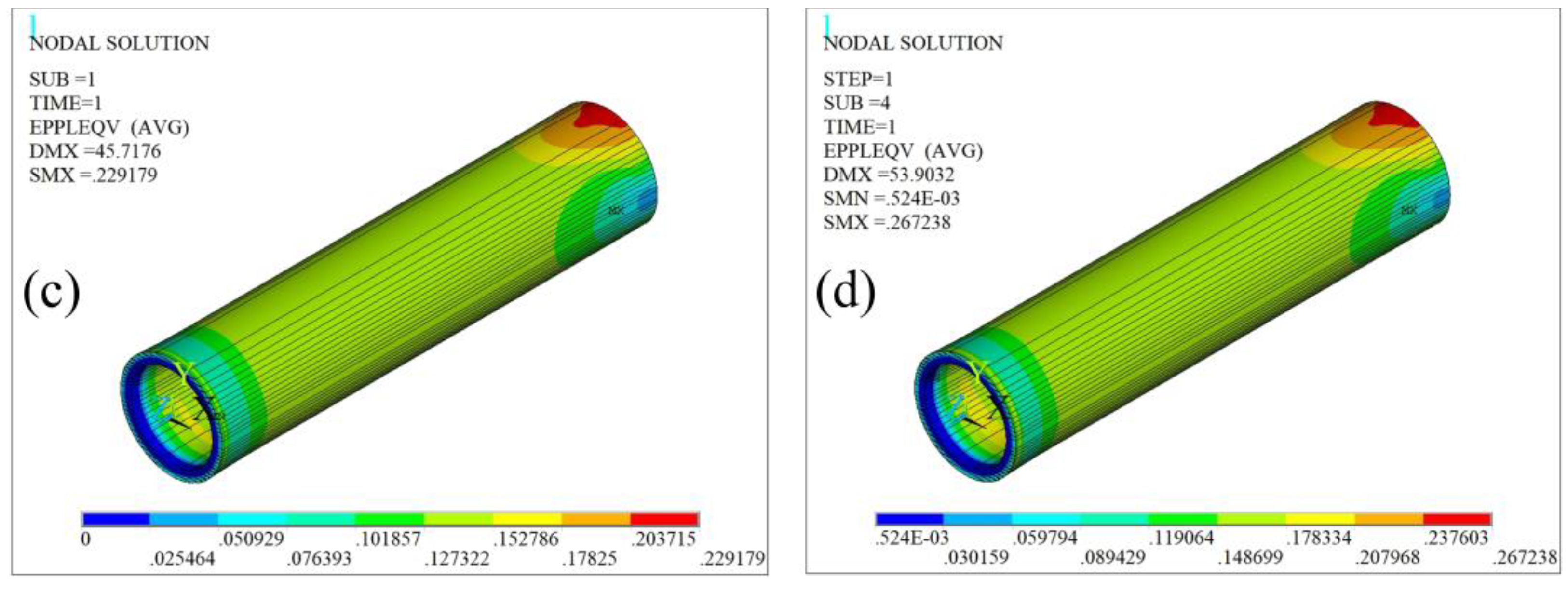
Figure 16.
Equivalent plastic strain results: (a) Df = 0, (b) Df = 20%, (c) Df = 40%, and (d) Df = 80%.
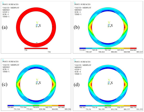
Figure 17.
Equivalent stress results at the bottom: (a) Df = 0, (b) Df = 20%, (c) Df = 40%, and (d) Df = 80%.
The results show that the tensile displacement increases with the increase in damage degree, and the deformation occurs at different positions of the bearing end, with the outermost layer having the largest deformation and the middle layer having the smallest deformation, exhibiting an inward concave characteristic. The results in Figure 16 indicate that when the strength of the neutral layer reaches the yield strength, the plastic strain on the outermost layer of the loading surface is the highest, and the plastic strain on the loading surface decreases from the outside to the inside. The explanation for this phenomenon is the following: combining Equation (9) and Figure 12, the ultimate tensile load of the cross-section shows a decreasing trend from the neutral layer to the outermost layer. As the tensile load gradually increases, the stress in the outermost layer first reaches the yield strength, and plastic strain occurs. As the load continues to increase, plastic strain also begins to appear in each layer. In addition, the stress strength of the middle layer elements is high, but the plastic strain is small. The reason is that for each layer element with approximately the same elongation, the neutral layer element finally exhibits plastic deformation due to its high residual strength.
4.3. Ultimate Internal Pressure Strength Characteristics of Nonlinear Damaged Pipe Body
It has been explained in Section 3.2 that when the stress of the outermost elements reaches the elastic limit, the internal pressure value P is considered the ultimate internal pressure strength of the nonlinear damaged pipe body. The numerical simulation of the pressure-bearing ultimate strength of the coiled tubing under each damage degree was carried out to obtain the corresponding ultimate internal pressure-bearing capacity.
The results show that the ultimate internal pressure strength and damage degree of coiled tubing show an inverse proportional trend, which can be approximately fitted by the inverse proportional function . The fitting coefficients and fitting curves are shown in Table 3 and Figure 18.
Table 3.
Fitting coefficients of bearing strength and damage degree function equation.

Figure 18.
Relationship between ultimate internal pressure strength and damage degree of coiled tubing with nonlinear damage.
4.4. Theoretical Verification of Ultimate Internal Pressure Strength
According to the maximum distortion-energy theory in material mechanics and the Lame formula for thick-walled tubing, the relationship between the theoretical ultimate internal pressure value P′ and the damage degree Df of coiled tubing with nonlinear fatigue damage is deduced:
where K denotes the ratio of the outer and inner diameters of the coiled tubing, K = R/r; R denotes the outer radius of the coiled tubing; r denotes the inner radius of the coiled tubing; hout denotes the deviation value between the outermost elements and the neutral layer; and Df denotes the degree of damage to the outermost elements.
The theoretical values of coiled tubing ultimate pressure under different damage degrees were calculated and compared with the finite element simulation values, as shown in Figure 19. The theoretical pressure-bearing value has the same variation trend as the finite element simulation value, and the theoretical value is slightly higher than the simulated value. The reasons are:
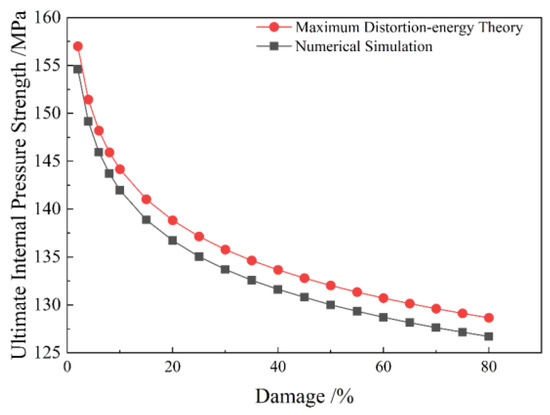
Figure 19.
Ultimate internal pressure strength of coiled tubing with nonlinear damage.
(1) The grid size divided in the finite element software is slightly larger, causing some elements in the outermost layer to cross the boundary line between the outermost edge and the second outer edge, so the theoretical value is slightly higher than the simulated value;
(2) The elements in the finite element software are divided from the inner wall to the outer wall in a circular manner, and the “stepless assignment in the vertical direction” mentioned in Section 3.1 is layered according to rectangular strips, so the theoretical value is slightly higher than the simulated value.
Due to nonlinear damage, it is difficult to calculate the residual strength of the entire structure at various locations. Therefore, the overall residual strength is usually replaced by the residual strength of the outermost layer or the residual strength of the middle layer of the upper pipe in the neutral layer in engineering. Defining “uniform damage 1” and “uniform damage 2” as follows: if we consider the degree of outermost damage as the overall degree of damage, which is called “uniform damage 1”, then the residual strength of the damaged pipe is replaced by the residual strength of the outermost layer; if we consider the damage degree of the middle layer of the upper pipe above the neutral layer as the overall degree of damage, which is “uniform damage 2”, then the residual strength of the damaged pipe is replaced by the residual strength of the middle layer of the upper pipe above the neutral layer.
Control the internal pressure to achieve the ultimate strength of the outermost elements of the structure subjected to nonlinear damage, uniform damage 1, and uniform damage 2. The maximum radial deformations of the above three types of damaged pipes are shown in Figure 20.
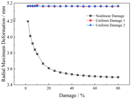
Figure 20.
Maximum radial deformation.
The results show that the maximum radial deformation of nonlinear damage pipeline structures is smaller than that of uniform damage pipeline structures, showing a rapid decrease before Df = 20% and then showing a quasi-linear slow decrease with increasing Df.
5. Conclusions
This study achieved the computability of the residual strength of nonlinear damaged pipeline structures and verified the accuracy of the theoretical load-bearing ultimate model for nonlinear damaged sections by constructing a finite element analysis model of dynamic material strength with damage. The radial deformation of nonlinear damaged and uniformly damaged pressure pipeline structures was compared. The main conclusions are summarized as follows:
(1) The residual strength and ultimate internal pressure strength of nonlinear damaged pipelines show a rapid decrease followed by a slow decrease with damage accumulation. Finally, the residual strength loss is about 29%, and the ultimate internal pressure strength decreases by about 18%. After damage, the pipeline has a heterogeneous strength structure, and the residual strength of each layer in the section decreases to varying degrees with damage accumulation, and the degree of decrease is positively correlated with its distance from the neutral layer.
(2) Under internal pressure conditions, the plastic strain of nonlinear damaged pipelines initially occurs on the inner wall in the vertical direction and then extends outward in a “straight line” form. Under tensile conditions, the tensile displacement increases with damage accumulation, and the deformation of the load-loading surface shows concave characteristics. Plastic deformation first occurs in its outermost layer and then extends towards the neutral layer.
(3) Compared to uniformly damaged pipelines, the maximum radial deformation of a nonlinear damaged pipeline under internal pressure conditions is smaller than that of a uniformly damaged pipeline.
Author Contributions
Conceptualization, W.W.; methodology, W.W.; software, R.Z. and F.F.; validation, R.Z.; formal analysis, J.C.; investigation, Y.Z.; data curation, W.W.; writing—original draft preparation, R.Z.; writing—review and editing, W.W.; visualization, Y.Z.; supervision, J.C. and Y.C.; project administration, W.W.; funding acquisition, W.W. All authors have read and agreed to the published version of the manuscript.
Funding
This research was funded by the National Natural Science Foundation of China under contact Nos. 51901180 and 52274006, the Scientific Research Program Funded by the Shaanxi Provincial Education Department under contact No. 21JP096, and the Postgraduate Innovation and Practice Ability Development Fund of Xi’an Shiyou University under contact No. YCS22212026.
Institutional Review Board Statement
Not applicable.
Informed Consent Statement
Not applicable.
Data Availability Statement
Data are contained within the article.
Conflicts of Interest
The authors declare no conflicts of interest.
References
- Wei, W.; Feng, Y.; Han, L.; Zhang, Q.; Zhang, J. Cyclic Hardening and Dynamic Strain Aging during Low-Cycle Fatigue of Cr-Mo Tempered Martensitic Steel at Elevated Temperatures. Mater. Sci. Eng. A 2018, 734, 20–26. [Google Scholar] [CrossRef]
- Wei, W.L.; Guo, L.L.; Ju, L.Y.; Han, L.H.; Feng, Y.R.; Zhang, J.B.; Zhang, Q.B. Failure Analysis and Service Life Prediction of 80SH Casing Steel under Thermal Cycle Service Environment. Mater. Sci. Forum 2020, 993, 1293–1300. [Google Scholar] [CrossRef]
- Dou, Y.; Wei, W.; Cao, Y.; Cui, L. Strengthening Mechanism of Low Cycle Fatigue Resistance for Cr-Mo Tempered Martensite Steel at 350 °C. J. Mater. Eng. Perform. 2021, 30, 2083–2090. [Google Scholar] [CrossRef]
- Shao, B.; Wang, X.; Yan, Y.; Yan, X. A Study on the Mechanical Stability of Strings of Thermal Production Wells in Steam Injection. J. Phys. Conf. Ser. 2020, 1635, 012106. [Google Scholar] [CrossRef]
- Wei, W.; Feng, Y.; Han, L.; Zhang, J.; Wang, H. High-Temperature Low-Cycle Fatigue Behavior of HS80H Ferritic–Martensitic Steel Under Dynamic Strain Aging. J. Mater. Eng. Perform. 2018, 27, 6629–6635. [Google Scholar] [CrossRef]
- Han, L.; Wang, H.; Wang, J.; Xie, B.; Tian, Z.; Wu, X. Strain-Based Casing Design for Cyclic-Steam-Stimulation Wells. SPE Prod. Oper. 2017, 33, 409–418. [Google Scholar] [CrossRef]
- Han, L.; Wang, H.; Wang, J.; Zhu, L.; Xie, B.; Tian, Z. Strain Based Design and Field Application of Thermal Well Casing String for Cyclic Steam Stimulation Production. In Proceedings of the SPE Canada Heavy Oil Technical Conference, Calgary, AB, Canada, 7 June 2016. [Google Scholar]
- Wang, J.; Yang, S.; Xue, C.; Han, L.; Wang, H. Strain Design Method for Casing Strings in Heavy Oil Thermal Recovery Well. Zhongguo Shiyou Daxue Xuebao Ziran Kexue Ban J. China Univ. Pet. Ed. Nat. Sci. 2017, 41, 150–155. [Google Scholar] [CrossRef]
- Gou, Y.; Shuang, Y.; Zhou, Y.; Cai, W.; Dai, J.; Mao, F.; Ding, X.; Zhao, C. Damage and Wall Thickness Variation of Magnesium Alloy Tube in Large Curvature and No-Mandrel Bending Process. Xiyou Jinshu Cailiao Yu Gongcheng Rare Met. Mater. Eng. 2018, 47, 2422–2428. [Google Scholar]
- Baldwin, A.J.; Hess, K.M. Mechanics of Materials. In A Programmed Review Of Engineering Fundamentals; Baldwin, A.J., Hess, K.M., Eds.; Springer: Boston, MA, USA, 1978; pp. 204–226. ISBN 978-1-4757-1223-0. [Google Scholar]
- Cheng, G.; Plumtree, A. A Fatigue Damage Accumulation Model Based on Continuum Damage Mechanics and Ductility Exhaustion. Int. J. Fatigue 1998, 20, 495–501. [Google Scholar] [CrossRef]
- Correia, J.A.F.O.; Raposo, P.; Muniz-Calvente, M.; Blasón, S.; Lesiuk, G.; De Jesus, A.M.P.; Moreira, P.M.G.P.; Calçada, R.A.B.; Canteli, A.F. A Generalization of the Fatigue Kohout-Věchet Model for Several Fatigue Damage Parameters. Eng. Fract. Mech. 2017, 185, 284–300. [Google Scholar] [CrossRef]
- Djebli, A.; Aid, A.; Bendouba, M.; Amrouche, A.; Benguediab, M.; Benseddiq, N. A Non-Linear Energy Model of Fatigue Damage Accumulation and Its Verification for Al-2024 Aluminum Alloy. Int. J. Non-Linear Mech. 2013, 51, 145–151. [Google Scholar] [CrossRef]
- Bai, S.; Li, Y.-F.; Huang, H.-Z.; Ma, Q.; Lu, N. A Probabilistic Combined High and Low Cycle Fatigue Life Prediction Framework for the Turbine Shaft with Random Geometric Parameters. Int. J. Fatigue 2022, 165, 107218. [Google Scholar] [CrossRef]
- Aid, A.; Amrouche, A.; Bouiadjra, B.B.; Benguediab, M.; Mesmacque, G. Fatigue Life Prediction under Variable Loading Based on a New Damage Model. Mater. Des. 2011, 32, 183–191. [Google Scholar] [CrossRef]
- Liao, D.; Zhu, S.-P.; Gao, J.-W.; Correia, J.; Calçada, R.; Lesiuk, G. Generalized Strain Energy Density-Based Fatigue Indicator Parameter. Int. J. Mech. Sci. 2023, 254, 108427. [Google Scholar] [CrossRef]
- Zhu, S.-P.; Liao, D.; Liu, Q.; Correia, J.A.F.O.; De Jesus, A.M.P. Nonlinear Fatigue Damage Accumulation: Isodamage Curve-Based Model and Life Prediction Aspects. Int. J. Fatigue 2019, 128, 105185. [Google Scholar] [CrossRef]
- Chin, C.H.; Abdullah, S.; Singh, S.S.K.; Schramm, D.; Ariffin, A.K. Strain Generation for Fatigue-Durability Predictions Considering Load Sequence Effect of Random Vibration Loading. Int. J. Fatigue 2023, 166, 107242. [Google Scholar] [CrossRef]
- Zhang, M.; Hu, G.; Liu, X.; Yang, X. An Improved Strength Degradation Model for Fatigue Life Prediction Considering Material Characteristics. J. Braz. Soc. Mech. Sci. Eng. 2021, 43, 275. [Google Scholar] [CrossRef]
- Hectors, K.; De Waele, W. Cumulative Damage and Life Prediction Models for High-Cycle Fatigue of Metals: A Review. Metals 2021, 11, 204. [Google Scholar] [CrossRef]
- Wang, S.; Liu, X.; Jiang, C.; Wang, X.; Wang, X. Prediction and Evaluation of Fatigue Life for Mechanical Components Considering Anelasticity-Based Load Spectrum. Fatigue Fract. Eng. Mater. Struct. 2021, 44, 129–140. [Google Scholar] [CrossRef]
- Liu, Q.; Gao, Y.; Li, Y.; Xue, Q. Fatigue Life Prediction Based on a Novel Improved Version of the Corten-Dolan Model Considering Load Interaction Effect. Eng. Struct. 2020, 221, 111036. [Google Scholar] [CrossRef]
- Huang, B.; Wang, S.; Geng, S.; Liu, X. Improved Numerical Model for Fatigue Cumulative Damage of Mechanical Structure Considering Load Sequence and Interaction. Adv. Mech. Eng. 2021, 13, 1687814021995309. [Google Scholar] [CrossRef]
- Abbasali Ayubali, A.; Prabu Shanmugavel, B.; Padmanabhan, K.A. On Material-Agnostic Fatigue Life Prediction Using Buckingham Pi Theorem. Eng. Fract. Mech. 2023, 280, 109021. [Google Scholar] [CrossRef]
- Huffman, P.J.; Beckman, S.P. A Non-Linear Damage Accumulation Fatigue Model for Predicting Strain Life at Variable Amplitude Loadings Based on Constant Amplitude Fatigue Data. Int. J. Fatigue 2013, 48, 165–169. [Google Scholar] [CrossRef]
- Subramanyan, S. A Cumulative Damage Rule Based on the Knee Point of the S-N Curve. J. Eng. Mater. Technol. 1976, 98, 316–321. [Google Scholar] [CrossRef]
- Rege, K.; Pavlou, D.G. A One-Parameter Nonlinear Fatigue Damage Accumulation Model. Int. J. Fatigue 2017, 98, 234–246. [Google Scholar] [CrossRef]
- Zhao, G.; Liu, Y.; Ye, N. An Improved Fatigue Accumulation Damage Model Based on Load Interaction and Strength Degradation. Int. J. Fatigue 2022, 156, 106636. [Google Scholar] [CrossRef]
- Araújo, L.M.; Ferreira, G.V.; Neves, R.S.; Malcher, L. Fatigue Analysis for the Aluminum Alloy 7050-T7451 Performed by a Two Scale Continuum Damage Mechanics Model. Theor. Appl. Fract. Mech. 2020, 105, 102439. [Google Scholar] [CrossRef]
- Tumanov, A.; Shlyannikov, V.N.; Zakharov, A.P. Crack Growth Rate Prediction Based on Damage Accumulation Functions for Creep-Fatigue Interaction. Frat. Ed Integrità Strutt. 2020, 14, 299–309. [Google Scholar] [CrossRef]
- Manson, S.S.; Halford, G.R. Practical Implementation of the Double Linear Damage Rule and Damage Curve Approach for Treating Cumulative Fatigue Damage. Int. J. Fract. 1981, 17, 169–192. [Google Scholar] [CrossRef]
- Hashin, Z.; Rotem, A. A Cumulative Damage Theory of Fatigue Failure. Mater. Sci. Eng. 1978, 34, 147–160. [Google Scholar] [CrossRef]
- Aeran, A.; Siriwardane, S.C.; Mikkelsen, O.; Langen, I. A New Nonlinear Fatigue Damage Model Based Only on S-N Curve Parameters. Int. J. Fatigue 2017, 103, 327–341. [Google Scholar] [CrossRef]
- Liu, Z.; Tipton, S.; Sukumar, D. Latest Development in Physics-Based Modeling of Coiled Tubing Plasticity and Fatigue. SPE J. 2022, 27, 1275–1286. [Google Scholar] [CrossRef]
- Tipton, S.M. Multiaxial Plasticity and Fatigue Life Prediction in Coiled Tubing. In Proceedings of the Advances in Fatigue Lifetime Predictive Techniques; ASTM International: West Conshohocken, PA, USA, 1993; Volume 3, pp. 283–304. [Google Scholar]
- Behenna, F.; Myrick, D.; Stanley, R.; Tipton, S.; Hammond, W. Field Validation of a Coiled Tubing Fatigue Model. In Proceedings of the SPE/ICoTA Coiled Tubing Conference and Exhibition, Houston, TX, USA, 8–9 April 2003. [Google Scholar] [CrossRef]
- Wei, W.; Han, L.; Wang, H.; Wang, J.; Zhang, J.; Feng, Y.; Tian, T. Low-Cycle Fatigue Behavior and Fracture Mechanism of HS80H Steel at Different Strain Amplitudes and Mean Strains. J. Mater. Eng. Perform. 2017, 26, 1717–1725. [Google Scholar] [CrossRef]
- Ellyin, F. Cyclic Stress-Strain Response. In Fatigue Damage, Crack Growth and Life Prediction; Ellyin, F., Ed.; Springer: Dordrecht, The Netherlands, 1997; pp. 33–76. ISBN 978-94-009-1509-1. [Google Scholar]


Disclaimer/Publisher’s Note: The statements, opinions and data contained in all publications are solely those of the individual author(s) and contributor(s) and not of MDPI and/or the editor(s). MDPI and/or the editor(s) disclaim responsibility for any injury to people or property resulting from any ideas, methods, instructions or products referred to in the content. |
© 2024 by the authors. Licensee MDPI, Basel, Switzerland. This article is an open access article distributed under the terms and conditions of the Creative Commons Attribution (CC BY) license (https://creativecommons.org/licenses/by/4.0/).