
Study on the Time Domain Semi Analytical Method for Horizontal Vibration of Pile in Saturated Clay
Abstract
:1. Introduction
2. Mechanical Model
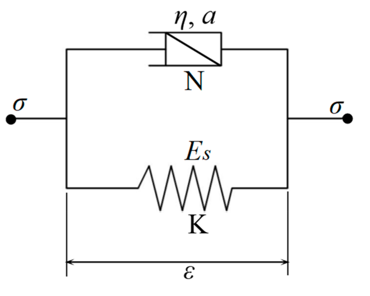
2.1. Fractional Order Kelvin Model
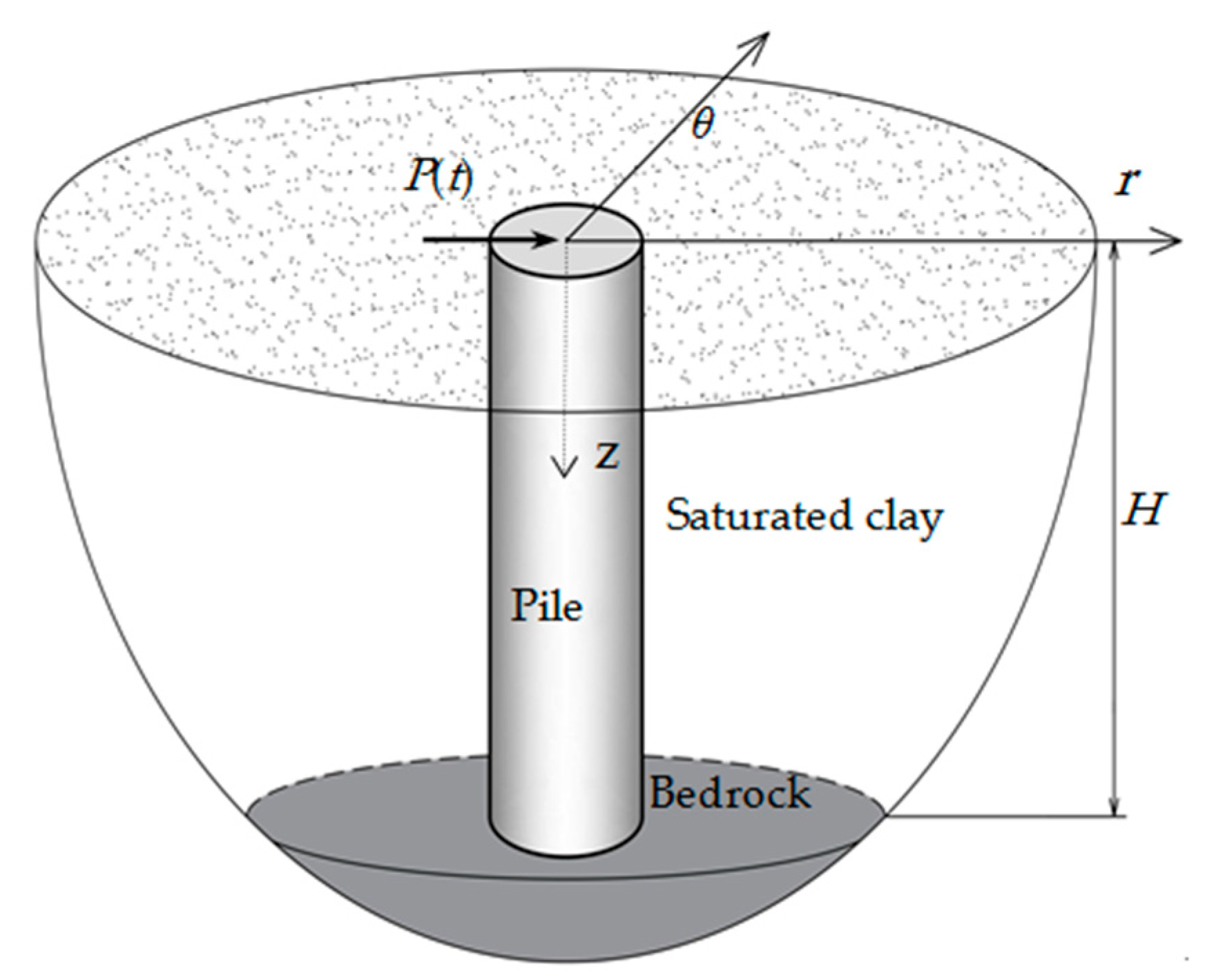
2.2. Horizontal Coupled Vibration Model of Pile Soil
3. Equation Solving
3.1. Solving the Control Equation of Saturated Clay Movement
3.2. Solution of Pile Foundation Vibration Equation
4. Example Analysis
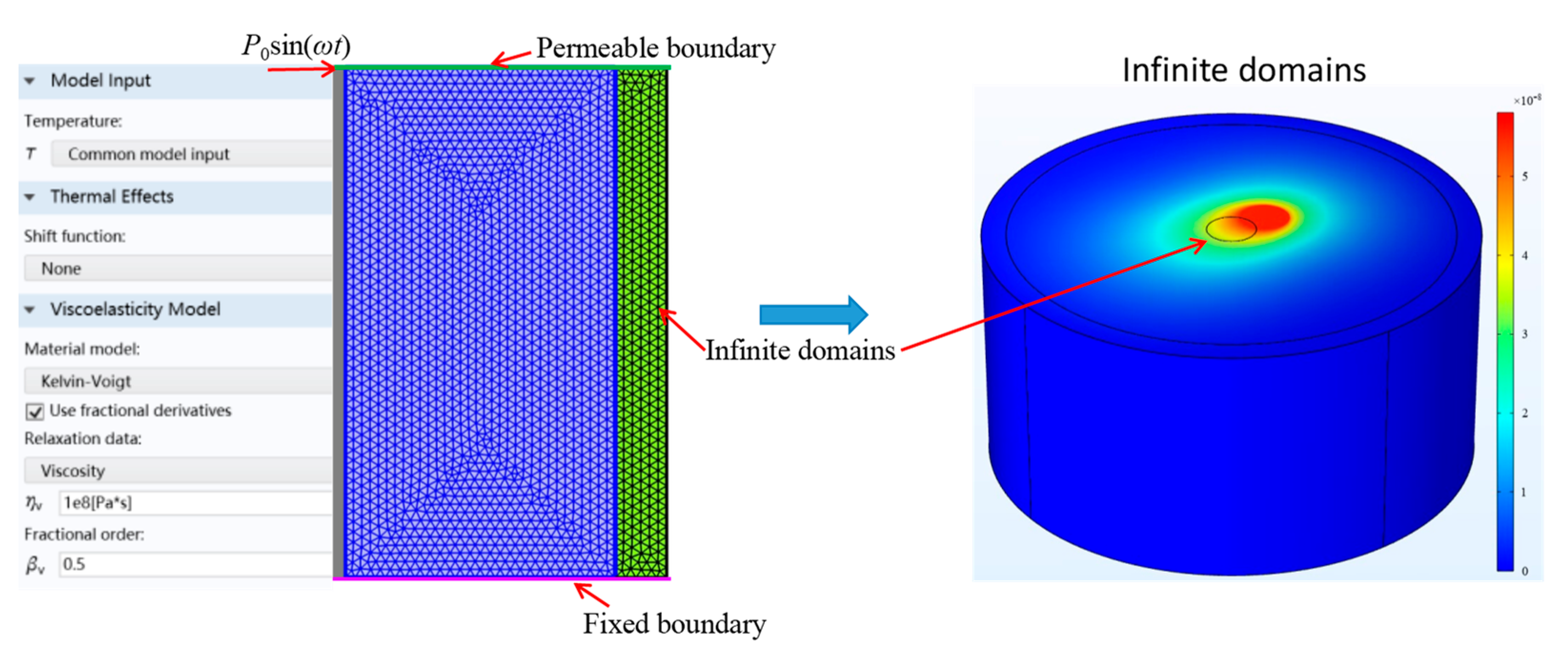
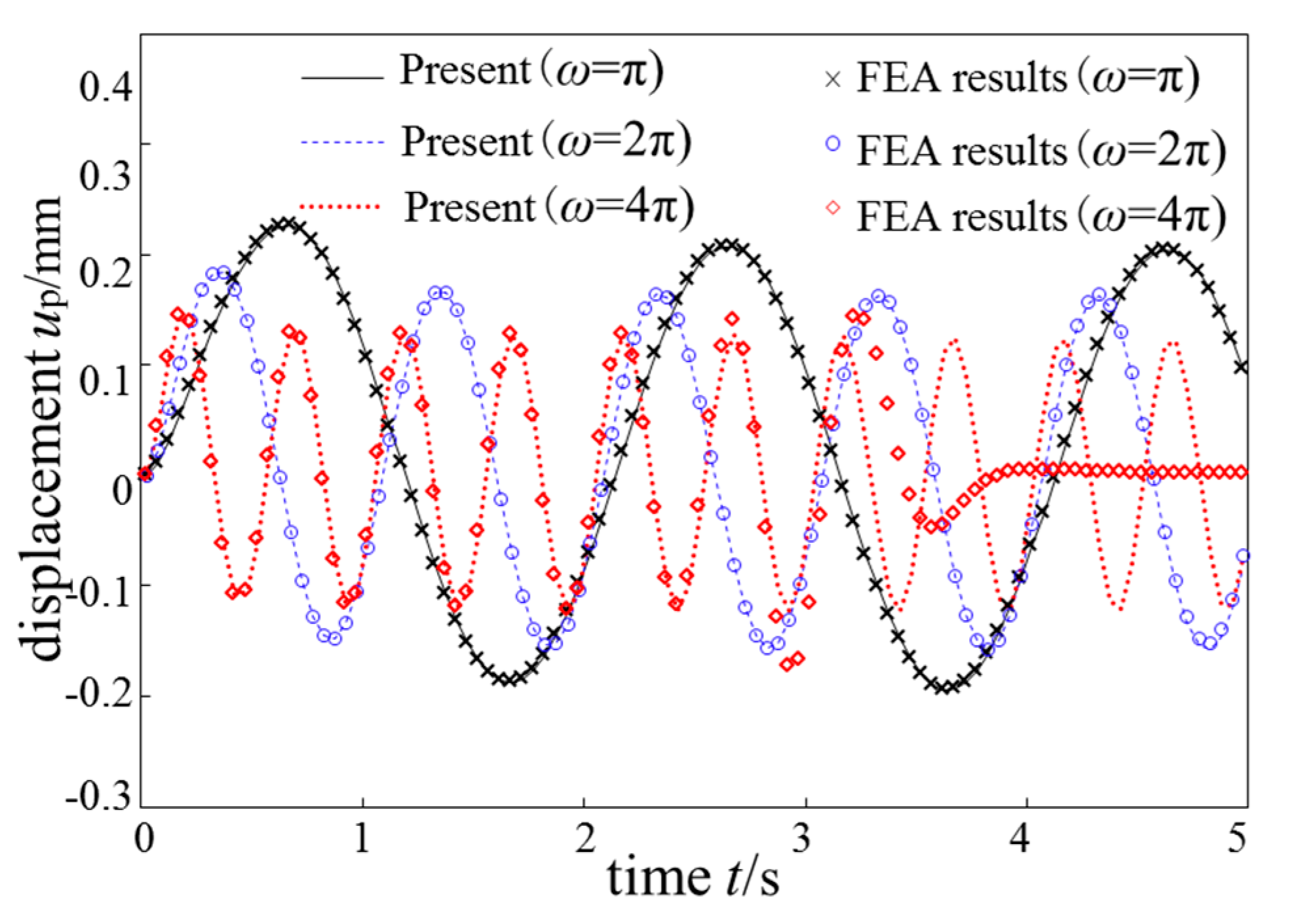
4.1. Algorithm Verification
4.2. Pile Foundation Vibration Analysis
5. Conclusions
- (1)
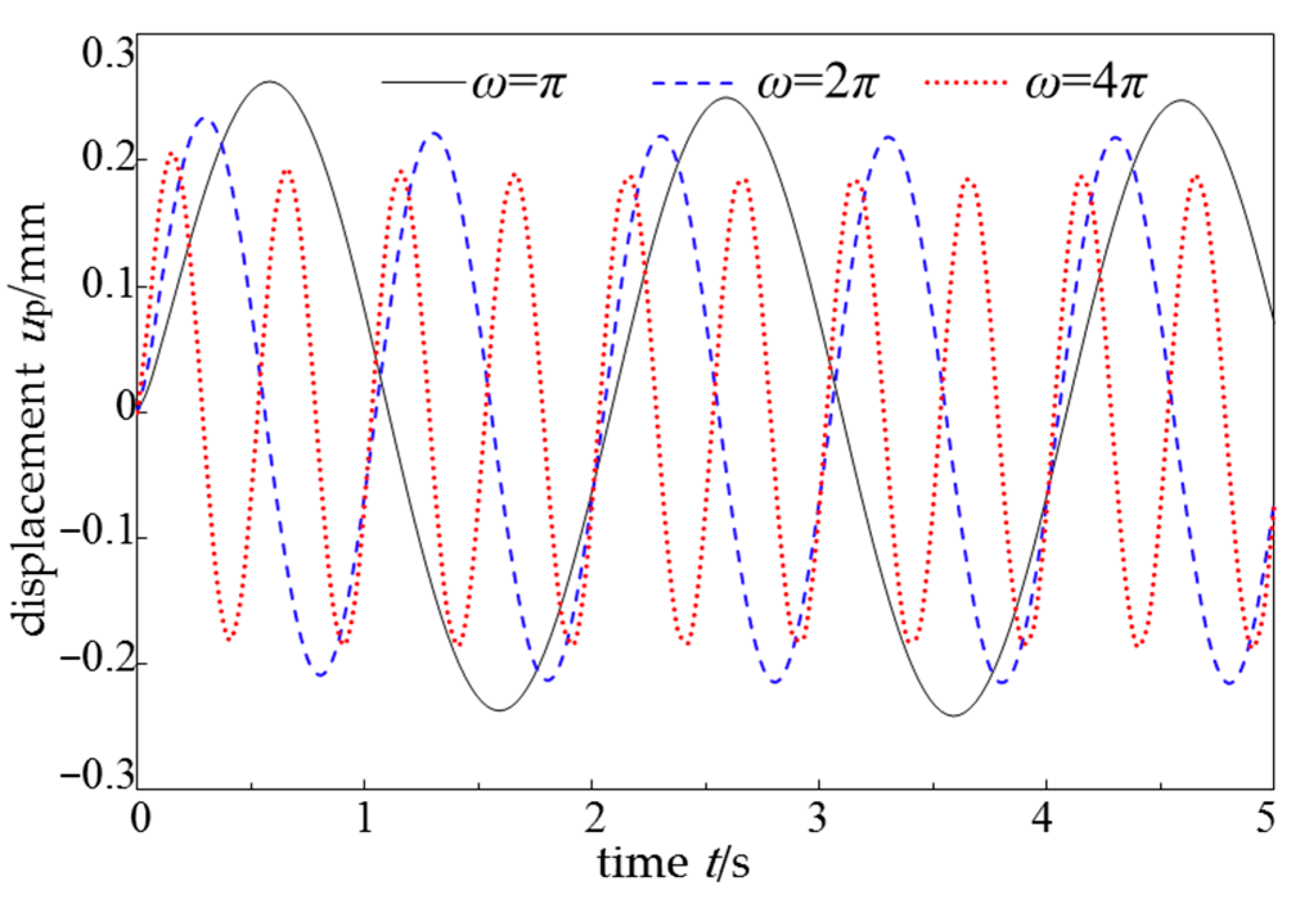
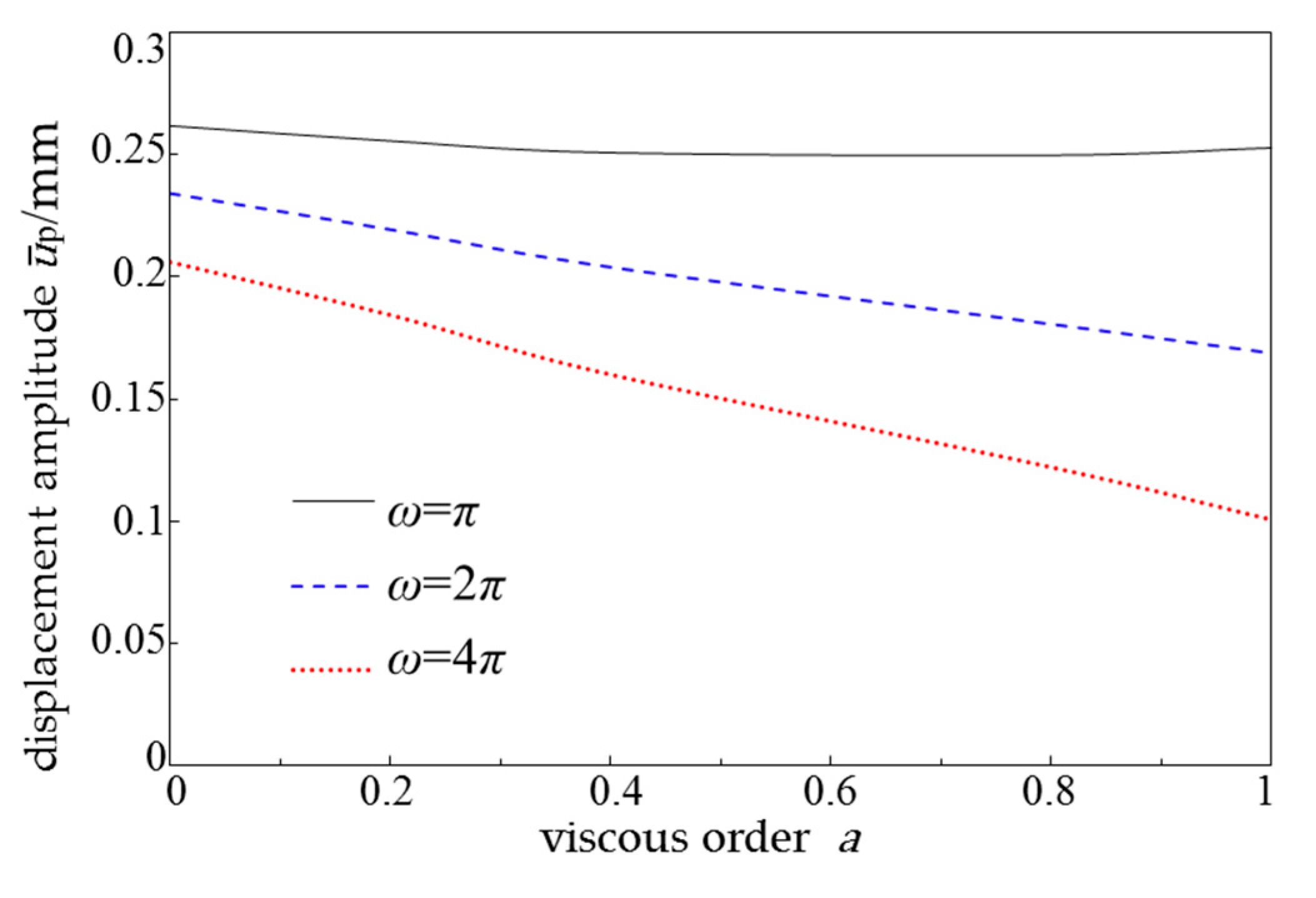
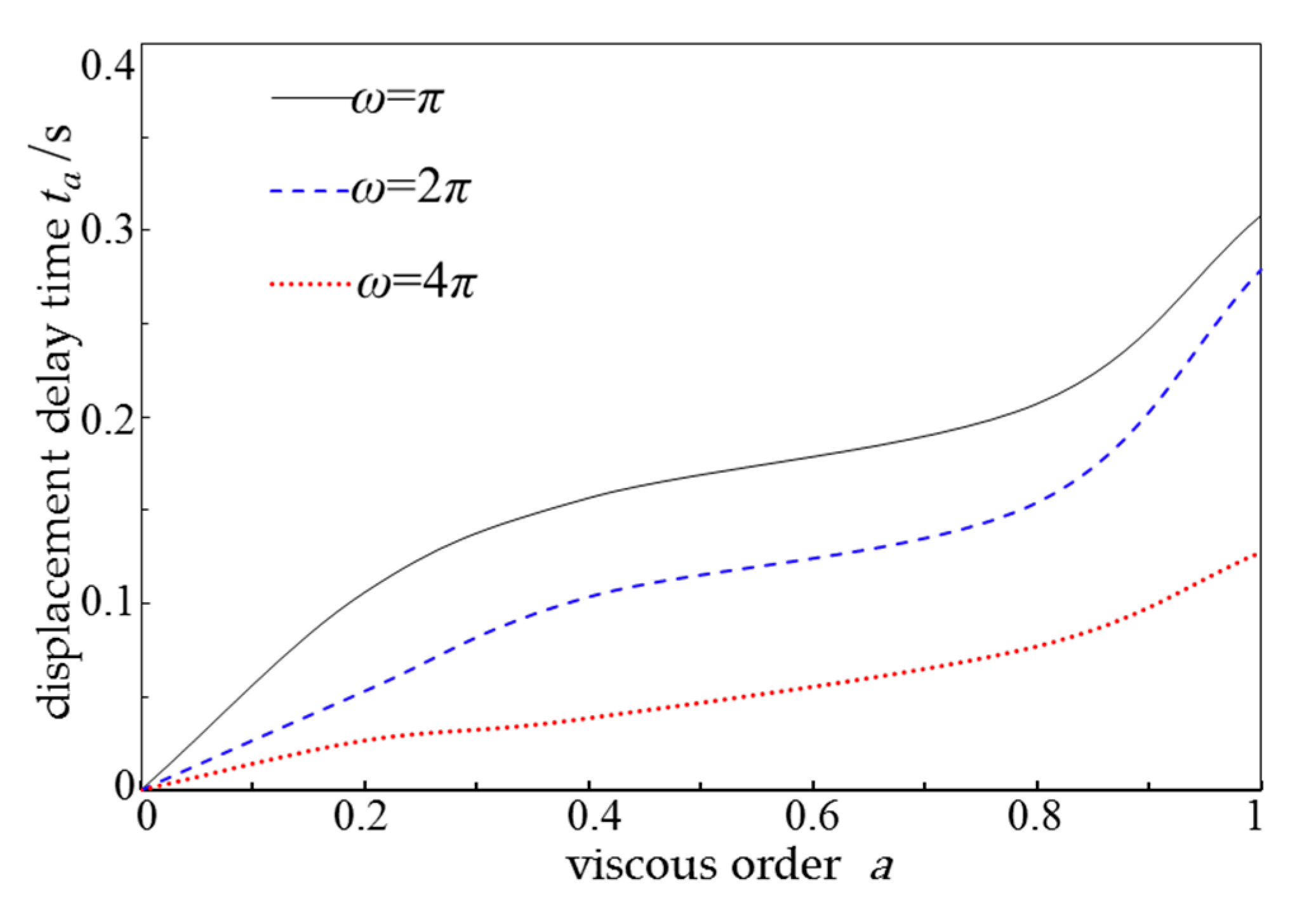
- The displacement and internal force response of pile vibrations in saturated clay foundations have a delayed effect. The stronger the rheological properties of the foundation soil, the more obvious the delay, and the lower the load frequency, the more significant the influence of rheological properties on the delay effect.
- (2)
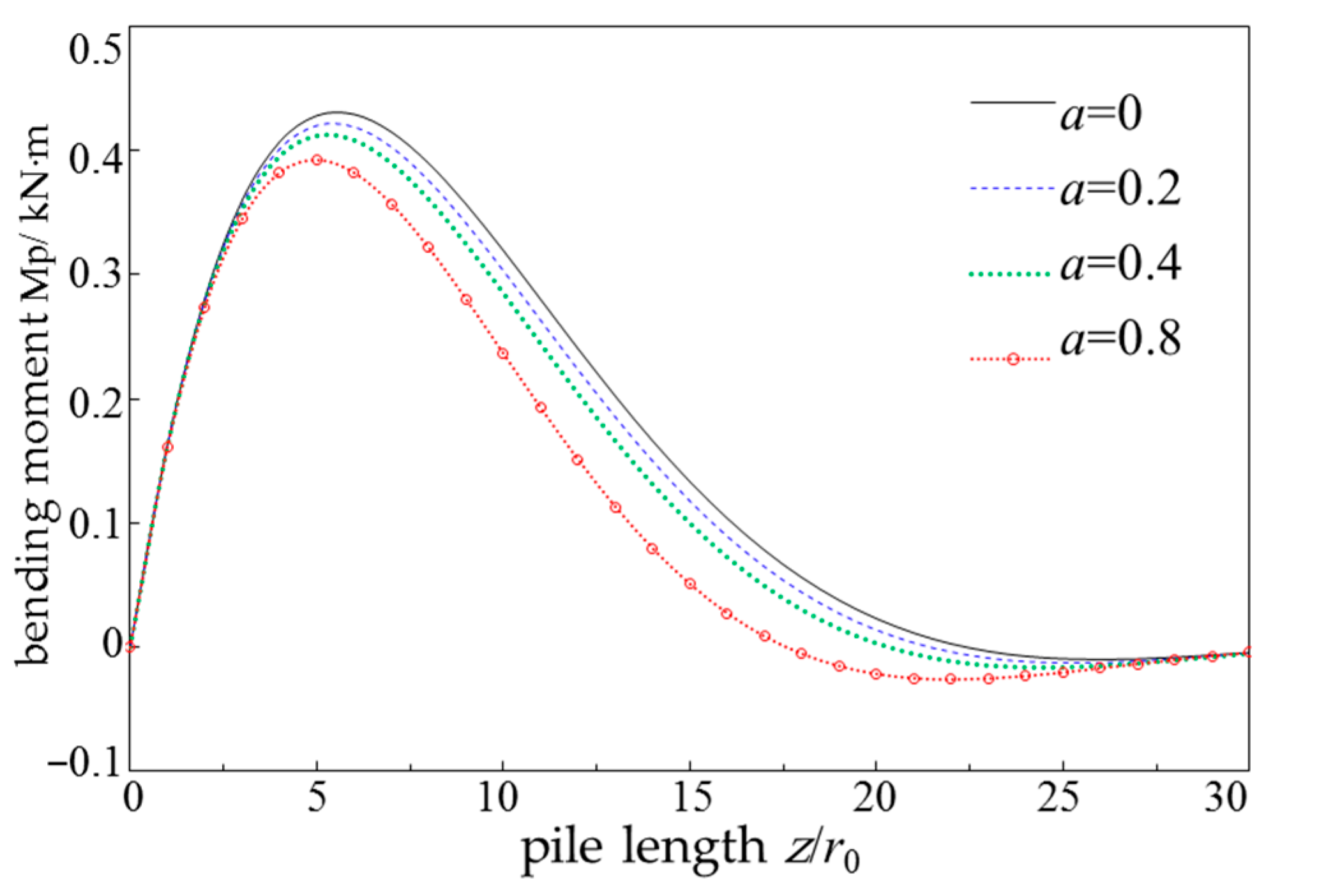
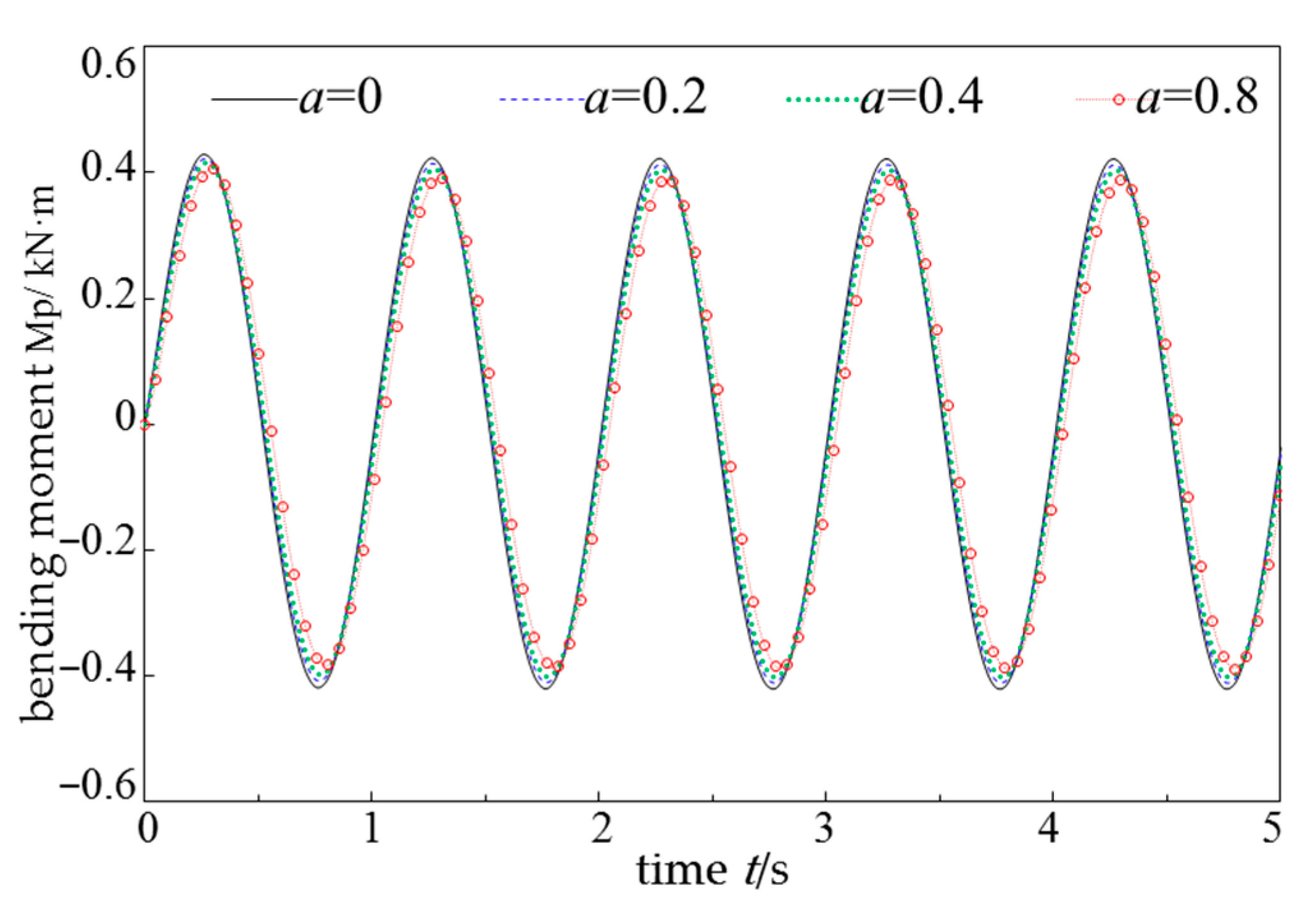
- The stronger the rheological properties of the soil, the smaller the displacement amplitude of the pile foundation, and the higher the load frequency, the greater the decrease in displacement amplitude. The positive bending moment of the pile decreases with the increase in soil rheological properties, while the negative bending moment increases accordingly.
- (3)
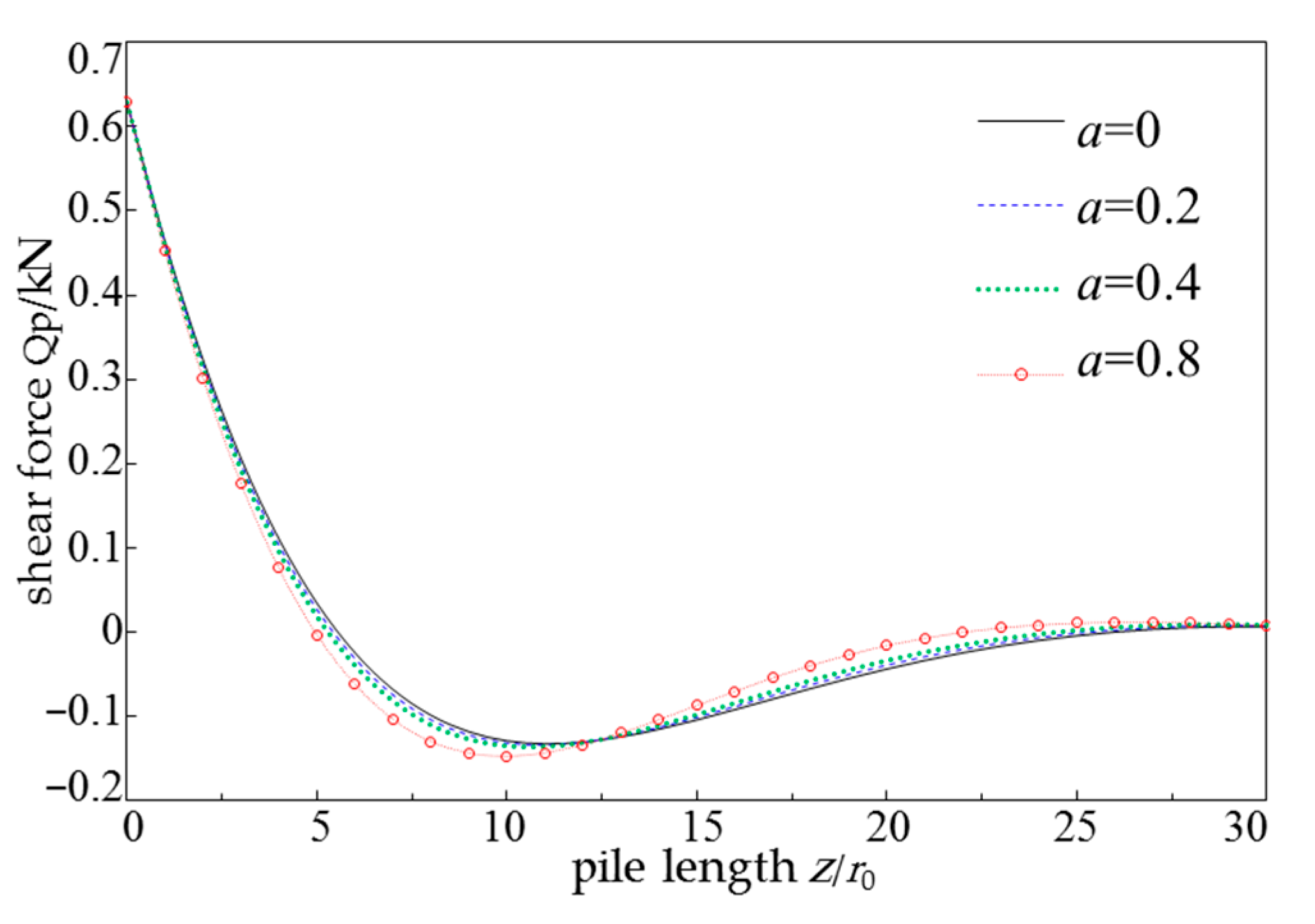
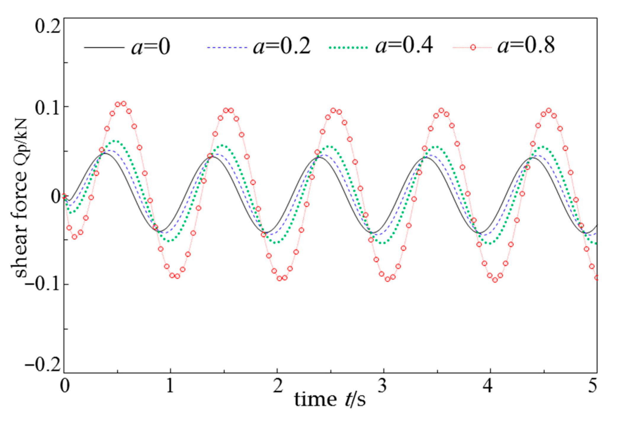
- The shear force at the top of the pile is not affected by the rheological properties of the soil, but both the positive and negative shear forces of the pile body significantly increase with the enhancement of the rheological properties of the soil. Therefore, when designing pile foundations in saturated clay, it is necessary to appropriately increase the pile diameter or increase the reinforcement to meet the shear performance.
Author Contributions
Funding
Institutional Review Board Statement
Informed Consent Statement
Data Availability Statement
Conflicts of Interest
Appendix A
References
- Biot, M.A. Theory of propagation of elastic waves in a fluid-saturated porous solid. II.Higher frequency range. J. Acoust. Soc. Am. 1956, 28, 179–191. [Google Scholar] [CrossRef]
- Dobry, R.; Gazetas, G. Simple method for dynamic stiffness and damping of floating pile groups. Geotechnique 1988, 38, 557–574. [Google Scholar] [CrossRef]
- Kaynia, A.M.; Kausel, E. Dynamics of piles and pile groups in layered soil media. Soil. Dyn. Earthq. Eng. 1991, 10, 386–401. [Google Scholar] [CrossRef]
- George, M.; George, G. Lateral vibration and internal forces of grouped piles in layered soil. J. Geotech. Geoenviron. Eng. 1999, 125, 16–25. [Google Scholar]
- Huang, S.; Chen, Y.; Zou, C. Train-induced environmental vibrations by considering different building foundations along curved track. Transp. Geotech. 2022, 35, 100785. [Google Scholar] [CrossRef]
- Rahmani, A.; Pak, A. Dynamic behavior of pile foundations under cyclic loading in liquefiable soils. Comput. Geotech. 2012, 40, 114–126. [Google Scholar] [CrossRef]
- Zarzalejos, J.M.; Aznárez, J.J.; Padrón, L.A.; Maeso, O. Influences of type of wave and angle of incidence on seismic bending moments in pile foundations. Earthq. Eng. Struct. Dyn. 2014, 43, 41–59. [Google Scholar] [CrossRef]
- Van Nguyen, Q.; Fatahi, B.; Hokmabadi, A.S. Influence of Size and Load-Bearing Mechanism of Piles on Seismic Performance of Buildings Considering Soil–Pile–Structure Interaction. Int. J. Geomech. 2017, 17, 0401700. [Google Scholar] [CrossRef]
- Chatterjee, K.; Choudhury, D.; Rao, V.D.; Poulos, H.G. Seismic response of single piles in liquefiable soil considering P-delta effect. Bull. Earthq. Eng. 2019, 17, 2935–2961. [Google Scholar] [CrossRef]
- Asker, K.; Fouad, M.T.; Bahr, M.; El-Attar, A. Numerical analysis of reducing tunneling effect on viaduct piles foundation by jet grouted wall. Min. Miner. Depos. 2021, 15, 75–86. [Google Scholar] [CrossRef]
- Jin, B.; Liu, H. Horizontal vibrations of a disk on a poroelastic half-space. Soil Dyn. Earthq. Eng. 2000, 19, 269–275. [Google Scholar] [CrossRef]
- Liu, Y.; Wang, X.; Zhang, M. Lateral Vibration of Pile Groups Partially Embedded in Layered Saturated Soils. Int. J. Geomech. 2014, 15, 04014063. [Google Scholar] [CrossRef]
- Zhang, S.; Cui, C.; Yang, G. Vertical dynamic impedance of pile groups partially embedded in multilayered, transversely isotropic, saturated soils. Soil Dyn. Earthq. Eng. 2019, 117, 106–115. [Google Scholar] [CrossRef]
- Liang, Z.; Cui, C.; Xu, C.; Zhang, P.; Wang, K. A close-formed solution for the horizontal vibration of a pipe pile in saturated soils considering the radial heterogeneity effect. Comput. Geotech. 2023, 158, 105379. [Google Scholar] [CrossRef]
- Liu, X.; El Naggar, M.H.; Wang, K.; Tu, Y.; Qiu, X. Simplified model of defective pile-soil interaction considering three-dimensional effect and application to integrity testing. Comput. Geotech. 2021, 132, 103986. [Google Scholar] [CrossRef]
- Hu, A.F.; Fu, P.; Xia, C.Q.; Xie, K.H. Lateral dynamic response of a partially embedded pile subjected to combined loads in saturated soil. Mar. Georesources Geotechnol. 2017, 35, 788–798. [Google Scholar] [CrossRef]
- Zou, X.; Yang, Z.; Wu, W. Horizontal dynamic response of partially embedded single pile in unsaturated soil under combined loads. Soil Dyn. Earthq. Eng. 2023, 165, 107672. [Google Scholar] [CrossRef]
- Cui, C.; Liang, Z.; Xu, C.; Xin, Y.; Wang, B. Analytical solution for horizontal vibration of end-bearing single pile in radially heterogeneous saturated soil. Appl. Math. Model. 2023, 116, 65–83. [Google Scholar] [CrossRef]
- Xu, C.; Dou, P.; Du, X.; El Naggar, M.H.; Miyajima, M.; Chen, S. Large shaking table tests of pile-supported structures in different ground conditions. Soil Dyn. Earthq. Eng. 2020, 139, 106307. [Google Scholar] [CrossRef]
- Tan, T.K. One dimensional problems of consolidation and secondary time effcets. China Civil Engineering. 1958, 5, 1–10. [Google Scholar]
- Chen, Z.; Liu, H.X. Two dimensional problems of settlements of clay layers due to consolidation and secondary time effects. Chin. J. Theor. Appl. Mech. 1958, 2, 1–10. [Google Scholar]
- Kabbaj, M.; Tavenas, F.; Leroueil, S. In situ and laboratory stress-strain relationships. Géotechnique 1988, 38, 83–100. [Google Scholar] [CrossRef]
- Koeller, R.C. Applications of fractional calculus to the theory of viscoelasticity. J. Appl. Mech. 1984, 51, 299–307. [Google Scholar] [CrossRef]
- Mandelbort, B.B. The Fractal Geometry of Nature; WH Freeman: New York, NY, USA, 1982; Volume 1. [Google Scholar]
- Zhao, M.; Huang, Y.; Wang, P.; Xu, H.; Du, X. Analytical solution of water pile soil interaction under horizontal dynamic loads on piel head. Chin. J. Geotech. Eng. 2022, 44, 907–915. [Google Scholar]
- Crump, K.S. Numerical inversion of Laplace transforms using a Fourier series approximation. J. ACM 1976, 23, 89–96. [Google Scholar] [CrossRef]
- Lian, W.; Jianchang, Z.; Zuowei, W. Analytical study on ground vibration induced by moving vehicle. Chin. J. Theor. Appl. Mech. 2020, 52, 1509–1518. [Google Scholar]
- Zhu, H.H.; Zhang, Z.X.; Liao, S.M. Underground Structure; China Building Industry Press: Beijing, China, 2005. [Google Scholar]
- Chang, X.M.; Gao, F.; Lu, Z.T.; Long, L.L.; Zhang, J.; Geng, X. A study on lateral transient vibration of large diameter piles considering pile-soil interaction. Soil Dyn. Earthq. Eng. 2016, 90, 211–220. [Google Scholar] [CrossRef]
- Yin, J.H. Non-linear creep of soils in oedometer tests. Géotechnique 1999, 49, 699–707. [Google Scholar] [CrossRef]
- Han, H.; Cui, W.; Li, Y. Dynamic characteristics of pile foundation under horizontal vibration load. J. Vib. Shock 2015, 34, 127–132. [Google Scholar]
- Tang, M.X.; Da, L. Vibration Theory and Applications; Tsinghua University Press: Beijing, China, 2005. [Google Scholar]


| H/m | r0/m | Ep/GPa | ρp/(kg·m−3) | Es/MPa | v |
|---|---|---|---|---|---|
| 20 | 0.5 | 28.5 | 2400 | 5.5 | 0.25 |
| n | kf/(m·s−1) | ρs/(kg·m−3) | ρf/(kg·m−3) | α | M/GPa |
| 0.4 | 2.0 × 10⁻⁷ | 2700 | 1000 | 1.0 | 4.9 |
Disclaimer/Publisher’s Note: The statements, opinions and data contained in all publications are solely those of the individual author(s) and contributor(s) and not of MDPI and/or the editor(s). MDPI and/or the editor(s) disclaim responsibility for any injury to people or property resulting from any ideas, methods, instructions or products referred to in the content. |
© 2024 by the authors. Licensee MDPI, Basel, Switzerland. This article is an open access article distributed under the terms and conditions of the Creative Commons Attribution (CC BY) license (https://creativecommons.org/licenses/by/4.0/).
Share and Cite
Ren, X.; Wang, L.-a. Study on the Time Domain Semi Analytical Method for Horizontal Vibration of Pile in Saturated Clay. Appl. Sci. 2024, 14, 778. https://doi.org/10.3390/app14020778
Ren X, Wang L-a. Study on the Time Domain Semi Analytical Method for Horizontal Vibration of Pile in Saturated Clay. Applied Sciences. 2024; 14(2):778. https://doi.org/10.3390/app14020778
Chicago/Turabian StyleRen, Xin, and Li-an Wang. 2024. "Study on the Time Domain Semi Analytical Method for Horizontal Vibration of Pile in Saturated Clay" Applied Sciences 14, no. 2: 778. https://doi.org/10.3390/app14020778