Simultaneous Identification of Multiple Parameters in Wireless Power Transfer Systems Using Primary Variable Capacitors

Featured Application

The methodology proposed in this article can be employed to improve the capability of the transmitting end of a WPT system to identify and adapt to parameter variations.

Abstract

This paper proposes a novel approach to simultaneously identifying multiple critical parameters in a wireless power transfer (WPT) system, such as the resonant frequency, mutual inductance, and load resistance, solely from the primary side. The key is to adopt a primary-side-switch-controlled capacitor (SCC) to ensure that the imaginary part of the input impedance is only caused by the secondary-side reflected impedance at three predesigned frequencies. The DSP controller then samples and processes the primary voltage and current using a gradient descent algorithm to derive the above parameters. After the identification, the SCC adjusts its equivalent capacitance based on the secondary-side practical resonant frequency to ensure a zero-phase angle (ZPA), thereby significantly improving the compatibility of the WPT system with unknown receivers. Compared to the previous frequency-sweeping method, the proposed approach is simpler and more suitable for deployment on the controller. Finally, experimental results demonstrate that the identification error of mutual inductance and resonant frequency are within 7.5% and 2.68%, respectively.

1. Introduction

Wireless power transfer (WPT), as a groundbreaking technology, enables more convenient access to energy in a cordless way. In recent years, WPT has garnered significant interest from researchers and has become increasingly popular in a variety of applications, such as in electric vehicles [1], induction heating [2], lighting [3], and medical implants [4]. In general, wireless power transfer (WPT) systems utilize different compensation topologies to minimize the reactive power produced by the coil inductance. The series–series (SS) topology is commonly that preferred out of various compensation networks because it does not rely on mutual inductance or load resistance [5]. To effectively implement crucial controls in a WPT system, such as maximum energy efficiency tracking (MEET) [6,7] and impedance matching across a broad load range [8,9], it is essential to have precise knowledge of critical parameters like the resonant frequency, mutual inductance, and load resistance. Whether it is WPT for electronic devices that should comply with the Qi standard (87 kHz~205 kHz) [10] or WPT for electric vehicles that should meet the SAEJ2954 standard (79 kHz~90 kHz) [11], the resonant frequency will vary across a wide range. Therefore, it is crucial to know the actual resonant frequency of the receiver before running the primary inverter at the corresponding resonant frequency. Hence, the critical parameters of mutual inductance, load resistance, and resonant frequency should be accurately identified before operating the WPT system, as minor deviations in these parameters can result in a significant decrease in performance.

Numerous researchers have investigated parameter identification from various perspectives and gained fruitful results. For instance, Wang et al. introduced a technique for detecting load resistance by applying an excitation on the inverter side; then, the load resistance can be calculated based on the time constant of system discharge or the envelope of current decay [12]. While this method is limited to a purely resistive load (e.g., heaters) and a fixed mutual inductance, Lin et al. proposed a genetic algorithm (GA) to search for the mutual inductance (actually replaced by coil spacing) and the resonant capacitance of multiple-stage coils by using frequency sweeping in the range of 450 kHz to 580 kHz [13]. Similarly, Yin et al. presented a front-end parameter monitoring method of mutual inductance and load resistance for two receivers [14]. On the other hand, Yang et al. addressed the scenario of multiple receivers using two-layer adaptive differential evolution (ADE) [15]. Gong et al. presented the parameter identification based on the LCC topology of the WPT system [16]. However, the aforementioned methods that involve wide frequency sweeping are computationally expensive and may only be feasible on a high-end computer rather than on an industrial controller such as the digital signal processor (DSP).

To observe the mutual inductance and load resistance during the steady-state operation of a WPT system, Liu et al. proposed a new method by assuming that the parameters of the secondary-side resonant tank are known, in which the precise waveform of the input voltage is required to obtain the amplitudes of the fundamental and third harmonics as well as the harmonics of the current [17]. In addition, it is noted in [18] that continuous frequency modulation of the inverter is necessary to achieve in-phase input voltage and current. However, this method may result in prolonged observation times, system instability, and load variations. Alternatively, Yang et al. and Zeng et al. achieved mutual inductance identification within the millisecond range using fast frequency sweeping and hardware phase detection techniques without information on the transmitter and receiver resonators [19,20].

In recent years, machine learning-based parameter identification methods have attracted attention. He et al. utilized artificial neural networks to identify mutual inductance [21], while Zhang et al. adopted support vector regression (SVR) to identify mutual inductance and load resistance [22]. However, their data collection and testing are based on a single experimental setup, limiting the ability to demonstrate model transferability. Additionally, these methods increase data collection costs and pose challenges for the adaptation of WPT systems to multiple coils. It is worth noting that most identification methods identify a single parameter or two parameters based on the known parameters on both the primary and secondary sides. Traditional observation approaches suffer from several limitations, such as high-frequency sweeping, slow observation speed, and the inability to observe actual the secondary side aresonant frequency.

This paper presents a new method to address these challenges by simultaneously identifying three critical parameters in a WPT system, namely, load resistance, mutual inductance, and actual resonant frequency. The proposed method simplifies the identification process by only requiring input current and voltage values at three predetermined operating frequencies. Observations can be made using the gradient descent algorithm and can be quickly executed on a DSP. Moreover, the primary-side variable capacitor, comprising a standard capacitor and a switch-controlled capacitor (SCC) connected in series, can adjust the equivalent capacitance to compatibly accommodate receivers even though their resonant frequencies are unknown or have drifted. Section 2 will illustrate the parameter identification model. In Section 3, the experimental prototype will be constructed to validate the effectiveness of the proposed method. Finally, a conclusion will be drawn in Section 4.

2. System Design and Analysis

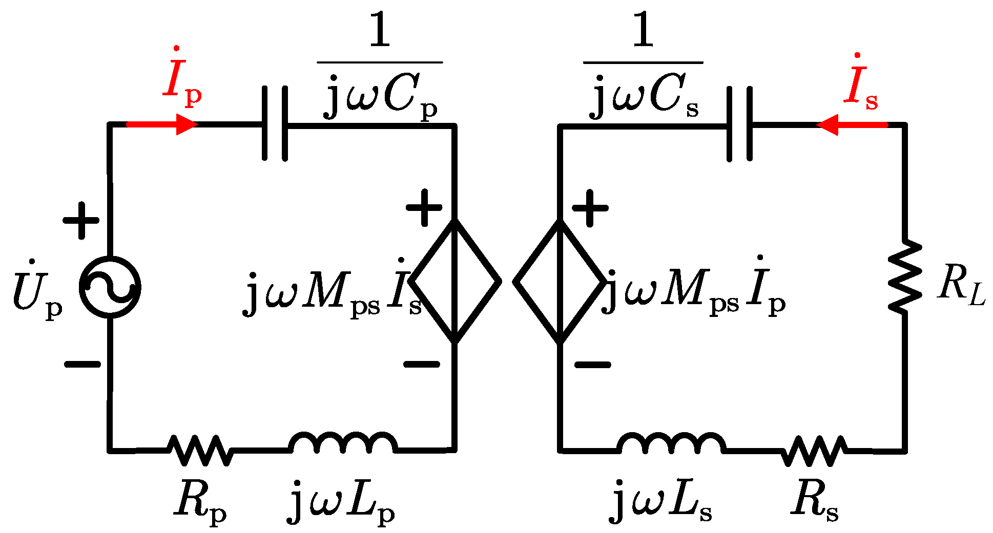
2.1. Circuit Model Analysis

Figure 1 shows the circuit model of a two-coil SS-compensated WPT system in which L_p (L_s) and M_ps are primary (secondary) self-inductance and mutual inductance, respectively. R_p stands for the equivalent resistance composed of the coil resistance and equivalent series resistance (ESR) of the compensation capacitor C_p. The operating angular frequency ω is determined by the voltage-fed power source u_p, and the natural resonant angular frequency of the WPT system is given by (1) and (2).

$${\omega }_p^2{L}_p{C}_p=1$$

(1)

$${\omega }_s^2{L}_s{C}_s=1$$

(2)

$$\left(R_p+\mathrm{j}{X}_p\right)\dot{I_p}+\mathrm{j}\omega M_{ps}\dot{I_s}=\dot{U_p}$$

(3)

$$\mathrm{j}\omega M_{ps}\dot{I_p}+\left(R_s+R_L+\mathrm{j}{X}_s\right)\dot{I_s}=0$$

(4)

After implementing KVL on both sides, the system can be expressed with (3) and (4), where $\dot{U_p}$, $\dot{I_p}$  and $\dot{I_s}$  are phasors of fundamental input ac voltage, with current passing through primary and secondary coils. X_p and X_s refer to the reactance of resonators on both sides, respectively.

If the system-operating-angular frequency is set to ω_p, then X_p will be eliminated. The relation between $\dot{U_p}$  and $\dot{I_p}$  is given in (5), where the second term on the right hand of the equation is the reflected impedance brought by the secondary side. It should be noted that (5) also expressed the value of input impedance Z_in, whose real and imaginary parts are provided in (6) and (7). The value of R_s is omitted because it is usually negligible compared to R_L.

$$\frac{\dot{U_p}}{\dot{I_p}}=R_p+\frac{{\omega }_p^2{M}_{ps}^2}{R_L+R_s+\mathrm{j}{X}_s}$$

(5)

$$\mathrm{R}\mathrm{e}\left[Z_{in}\right]=R_p+\frac{{\omega }_p^2{M}_{ps}^2{R}_L}{R_L^2+X_s^2}$$

(6)

$$\mathrm{I}\mathrm{m}\left[Z_{in}\right]=-\frac{{\omega }_p^2{M}_{ps}^2{X}_s}{R_L^2+X_s^2}$$

(7)

$$\left\{\begin{array}{c}Re\left[Z_{in}\right]=f(R_L,M_{ps},L_s,C_s)\\ Im\left[Z_{in}\right]=g(R_L,M_{ps},L_s,C_s)\end{array}\right.$$

(8)

Normally, the primary-side ω_p, R_p and $\dot{U_p}$  are known parameters, and then the input impedance Z_in can be expressed as a function with M_ps, L_s, C_s, and R_L being variables, as shown in (8). In that case, as long as the root-mean-square (RMS) value of $\dot{I_p}$  and its phase relative to the input voltage under different ω_p are obtained, multiple equations of Formula (8) can be deduced. Since the equation cannot be explicitly expressed, it is transformed into the solution of an optimization problem.

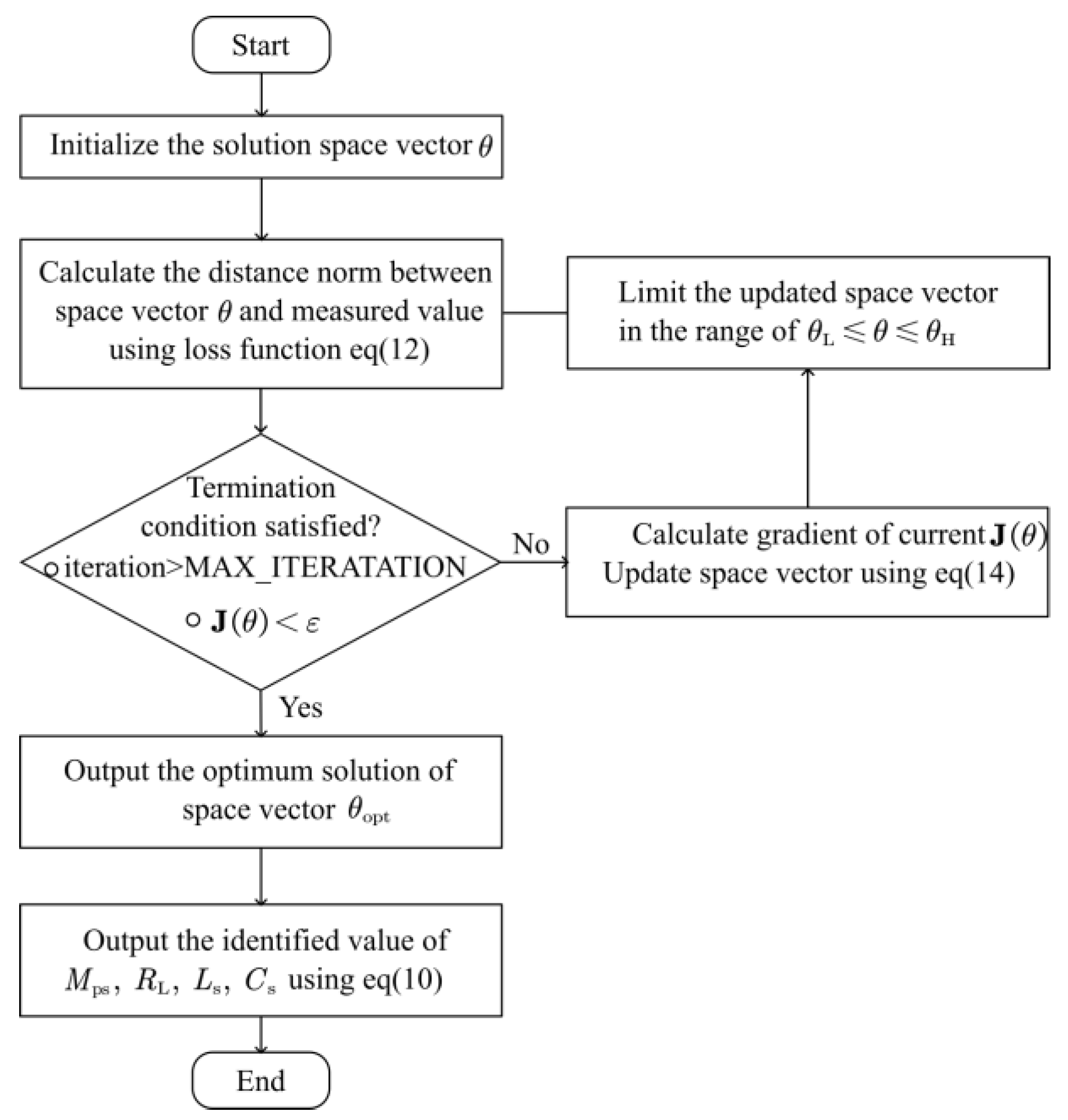
2.2. Gradient Descent for Parameter Identification

Gradient descent is an iterative optimization algorithm that minimizes (or maximizes) a function, typically a cost or loss function. The fundamental concept underlying the gradient descent algorithm is to iteratively modify the model parameters or function variables in a manner that aligns with the steepest descent of the objective function’s gradient (or slope) concerning these variables. The gradient signifies the direction in which the function exhibits the most rapid ascent. Hence, by proceeding in the opposite direction, the objective is to effectively approach the function’s minimum value, thereby facilitating the optimization process.

$$\theta =[X_{m1},R_L,X_{L1},X_{c1}]$$

(9)

$$\left\{\begin{array}{c}{X}_{m1}={\omega }_{p1}{M}_{ps}\\ X_{L1}={\omega }_{p1}{L}_s\\ X_{c1}=1/\left({\omega }_{p1}{C}_s\right)\end{array}\right.$$

(10)

$${\omega }_{pi}^2{L}_p{C}_{pi}=1 (i=\mathrm{1,2},3)$$

(11)

Firstly, a parameter vector θ is defined in (9), where X_m1, X_L1, and X_C1 are the reactance of M_ps, L_s, and Cs, respectively, when the operating angular frequency of the system is ω_p1, which is derived by (10) and (11). Different values of ω_p are achieved by alternating the capacitance value, which will be discussed in the next section. The three primary resonant frequencies were chosen because this is the minimum amount of data required to identify mutual inductance, secondary resonant frequencies, and load resistance simultaneously. It is important to note that using the reactance value of these passive elements instead of their inductance or capacitance can improve the convergence of computation. This is particularly crucial if the algorithm is to be deployed in DSPs or other embedded devices.

$$\mathbf{J}\left(\theta \right)={\sum }_{i=1}^3[{\left(\mathrm{R}\mathrm{e}\left[Z_{\theta }\right]-\frac{U_p}{I_{pi}}\cdot cos{\phi }_i\right)}^2+{\left(\mathrm{I}\mathrm{m}\left[Z_{\theta }\right]-\frac{U_p}{I_{pi}}\cdot sin{\phi }_i\right)}^2]$$

(12)

(The next step is to formulate the loss function, which is given in (12). The loss function describes the magnitude of the distance norm, which is the difference between the measured input impedance Z_in and the calculated input impedance Z_θ in the solution space. Since the secondary side is not necessarily in a resonant state, the reflected impedance will have an imaginary part on the primary side. $I_{pi}$  is the RMS values of $\dot{I_p}$  and φ_i is the phase difference between $\dot{U_p}$  and $\dot{I_p}$  when the operating angular frequency of the system is at ω_pi.

$$\left\{\begin{array}{c}{\theta }_L<\theta <{\theta }_H\\ {\theta }_L=[{\omega }_{p1}{M}_{psmin},R_{Lmin},{\omega }_{p1}{L}_{smin},1/\left({\omega }_{p1}{C}_{smax}\right)\\ {\theta }_H=[{\omega }_{p1}{M}_{psmax},R_{Lmax},{\omega }_{p1}{L}_{smax},1/\left({\omega }_{p1}{C}_{smin}\right)\end{array}\right.$$

(13)

$${\theta }_k={\theta }_{k-1}-\alpha \cdot \frac{\mathsf{\Delta }\mathbf{J}\left({\theta }_{k-1}+\mathbf{h}\right)-\mathsf{\Delta }\mathbf{J}\left({\theta }_{k-1}-\mathbf{h}\right)}{2\mathbf{h}}$$

(14)

Accordingly, the solution space that is the value space of θ can be given. And the size of the space determines the range of parameter identification of the system, which is described by (13). After initializing θ, the learning rate α, the iteration step h, and the precision parameter ε, the gradient descent algorithm will output the identified values of M_ps, R_L, and parameters of the secondary resonator by updating the space vector with (14), in which k represents the kth iteration until the termination condition is satisfied. Termination occurs when the iteration process exceeds its set maximum value or the computation converges. The complete gradient descent algorithm for parameter identification is shown in Figure 2.

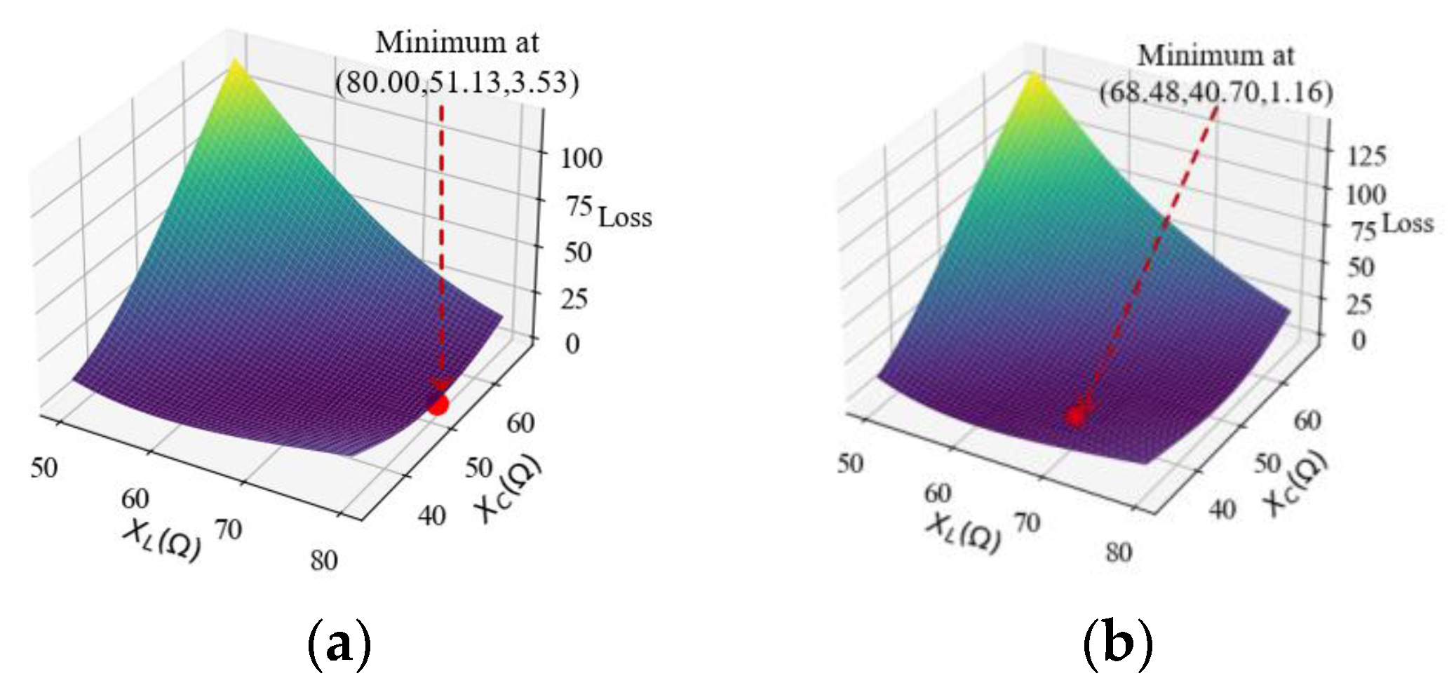
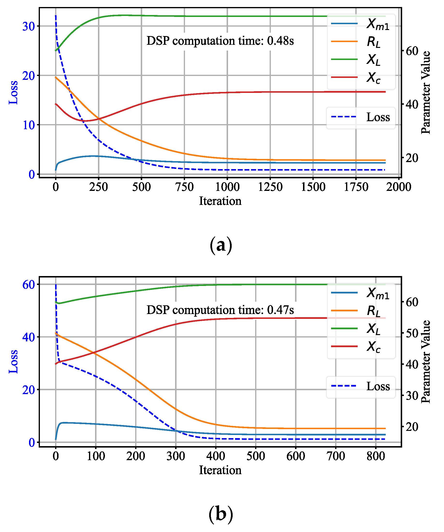
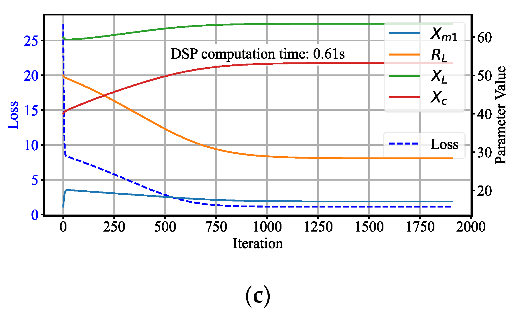
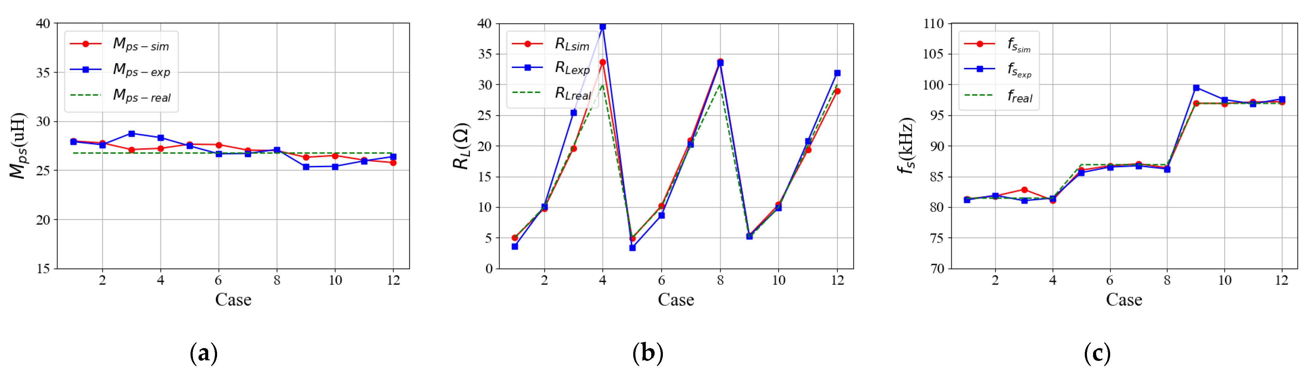
2.3. Verification via Simulation

Figure 3 illustrates the system configuration for the proposed method, namely the simultaneous identification of multiple parameters in WPT systems. The signal generator works together with the power amplifier as a high-frequency voltage source u_p. The primary variable capacitor, namely the SCC, consists of two constant capacitors: one is connected with a relay switch S_r in parallel and another is connected with two MOSFETs switches in parallel. Thus, the SCC can operate in three modes:

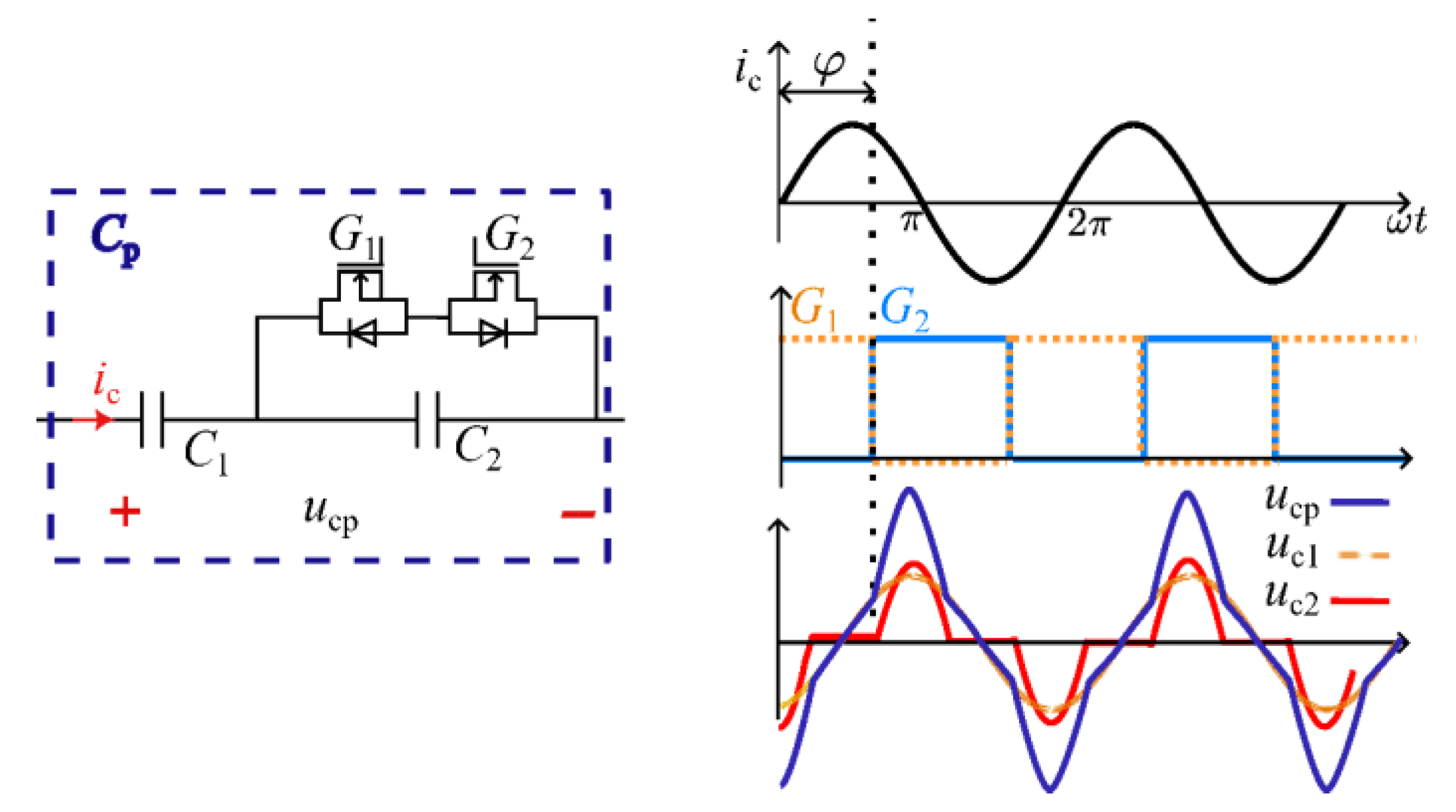
• When the relay S_r is open, and both MOSFETs paralleled with C₂ are conducting, the equivalent capacitance overall is C₁.
• When the relay S_r is closed, and both MOSFETs paralleled with C₂ are turned off, the equivalent capacitance overall is C₂.
• When the relay S_r is open, C₂ and the two MOSFETs paralleled to form an SCC, which can achieve continuously adjustable capacitance from C₁ in series with C₂ to C₁.

The critical parameters in this paper are listed in

Table 1. Parameters of the proposed WPT system.

Item	Symbol	Value
Input voltage RMS	Up	7.07 V
Primary-side capacitor 1	C1	44 nF
Primary-side capacitor 2	C2	22 nF
Secondary-side capacitor	Cs	26.7, 33.2, 37.8 nF
ESR of transmitter	Rp	0.4 Ω
Self-inductance of transmitter	Lp	103 μH
ESR of receiver	Rs	0.4 Ω
Self-inductance of receiver	Ls	101 μH
Mutual inductance	Mps	26.7 μH
Load resistance	RL	5, 10, 20, and 30 Ω
Primary-side resonant frequency 1,2,3	fp1,2,3	105.73, 74.76, and 129.49 kHz
Secondary-side resonant frequency	fs	81.45, 86.9, and 96.9 kHz
Lower bound of space vector	θL	[5, 2, 50, and 33.3] Ohm
Upper bound of space vector	θH	[30, 50, 80, and 66.6] Ohm

. The variation of primary equivalent capacitance corresponds to the change of primary resonant frequency from 75 to 130 kHz, which can cover the frequency range required in the SAEJ2954 standard. In this paper, three predetermined frequencies, f_p1,2,3 of 74.76, 105.73, and 129.49 kHz, are utilized to achieve the parameter identification. The values of such frequencies are designated to accommodate the resonant frequency range (75 kHz~130 kHz) on the secondary side. Moreover, regardless of the variation of the parameters to be identified, the above three frequencies are used in each identification case, the range of which is defined by the lower and upper bounds of the space vector. It should be noted that the proposed system can easily identify and accommodate unknown receivers as long as their actual resonant frequencies are within the aforementioned range. To identify unknown receivers with different resonant frequencies and load conditions, the secondary capacitance C_s and load resistance R_L were intentionally adjusted from 22 to 45 nF and from 2 to 50 Ω in solution space, respectively. For simplifying the verification, the C_s are deliberately set to 26.7, 33.2, and 37.8 nF when the secondary coil inductance L_s is constant at 101 μH, which in turn corresponds to the f_s of 81.45, 86.9, and 96.9 kHz, respectively. In any case, mutual inductance varies from 10 to 50 μH in solution space.

As shown in Figure 4, twelve cases of simulation were conducted with variations of secondary resonant frequency f_s and load resistance R_L. Cases i, i + 1, i + 2, and i + 3 (i = 1,5,9) share the same f_s value, while Cases j, j + 4, j + 8 (j = 1, 2, 3, 4) share the value of R_L that is shown in Figure 4b. The dotted line in the figure is the set value in the simulation. By comparing the identified values of M_ps, R_L, and fs derived from (12) with the set value, it can be seen that the parameter identification basically functions as predicted but is not precise enough. The maximum identified errors of mutual inductance, load resistance, and secondary resonant frequency are about 2.6 μH, 4.78 Ω, and 5.24 kHz, respectively. To further explore how to increase the accuracy of the algorithm, the worst case (Case 4), which shows the maximum identified error in all parameters, is studied. Its loss surface is demonstrated in Figure 5a to see the location of the optimum point delivered by the algorithm. The loss surface is flat near the optimum point, which means that the algorithm is not able to distinguish the differences in the dark-colored area. Also, the solution given by the current algorithm is at the edge of the loss surface, which means that it is not the solution that we predicted.

To solve this issue, we modified the loss function by using Equation (15), where k represents the weight assigned to the deviation of the real and imaginary parts. By counting the errors between the real part and the imaginary part during the convergence process, we found that the real part error is more significant. Increasing the k value can make the optimization process pay more attention to this part of the error and improve the identification accuracy. Thus, in future experiments, the imaginary part will only have 1/10th of the weight in the loss function.

$$\mathbf{J}\left(\theta \right)=\sum _{i=1}^3[{k\cdot \left(\mathrm{R}\mathrm{e}\left[Z_{\theta }\right]-\frac{U_p}{I_{pi}}\cdot cos{\phi }_i\right)}^2+\left(1-k\right)\cdot {\left(\mathrm{I}\mathrm{m}\left[Z_{\theta }\right]-\frac{U_p}{I_{pi}}\cdot sin{\phi }_i\right)}^2]$$

(15)

In Figure 4, the blue curves in all sub-graphs present the results of the simulation after implementing the new loss function from (15). The accuracy has greatly improved, with the maximum identified errors for mutual inductance, load resistance, and secondary resonant frequency being 1.25 μH, 3.8 Ω, and 1.41 kHz, respectively. The optimized loss function, as shown in Figure 5b, has a more defined loss surface, which aids in distinguishing the desired solution from the surrounding points during gradient descent. As a result, the solution obtained will lie within the contour of the surface, rather than on the edge of the surface as before.

To further illustrate the difference between the two loss functions, a box-plot is presented in Figure 6 that shows the deviation between the identified value and the set value. Utilizing the original loss Function (12) results in a smaller estimated mean and more dispersed data. On the other hand, the new loss Function (15) allows for smaller errors and more concentrated data in the identified parameters.

The process of convergence is shown in Figure 7, which gives the process of updating the parameters of space vector as well as minimizing the loss function. Although these plots are derived by calculation on PC, the ultimate results on different platforms are the same. It can be seen that after about 2000 and 800 iterations, the space vector with four variables gradually becomes constant in calculations shown in Figure 7a,b, which are simulated with the same load resistance of 20 Ω while their secondary-side resonant frequencies are not the same. On the contrary, the calculations shown in Figure 7b,c share the same f_s with different load conditions. Convergence in Figure 7c takes almost the same number of iteration steps as in Figure 7a. The algorithm is then deployed on TMS32028335 to test its real-time performance. According to DSP testing, the algorithm requires approximately 6,988,139~91,767,151 clock cycles to complete, taking about 0.47~0.61 s. Compared to the previous GA, ADE, and double-layer ADE algorithms, which required approximately 30 s for computation on a computer [15], our algorithm increases the number of identifiable parameters while significantly improving real-time performance. This enhancement also facilitates its feasibility for deployment on actual embedded platforms.

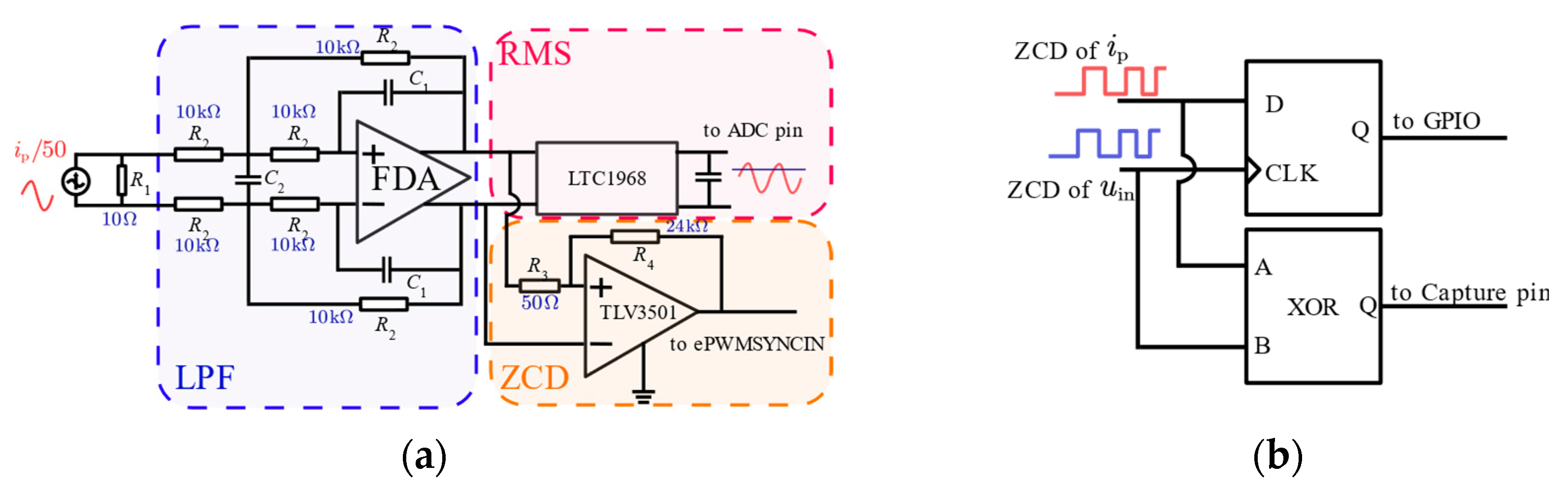
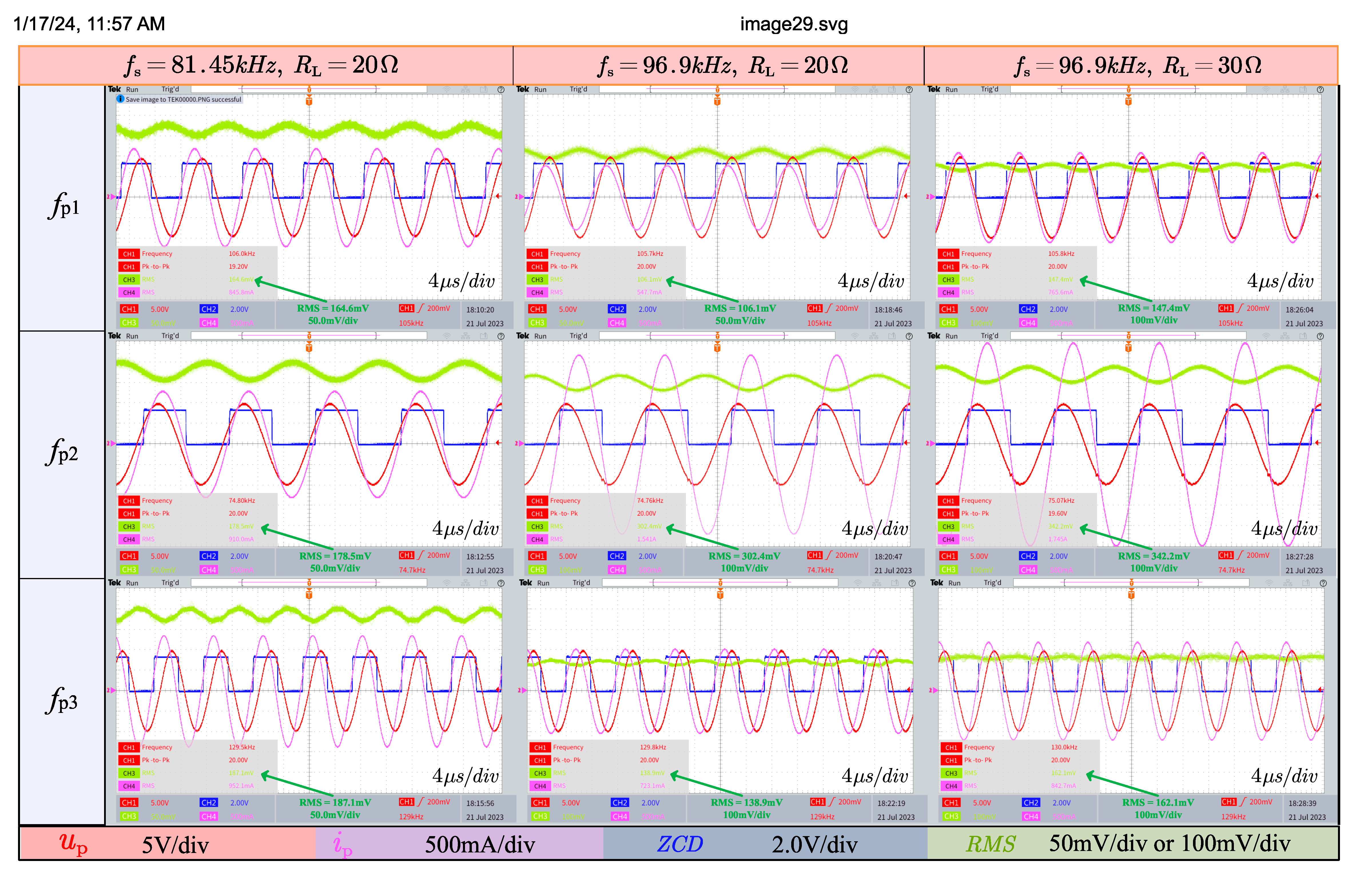
3. Experimental Implementation

As shown in Figure 8, experiments were conducted to verify the feasibility of the proposed parameter identification method and the system’s multi-frequency operating capability. The input voltage source for the power amplifier and the voltage reference signal for the signal processing board were provided by the function generator DG822. The TMS32028335 was chosen as the DSP to implement the gradient descent algorithm. Different resonant frequencies on the secondary side were achieved by adjusting the compensation capacitor C_s, while load conditions were emulated by changing the number of resistors connected to the circuit. To ensure that the system achieve a resonant state on both the primary and secondary sides, the 650 V MOEFET IMBG65R072M1H was selected to act as the power switch in SCC.

As shown in Figure 9a, primary-side current i_p is converted to voltage signal by a current transformer that set current decay at 1/50 and by a high precision resistor. A second order Butterworth LPF is implemented to filter out interference signals above 800 kHz. It should be noted that this filter will contribute about 0.3 µs delay to the signal. Then, the filtered signal will be transformed to an RMS value using LTC1968 and to a zero-cross-detection (ZCD) signal by a high-speed comparator TLV3501. The ZCD signal of current will be fed into the phase detection circuit and the ePWMSYNCIN pin of DSP to generate a control signal of SCC. Phase detection in Figure 9b is realized by D flip-flop and Exclusive OR (XOR) gates, the former of which indicates whether the current is leading or lagging, with the ZCD of voltage being a reference. The XOR gate will produce a signal that contains information on the absolute phase difference.

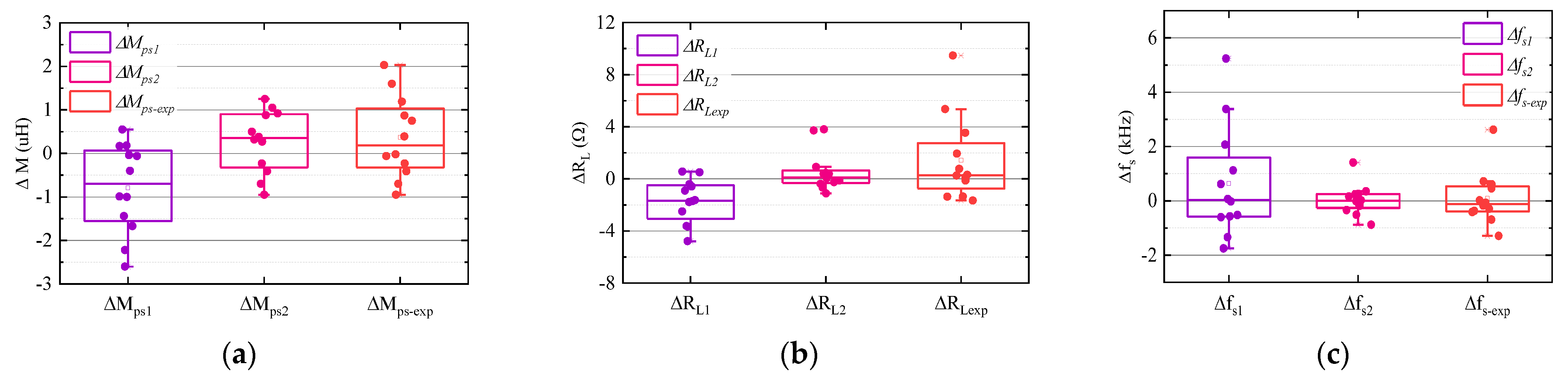
3.1. Parameter Identification

The procedure for performing parameter identification is as follows:

• Choose the output frequency of the function generator.
• Select the correct mode of C_p.
• Log the data of I_pi, φ_i.
• Perform the GD Algorithm.

Figure 10 shows the waveform of input voltage u_p, input current i_p, ZCD signal of i_p, and RMS output of the circuit during the parameter identification process. u_p is kept at 20 Vpp in all cases. It should be noted that the RMS output is 0.2 times the actual value, and it exhibits a certain degree of fluctuation, which means that digital filtering by DSP after ADC sampling is necessary. The ZCD signal has a time delay of 0.3 µs, which needs to be compensated for during the phase-difference calculation.

Figure 11 shows that the measured results are similar to the simulated results. When the load resistance is large, such as for Cases 4, 8, and 12, the identification errors of R_L and f_s are larger, and this trend is also observed in the simulation results. The maximum identification errors for mutual inductance, load resistance, and f_s are 2.03 μH, 9.47 Ω, and 2.62 kHz, respectively. Although the resistance-identification error in Case 4 is relatively large, the experimental results still prove the feasibility of the identification method.

3.2. Accommodation of Unknown Receivers

The concept of SCC was first proposed by Harada et al. in [23]; its structure and typical waveform are shown in Figure 12, in which φ is the control angle. The current flowing through SCC is taken as a reference. After capturing its ZCD signal, complementary PWM signals are sent to two MOSFETs set up in parallel with the capacitor. Since the SCC has the characteristics of continuously adjusting the equivalent capacitance, the WPT system can use SCC on the primary side to adjust the resonant frequency equivalently, which in turn can accommodate unknown receivers with different resonant frequencies.

$$C_{scc}=\frac{\pi C_1}{2\pi -2\phi +sin2\phi }$$

(16)

$${\omega }_s^2\left(\frac{1}{\frac{1}{C_1}+\frac{1}{C_{scc}}}\right)L_p$$

(17)

With a radian-format control angle φ, the SCC equivalent capacitance is given in (16). The calculation is based on the fundamental harmonic analysis (FHA) and the assumption that a sinusoidal current flows through the SCC. For detailed derivation, please refer to [23]. Theoretically, the SCC in this paper can adjust its capacitance from C₂ to infinity. However, φ ranges from π/2 to π, which means that when the value of the control angle is close to π, a slight difference will lead to a significant change in the equivalent capacitance, as shown in Figure 13a. Once the SCC is series-connected to C₁, not only does the overall capacitor voltage u_cp become more sinusoidal, as shown in Figure 12, but it also creates a more linear relationship between the control angle and the equivalent capacitance, as presented in Figure 13b. This configuration enables the transmitter to operate in the ZPA state with receivers that have different resonant frequencies by calculating the corresponding value of C_scc by (17) and obtaining the control angle via a look-up table. To show the accommodation capability of the receivers with different resonant frequencies, three identification cases with the actual resonant frequencies of the receivers, 81.45 kHz, 86.9 kHz, and 96.9 kHz, respectively, are conducted as illustrated in Figure 14. The input voltage and load resistance are kept at 90 Vpp and 30 Ω, respectively. It can be seen that the u_p and i_p are in phase and the system efficiency can be maintained above 80% for all cases.

4. Conclusions

This paper presents a novel approach to identifying multiple critical parameters of a WPT system from the primary side, including the resonant frequency, mutual inductance, and load resistance. The approach utilizes an SCC to ensure that the imaginary part of the input impedance is solely caused by the secondary-side reflected impedance at three selected frequencies. The parameters are derived using a gradient descent algorithm, and the SCC adjusts its equivalent capacitance to achieve the primary ZPA based on the secondary different resonant frequencies, which can significantly improve the compatibility of the WPT system with unknown receivers. The experimental results show that the identification error of mutual inductance and resonant frequency are within 7.5% and 2.68%, respectively. Compared to the previous frequency-sweeping method, this approach is simpler and more suitable for deployment on embedded devices.

References

1. Zhang, Z.; Pang, H.; Georgiadis, A.; Cecati, C. Wireless Power Transfer—An Overview. IEEE Trans. Ind. Electron. 2019, 66, 1044–1058. [Google Scholar] [CrossRef]
2. Han, W.; Chau, K.T.; Liu, W.; Tian, X.; Wang, H. A Dual-Resonant Topology-Reconfigurable Inverter for All-Metal Induction Heating. IEEE J. Emerg. Sel. Top. Power Electron. 2022, 10, 3818–3829. [Google Scholar] [CrossRef]
3. Han, W.; Chau, K.T.; Jiang, C.; Liu, W.; Lam, W.H. Design and Analysis of Wireless Direct-Drive High-Intensity Discharge Lamp. IEEE J. Emerg. Sel. Top. Power Electron. 2020, 8, 3558–3568. [Google Scholar] [CrossRef]
4. Haerinia, M.; Shadid, R. Wireless Power Transfer Approaches for Medical Implants: A Review. Signals 2020, 1, 209–229. [Google Scholar] [CrossRef]
5. Qu, X.; Jing, Y.; Han, H.; Wong, S.-C.; Tse, C.K. Higher Order Compensation for Inductive-Power-Transfer Converters with Constant-Voltage or Constant-Current Output Combating Transformer Parameter Constraints. IEEE Trans. Power Electron. 2017, 32, 394–405. [Google Scholar] [CrossRef]
6. Zhong, W.X.; Hui, S.Y.R. Maximum Energy Efficiency Tracking for Wireless Power Transfer Systems. IEEE Trans. Power Electron. 2015, 30, 4025–4034. [Google Scholar] [CrossRef]
7. Dai, X.; Li, X.; Li, Y.; Hu, A.P. Maximum Efficiency Tracking for Wireless Power Transfer Systems with Dynamic Coupling Coefficient Estimation. IEEE Trans. Power Electron. 2018, 33, 5005–5015. [Google Scholar] [CrossRef]
8. Zhong, W.; Hui, S.Y. Reconfigurable Wireless Power Transfer Systems with High Energy Efficiency over Wide Load Range. IEEE Trans. Power Electron. 2018, 33, 6379–6390. [Google Scholar] [CrossRef]
9. Lim, Y.; Tang, H.; Lim, S.; Park, J. An Adaptive Impedance-Matching Network Based on a Novel Capacitor Matrix for Wireless Power Transfer. IEEE Trans. Power Electron. 2014, 29, 4403–4413. [Google Scholar] [CrossRef]
10. Qi Wireless Charging. Available online: https://www.wirelesspowerconsortium.com/standards/qi-wireless-charging/ (accessed on 15 January 2024).
11. J2954_202010; Wireless Power Transfer for Light-Duty Plug-in/Electric Vehicles and Alignment Methodology. SAE International: Warrendale, PA, USA, 2020. Available online: https://www.sae.org/standards/content/j2954_202010/ (accessed on 15 January 2024).
12. Wang, Z.-H.; Li, Y.-P.; Sun, Y.; Tang, C.-S.; Lv, X. Load Detection Model of Voltage-Fed Inductive Power Transfer System. IEEE Trans. Power Electron. 2013, 28, 5233–5243. [Google Scholar] [CrossRef]
13. Lin, D.; Yin, J.; Hui, S.Y.R. Parameter Identification of Wireless Power Transfer Systems Using Input Voltage and Current. In Proceedings of the 2014 IEEE Energy Conversion Congress and Exposition (ECCE), Pittsburgh, PA, USA, 14–18 September 2014. [Google Scholar]
14. Yin, J.; Lin, D.; Lee, C.K.; Parisini, T.; Hui, S.Y. Front-End Monitoring of Multiple Loads in Wireless Power Transfer Systems without Wireless Communication Systems. IEEE Trans. Power Electron. 2016, 31, 2510–2517. [Google Scholar] [CrossRef]
15. Yang, Y.; Tan, S.-C.; Hui, S.Y.R. Front-End Parameter Monitoring Method Based on Two-Layer Adaptive Differential Evolution for SS-Compensated Wireless Power Transfer Systems. IEEE Trans. Industr. Inform. 2019, 15, 6101–6113. [Google Scholar] [CrossRef]
16. Gong, W.; Xiao, J.; Wu, X.; Chen, S.; Wu, N. Research on Parameter Identification and Phase-Shifted Control of Magnetically Coupled Wireless Power Transfer System Based on Inductor–Capacitor–Capacitor Compensation Topology. Energy Rep. 2022, 8, 949–957. [Google Scholar] [CrossRef]
17. Liu, J.; Wang, G.; Xu, G.; Peng, J.; Jiang, H. A Parameter Identification Approach with Primary-Side Measurement for DC–DC Wireless-Power-Transfer Converters with Different Resonant Tank Topologies. IEEE Trans. Transp. Electrif. 2021, 7, 1219–1235. [Google Scholar] [CrossRef]
18. Su, Y.-G.; Zhang, H.-Y.; Wang, Z.-H.; Patrick Hu, A.; Chen, L.; Sun, Y. Steady-State Load Identification Method of Inductive Power Transfer System Based on Switching Capacitors. IEEE Trans. Power Electron. 2015, 30, 6349–6355. [Google Scholar] [CrossRef]
19. Yang, Y.; Tan, S.C.; Hui, S.Y.R. Fast Hardware Approach to Determining Mutual Coupling of Series–Series-Compensated Wireless Power Transfer Systems with Active Rectifiers. IEEE Trans. Power Electron. 2020, 35, 11026–11038. [Google Scholar] [CrossRef]
20. Zeng, J.; Chen, S.; Yang, Y.; Hui, S.Y.R. A Primary-Side Method for Ultrafast Determination of Mutual Coupling Coefficient in Milliseconds for Wireless Power Transfer Systems. IEEE Trans. Power Electron. 2022, 37, 15706–15716. [Google Scholar] [CrossRef]
21. He, L.; Zhao, S.; Wang, X.; Lee, C.-K. Artificial Neural Network-Based Parameter Identification Method for Wireless Power Transfer Systems. Electronics 2022, 11, 1415. [Google Scholar] [CrossRef]
22. Zhang, H.; Tan, P.-A.; Shangguan, X.; Zhang, X.; Liu, H. Machine Learning-Based Parameter Identification Method for Wireless Power Transfer Systems. J. Power Electron. 2022, 22, 1606–1616. [Google Scholar] [CrossRef]
23. Harada, K.; Gu, W.J.; Murata, K. Controlled Resonant Converters with Switching Frequency Fixed. In Proceedings of the 1987 IEEE Power Electronics Specialists Conference, Blacksburg, VA, USA, 21–26 June 1987; IEEE: Piscataway, NJ, USA, 1987. [Google Scholar]
Figure 1. Circuit model of SS-WPT system.
Applsci 14 00793 g001
Figure 2. Flowchart of gradient descent algorithm used for parameter identification.
Applsci 14 00793 g002
Figure 3. System configuration for parameter identification with multi-frequency operating capability.
Applsci 14 00793 g003
Figure 4. Identified parameters and set values (green dotted line) in simulation with loss functions in (12) (red curve) and in (15) (blue curve). (a) Identified Mps; (b) identified RL; and (c) identified fs.
Applsci 14 00793 g004
Figure 5. Loss surface with fixed RL and Mps in Case 4 (a) using loss Function (12) and (b) using loss Function (15). Colors indicate varying loss values.
Applsci 14 00793 g005
Figure 6. Deviation between the identified values and the set values in simulations and experiments. Simulation results of implementing loss functions in (12) (purple box−plot) and (15) (pink box−plot) and experimental results (orange boxplot) are compared. (a) Identified Mps, (b) identified RL; and (c) identified fs.
Applsci 14 00793 g006
Figure 7. Space-vector update process with different Rx parameters. (a) fs = 81.45 kHz, RL = 20 Ω. (b) fs = 96.9 kHz, RL = 20 Ω. (c) fs = 96.9 kHz, RL = 30 Ω.
Applsci 14 00793 g007aApplsci 14 00793 g007b
Figure 8. The experimental setup.
Applsci 14 00793 g008
Figure 9. Circuits on signal processing board; (a) current detection and (b) phase detection.
Applsci 14 00793 g009
Figure 10. Waveforms of input voltage up, input current ip, ZCD signal of ip and RMS output of the circuit during parameter identification process. Three cases are given, each with different fs and RL.
Applsci 14 00793 g010
Figure 11. Identified parameters and corresponding differences from set values (dotted line) in experiments; (a) identified Mps, (b) identified RL; and (c) identified fs.
Applsci 14 00793 g011
Figure 12. The SCC with a series-connected capacitor and typical waveform of SCC.
Applsci 14 00793 g012
Figure 13. Graph of equivalent capacitance as a function of control angle. (a) Equivalent capacitance of SCC; and (b) equivalent capacitance of SCC connected with C1.
Applsci 14 00793 g013
Figure 14. Using SCC to realize ZPA at different operating frequencies.
Applsci 14 00793 g014