


Automated Think-Aloud Protocol for Identifying Students with Reading Comprehension Impairment Using Sentence Embedding


Abstract
1. Introduction
1.1. Reading Comprehension Impairment
1.2. Think-Aloud Protocol
1.3. Contributions of this Study
2. Materials and Methods
2.1. Participants Information
2.2. Data Collection
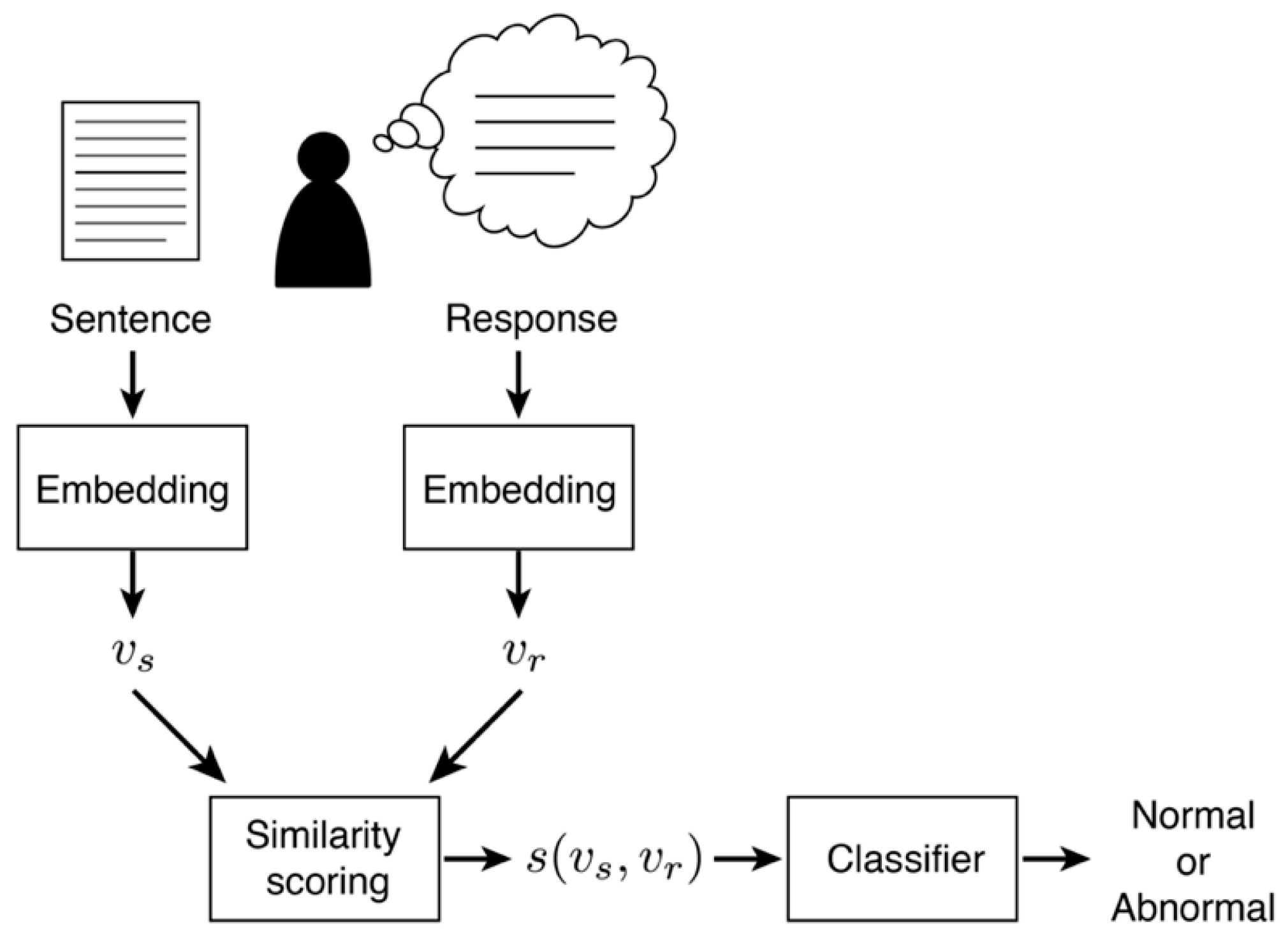
2.3. Feature Extraction
2.4. Classification Models
2.5. Classification Accuracy Measured Using Cross-Validation
3. Results
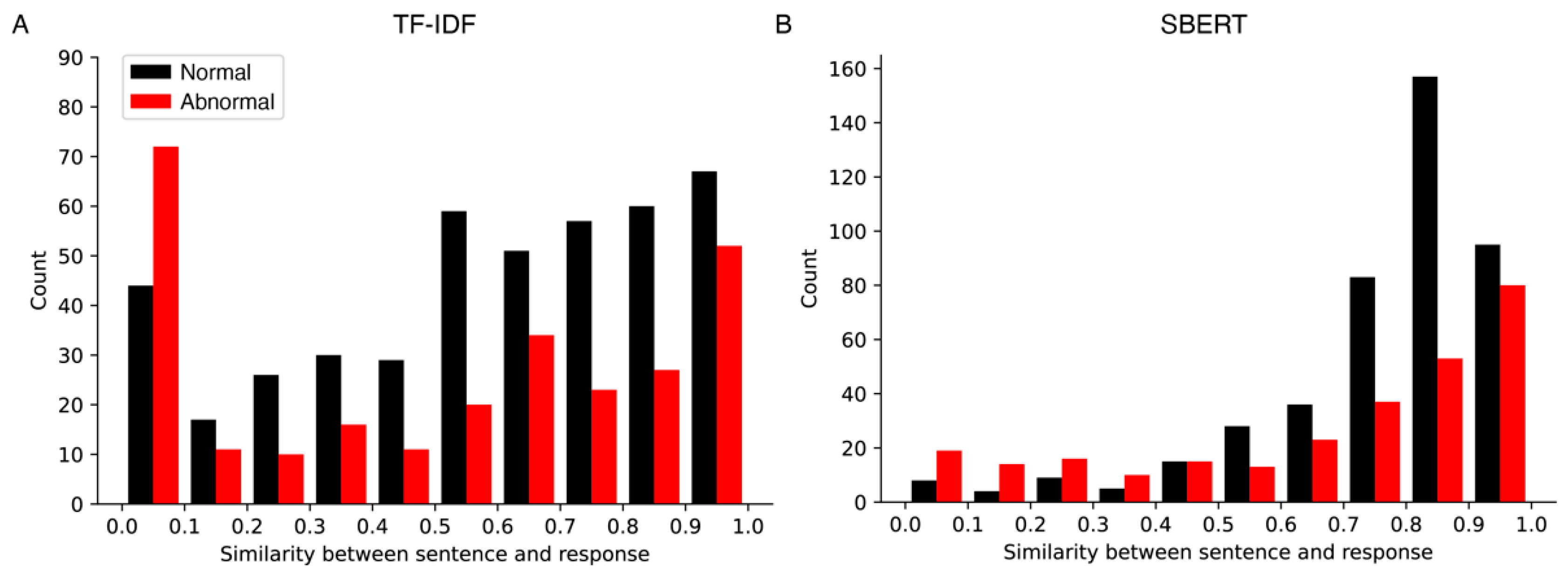
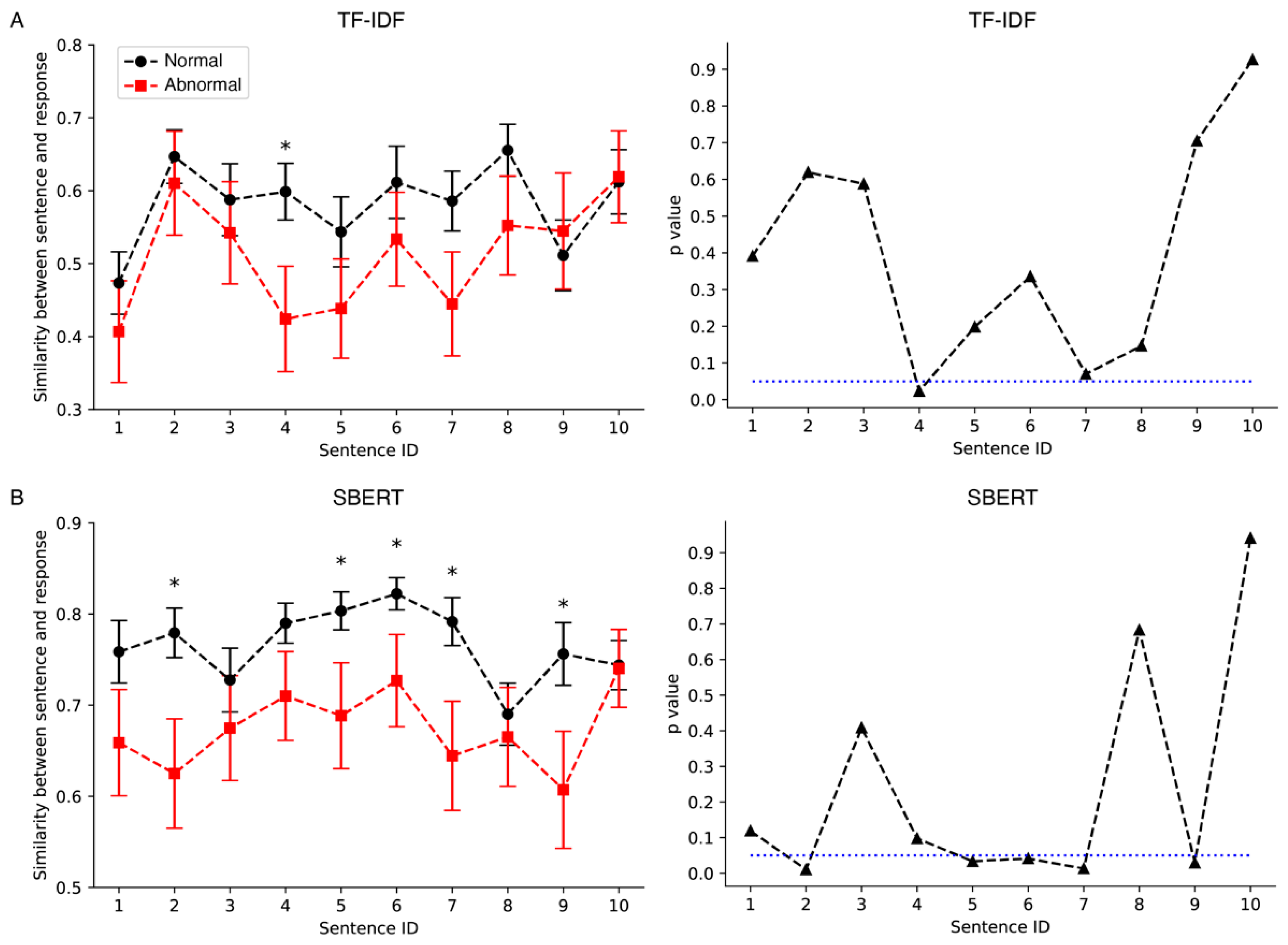
3.1. Similarity Scores
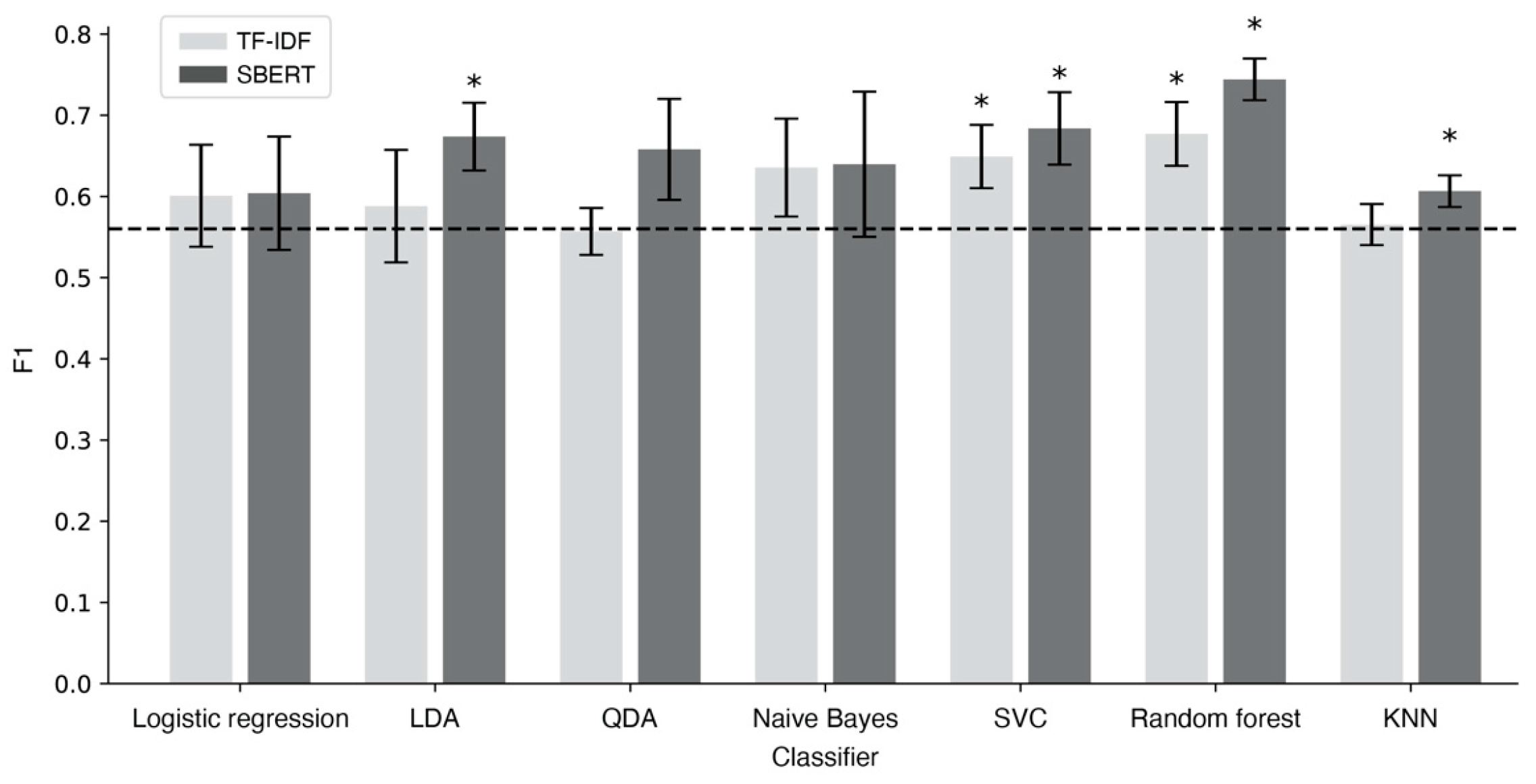
3.2. Classification Accuracies
4. Discussion
5. Conclusions
Funding
Institutional Review Board Statement
Informed Consent Statement
Data Availability Statement
Conflicts of Interest
References
- Snowling, M.J.; Hulme, C. The Science of Reading: A Handbook; Blackwell Publishing: Oxford, UK, 2005. [Google Scholar]
- American Psychiatric Association. Diagnostic and Statistical Manual of Mental Disorders, 5th Edition: DSM-5; American Psychiatric Publishing: Washington, DC, USA, 2013. [Google Scholar]
- Hulme, C.; Snowling, M.J. Developmental Disorders of Language Learning and Cognition; John Wiley & Sons: West Sussex, UK, 2013. [Google Scholar]
- Fletcher, J.M.; Lyon, G.R.; Fuchs, L.S.; Barnes, M.A. Learning Disabilities: From Identification to Intervention, 2nd ed.; Guilford Press: New York, NY, USA, 2018. [Google Scholar]
- Pressley, M.; Afflerbach, P. Verbal Protocols of Reading; Routledge: New York, NY, USA, 1995. [Google Scholar]
- Riazi, A.M. The Routledge Encyclopedia of Research Methods in Applied Linguistics; Routledge: New York, NY, USA, 2016. [Google Scholar]
- Bowles, M.A. The Think-Aloud Controversy in Second Language Research; Routledge: New York, NY, USA, 2010. [Google Scholar]
- Jurafsky, D.; Martin, J.H. Speech and Language Processing, 2nd ed.; Prentice Hall: Hoboken, NJ, USA, 2008. [Google Scholar]
- Zhang, Y.; Jin, R.; Zhou, Z.H. Understanding bag-of-words model: A statistical framework. Int. J. Mach. Learn. Cybern. 2010, 1, 43–52. [Google Scholar] [CrossRef]
- Aizawa, A. An information-theoretic perspective of TF–IDF measures. Inf. Process. Manag. 2003, 39, 45–65. [Google Scholar] [CrossRef]
- Bengio, Y.; Ducharme, R.; Vincent, P.; Jauvin, C. A neural probabilistic language model. J. Mach. Learn. Res. 2003, 3, 1137–1155. [Google Scholar]
- Mikolov, T.; Sutskever, I.; Chen, K.; Corrado, G.S.; Dean, J. Distributed representations of words and phrases and their compositionality. Adv. Neural Inf. Process. Syst. 2013, 26, 1–9. [Google Scholar]
- Pennington, J.; Socher, R.; Manning, C.D. GloVe: Global vectors for word representation. In Proceedings of the 2014 Conference on Empirical Methods in Natural Language Processing (EMNLP), Doha, Qatar, 25–29 October 2014; Stanford University: Stanford, CA, USA, 2014; pp. 1532–1543. [Google Scholar]
- Le, Q.; Mikolov, T. Distributed Representations of Sentences and Documents. In Proceedings of the 31st International Conference on Machine Learning, Beijing, China, 21–26 June 2014; Available online: https://portal.issn.org/resource/ISSN/1938-7288 (accessed on 15 December 2023).
- Reimers, N.; Gurevych, I. Sentence-BERT: Sentence Embeddings using Siamese BERT-Networks. In Proceedings of the 2019 Conference on Empirical Methods in Natural Language Processing and the 9th International Joint Conference on Natural Language Processing (EMNLP-IJCNLP), Hong Kong, China, 3–7 November 2019; pp. 3982–3992. [Google Scholar]
- Reimers, N.; Gurevych, I. Making monolingual sentence embeddings multilingual using knowledge distillation. In Proceedings of the 2020 Conference on Empirical Methods in Natural Language Processing (EMNLP), Online, 16–20 November 2020; pp. 4512–4525. [Google Scholar]
- Kim, A.; Kim, U.; Hwang, M.; Yoo, H. Test of Reading Achievement and Reading Cognitive Processes Ability (RA-RCP); Hakjisa: Seoul, Republic of Korea, 2014. [Google Scholar]
- Choi, M.; Hur, J.; Jang, M.-G. Constructing Korean lexical concept network for encyclopedia question-answering system. In Proceedings of the 30th Annual Conference of IEEE Industrial Electronics Society, Busan, Republic of Korea, 2–6 November 2004; Volume 3, pp. 3115–3119. [Google Scholar]
- Yun, H.; Sim, G.; Seok, J. Stock Prices Prediction using the Title of Newspaper Articles with Korean Natural Language Processing. In Proceedings of the International Conference on Artificial Intelligence in Information and Communication, Okinawa, Japan, 11–13 February 2019; pp. 19–21. [Google Scholar]
- Open-Source Korean Text Processor. Available online: https://github.com/open-korean-text/open-korean-text (accessed on 12 July 2023).
- Vaswani, A.; Shazeer, N.; Parmar, N.; Uszkoreit, J.; Jones, L.; Gomez, A.N.; Kaiser, L.; Polosukhin, I. Attention is all you need. Adv. Neural Inf. Process. Syst. 2017, 30, 1–11. [Google Scholar]
- Park, S.; Moon, J.; Kim, S.; Cho, W.I.; Han, J.; Park, J.; Song, C.; Kim, J.; Song, Y.; Oh, T.; et al. KLUE: Korean language understanding evaluation. arXiv 2021, arXiv:2105.09680. [Google Scholar]
- Liu, Y.; Ott, M.; Goyal, N.; Du, J.; Joshi, M.; Chen, D.; Levy, O.; Lewis, M.; Zettlemoyer, L.; Stoyanov, V. RoBERTa: A robustly optimized BERT pretraining approach. arXiv 2019, arXiv:1907.11692. [Google Scholar]
- Ko-Sroberta-Multitask. Available online: https://huggingface.co/jhgan/ko-sroberta-multitask (accessed on 20 July 2023).
- Ham, J.; Choe, Y.J.; Park, K.; Choi, I.; Soh, H. KorNLI and KorSTS: New benchmark datasets for Korean natural language understanding. arXiv 2020, arXiv:2004.03289. [Google Scholar]
- KorNLU Datasets. Available online: https://github.com/kakaobrain/kor-nlu-datasets (accessed on 20 July 2023).
- Cox, D.R. The regression analysis of binary sequences. J. R. Stat. Soc. Ser. B (Methodol.) 1958, 20, 215–232. [Google Scholar] [CrossRef]
- Fisher, R.A. The use of multiple measurements in taxonomic problems. Ann. Eugen. 1936, 7, 179–188. [Google Scholar] [CrossRef]
- Anderson, T.W. An Introduction to Multivariate Statistical Analysis, 3rd ed.; John Wiley & Sons: Hoboken, NJ, USA, 2003. [Google Scholar]
- Domingos, P.; Pazzani, M. On the optimality of the simple Bayesian classifier under zero-one loss. Mach. Learn. 1997, 29, 103–130. [Google Scholar] [CrossRef]
- Cortes, C.; Vapnik, V. Support-vector networks. Mach. Learn. 1995, 20, 273–297. [Google Scholar] [CrossRef]
- Breiman, L. Random forest. Mach. Learn. 2001, 45, 5–32. [Google Scholar] [CrossRef]
- Cover, T.; Hart, P. Nearest neighbor pattern classification. IEEE Trans. Inf. Theory 1967, 13, 21–27. [Google Scholar] [CrossRef]
- Hastie, T.; Tibshirani, R.; Friedman, J.H.; Friedman, J.H. The Elements of Statistical Learning, 2nd ed.; Springer: New York, NY, USA, 2009. [Google Scholar]


Disclaimer/Publisher’s Note: The statements, opinions and data contained in all publications are solely those of the individual author(s) and contributor(s) and not of MDPI and/or the editor(s). MDPI and/or the editor(s) disclaim responsibility for any injury to people or property resulting from any ideas, methods, instructions or products referred to in the content. |
© 2024 by the author. Licensee MDPI, Basel, Switzerland. This article is an open access article distributed under the terms and conditions of the Creative Commons Attribution (CC BY) license (https://creativecommons.org/licenses/by/4.0/).
Share and Cite
Yoo, Y. Automated Think-Aloud Protocol for Identifying Students with Reading Comprehension Impairment Using Sentence Embedding. Appl. Sci. 2024, 14, 858. https://doi.org/10.3390/app14020858
Yoo Y. Automated Think-Aloud Protocol for Identifying Students with Reading Comprehension Impairment Using Sentence Embedding. Applied Sciences. 2024; 14(2):858. https://doi.org/10.3390/app14020858
Chicago/Turabian StyleYoo, Yongseok. 2024. "Automated Think-Aloud Protocol for Identifying Students with Reading Comprehension Impairment Using Sentence Embedding" Applied Sciences 14, no. 2: 858. https://doi.org/10.3390/app14020858
APA StyleYoo, Y. (2024). Automated Think-Aloud Protocol for Identifying Students with Reading Comprehension Impairment Using Sentence Embedding. Applied Sciences, 14(2), 858. https://doi.org/10.3390/app14020858