Study on High-Precision Tension Control Technology for a Cold-Rolling Pilot Mill with Hydraulic Tension

Abstract

Tension control in cold-rolling pilot mills (CRPMs) with hydraulic tension is subject to extraneous forces resulting from positional disturbances, strong coupling, and time-varying characteristics, making it challenging to achieve ideal control results using the existing control methods. Therefore, in this study, a mathematical model of tension is first derived and then used to analyze the properties and difficulties associated with tension control. Second, a hydraulic servo-control system based on servovalves and proportional pressure relief valves is developed. In this system, redundant feedforward flow is generated by a servovalve according to the rolling schedule. The surplus flow is absorbed by a proportional pressure relief valve in the closed-loop control of tension. Third, simulation analysis is performed. Under severe friction disturbance (maximum 0.2 kN), and with the wide range of forward and backward slip, an accuracy of ±0.27 kN in tension control can still be achieved using the proposed control strategy, thereby demonstrating its effectiveness. Moreover, it has obvious advantages over existing control methods. Finally, an experimental study of tension is carried out in the cold-rolling mill with a maximum tension capacity of 50 kN, achieving ±0.2 kN tension control precision in the multipass rolling process.

1. Introduction

CRPMs with hydraulic tension represent a key piece of experimental equipment to simulate the cold-rolling process. As shown in Figure 1, hydraulic cylinders on each side of the mill apply constant tension to the workpiece. For CRPMs with hydraulic tension, only a small piece of metal strip is used as a workpiece, so they have lower energy and material consumption than traditional CRPMs with coilers [1].

In the cold-rolling process, the tension can significantly reduce deformation resistance by changing the stress state of the deformation zone and reducing the longitudinal compressive stress. As a result, the tension directly influences the thickness accuracy, flatness, and surface quality. Therefore, in the cold-rolling process, the tension must be accurately controlled in order to obtain high-quality cold-rolled products [2,3,4]. However, the tension control for a CRPM with hydraulic tension has its own particularities and difficulties, as described in Section 2. First, the forward and backward tensions are coupled with each other. Second, tension cylinders are required to track the rolling speed while achieving closed-loop tension control in typical hydraulic load control systems, where there is strong extraneous force disturbance [5,6]. Third, the forward and backward tensions are affected by many factors, such as work roller radius, rolling speed, friction coefficient, pass reduction, the type of strip material and its geometric dimensions, etc. Fourth, the stiffness of the workpiece changes in real time. Last, limited by the stroke of the tension cylinder and the length of the strip, the rolling process is often in a stage of acceleration or deceleration, which is detrimental for tension control. Thus, how to ensure the stability of tension is the most critical technical issue that has to be solved in CRPMs with hydraulic tension.

Currently, the design of CRPMs with hydraulic cylinders is mostly finished by VATRON in Austria or Northeastern University in China. In the hydraulic design of VATRON, both the ring and piston sides of the tension cylinders are controlled by an independent servovalve. Damping holes are set between the ring sides and the oil-return pipeline, and damping holes are also set between the piston sides and the oil-return pipeline. The control system, with four servovalves, is flexible, but the controlled objects are coupled with each other, making the program very complex. In addition, the equipment is very expensive. The damping holes are set to eliminate excess force, but a large amount of high-pressure fluid will flow through them and back to the oil tank during work, resulting in huge amounts of noise and energy loss. Reports on tension control for CRPMs with hydraulic cylinders are mainly from Northeastern University in China. Zhang designed a method to realize constant tension control with proportional pressure relief valves [7] (marked as method 1). During the rolling process, the outlet of the hydraulic pump is directly connected with the ring side of the entry tension cylinder through pipelines, and constant tension control is achieved through the proportional relief valve. However, due to the impact of the high-frequency flow pulsation of the pump and the fluid inertia effect [8,9], the accuracy of tension control is limited. Furthermore, when used to control T_H, the flow of the proportional relief valve includes the pump flow and the output flow from the entry-tension cylinder, which makes it necessary to designate a large nominal size (at least 10 mm) for the proportional relief valves. It can be seen from the user manual that the larger the nominal size of the valve, the slower its response speed, thereby affecting the dynamic effect of tension control. In order to solve the problems existing in the above method, Sun provided a control technique combining a speed feedforward controller with a tension feedback controller [10] (marked as method 2). The servovalves are directly installed on the ring sides of the tension cylinders, and the feedforward calculation method of the servovalve flow can effectively eliminate the influence of pump pressure fluctuation and the pipeline effect, which significantly improves the tension control accuracy. However, this method is reliant on the accurate prediction of forward and backward slip. If the predictions of forward and backward slip are inaccurate, there will be large tension deviation. The forward and backward slip are related to the material, reduction rate, friction coefficient, and roller diameter, among many other factors. This makes accurate prediction difficult, especially when variable gauge rolling is carried out [11]. The uncertainty of forward and backward slip greatly affects the accuracy of tension control.

Furthermore, there has also been much research on extraneous force compensation in electric–hydraulic load simulators. Jing Huang et al. derived the exact mathematical model of the control system, proposed the parameter-adaptive sliding-mode force control based on the reaching law and carried out experimental research. Their results fully demonstrated the effectiveness of the control method [12]. Guichao Yang and Jianyong Yao proposed an innovative multilayer neuroadaptive controller to further improve the output force tracking performance of electro–hydraulic load simulators with uncertainty rejection, where closed-loop stability is guaranteed, and extensive comparative application results were achieved [13]. Chenghu Jing et al. proposed a novel system for dynamic surface disturbance rejection control with synchronous compensation to improve the torque tracking performance of electro–hydraulic load simulators, resulting in a closed-loop system with high precision and robustness [6]. Shuo Kang et al. proposed an almost disturbance decoupling control strategy for solving the force control problem of an electro–hydraulic load simulator containing mechanical backlash. Both their simulation and experimental results demonstrated the advantages of the proposed control method [5]. However, the stiffness of the clamped object in the electro–hydraulic load simulator remained unchanged during the entire working process. The stiffness of the CRPM workpiece constantly changes at both the exit and the entry side of the rolling mill. In addition, forward and backward tension are established by the rolling mill and two tension cylinders, respectively, so the uncertainty of forward and backward slip in the rolling process results in a more complicated tension control process than in electro–hydraulic load simulators. Therefore, it is difficult to achieve the ideal tension control effect in CRPMs when using the method applied in electro–hydraulic load simulators.

As can be seen, the robustness of the existing techniques is not strong, and the control results are unsatisfactory. It is therefore essential to propose a new strategy for improving the robustness and control precision of tension control.

In this paper, tension models are first established, and the difficulties of tension control are analyzed in Section 2. Then, a new type of tension control strategy is proposed in Section 3. Next, simulation analysis and the field application are carried out to prove the effectiveness and advancement of the proposed control strategy in Section 4 and Section 5. Finally, the conclusions are drawn in Section 6.

2. Tension Modeling and Its Analysis

2.1. Tension Modeling

A demonstration of tension application during the rolling process is shown in Figure 2. A is the exit clamp center. B is the steady rolling zone center. C is the entry clamp center. l₂ is the transient distance between B and C. x_a, x_b, and x_c are, respectively, the displacements of A, B, and C. T_h is the forward tension. T_H is the backward tension. h is the exit thickness. H is the entry thickness.

It can be concluded from the geometric relationship that the strain of the strip under the increment of forward tension is

$$\epsilon =\frac{x_{\mathrm{a}}-x_{\mathrm{b}}}{l_{0\mathrm{h}}+x_{\mathrm{b}}}$$

(1)

where l_0h is the equivalent original length of the workpiece on the exit side.

According to Hooke’s law, when the material undergoes elastic deformation, the stress and the strain satisfy the equation

$$T_{\mathrm{h}}-T_{0\mathrm{h}}=E\epsilon A_{\mathrm{h}}$$

(2)

where E is the elastic modulus of the material; T_0h is the initial forward tension before rolling; A_h is the cross-sectional area of the strip on the exit side.

According to the Delhi Princeton formula, forward slip can be expressed as

$$S_{\mathrm{h}}=\frac{{\gamma }^2}{h}R$$

(3)

where $\gamma$ is a neutral angle; R is the roller radius.

The neutral angle is obtained according to the force balance condition of the rolling zone [14]

$$\gamma =\frac{\alpha }{2}(1-\frac{\alpha }{2f})+\frac{T_{\mathrm{h}}-T_{\mathrm{H}}}{4\overline{p}fwR}$$

(4)

where f is the friction coefficient; w is the width of the strip; $\overline{p}$ is the average rolling pressure; $\alpha ={\cos }^{-1}(\frac{R-\Delta h}{R})$; $\Delta h$ is the pass reduction.

By substituting Equation (4) into Equation (3), the following equation is obtained:

$$S_{\mathrm{h}}=\frac{{[\frac{\alpha }{2}(1-\frac{\alpha }{2f})+\frac{T_{\mathrm{h}}-T_{\mathrm{H}}}{4\overline{p}fwR}]}^2}{h}R$$

(5)

According to the definition of the forward slip, the exit speed is

$$v_{\mathrm{b}}=v(1+S_{\mathrm{h}})$$

(6)

where v is the rolling speed of the mill.

Integrating both sides of Equation (6), x_b can be obtained as

$$x_{\mathrm{b}}={\displaystyle {\int }_0^{t}v(1+S_{\mathrm{h}})} \mathrm{d}t$$

(7)

By substituting Equations (1) and (7) into Equation (2), the following equation is obtained:

$$T_{\mathrm{h}}=\frac{A_{\mathrm{h}}E}{l_{0\mathrm{h}}+{\displaystyle {\int }_0^{t}v(1+S_{\mathrm{h}})} \mathrm{d}t}[x_{\mathrm{a}}-{\displaystyle {\int }_0^{t}v(1+S_{\mathrm{h}})} \mathrm{d}t]+T_{0\mathrm{h}}$$

(8)

Combining Equation (8) with the principle of metal second flow being equal, the back slip model is obtained. The backward tension differential equation can then be obtained using the same method mentioned above.

$$T_{\mathrm{H}}=\frac{A_{\mathrm{H}}E}{l_{0\mathrm{H}}-\frac{h}{H}{\displaystyle {\int }_0^{t}v(1+S_{\mathrm{h}})} \mathrm{d}t}[\frac{h}{H}{\displaystyle {\int }_0^{t}v(1+S_{\mathrm{h}})} \mathrm{d}t-x_{\mathrm{c}}]+T_{0\mathrm{H}}$$

(9)

where l_0H is the equivalent original length of the workpiece on the entry side; T_0H is the initial backward tension before rolling. From the above modeling process, the block diagram of the tension model can be derived, as shown in Figure 3.

2.2. Tension Control Analysis

Equations (8) and (9) show that the forward and backward tension are influenced by numerous factors during the rolling process, mainly as described in the following:

(1)

The forward and backward tension are coupled with each other. The reason is that the workpiece is rolled by rollers while simultaneously being pulled by tension. A plastic deformation region is formed while rolling, and the forward and backward tensions are then coupled together because of their effects on neutral angle γ.

(2)

The forward and backward tensions are affected by numerous factors such as work roller radius R, rolling speed v, friction coefficient f, pass reduction $\Delta h$, the type of workpiece material and its geometric dimensions, etc.

(3)

The tension cylinders must match the rolling speed while maintaining constant forward and backward tension. Therefore, tension control is a typical load-control process with excess force from strong positional disturbances [15,16,17]. Only the tension feedback closed-loop controller is incapable of meeting the requirements for synchronizing the speed between the hydraulic cylinders and the workpiece while also maintaining the stability of tension.

(4)

The lengths l₁ and l₂ between the clamps and the rollers, shown in Figure 2, are closely related to the displacement of the left and right tension cylinders. During rolling, these change in real time, which causes the tension control system to have properties of variable stiffness, which greatly increases the difficulty of tension control.

In summary, achieving high-precision tension control for CRPMs with hydraulic tension represents a challenging problem. A satisfactory control effect cannot be obtained using conventional hydraulic circuits and control methods, making it necessary to design and develop both a new tension control platform and control method.

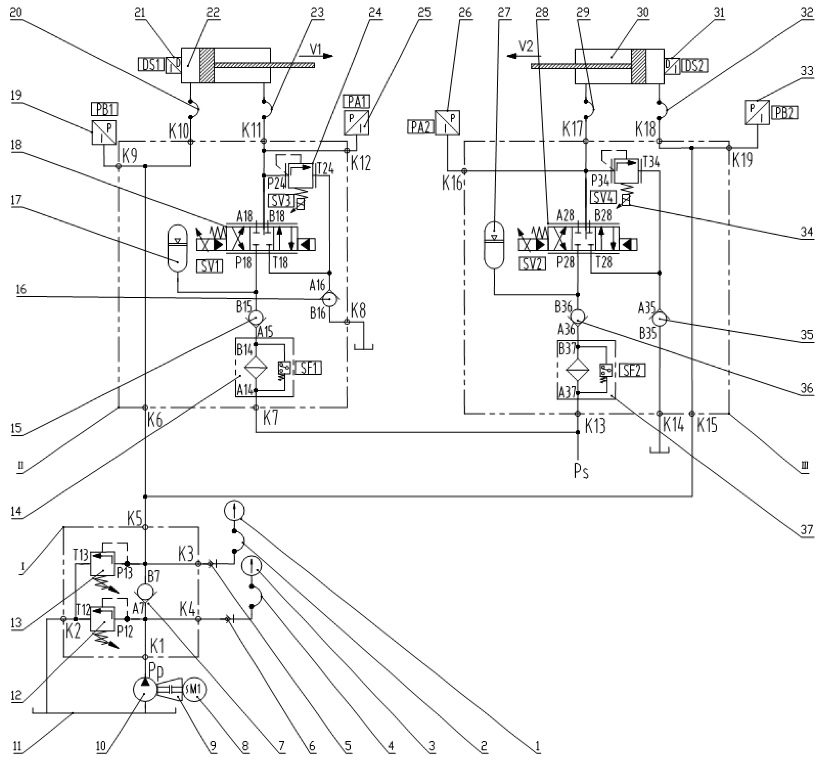
3. Designing a New Hydraulic Platform and Control Method

3.1. Designing a New Hydraulic Platform

The newly designed hydraulic circuit diagram is shown in Figure 4. It includes control devices for constant back pressure and left and right tension.

Considering the property of the rolling process where one side cylinder always extends while the other retracts, the piston sides of the two tension cylinders and the outlet of the constant back pressure control device are connected together. In this way, the working flow of the piston sides can complement each other. The constant back pressure device mainly consists of a check valve and two identical relief valves. The adjustment method and the working principle are: (1) The setting pressures of the two relief valves are manually adjusted to Py₁₁ and Py₁₂, and Py₁₁ = Py₁₂ (ignoring the pressure drop generated when the oil flows through the first check valve). Assuming the flows through the two relief valves are Qy₁₁ and Qy₁₂, then Qy₁₁ = Qy₁₂ because the two relief valves have the same specifications. (2) When tension cylinders work in position control mode, the mill is not in a rolling state, so the pressure fluctuations in the piston sides do not influence the tension control results. (3) In rolling state, both tension cylinders work in force control mode. When the rolling speed is zero, the output fluid of the fixed displacement pump will flow through two relief valves, and the pressure in the piston chambers of the tension cylinders will be Py₁₁.

When the rolling speed is not zero, taking the rolling direction from left to right as an example, the left tension cylinder is on the entry side and has speed v_H = (1 – S_H)v. The right tension cylinder is on the exit side and has speed v_h = (1 + S_h)v. Obviously, v_h > v_H, and the speed difference is (S_h + S_H)v. The speed difference causes excess fluid to flow back into the constant back pressure control device through K5, and this flow is Q_g = (S_h + S_H)vA_w, where A_w is the effective area of the ring side. Assuming the flow through the first relief valve is Qy₂₁, the inlet pressure of first relief valve is P₂₁, the flow through the second relief valve is Qy₂₂, the inlet pressure of the second relief valve is P₂₂, and ignoring the internal and external leakage of the tension control cylinders, we obtain

$$Q_{\mathrm{p}}=Q{y}_{11}+Q{y}_{12}$$

(10)

where Q_p is the output flow of the fixed displacement pump. Then,

$$Q{y}_{21}+Q{y}_{22}=Q_{\mathrm{p}}+Q_{\mathrm{g}}$$

(11)

With Equations (10) and (11), and Qy₁₁ = Qy₁₂, we obtain

$$Q{y}_{22}-Q{y}_{12}=Q_{\mathrm{g}}+(Q{y}_{12}-Q{y}_{21})$$

(12)

Ignoring the pressure drop caused by the first check valve, we get P₂₁ = P₂₂ and

$$Q{y}_{21}=Q{y}_{22}$$

(13)

With Equations (11) and (13), the variation in the flow through the second relief valve is

$$Q{y}_{22}-Q{y}_{12}=0.5Q_{\mathrm{g}}=0.5(S_{\mathrm{h}}+S_{\mathrm{H}})v{A}_{\mathrm{w}}$$

(14)

Generally speaking, S_h < 5% and S_H < 45%. Then, the variation in the flow through the second relief valve is

$$Q{y}_{22}-Q{y}_{12}<0.25v{A}_{\mathrm{w}}$$

(15)

This is far less than the output flow (1 + S_h) vA_w from the piston side of the exit tension cylinder, which is very helpful in reducing the pressure fluctuations of the piston sides.

The same conclusions are obtained when the direction of rolling is from right to left.

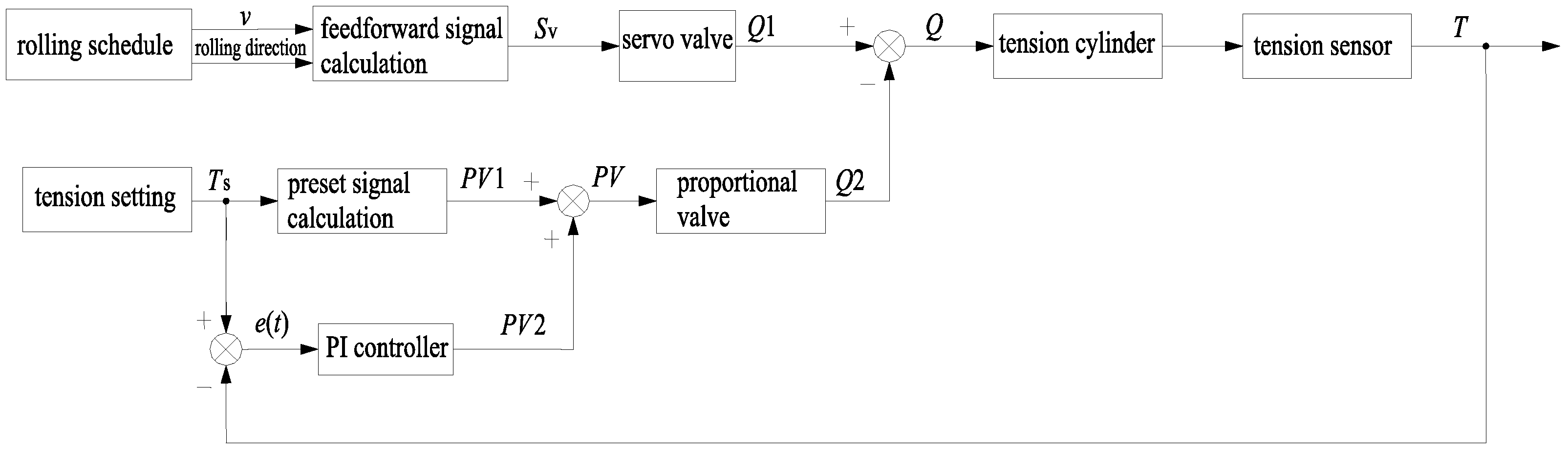
3.2. Control Strategy for the Left and Right Tension Control Devices

The left and right tension control devices mainly consist of filters, accumulators, servovalves, and proportional pressure relief valves. The accumulators are used to maintain a stable operating pressure in the supply pressure port (P) of the servovalves. During rolling, tension is mainly controlled by servovalves and proportional pressure relief valves. The control principle for each tension cylinder is shown as Figure 5. With the feedforward method, the servovalve provides feedforward flow Q1 to the ring side of the tension cylinder. For the ring side of the exit side tension cylinder, the feedforward flow is always more than the required input flow. The excess flow is absorbed by the exit side proportional pressure relief valve to ensure the exit side tension remains stable. For the ring side of the entry side tension cylinder, the feedforward flow is always less than the actual output flow. The excess flow is absorbed by the entry side proportional pressure relief valve to ensure the entry side tension remains stable.

3.2.1. The Feedforward Control Method for Servovalves

First, the speed and direction of rolling can be determined according to the rolling schedule. The next step is to calculate the feedforward signals for servovalves. The actual flow depends on the displacement of the spool and the valve pressure drop. For different values of valve pressure drop, the flow may be calculated by the square root function for a sharp-edged orifice [18]:

$$Q=Q_{\mathrm{N}}\frac{x_{\mathrm{v}}}{x_{\max }}\sqrt{\frac{\Delta P}{\Delta P_{\mathrm{N}}}}$$

(16)

where ΔP is the actual valve pressure drop; x_v is the displacement of the spool; x_max is the maximum displacement of the spool; ΔP_N is the rated valve pressure drop; Q_N is the rated flow. With regard to the entry side servovalve, ΔP = P₁, where P₁ is the actual pressure of valve port A. With regard to the exit side servovalve, ΔP = P_s – P₁, where P_s is the working supply pressure of the valve. Note that ΔP in Equation (16) is the total pressure drop including P→A and B→T (or P→B and A→T), 50% each. In the newly designed system, the servovalve is used as a two-edged valve, so the valve pressure drop is simply P→A or B→T. Therefore, the relation between valve flow and the displacement of the spool is

$$Q=Q_{\mathrm{N}}\frac{x_{\mathrm{v}}}{x_{\max }}\sqrt{\frac{\Delta P}{0.5\Delta P_{\mathrm{N}}}}$$

(17)

In addition, the displacement of the spool is proportional to the electric command signal. We obtain

$$\frac{S_{\mathrm{v}}}{S_{\mathrm{v}\max }}=\frac{Q}{Q_{\mathrm{N}}}\sqrt{\frac{0.5\Delta P_{\mathrm{N}}}{\Delta P}}$$

(18)

where S_v is the electric command signal; S_vmax is the maximum electric command signal. In Equation (18), the parameters such as ΔP_N, Q_N, and S_vmax can be easily determined from the valve manual. The calculation of ΔP requires P_s and P₁. P_s and P₁ can be obtained from pressure sensors. Therefore, S_v can be calculated when we obtain Q, which is related to rolling speed, forward slip, and backward slip. The forward slip value in the cold-rolling process is usually less than 5%, so the electric command signal for the exit side servovalve is set as

$$S_{\mathrm{vh}}=S_{\mathrm{v}\max }\frac{1.05vA}{Q_{\mathrm{N}}}\sqrt{\frac{0.5\Delta P_{\mathrm{N}}}{\Delta P}}$$

(19)

where A is the ring area of the tension cylinder. In this way, the valve flow certainly exceeds the required input flow. The excess flow is absorbed by the exit side proportional pressure relief valve, and the relief flow satisfies

$$Q_{\mathrm{ph}}<S_{\mathrm{v}\max }\frac{0.05vA}{Q_{\mathrm{N}}}\sqrt{\frac{0.5\Delta P_{\mathrm{N}}}{\Delta P}}$$

(20)

In this way, the adjusted relief flow range is much smaller than that in [7] under the same working conditions.

The backward slip value in the cold-rolling process is usually less than 45%, so the electric command signal for the entry side servovalve is set as

$$S_{\mathrm{vH}}=S_{\mathrm{v}\max }\frac{0.55vA}{Q_{\mathrm{N}}}\sqrt{\frac{0.5\Delta P_{\mathrm{N}}}{\Delta P}}$$

(21)

In this way, the valve flow is certainly less than the actual output flow from the ring side of the entry side tension cylinder. The excess flow is absorbed by the corresponding proportional pressure relief valve to keep the tension stable, and the relief flow satisfies

$$Q_{\mathrm{pH}}<S_{\mathrm{v}\max }\frac{0.45vA}{Q_{\mathrm{N}}}\sqrt{\frac{0.5\Delta P_{\mathrm{N}}}{\Delta P}}$$

(22)

In this way, the adjusted relief flow range is much smaller than that in [7] under the same working conditions. All in all, the adjusted flow ranges of the proportional pressure relief valves are markedly reduced by the feedforward flow effect of the servovalves. This is very helpful for achieving better tension control using proportional pressure relief valves.

3.2.2. The Control Method for Proportional Pressure Relief Valves

As shown in Figure 4, the preset signal of the proportional pressure relief valve can be calculated from the preset tension. The real-time adjusting signal of the proportional pressure relief valve is determined by a PI controller according to the error e(t) between the preset and actual tension, which forms the closed-loop controller. The output of the PI controller is

$$P{V}_2=K_{\mathrm{p}}[e(t)+\frac{1}{T_{\mathrm{i}}}{\displaystyle {\int }_0^{t}e(t)\mathrm{d}t}]$$

(23)

where K_p is proportional gain; T_i is integral time.

The sum of preset signal and PI controller output is the actual command signal for the proportional pressure relief valve. Based on the static force balance condition of the left tension cylinder, the preset signal of the left proportional pressure relief valve can be calculated as

$$P{V}_{11}=\frac{T_1+P_0{A}_2}{A_1}\cdot \frac{P{V}_{\mathrm{N}}}{P_{\mathrm{N}}}$$

(24)

where T₁ is left preset tension; P₀ is the constant pressure on the piston side; A₁ is the ring area of the cylinder; A₂ is the piston area of the cylinder; PV_N is the rated command signal; P_N is the rated adjusting pressure. The difference between the preset and actual left tension value is input to the PI controller, and its output is PV₂₁. Hence, the actual command signal for left proportional pressure relief valve is PV₁ = PV₁₁ + PV₂₁.

Based on the static force balance condition of the right tension cylinder, the preset signal of the right proportional pressure relief valve can be calculated as

$$P{V}_{12}=\frac{T_2+P_0{A}_2}{A_1}\cdot \frac{P{V}_{\mathrm{N}}}{P_{\mathrm{N}}}$$

(25)

where T₂ is the right preset tension. The difference between the preset and actual right tension value is input to the PI controller, and its output is PV₂₂. Hence, the actual command signal for the right proportional pressure relief valve is PV₂ = PV₁₂ + PV₂₂.

4. Simulation Analysis

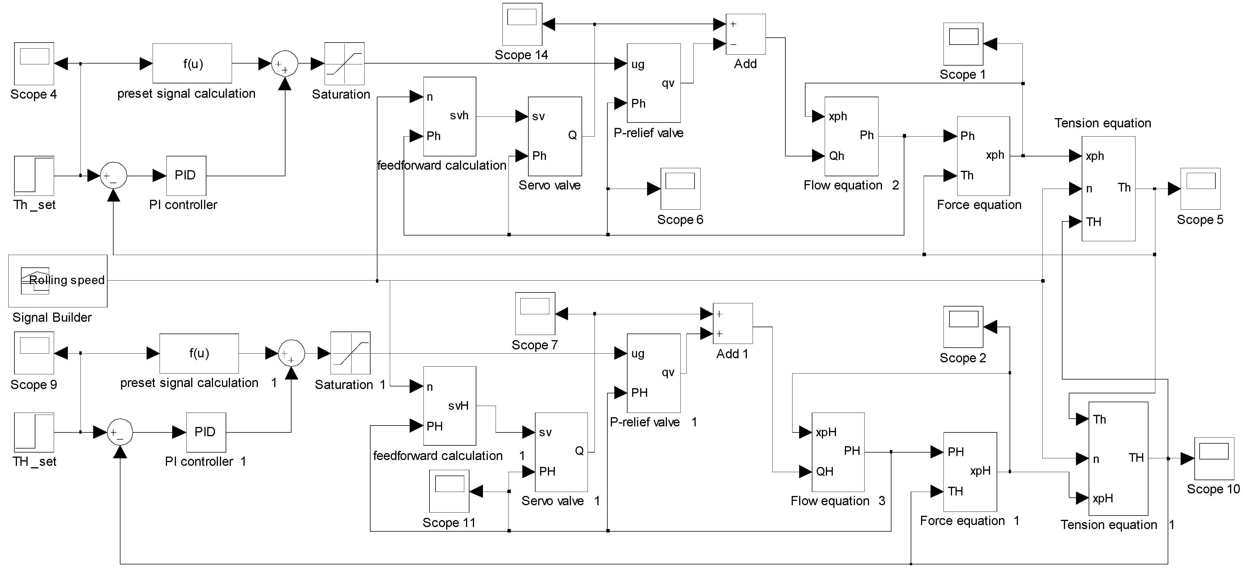
4.1. Modeling of Hydraulic Tension Control System

The dynamic characteristics of the tension control system are highly nonlinear. The nonlinearities arise from the compressibility of the hydraulic fluid, the complex flow properties of the servovalves, and the friction of the tension cylinders. In order to build the model of the system, firstly, the following assumptions are made:

(1)

The supply pressure of the servovalves is constant, while the return flow is fed to a tank under the return pressure 0;

(2)

The oil pressure is evenly distributed at each side of the cylinders, and the temperature of the oil is constant;

(3)

The bulk modulus of the oil is a constant.

4.1.1. Servovalve Modeling

A servovalve is a complex component having high-order dynamic characteristics. Its dynamic characteristics are influenced by many factors such as oil pressure, input signal, and oil temperature, among others. Therefore, only approximations are acquired, even though a high-order transfer function is used to describe the dynamic characteristics of the servovalve. However, in most hydraulic systems, the servovalve has a much higher dynamic response speed than the load. Therefore, when analyzing the dynamic characteristics of the system, only knowledge of the dynamic characteristics of the servovalve in an appropriate low frequency range is required. In this study, the servovalve is treated as a second-order system, and its transfer function can be described as

$$\frac{Q(s)}{S_{\mathsf{v}}(s)}=\frac{K_{\mathrm{v}}}{\frac{s^2}{{\omega }_{\mathrm{n}}{}^2}+\frac{2\zeta }{{\omega }_{\mathrm{n}}}s+1}\sqrt{\Delta p}$$

(26)

where $K_{\mathrm{v}}=\frac{Q_{\mathrm{N}}}{S_{\mathrm{v}\max }\sqrt{0.5\Delta p_{\mathrm{N}}}}$; ${\omega }_{\mathrm{n}}$ is the undamped natural frequency; $\zeta$ is the damping ratio; $\Delta p=\left\{\begin{array}{c}{P}_s-P_1 I\ge 0\\ P_1 I<0\end{array}\right.$.

4.1.2. Modeling of Proportional Relief Valve

A proportional relief valve is used for converting electrical input signals into a proportional pressure output signal, as well as for limiting the pressure. A schematic representation of a proportional relief valve is shown in Figure 6.

The dynamics of the proportional solenoid coil can be described as [19]

$$L\frac{\mathrm{d}i}{\mathrm{d}t}=k_{\mathrm{D}3}{u}_{\mathrm{g}}-(k_{\mathrm{D}3}{k}_{\mathrm{D}4}+R)i$$

(27)

where R is the sum of the coil resistance and the amplifier resistance; L is the coil inductance; k_D3 is the amplifier voltage amplification factor; u_g is the amplifier input voltage; k_D4 is the current feedback gain of the proportional solenoid.

The relief valve is normally closed. When the pressure setting of the valve is reached, the equation describing the spool motion is

$$P_{1}A=m_1\frac{{\mathrm{d}}^{2}y}{\mathrm{d}{t}^2}+f_1\frac{\mathrm{d}y}{\mathrm{d}t}+k_{\mathrm{D}1}i+k_{\mathrm{D}2}y+k_{\mathrm{e}1}y{P}_1$$

(28)

where A is the spool side area; m₁ is the spool mass; f₁ is the damping coefficient; k_e1 is the hydrodynamic stiffness of the valve port; y is the spool displacement; P₁ is the inlet pressure of the valve; k_D1 is current force gain factor of the proportional solenoid; i is the drive current of the valve; k_D2 is the spring stiffness.

The opening area of the valve is calculated as

$$A_{\mathrm{open}}=\pi y\sin \frac{\alpha }{2}\left(D_1-\frac{y}{2}\sin \alpha \right)$$

(29)

where D₁ is the valve seat diameter. The opening area is bounded by the maximum displacement y_max

$$y_{\max }=\frac{D_1\left(1-\sqrt{1-\cos \frac{\alpha }{2}}\right)}{\sin \alpha }$$

For any needle displacement larger than y_max, A_open is the maximum orifice area

$$A_{\mathrm{open}}=\frac{\pi }{4}{D}_1{}^2$$

The flow equation of the relief valve can be described as

$$q_{\mathrm{v}}=C_{\mathrm{d}2}\pi D_{1}y\sin \frac{\alpha }{2}\left(D_1-\frac{y}{2}\sin \alpha \right)\sqrt{\frac{2}{\rho }{P}_1}+\frac{V_1}{{\beta }_{\mathrm{e}}}\frac{\mathrm{d}{P}_1}{\mathrm{d}t}+A\frac{\mathrm{d}y}{\mathrm{d}t}$$

(30)

where q_v is the overflow through the relief valve; ρ is the density of fluid; β_e is the bulk modulus of fluid; V₁ is the volume of the working chamber in the valve; C_d2 is the flow coefficient of the valve port; D₁ is the valve seat diameter; α is the taper angle of the spool.

4.1.3. Flow Equations for Hydraulic Tension Cylinders

Considering the internal and external leakage, the flow equation for the ring side of the exit tension cylinder is

$$Q_{\mathrm{h}}=A_1\frac{\mathrm{d}{x}_{\mathrm{ph}}}{\mathrm{d}t}+\frac{V_{1\mathrm{h}}}{{\beta }_{\mathrm{e}}}\frac{\mathrm{d}{P}_{\mathrm{h}}}{\mathrm{d}t}+C_{\mathrm{iph}}(P_{\mathrm{h}}-P_0)+C_{\mathrm{eph}}{P}_{\mathrm{h}}$$

(31)

where Q_h is the flow into the ring side of the cylinder; x_ph is the displacement of the cylinder; V_1h is the real-time volume of the ring side; C_iph is the internal leakage coefficient of the cylinder; C_eph is the external leakage coefficient of the cylinder; P_h is the pressure in ring side; P₀ is the constant pressure in piston side.

Considering the internal and external leakage, the compressible oil flow continuity equation for the ring side of the entry tension cylinder is

$$A_1\frac{\mathrm{d}{x}_{\mathrm{pH}}}{\mathrm{d}t}=Q_{\mathrm{H}}+\frac{V_{1\mathrm{H}}}{{\beta }_{\mathrm{e}}}\frac{\mathrm{d}{P}_{\mathrm{H}}}{\mathrm{d}t}+C_{\mathrm{ipH}}(P_{\mathrm{H}}-P_0)+C_{\mathrm{epH}}{P}_{\mathrm{H}}$$

(32)

where Q_H is the flow into the ring side of the cylinder; x_pH is the displacement of the cylinder; V_1H is the volume of the ring side of the cylinder; C_ipH is the internal leakage coefficient of the cylinder; C_epH is the external leakage coefficient of the cylinder; P_H is the pressure of the ring side of the cylinder.

4.1.4. Motion Equations of the Hydraulic Tension Cylinders

The motion equation of the exit tension cylinder is

$$A_1{P}_{\mathrm{h}}-A_2{P}_0=M_{\mathrm{th}}\frac{{\mathrm{d}}^2{x}_{\mathrm{ph}}}{\mathrm{d}{t}^2}+B_{\mathrm{ph}}\frac{\mathrm{d}{x}_{\mathrm{ph}}}{\mathrm{d}t}+T_{\mathrm{h}}+f_{\mathrm{h}}$$

(33)

where M_th is the total mass of the cylinder’s movable part and the exit clamp, ignoring the mass of the strip; T_h is the forward tension; B_ph is the viscous friction coefficient of the cylinder; f_h is the Coulomb friction.

The motion equation of the entry tension cylinder is

$$A_2{P}_0+T_{\mathrm{H}}-A_1{P}_{\mathrm{H}}=M_{\mathrm{tH}}\frac{{\mathrm{d}}^2{x}_{\mathrm{pH}}}{\mathrm{d}{t}^2}+B_{\mathrm{pH}}\frac{\mathrm{d}{x}_{\mathrm{pH}}}{\mathrm{d}t}+f_{\mathrm{H}}$$

(34)

where M_tH is the total mass of the cylinder’s movable part and the entry clamp, ignoring the mass of the strip; T_H is the backward tension; B_pH is the viscous friction coefficient; f_H is the Coulomb friction.

4.1.5. Integrated Model of Tension Control System

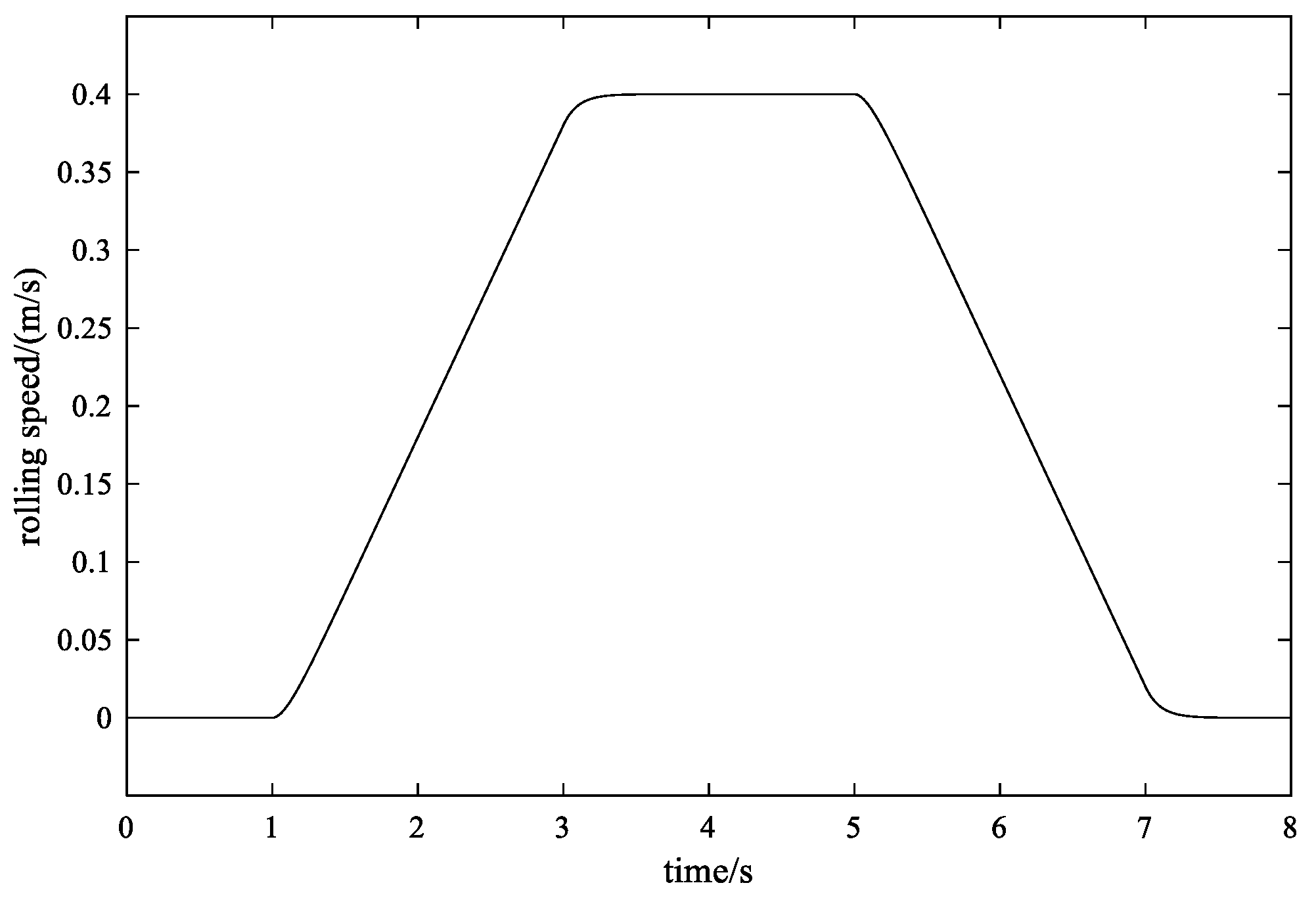
Considering all the above analyses, the integrated model of the tension control system can be obtained as shown in Figure 7. The modeling and simulation software used in this paper is Simulink R2021a. Some key parameters of the model are K_v = 1.069 × 10⁻⁷ m³/(s·mA·Pa^0.5); ω_n = 250 rad/s; ζ = 0.707; P_s = 21 MPa; β_e = 1500 MPa; M_th = M_tH = 150 kg; B_ph = B_pH = 100 N/(m/s); ρ = 900 kg/m³; A₁ = 0.0032 m²; A₂ = 0.0064 m²; H = 0.2 mm; h = 0.16 mm. With this configuration, the tension cylinders can achieve a maximum tension of 50 kN.

4.2. Simulation

The set rolling speed is shown in Figure 8, where 0–1 s is the static stage; 1–3 s is the accelerating stage, and the rolling speed increases from 0 to 0.4 m/s; 3–5 s is the uniform speed stage; 5–7 s is the descending stage, and the speed returns to 0 at 7 s. During the whole process, the set forward tension is 15 kN, and the set backward tension is 20 kN. Friction disturbance is an important factor affecting the accuracy of tension control. It is set as shown in Figure 9, covering the acceleration stage, uniform speed stage, and deceleration stage. Three methods (method 1, method 2, and the proposed method) are used for simulation. By adjusting the model shown in Figure 7, it is easy to derive the required simulation model using the first two methods, which will not be repeated in this paper.

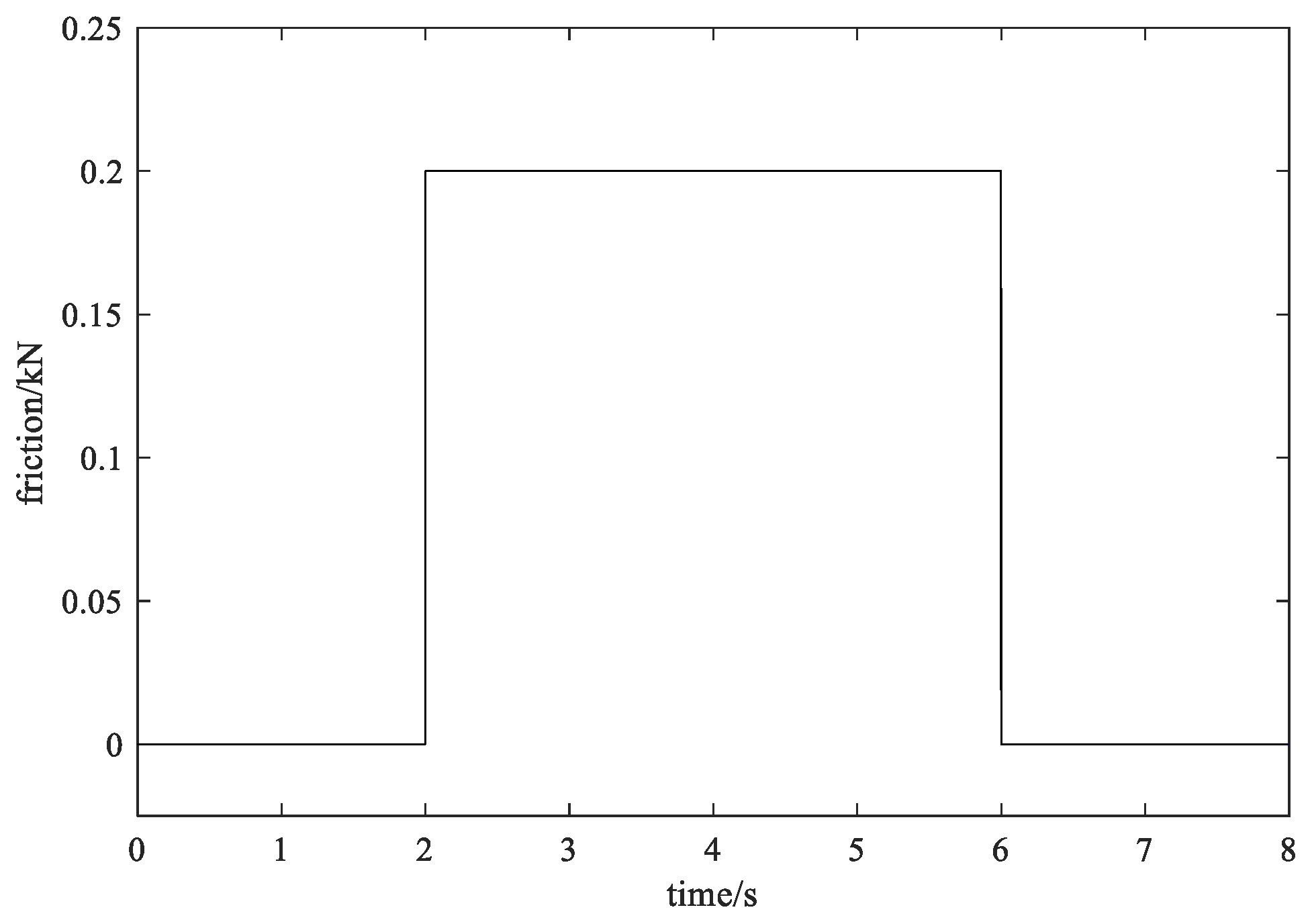
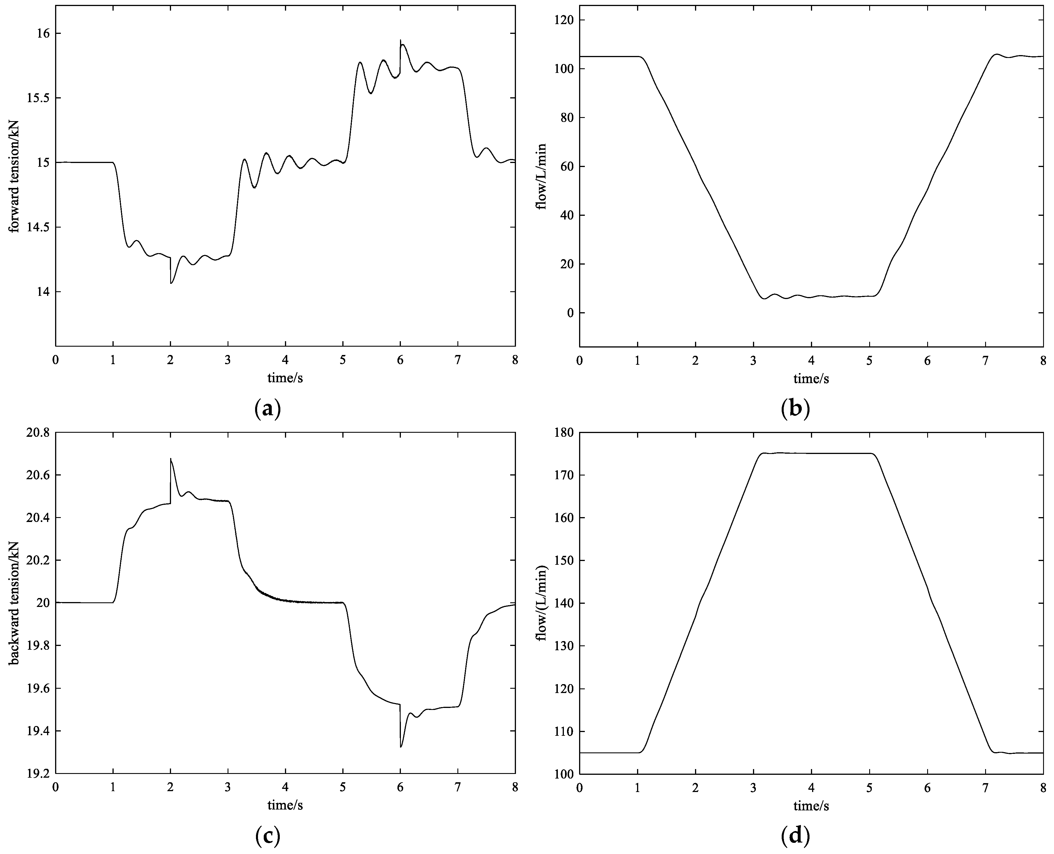
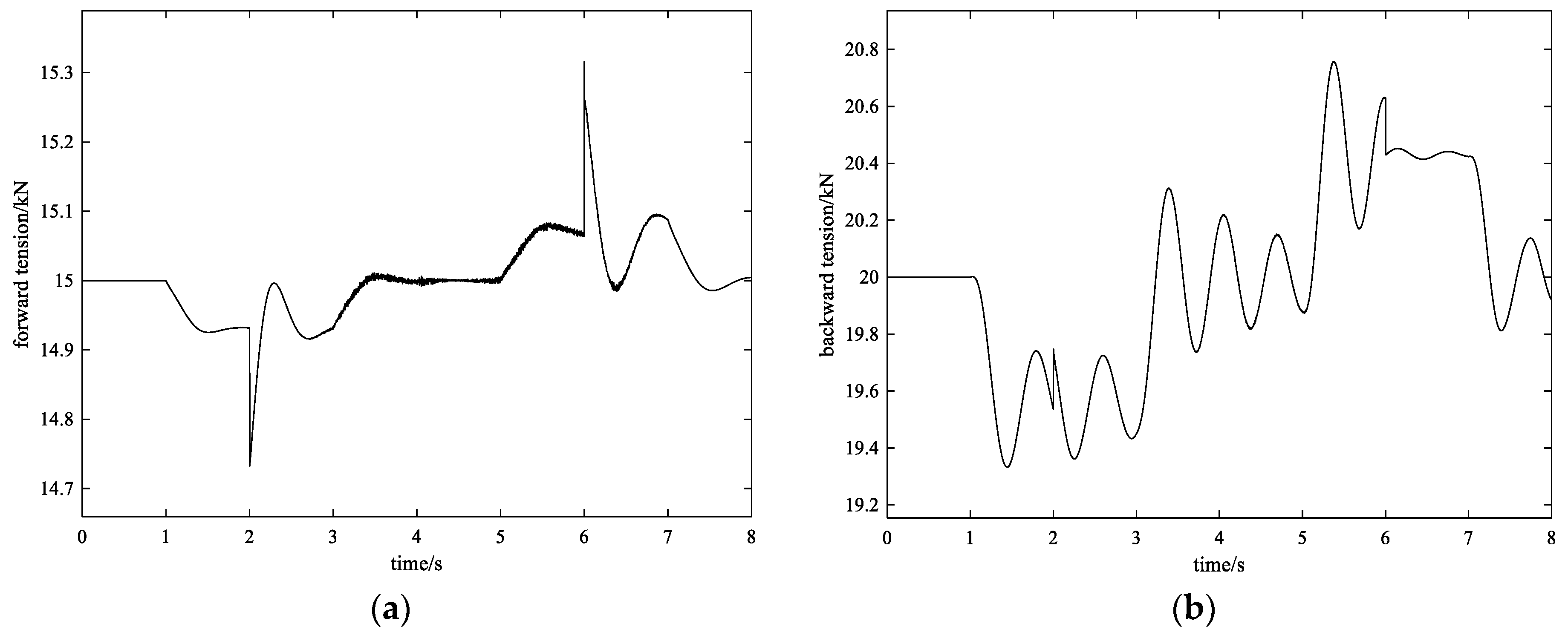
4.2.1. Control Effect with Method 1

When only used to control T_H, the flow of the proportional relief valve includes the pump flow and the output flow from the entry tension cylinder, which makes it necessary to select a large nominal size for the proportional relief valves. Here, the proportional relief valve with a rated flow rate of 200 L/min is selected. In addition, the volume of the chamber controlled by the proportional relief valve includes the volume of the pipeline from the outlet of the hydraulic pump to the ring side of the tension cylinder, which is counted as 0.01 m³. When S_h = 0.01 and S_H = 0.1, the tension control effect and the flow through the proportional relief valves are shown in Figure 10. When S_h = 0.04 and S_H = 0.4, the tension control effect and the flow through the proportional relief valves are shown in Figure 11.

As can be seen, when S_h = 0.01 and S_H = 0.1, the accuracy of forward tension control is ±1 kN, and the flow through the proportional relief valve on the exit side varies from 105 L/min to 9 L/min; the accuracy of backward tension control is ±0.7 kN, and the flow through the proportional relief valve on the entry side varies from 105 L/min to 175 L/min. When S_h = 0.04 and S_H = 0.4, there is little change in both the control accuracy of the forward tension control and the flow through the proportional relief valve on the exit side; the accuracy of the backward tension control is ±0.53 kN, and the flow through the proportional relief valve on the entry side varies from 105 L/min to 153 L/min. The flow adjustment range of the proportional relief valve on the entry side is reduced, and the control accuracy of T_H is improved.

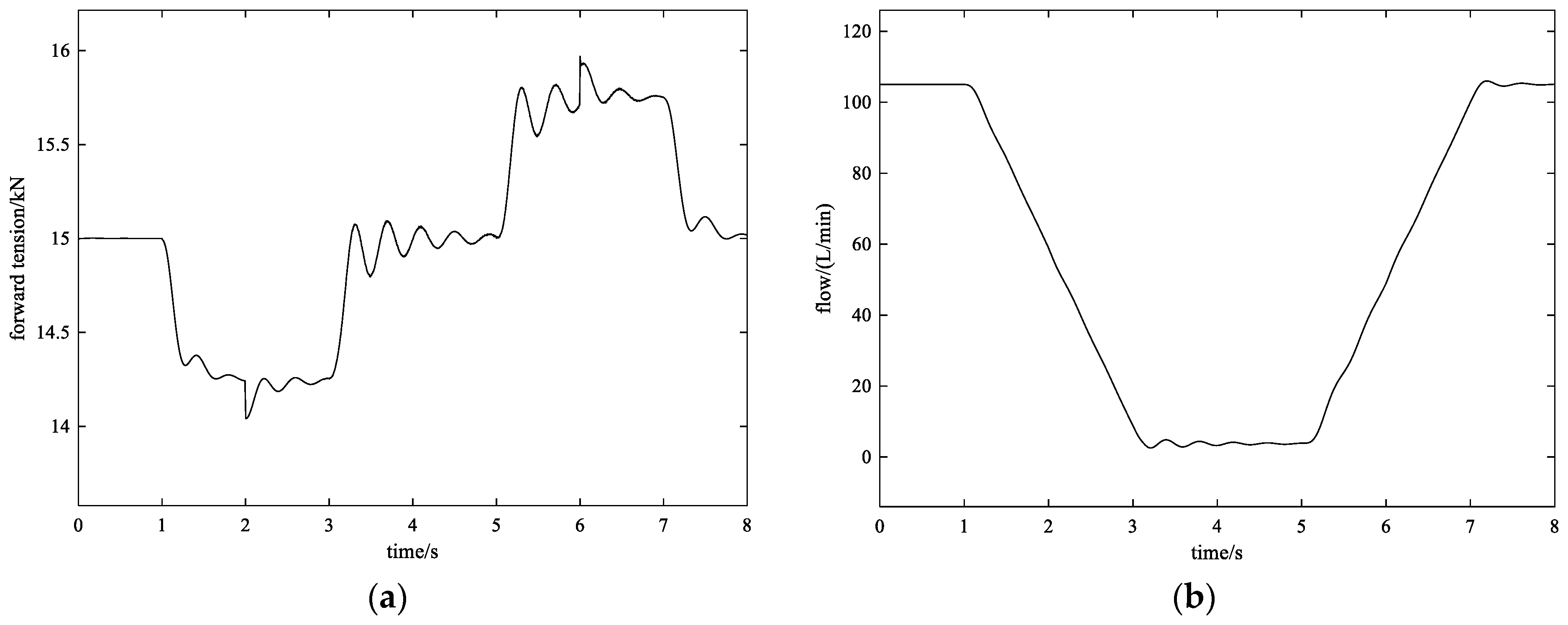
4.2.2. Control Effect with Method 2

If the prediction of forward slip and backward slip is accurate, high-precision tension control results can be achieved using method 2. Using the same rolling process as described above, the tension control effect with method 2 is shown in Figure 12. As can be seen, the maximum forward tension error is about −0.26 kN, and the maximum backward tension error is about −0.2 kN. The reason is that by using the feedforward speed, the roll rotation can be accurately tracked based on the speed of the tension cylinder, and thus the servovalve achieves equivalent tension closed-loop control under conditions where the rolls are static. The response speed of the servovalve is very high, so it achieves satisfactory tension closed-loop control accuracy.

However, the forward and backward slip are related to the material, reduction rate, friction coefficient, and roller diameter, among many other factors. This makes accurate prediction difficult, especially when variable gauge rolling is carried out. Assuming that the forward slip prediction value is 0.01 and the actual value is 0.04, and the backward slip prediction value is 0.1 and the actual value is 0.4, the control effect using method 2 is shown in Figure 13. It can be seen that the maximum error of the forward tension control is about −0.32 kN, and the maximum error of backward tension control is about −0.78 kN. The control accuracy is significantly reduced. The reason for this is that when there is a large error in the prediction of forward or backward slip, the tension cylinder cannot accurately track the roll rotation. There is high load stiffness in the tension closed loop, so the values of its controller parameters are low, which does not allow complete elimination of deviations between the tension cylinders and the roll rotation, resulting in large tension control errors.

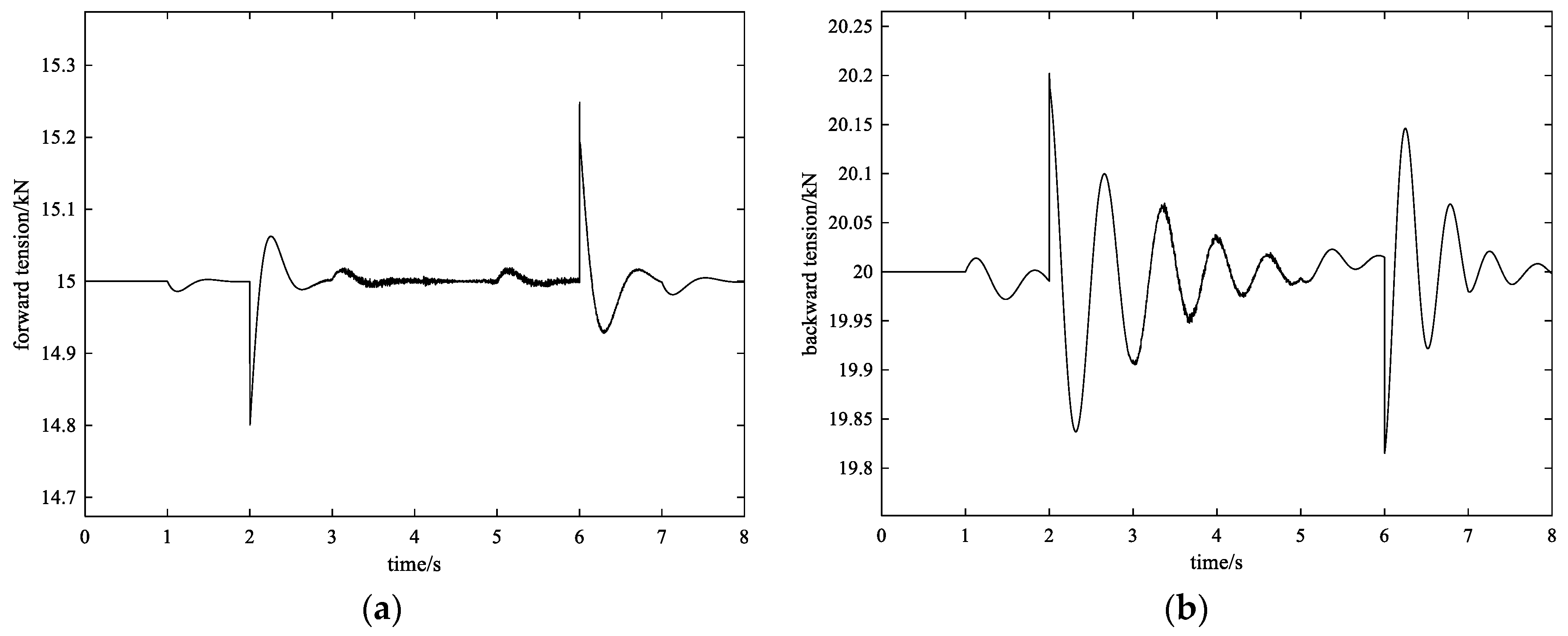
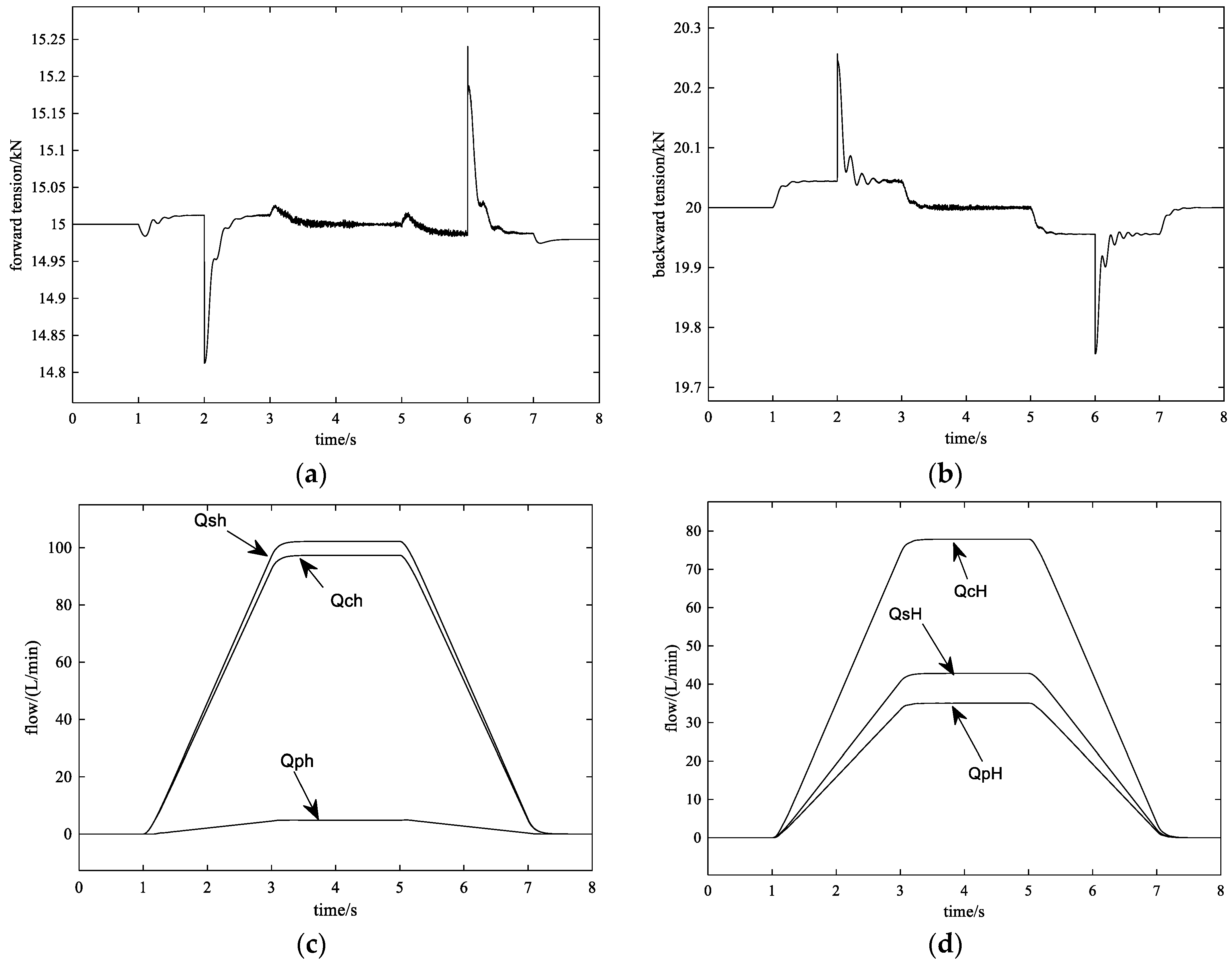
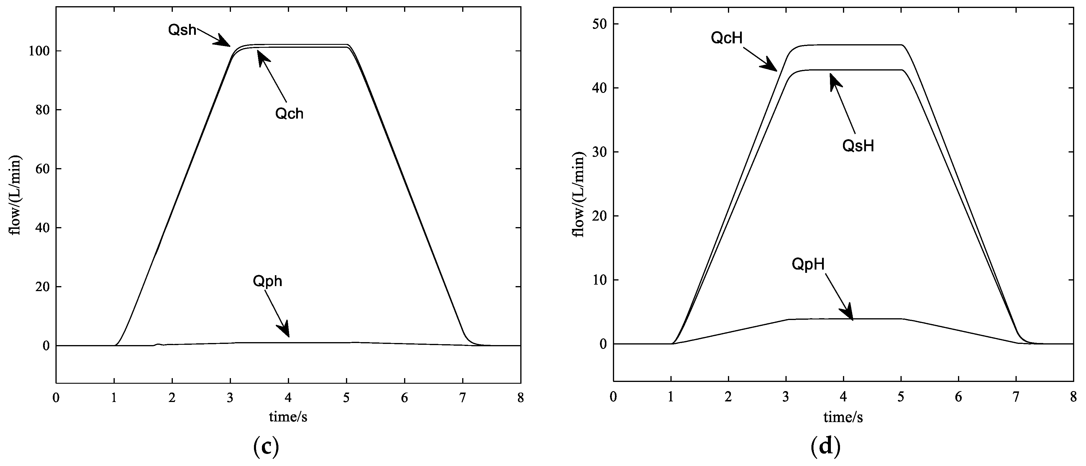
4.2.3. Control Effect with the Proposed Method

Using the proposed method, proportional relief valves with a nominal size of 6 mm and rated flow of 40 L/min are selected. Assuming that the forward slip S_h = 0.01 and the backward slip S_H = 0.1, the tension control results from using the proposed control strategy are shown in Figure 14, where Q_sh is the flow through the exit servovalve; Q_ch is the flow into the ring side of the exit cylinder; Q_ph is the flow through the exit proportional relief valve; Q_sH is the flow through the entry servovalve; Q_cH is the flow out of the ring side of the entry cylinder; Q_pH is the flow through the entry proportional relief valve. From the working principle of the hydraulic system, Q_ph = Q_sh − Q_ch, Q_pH = Q_cH − Q_sH. The largest forward tension error is about −0.25 kN, and the largest backward tension error is about −0.27 kN.

Assuming that forward slip S_h = 0.04 and backward slip S_H = 0.4, the tension control results obtained using the proposed method are shown in Figure 15. Even though the values for forward and backward slip have changed greatly, the tension control effect maintains high accuracy. Comparing Figure 14c with Figure 15c, with the increase in the forward slip, Q_ch increases and Q_sh remains unchanged, resulting in Q_ph decreasing. Comparing Figure 14d with Figure 15d, it can be seen that Q_cH decreases with the increase in backward slip and Q_sH remains unchanged, resulting in Q_pH decreasing. Therefore, with a wide range of forward and backward slip, the flow through the two proportional relief valves also changes but is always within the adjustable flow range of the proportional relief valves, and the valves with a small nominal size have a high response speed. Therefore, accuracy in tension control is guaranteed.

Compared with method 1, in the proposed method, the proportional relief valves require a much smaller flow adjustment range and a smaller nominal size, which allows them to have a faster response speed. In addition, the tension control is not affected by the fluid inertia effect present in method 1, so there is better tension control when using the proposed method.

Compared with method 2, the proposed method uses proportional pressure valves for tension control and is not dependent on the accurate prediction of forward and backward slip. Even when the forward and backward slip vary over a wide range, good tension control accuracy is maintained, and the method exhibits stronger robustness.

5. Application

The tension control strategy developed in this paper was applied to a CRPM with hydraulic tension, which is shown in Figure 16. This mill can be used for research into the cold-rolling process and new product development of metal materials such as steel, pure titanium, titanium alloy, and other alloys. The main parameters of the equipment are shown in

Table 1. Main parameters of the equipment.

Index	Items	Parameters	Index	Items	Parameters
1	Dimensions of backup roll/mm	Φ480~450 × 350	9	Transmission mode	Work roll drive compound reducer + DC motor drive
2	Material of backup roll	Heat-resistant forged steel 9Cr2Mo, ESR, forging, roll surface hardness 70~76 HSD, tensile strength ≥ 755 MPa	10	Main motor	DC motor, 2 × 132 kW, 500 r/min, DC440 V/339 A, digital speed regulation system control
3	Dimensions of work roll/mm	Φ200~190 × 370	11	Rolling speed/(m/s)	With tension: 0~±0.4 m/s Without tension: 0~±0.6 m/s
4	Material of work roll	High speed steel 86CrMoV7-Hi, ESR, forging, roller surface hardness 90~95 HSD, tensile strength ≥ 755 MPa	12	Hydraulic oil source pressure/MPa	21
5	Balance mode of upper roll system	Hydraulic balance	13	HGC cylinder	φ400/φ320–80
6	Max. opening/mm	20	14	Max. rolling force/kN	5000
7	Strip clamping mode	Hydraulic clamp	15	Tension cylinder	φ90/φ63–2100
8	Roll-gap control mode	HGC servo control	16	Tension control range/kN	0.5~50

, where ESR is the abbreviation for electroslag redissolution; HSD stands for Shore hardness; HGC is the abbreviation for hydraulic gauge control.

Examples of left and right tension control equipment are shown in Figure 17 for the rolling of high-strength steel DP550. Dual phase steel with a tensile strength of 550 MPa grade (DP550) is widely used in automotive bodies due to its high strength, good ductility, continuous yield, low yield ratio, and other advantages. The rolling schedule is shown in

Table 2. Cold-rolling schedule for high-strength steel.

Dimensions/mm	Pass	Left Tension/kN	Right Tension/kN	Rolling Force /kN	Rolling Speed /m·s−1	Exit Thickness /mm	Reduction Rate /%
3.6 × 200 × 650	1	48	45	1460	0.15	2.768	23.11
	2	42	44	1623	0.15	2.067	25.33
	3	40	38	1537	0.15	1.556	24.72
	4	33	36	1590	0.20	1.197	23.06
	5	30	28	1256	0.4	1.017	15.05

. The tension control results are shown in Figure 18.

As can be seen, after five rolling passes, the specimen was rolled from 3.6 mm to 1.017 mm, with a total reduction of 71.75%. As the length of the specimen increased, the maximum rolling speed increased from 0.15 m/s to 0.4 m/s. During the multipass rolling process, the tension control error remained within ± 0.2 kN, which is better than in the simulation result because the friction force set in the simulation is very strict. Firstly, the friction force value of 0.2 kN is higher than the maximum friction force in the actual process. Moreover, the set friction force has a step change process from 0 to the maximum value and from the maximum value to 0, which will cause significant errors in tension. From the single pass tension control curve, the actual tension trend of the rolling process was consistent with the simulation process. When the rolling started or stopped, the forward tension showed a decreasing trend, and the backward tension showed an overshooting trend. When switching from the acceleration section to the uniform speed section or from the uniform speed section to the deceleration section, the forward tension showed an overshooting trend, while the backward tension showed a decreasing trend.

6. Conclusions

(1)

Tension modeling was conducted based on Hooke’s law and rolling theories. The model reflects tension control properties such as variable rigidity, tension coupling, and positional disturbances. This demonstrated that high-precision tension control is very difficult and the existing hydraulic control methods are not suitable.

(2)

In consideration of the mill properties, the piston sides of the left and right tension cylinders are connected together, and the back pressure is controlled by a constant back pressure control device. In this way, the relief flows are greatly reduced, which is beneficial for reducing fluctuations in the back pressure. Furthermore, because of the existence of back pressure, the use of proportional pressure relief valves enables the avoidance of dead and nonlinear zones while working, ultimately resulting in the achievement of high-precision tension control.

(3)

The feedforward control for servovalves can ensure the effective tracking of rolling speed regardless of forward and backward slip. The surplus flow is absorbed by the corresponding proportional pressure valve in the closed-loop tension control. This method is simple, reliable, and has strong robustness.

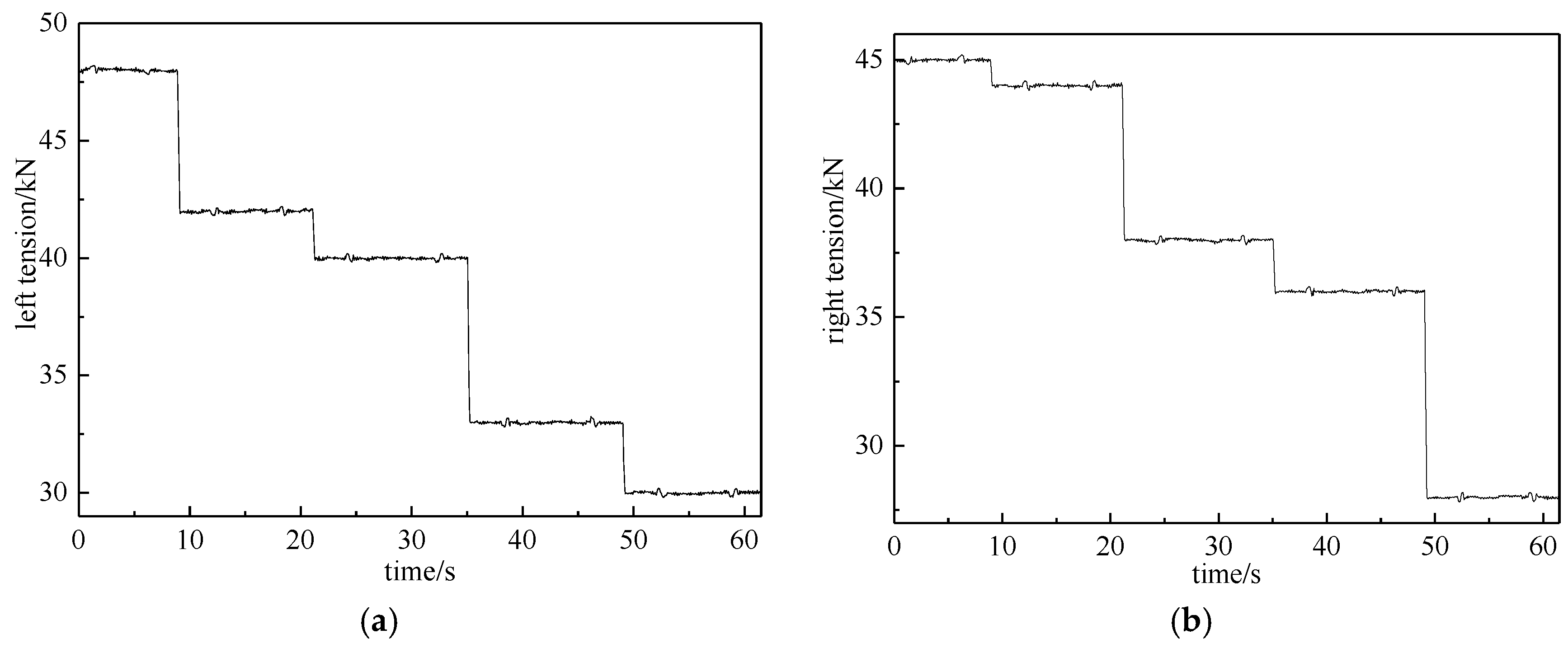
(4)

Based on a CRPM with 50 kN hydraulic tension, cold-rolling experiments were carried out on a typical metallic material. The dynamic tension control accuracy was controlled within ±0.2 kN, when the maximum rolling speed reached 0.4 m/s and the maximum single pass reduction reached 37%. Compared with the existing techniques, the proposed method has obvious advantages.

(5)

The hydraulic platform and the control method developed in this paper can serve as a helpful reference for the designs of hydraulic servo systems such as electro–hydraulic load simulators with positional disturbances.

(6)

The prerequisite for the effective use of the method proposed in this article is that the set rolling speed is known. Although the exit and entry speeds of the specimen are directly affected by forward and backward slip, the two factors are bounded. Therefore, the redundant flow generated by the feedforward of the servovalves is also bounded and can be adequately absorbed by the proportional relief valve, and an ideal tension control effect is achieved. For more complex working conditions, a strategy combining the optimization of hydraulic schematic design, the proposal of excellent control strategies and advanced algorithms, and improving the performance of the system components may be effective in further significantly suppressing the disturbances from extraneous forces.

References

1. Jiao, Z.J.; Li, J.P.; Zhang, F.B.; Wang, G.; Liu, X. Technological Design of New Type Pilot Cold Rolling Mill. Iron Steel 2007, 42, 53–55. (In Chinese) [Google Scholar]
2. Ozaki, K.; Ohtsuka, T.; Fujimoto, K.; Kitamura, A.; Nakayama, M. Nonlinear Receding Horizon Control of Thickness and Tension in a Tandem Cold Mill with a Variable Rolling Speed. ISIJ Int. 2012, 52, 87–95. [Google Scholar] [CrossRef]
3. Zhang, X.; Chen, S.; Zhang, H.; Zhang, X.W.; Zhang, D.H.; Sun, J. Modeling and Analysis of Interstand Tension Control in 6-high Tandem Cold Rolling Mill. J. Iron Steel Res. Int. 2014, 21, 830–836. [Google Scholar] [CrossRef]
4. Pittner, J.; Samaras, N.S.; Simaan, M.A. A new strategy for optimal control of continuous tandem cold metal rolling. IEEE Trans. Ind. Appl. 2010, 46, 703–711. [Google Scholar] [CrossRef]
5. Kang, S.; Nagamune, R.; Yan, H. Almost disturbance decoupling force control for the electro-hydraulic load simulator with mechanical backlash. Mech. Syst. Signal Process. 2020, 135, 106400. [Google Scholar] [CrossRef]
6. Jing, C.; Xu, H.; Jiang, J. Dynamic surface disturbance rejection control for electro-hydraulic load simulator. Mech. Syst. Signal Process. 2019, 134, 106293. [Google Scholar] [CrossRef]
7. Zhang, F.B.; Li, J.P.; Liu, X.H.; Wang, G.; Bi, Y.; Zou, J. A Hydraulic Proportional Control System to Achieve Constant Tension Control. Patent 200710010015.6, 8 August 2007. [Google Scholar]
8. Lin, J.; Wang, Y.; Zhou, S.; Wu, W.; Ma, H.; Han, Q. Simulation and experimental analysis of pressure pulsation characteristics of pump source fluid. Appl. Sci. 2021, 11, 9559. [Google Scholar] [CrossRef]
9. Krus, P.; Weddfelt, K.; Palmberm, J.-O. Fast pipeline models for simulation of hydraulic systems. J. Dyn. Syst. Meas. Control. 1994, 116, 132–136. [Google Scholar] [CrossRef]
10. Sun, T.; Wang, G.Q.; Wu, Y.; Zhang, H. Tension control technique for hydraulic-tension reversible experimental cold mill. J. Northeast. Univ. (Nat. Sci.) 2012, 33, 528–532. (In Chinese) [Google Scholar]
11. Liu, X.H. Prospects for variable gauge rolling technology, theory and application. J. Iron Steel Res. Int. 2011, 18, 1–7. [Google Scholar] [CrossRef]
12. Huang, J.; Song, Z.; Wu, J.; Guo, H.; Qiu, C.; Tan, Q. Parameter Adaptive Sliding Mode Force Control for Aerospace Electro-Hydraulic Load Simulator. Aerospace 2023, 10, 160. [Google Scholar] [CrossRef]
13. Yang, G.; Yao, J. Multilayer neuroadaptive force control of electro-hydraulic load simulators with uncertainty rejection. Appl. Soft Comput. 2022, 130, 109672. [Google Scholar] [CrossRef]
14. Wang, T.F.; Qi, K.M. Metal Plastic Processing: Rolling Theory and Technology, 2nd ed.; Metallurgical Industry Press: Beijing, China, 2001; pp. 40–45. (In Chinese) [Google Scholar]
15. Nam, Y.; Hong, S.K. Force control system design for aerodynamic load simulator. Control. Eng. Pract. 2002, 10, 549–558. [Google Scholar] [CrossRef]
16. Jianyong, Y.; Zongxia, J.; Yaoxing, S.; Cheng, H. Adaptive nonlinear optimal compensation control for electro-hydraulic load simulator. Chin. J. Aeronaut. 2010, 23, 720–733. [Google Scholar] [CrossRef]
17. Nam, Y. QFT force loop design for the aerodynamic load simulator. IEEE Trans. Aerosp. Electron. Syst. 2001, 37, 1384–1392. [Google Scholar]
18. Cao, X.M. Hydraulic Servo System; Metallurgical Industry Press: Beijing, China, 1991; pp. 14–18. (In Chinese) [Google Scholar]
19. Yao, J. Simulation frequency response characteristic of electro-hydraulic proportional relief valve based on Simulink. Hydraul. Pneum. Seals 2009, 29, 38–41. (In Chinese) [Google Scholar]
Figure 1. Schematic of a CRPM with hydraulic tension.
Applsci 14 00877 g001
Figure 2. Demonstration of tension loading.
Applsci 14 00877 g002
Figure 3. Block diagram representation of the tension model.
Applsci 14 00877 g003
Figure 4. Hydraulic circuit diagram of tension control: (1) first pressure gauge, (2) first pressure hose, (3) second pressure gauge, (4) second pressure hose, (5) first pressure joint, (6) second pressure joint, (7) first check valve, (8) electric motor, (9) coupling, (10) pump, (11) tank, (12) first pressure relief valve, (13) second pressure relief valve, (14) first filter, (15) second check valve, (16) third check valve, (17) first accumulator, (18) first servovalve, (19) first pressure sensor, (20) first hydraulic hose, (21) first displacement sensor, (22) left cylinder, (23) second hydraulic hose, (24) first proportional pressure relief valve, (25) second pressure sensor, (26) third pressure sensor, (27) second accumulator, (28) second servovalve, (29) third hydraulic hose, (30) right cylinder, (31) second displacement sensor, (32) fourth hydraulic hose, (33) fourth pressure sensor, (34) second proportional pressure relief valve, (35) fourth check valve, (36) fifth check valve, (37) second filter, (I) constant back pressure control device, (II) left tension control device, and (III) right tension control device.
Applsci 14 00877 g004
Figure 5. The tension control strategy diagram.
Applsci 14 00877 g005
Figure 6. Schematic representation of a proportional relief valve. 1: the housing; 2: proportional solenoid; 3: the valve seat; 4: the valve spool; 5: integrated amplifier.
Applsci 14 00877 g006
Figure 7. The integrated Simulink model.
Applsci 14 00877 g007
Figure 8. The setting curve of rolling speed.
Applsci 14 00877 g008
Figure 9. The set friction disturbance curve.
Applsci 14 00877 g009
Figure 10. The tension control effect and the flow through the proportional relief valves with method 1 when Sh = 0.01 and SH = 0.1. (a) The control effect of forward tension; (b) the flow through the proportional relief valve on the exit side; (c) the control effect of backward tension; (d) the flow through the proportional relief valve on the entry side.
Applsci 14 00877 g010
Figure 11. The tension control effect and the flow through the proportional relief valves with method 1 when Sh = 0.04 and SH = 0.4. (a) The control effect of forward tension; (b) the flow through the proportional relief valve on the exit side; (c) the control effect of backward tension; (d) the flow through the proportional relief valve on the entry side.
Applsci 14 00877 g011aApplsci 14 00877 g011b
Figure 12. The tension control effect with method 2 under accurate prediction of Sh and SH. (a) The control effect of forward tension; (b) the control effect of backward tension.
Applsci 14 00877 g012
Figure 13. The tension control effect with method 2 under inaccurate prediction of Sh and SH. (a) The control effect of forward tension; (b) the control effect of backward tension.
Applsci 14 00877 g013
Figure 14. The simulation results for tension control with the proposed method when Sh = 0.01 and SH = 0.1. (a) The control effect of forward tension; (b) the control effect of backward tension; (c) the flow curves on the exit side; (d) the flow curves on the entry side.
Applsci 14 00877 g014
Figure 15. The simulation results for tension control with the proposed method when Sh = 0.04 and SH = 0.4. (a) The control effect of forward tension; (b) the control effect of backward tension; (c) the flow curves on the exit side; (d) the flow curves on the entry side.
Applsci 14 00877 g015aApplsci 14 00877 g015b
Figure 16. Overall photo of the equipment.
Applsci 14 00877 g016
Figure 17. Left and right tension control equipment. (a) Left tension control equipment; (b) right tension control equipment.
Applsci 14 00877 g017
Figure 18. The actual tension control effect of the tension cylinders. (a) The control effect of left tension; (b) the control effect of right tension.
Applsci 14 00877 g018