Abstract
Improving the accuracy of parking space recognition is crucial in the fields for Automated Valet Parking (AVP) of autonomous driving. In AVP, accurate free space recognition significantly impacts the safety and comfort of both the vehicles and drivers. To enhance parking space recognition and annotation in unknown environments, this paper proposes an automatic parking space annotation approach with tight coupling of Lidar and Inertial Measurement Unit (IMU). First, the pose of the Lidar frame was tightly coupled with high-frequency IMU data to compensate for vehicle motion, reducing its impact on the pose transformation of the Lidar point cloud. Next, simultaneous localization and mapping (SLAM) were performed using the compensated Lidar frame. By extracting two-dimensional polarized edge features and planar features from the three-dimensional Lidar point cloud, a polarized Lidar odometry was constructed. The polarized Lidar odometry factor and loop closure factor were jointly optimized in the iSAM2. Finally, the pitch angle of the constructed local map was evaluated to filter out ground points, and the regions of interest (ROI) were projected onto a grid map. The free space between adjacent vehicle point clouds was assessed on the grid map using convex hull detection and straight-line fitting. The experiments were conducted on both local and open datasets. The proposed method achieved an average precision and recall of 98.89% and 98.79% on the local dataset, respectively; it also achieved 97.08% and 99.40% on the nuScenes dataset. And it reduced storage usage by 48.38% while ensuring running time. Comparative experiments on open datasets show that the proposed method can adapt to various scenarios and exhibits strong robustness.
1. Introduction
Automatic parking space detection is a crucial technical challenge in the fields of autonomous driving systems, surveying and mapping, security monitoring, and urban traffic management, as illustrated in Figure 1. Parking space recognition is used for automatic parking in Figure 1a and for parking lot mapping in Figure 1b. Additionally, autonomous driving systems require reliable parking space recognition and annotation capabilities to enable Automated Valet Parking (AVP) and enhance driving safety. AVP is a future vision for fully automated autonomous vehicles [1]. Parking space recognition is essential for guiding vehicles to park smoothly and accurately in Automatic Parking Assist Systems (APAS).
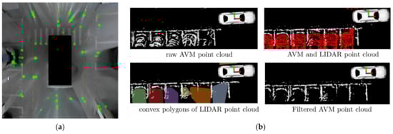
Figure 1.
Example of parking space recognition. (a) Parking space corner points detection and parking space feature extraction for automatic valet parking [2]; (b) Parking space recognition and parking lot mapping based on Lidar [3].
In parking space recognition, challenges such as complex environments, parking space diversity, sensor limitations, and computational complexity place high demands on algorithm robustness. For instance, in dynamic and complex settings, lighting conditions can vary significantly over time and with weather changes [4], leading to issues like shadows, glare, and low light at night, which can cause recognition errors or failures due to the limitations of visual sensors. Moreover, parking lots feature various parking spaces (such as parallel, perpendicular, and angled parking spaces) [5,6,7]. Therefore, parking space recognition algorithms must be capable of handling multiple types of parking spaces in real time.
In the field of parking space recognition for autonomous driving, onboard cameras have become the primary environmental perception device due to their cost advantage. Consequently, current methods for identifying and annotating parking spaces generally rely on image vision [8]. These methods include straight-line extraction for parallel and perpendicular parking spaces, corner detection for angled parking spaces, and deep learning techniques [5,6,7,9,10,11]. However, image vision is significantly affected by conditions such as heavy rain, fog, darkness, and varying light levels, which restrict its effectiveness in target recognition. In contrast, three-dimensional (3D) point cloud [12] offers significant advantages. Lidar-based 3D point cloud vision is highly resistant to interference from light sources and shadows and can provide exceptionally accurate 3D poses, delivering rich information for environmental perception. As hardware manufacturing technology advances, the cost of Lidar is expected to decrease further, potentially revitalizing environmental perception methods that rely on laser-based vision.
However, pure Lidar data has limitations in localization, particularly in complex and unknown environments, where cumulative errors can compromise its accuracy. If the integration accuracy of the IMU and Lidar is low, the resulting point cloud map may exhibit deviations that are amplified during the point cloud mapping process. This can lead to inaccurate boundary recognition of parking spaces, ultimately impacting the effectiveness of automatic annotation. The IMU (Inertial Measurement Unit) provides short-term accurate pose estimation by measuring the carrier’s acceleration and angular velocity. Still, it is susceptible to disturbances from temperature changes, vibrations, and electromagnetic fields. To overcome these challenges, tightly coupling Lidar and IMU allows for leveraging both strengths, achieving high-precision and robust automatic parking space labeling. In this approach, we integrate the IMU with Lidar’s high-precision pose detection, tightly couple the two, and use the IMU to compensate for Lidar’s pose. Based on this compensated pose, we calculate the vehicle’s Lidar odometry in unknown environments, localize and map parking scenes using the Lidar data, and ultimately achieve automatic parking space labeling.
The remaining parts of this paper are organized as follows. Section 2 reviews the literature in related fields. Section 3 describes the automatic berth marking method proposed in this paper with tightly coupled Lidar and IMU. The experiments were conducted on real-world datasets, and open datasets are discussed in Section 4. Section 5 discusses the experimental results. Finally, Section 6 summarizes the main work content of this paper.
2. Related Works
Current parking space recognition and detection methods include pure vision approaches, pure Lidar approaches, vision-Lidar fusion techniques, and IMU-coupling methods.
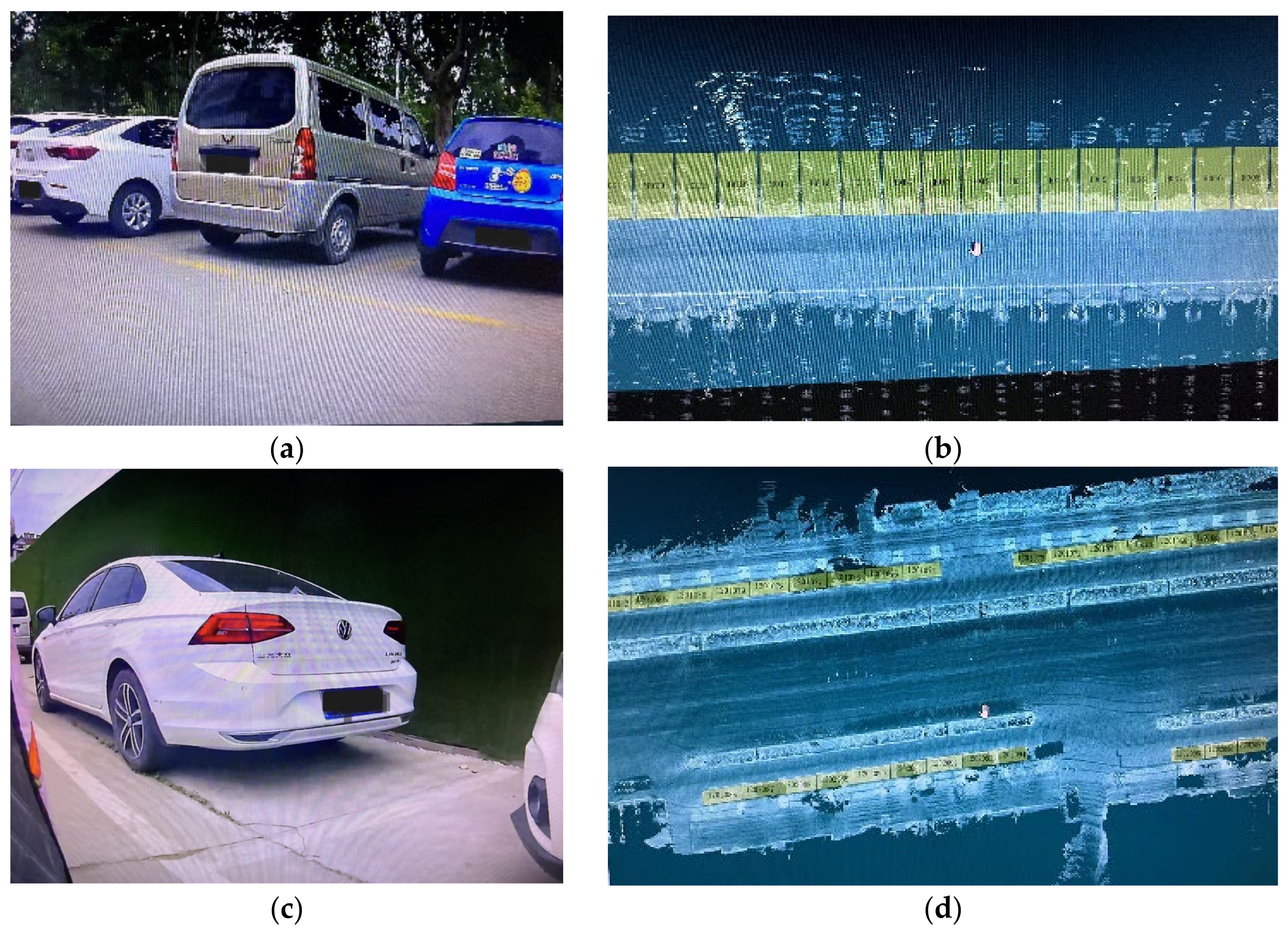
Image-based parking space detection methods face challenges such as insufficient lighting or unclear textures, leading to detection errors. As shown in Figure 2a, the texture boundary is relatively blurred at night. To address these limitations, Jiang et al. [13] introduced parking space semantic features and the concept of inverse exponential functions to improve closed-loop detection, thereby enhancing parking localization accuracy. However, localization accuracy in parking scenarios is not always closely correlated with the accuracy of parking space recognition. Deep learning-based methods can improve the accuracy of nighttime parking recognition; for example, Hasan et al. [4] developed a parking space detection method by training a deep learning network model with data from various lighting conditions. Nonetheless, they require extensive pre-training datasets, substantial training time, and significant computing power, and they incur high costs. Another approach involves image enhancement [14] to compensate for poor lighting. However, image preprocessing can alter pixel values, which may adversely affect the extraction of image features and result in only marginal improvements in parking space recognition.
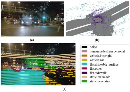
Figure 2.
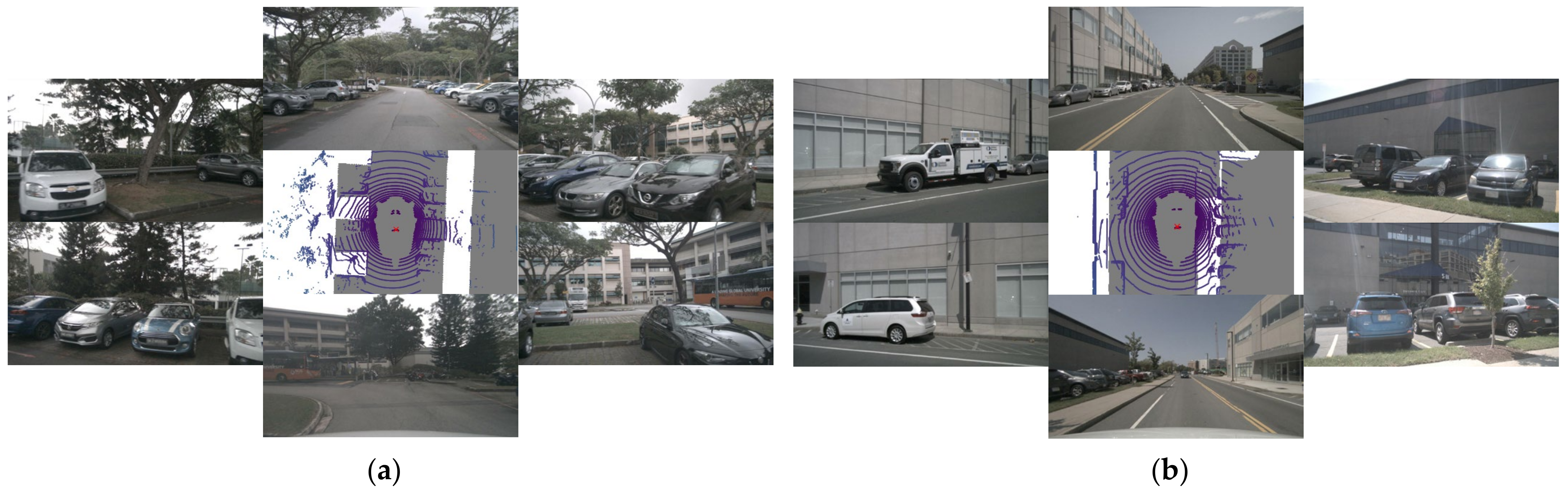
Comparison between image vision and Lidar vision, data from nuScenes [15]. (a) Image vision in a night scene; (b) Lidar vision at the same time and place; (c) Superposition of image vision and laser vision.
To address the parking challenges in scenes lacking clear or blurred lane lines under complex weather conditions, parking space detection methods based on 3D distance detection have been proposed. The Lidar-based 3D point cloud method is highly resistant to interference from light sources and shadows, providing very accurate 3D poses and rich geometric information for environmental perception, as shown in Figure 2. Figure 2b shows the bird’s-eye view (BEV) perspective of the Lidar 3D point cloud, corresponding to Figure 2a at the same time and place. Lidar detects the distance of objects using the time of flight (ToF) principle, recording their three-dimensional spatial information. The geometric structure information of the object can be derived from the 3D point cloud, which is then projected onto a two-dimensional (2D) image, as depicted in Figure 2c. In existing research, Kamiyama et al. [16] used Lidar to measure the reflection intensity of the road surface to identify white-painted parking spaces. This approach, however, is limited to scenarios with white-painted parking lines and lacks generalization across different environments. Gong et al. [17] proposed a Lidar-based parking lot localization and mapping method incorporating obstacle semantic information. While this method reduces the workload for downstream parking space annotation, it involves deep learning, making the mapping tasks labor-intensive. Jiménez et al. [18] performed parallelepiped detection to determine the occupancy status of parking spaces by analyzing the space above them. However, this method relies on prior information about the parking space location, making it unsuitable for unknown environments. Yang et al. [19] used detected 3D bounding boxes to categorize parking spaces formed by adjacent bounding boxes, calculating the minimum free space distance to determine if the space is usable for parking. Despite its effectiveness, the 3D-based method introduces an additional dimension compared to 2D methods (such as images or 2D point clouds [20]), significantly increasing computational complexity and reducing efficiency in detecting free parking spaces.
The method based on images with Lidar is another method to label parking spaces. In current image-Lidar fusion research progress, Im et al. [3] proposed a parking SLAM method utilizing vision-Lidar fusion. However, its effectiveness is limited to two standard parking scenarios—perpendicular and parallel—due to its dependency on standard storage space as a prior condition, thus limiting its generalization performance. Tong et al. [21] proposed a parking line extraction method with main orientation constraints. While this method is not restricted by the type of storage space and only relates to vehicle orientation, it is more suitable for cases where a global map is constructed. The incomplete obstacle information in a local map reduces the accuracy of vehicle orientation assessment, affecting the robustness of parking space detection. Moreover, the aforementioned vision-Lidar fusion methods rely on parking lines in image vision as prior information for detecting parking spaces. This reliance on basic prior knowledge provides a foundation for determining parking spaces. However, in some parking scenarios, clear parking space information is not provided. For instance, the modern ecological parking lot shown in Figure 3 integrates ecological concepts, making the parking lines less obvious. Consequently, vision-based or vision-fusion methods that depend on parking lines as prior information are not applicable in such scenarios. However, the above methods cannot solve the problem of high-precision scene parking detection in unknown environments. In an unknown scene lacking prior parking coordinates and visual texture information, accurately locating an autonomous vehicle and identifying parking spaces relies on the vehicle’s onboard detector to perceive the scene environment. This challenge is addressed by the SLAM method [22]. Lidar-based SLAM suffers from cumulative errors in Lidar odometry [23]. To mitigate this issue, Lidar is commonly combined with Inertial Measurement Unit (IMU) for vehicle pose estimation. The integration of Lidar and IMU extends the method’s applicability [24], offering reliable localization information even in indoor environments. The combination of Lidar and IMU can be categorized into loose coupling and tight coupling. Loose coupling involves separate Lidar-based and IMU-based estimations, fused using techniques like extended Kalman filters or factor graphs in pose estimation, ensuring high computational efficiency [25]. In contrast, tightly coupled Lidar and pre-integration IMU is integrated into a unified objective function during front-end measurement. This approach robustly estimates sensor trajectories in environments with fewer features, achieving high-precision localization and mapping [26], crucial for robust automatic parking space recognition. Leading tightly coupled Lidar-IMU odometry methods include LIO-SAM [27], LIC-Fusion [28], Super Odometry [29], LVI-SAM [30], FAST-LIO [31], and LILO [32], widely used in current applications.
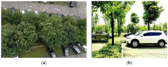
Figure 3.
Modern ecological parking lots where parking lines cannot be detected. (a) Top-view image of a parking lot; (b) Image of an ecological parking lot.
In point cloud SLAM, the point cloud registration process is crucial. Point cloud registration encompasses both traditional ICP (Iterative Closest Point) and its improved variants and registration methods based on deep learning techniques. The ICP algorithm [33] is one of the most classic methods for point cloud registration. Its fundamental approach minimizes the distance error between the source and target point clouds through iterative optimization. Various improvements to the ICP algorithm have been developed to address specific application scenarios, including GICP (Generalized ICP) [34], NDT (Normal Distributions Transform) [35], and so on. With the advancement of deep learning technology, these methods leverage deep learning to handle noise, occlusion, and complex scenes by learning point cloud data feature representations. For instance, PointNetLK [36] utilizes PointNet for point cloud registration tasks and has shown promising results. DeepGMR (Deep Gaussian Mixture Model RANSAC) [37] combines deep learning feature extraction with the RANSAC algorithm to improve registration accuracy and robustness in noisy point cloud data. Despite these advances, deep learning-based registration methods typically require extensive data annotation and model training. In contrast, the ICP method does not rely on extensive training datasets, making it more adaptable to smaller or less annotated datasets. The ICP algorithm is simple and easy to implement and understand. It performs well, especially when dealing with dense point clouds and good initial alignments, allowing for rapid convergence. It also has lower computational overhead and is relatively more straightforward to implement. Given these factors, this article employs the ICP method for point cloud registration.
In summary, parking space recognition, also referred to as free space detection, encounters numerous challenges. Firstly, the parking space detection method based on images struggles to maintain effectiveness in complex, unknown environments. Secondly, the pure Lidar-based parking space detection method cannot ensure the accuracy and complexity of mapping and parking space recognition in the AVP system.
Therefore, we proposed an automatic parking space recognition approach that tightly couples Lidar with IMU based on the geometric relationship between the vehicle and the parking space, leveraging accurate 3D pose information from point clouds. The IMU compensates for Lidar pose, enabling precise vehicle localization, local map construction of unknown parking scenes, and identification of vacant parking spaces. This approach enhances the robustness of parking space recognition and annotation. Compared to existing methods, our approach offers the following contributions:
- We propose a parking space detection method based on tightly coupled Lidar and pre-integrated IMU. By integrating Lidar point clouds with IMU data tightly, we construct a high-precision localization and grid map. This method identifies free space between obstacle vehicles using convex hull detection and the Hough transform on the grid map, and finally determines parking spaces based on vehicle size constraints. Therefore, our method achieves high-precision perception of parking scenes.
- We rely solely on Lidar for perceiving the parking scene, eliminating the need for prior maps or parking space information at the input data source. In contrast to current Lidar parking space detection methods that rely on prior information from maps or images, our approach enables precise parking space detection in unknown and complex environments.
- We propose a polarized Lidar matrix transformation method in Lidar SLAM. Our approach converts 3D point clouds into 2D matrices and integrates BEV projections of point cloud grid maps to achieve parking space recognition. By compressing 3D data into 2D, we reduce data storage requirements without sacrificing critical features, thereby addressing the high complexity associated with 3D point cloud processing.
3. Methodology
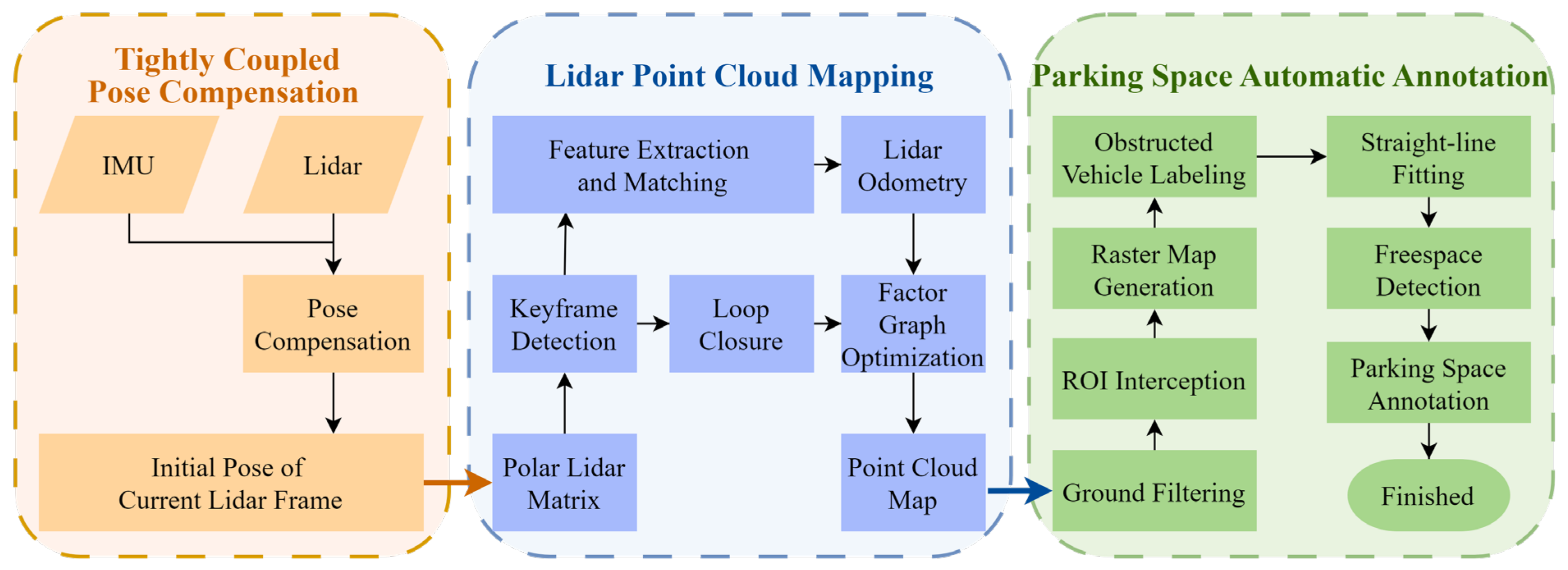
The method proposed in this paper is illustrated in Figure 4 and consists of three main components: tightly coupled pose compensation, Lidar point cloud mapping, and parking space automatic annotation. First, the collected Lidar data is combined with IMU data for pose compensation. Next, the Lidar odometry and keyframes are calculated to provide initial values for the compensated pose, constructing a three-dimensional point cloud map of the parking scene based on the polarized Lidar odometry and historical keyframes. Finally, the regions of interest (ROI) after filtering out the ground points are extracted from the three-dimensional point cloud map to generate a grid map. This grid map is then used to identify obstacle vehicles, detect free spaces, and mark available parking spaces.
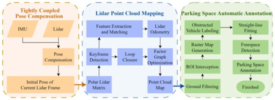
Figure 4.
Flow chart of parking space automatic recognition method.
The symbols and variables involved in this paper are defined in Table 1.

Table 1.
Definition of symbols and variables.
3.1. Tightly Coupled Pose Compensation
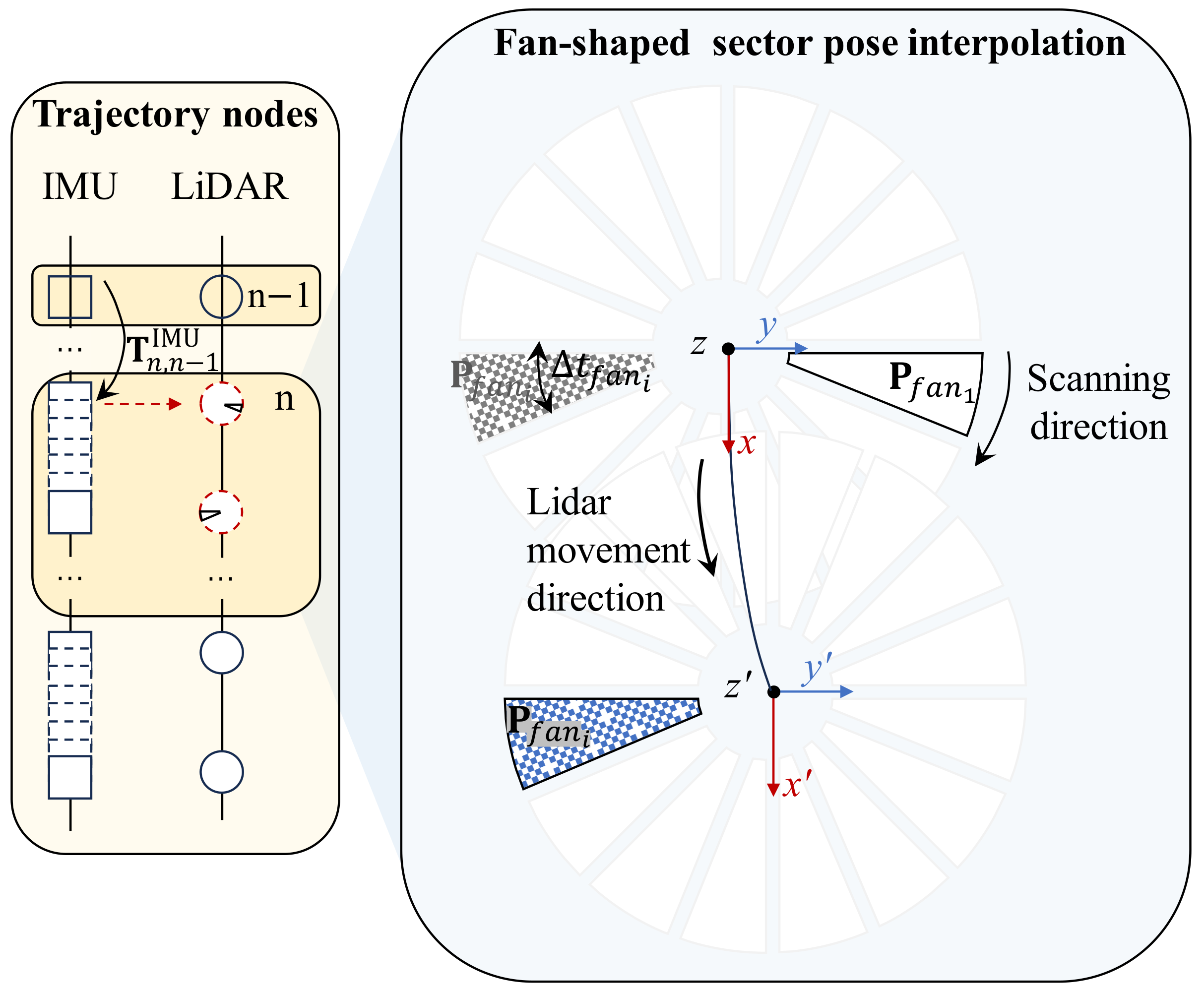
Mechanical Lidar detects the environment by rotating the laser emitter during data collection. Data is generally collected and stored in the form of equal-angle fan-shaped sectors starting from the Y axis in a clockwise direction. For example, each laser frame contains 75 equal-angle fan-shaped sectors. The acquisition time for each fan-shaped sector in a Lidar frame with an operating frequency of 10 Hz is 1.33 ms. However, during movement, the vehicle carries the mounted Lidar along with it, resulting in an additional superimposed change in the Lidar’s movement direction besides the change in the scanning direction between the various fan angles in the laser scanning frame. As shown in Figure 5, after the superposition change of the scanning and movement directions, the fan angle is transformed into in the ego body coordinate system. IMU can output high-frequency pose data through dead reckoning (DR). Therefore, the pose-transformation matrix between adjacent Lidar frame nodes can be calculated by coupling the pose information output by IMU pre-integration [38]. The fan-shaped sector can then be compensated for pose using a timestamp-based linear interpolation method. The initial pose value of the current laser frame can be estimated by combining the pose of the previous laser historical keyframe.
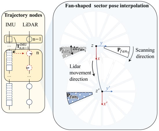
Figure 5.
Schematic diagram illustrating posture compensation with tightly coupled Lidar and IMU.
In Figure 5’s trajectory nodes’ queue, represents the current laser frame, and the pose of the th laser historical key frame is obtained from Section 3.2. denotes the rotation matrix of the pose relative to the origin coordinate, and represents the translation vector. This section focuses on standardizing the pose of the current th laser frame, which includes calculating the reference pose of the current laser frame and compensating for the fan-shaped sector pose based on this reference pose of laser frame.
First, the reference pose of the current laser frame is calculated. This reference pose is obtained through IMU coupling. IMU pre-integration [27] outputs the pose-transformation matrix from the adjacent node to :
Among these variables, represents the vehicle speed, and denotes the acceleration due to gravity. Then, the initial posture of the current laser frame can be determined using the IMU posture transformation formula:
where is obtained from Section 3.2; represents the external parameter relationship between IMU and Lidar.
Secondly, perform posture compensation on the fan-shaped sector of the current laser frame. Posture compensation corrects the offset caused by the movement of the ego vehicle during a laser scan, aligning all fan-shaped sectors’ coordinate systems within a frame to the coordinate system of the first fan sector. The timestamp of the first fan sector in the current frame serves as the calibration timestamp, establishing the body coordinate system for the entire laser panoramic frame. The posture transformation between the first fan angle and the th fan angle is calculated using the timestamp linear interpolation method:
Solve the pose-transformation relationship between the two coordinate systems of the th fan-shaped sector and the first fan-shaped sector:
Then, according to the coordinate mapping, the position and posture of the th fan-shaped sector laser data are mapped to the coordinate system of the first fan-shaped sector:
Based on the above formula, the data of each fan-shaped sector can be reassembled into a complete unbiased panoramic surround laser frame to complete the posture compensation of the current laser frame .
3.2. Lidar Point Cloud Mapping
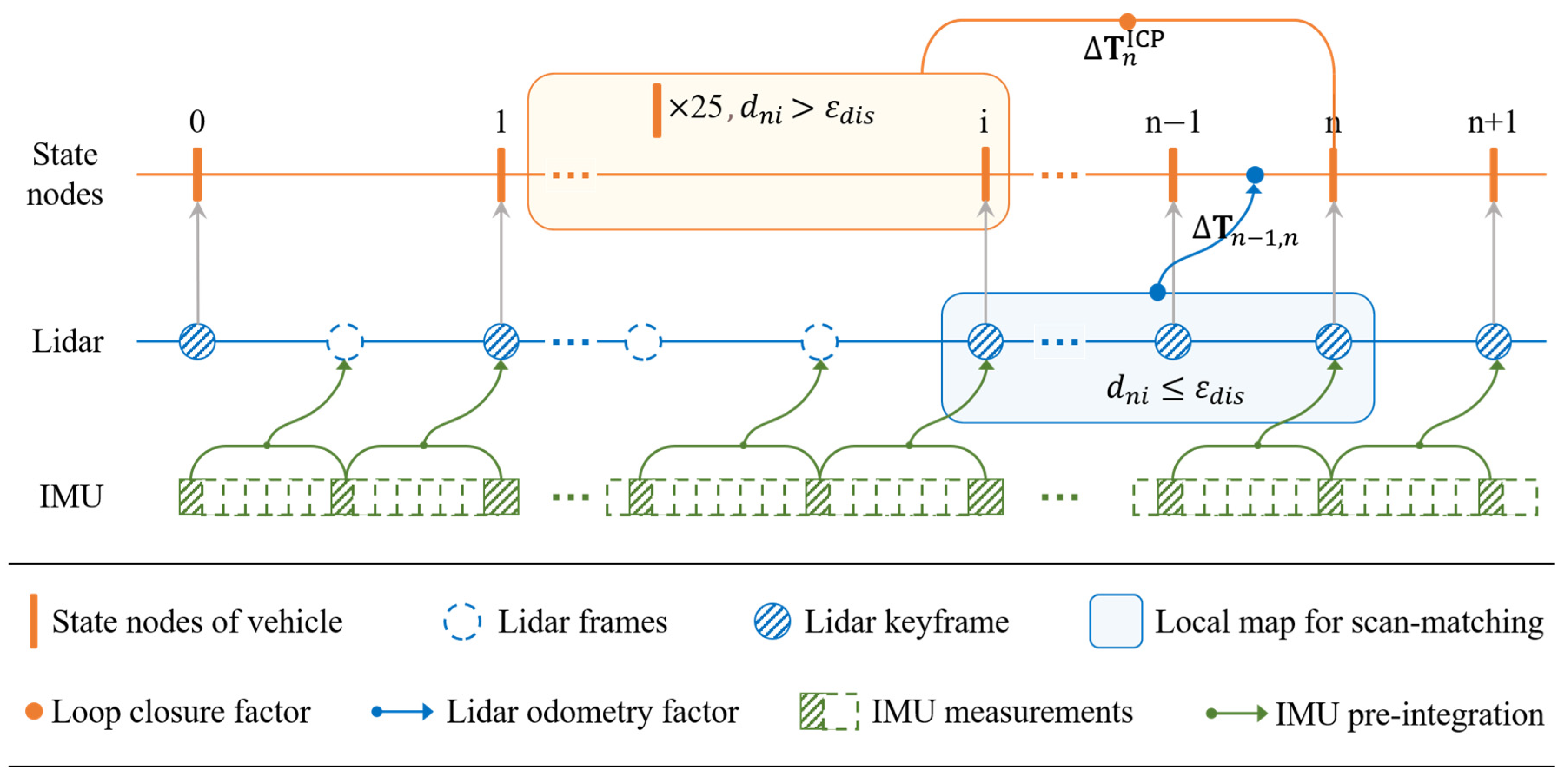
Constructing an accurate scene map based on tightly coupled pose-compensated Lidar data is fundamental and crucial for parking slots identification and annotation. In this section, the initial pose value is integrated with the polarized matrix of point cloud to compute the front-end Lidar odometry. Subsequently, the polarized Lidar odometry and loop detection are incorporated as factors into the iSAM2 graph optimizer [39]. As depicted in Figure 6, the green squares denote the IMU sequence data, the blue circles represent the Lidar sequence data, and the orange bars indicate the vehicle pose state nodes. First, as illustrated in Section 3.1, the IMU data between Lidar frames is pre-integrated, as indicated by the green arrow, to compensate for the Lidar frame pose, resulting in the compensated Lidar frame pose . The subsequent content of this section elaborates on this process. Secondly, polarization matrix conversion and keyframe extraction are performed on these compensated Lidar frames. The order of these steps can be interchanged; for instance, polarization matrix conversion can be applied to each frame before extracting keyframes, or keyframes can be extracted first, followed by calculating the polarization matrix for the selected frames. Lines within circles represent the extracted Lidar keyframes. In the third step, Lidar odometry is calculated from the extracted polarized features of the keyframes, generating state nodes in the Lidar odometry series. Specifically, polarized edge and planar features are computed for the extracted keyframes, and scan-matching is performed to establish the keyframe state nodes, which are represented by the orange elements in Figure 6. Finally, in those state nodes, the polarized Lidar odometry factor and loop closure factor , constrained by the distance threshold , are all sent into iSAM2 to construct a point cloud map. This process achieves optimization for smoothing the Lidar poses, followed by mapping the pose data from all historical keyframes to the global coordinate system for reconstruction, thereby generating the 3D point cloud map of the parking scene.

Figure 6.
Schematic diagram of polarized Lidar odometry and loop closure.
3.2.1. Polarized Lidar Odometry Factor
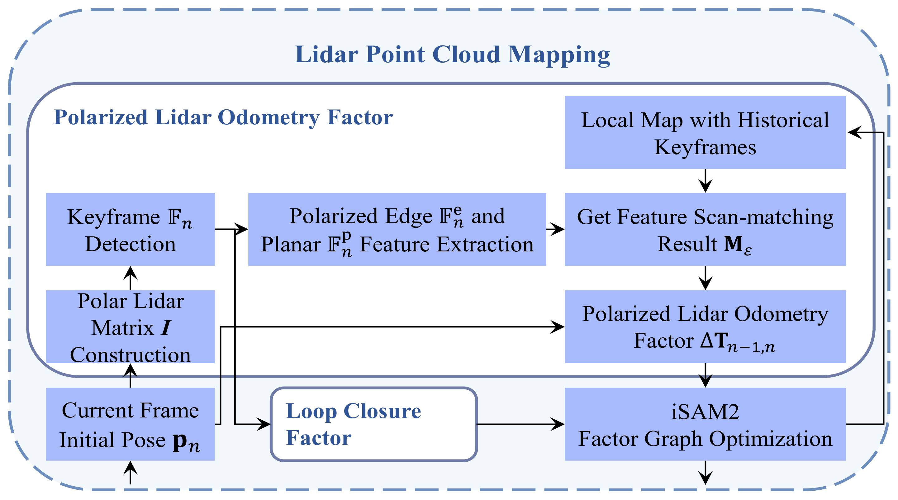
Since the coordinate system of the first fan-shaped sector serves as the reference body system in posture compensation, the resultant posture calculated by the posture transformation matrix for the panoramic laser frame represents the initial posture value of the current frame, denoted as . The polarized odometry calculation for the current frame involves polarized feature extraction and nearest node matching. As shown in Figure 7, initially, the point cloud polar coordinates are computed and mapped into a two-dimensional polarized matrix. At the same time, the keyframes are extracted. Subsequently, the polarized edge features and polarized planar features are derived from this matrix. By matching the point cloud polarized features of the current frame with the local map, in conjunction with the initial posture value, the posture of the current Lidar frame is determined.

Figure 7.
Flow chart of polarized Lidar odometry.
- Polar Lidar Matrix Construction
The number of point clouds in one frame is extensive, necessitating the construction of a point cloud polarized matrix based on Lidar operating parameters to polarize the Lidar frame in two dimensions. The corresponding relationship between the polarized matrix and a point in the Lidar frame is as follows:
where denotes the mapping between the vertical angle of the point cloud and the row index, determined by the vertical angle distribution specific to different Lidar models. For instance, in the case of a 16-line Lidar with a horizontal angular resolution of 0.2°, there are 16 scanning lines and 1800 columns in the matrix. The row index in the two-dimensional matrix is calculated based on the laser line ID to which the point cloud belongs, while the column index is determined by the horizontal azimuth angle of the point cloud using the formula . The depth value in the matrix represents the Euclidean distance from the point cloud to the Lidar coordinate system. This construction method results in a two-dimensional matrix known as the polarized matrix of point cloud. It should be noted that when the polarized matrix is expanded into a three-dimensional tensor, each element can store multiple channel values, such as point depth and intensity.
- 2.
- Keyframe Detection
Feature extraction and matching across all frame nodes are time-consuming and resource-intensive, necessitating keyframe extraction. The method involves calculating the pose transformation between the current laser frame and the previous laser historical keyframe to determine if the current frame qualifies as a keyframe. This calculation includes determining the roll angle transformation , pitch angle transformation , yaw angle transformation , and translation transformation between the current laser frame and the previous historical keyframe . When any of these transformations exceed their respective thresholds, the current laser frame is designated as a keyframe. The newly identified keyframe is linked to the new vehicle state node in the factor graph, and all Lidar frames between the two keyframes are discarded. In our approach, the roll angle transformation threshold , pitch angle transformation threshold , yaw angle transformation threshold , and translation transformation threshold are predefined.
- 3.
- Feature Extraction
The feature description of the polarized matrix uses the method of extracting polarized edge features and polarized planar features. The curvature of each point cloud is calculated based on the polarized matrix, and the edge and planar feature points are screened out. Select an equal number of matrix points on both sides of the point cloud , which must be in the same matrix row as the point, and calculate the curvature of the point cloud according to the point cloud curvature calculation formula [40,41]:
where when the is greater than the edge feature point curvature threshold , the point is an edge feature point; when it is less than or equal to the planar feature point curvature threshold , the point is a surface feature point. The edge feature point curvature threshold is and the surface feature point curvature threshold is in our method.
- 4.
- Feature scan-matching
The scan-matching of the nearest node uses the L-M algorithm. Based on the initial pose value, the feature point cloud in the current laser frame is mapped to the global coordinate system. Historical keyframes with a Euclidean distance to the current laser frame less than or equal to the Euclidean distance threshold are selected, i.e., . The feature point cloud of these historical keyframes is then mapped to the global coordinate system according to their poses to obtain the local map :
where represents the Euclidean distance between the th frame and the th frame of Lidar. In our method, the Euclidean distance threshold is .
The point-line matching method is used for matching edge feature points. The point cloud is regarded as an edge feature point in the current laser frame, and the nearest five edge feature points are found in the local map. If these five edge feature points can be fitted into a straight line, the match is successful, and these successfully matched edge feature points are retained. The point-surface matching method is used for matching planar feature points. The point cloud is regarded as a planar feature point in the current laser frame, and the nearest five planar feature points are found on the local map. If these five planar feature points can be fitted into a plane, the match is successful, and these successfully matched planar feature points are retained. Solve the current laser frame pose based on the L-M algorithm and the matched feature points:
where and represent the sequence numbers of the feature points in the corresponding features.
3.2.2. Loop Closure Factor
This section constructs a point cloud map using the poses of historical laser keyframes and registers features with the current laser frame. Firstly, as illustrated in Figure 8, it identifies 25 consecutive historical keyframes [27] with a Euclidean distance greater than from the current laser frame , mapping their feature point clouds to the global coordinate system based on corresponding poses to establish the historical map. Secondly, it maps the feature point cloud of the current laser frame to the global coordinate system using the solved pose, and registers this with the historical map using the ICP method.
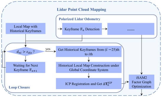
Figure 8.
Flow chart of loop closure.
The relative transformation obtained from the above registration serves as the loop closure factor. This factor, along with the polarized Lidar odometry factor, is input into the iSAM2 factor graph optimization to refine the final pose state of the current th frame. This refined pose state represents the result after correction based on the historical map.
3.3. Parking Space Automatic Annotation
After constructing the Lidar point cloud map of the parking scene, meticulous calculations and continuous optimization of localization and mapping modules have enabled us to build a high-precision environmental map and achieve an accurate ego pose. This stage establishes a solid foundation for the vehicle’s parking-detection task in unfamiliar environments. During the parking-detection phase, ground point cloud and elevation information minimally affect the accuracy of parking detection. Therefore, the map undergoes initial filtering and grid to mitigate redundant information, obtaining grid data on obstacle vehicles within parking spaces. Subsequently, the straight-line fitting of the vehicle body’s top-down projection are used to fit point cloud straight lines. Free parking spaces are then calculated by combining these fitted lines with constraints based on vehicle body size, ultimately marking available parking spaces.
3.3.1. Ground Point Segmentation and Grid Map Construction
Lidar point cloud mapping generates a 3D map containing ground point cloud and elevation data. In order to reduce the impact of redundant ground point data and elevation data on parking space detection and accurately identify obstacle vehicles, the ground points need to be segmented and filtered first, and then BEV projection is performed to construct a grid map.
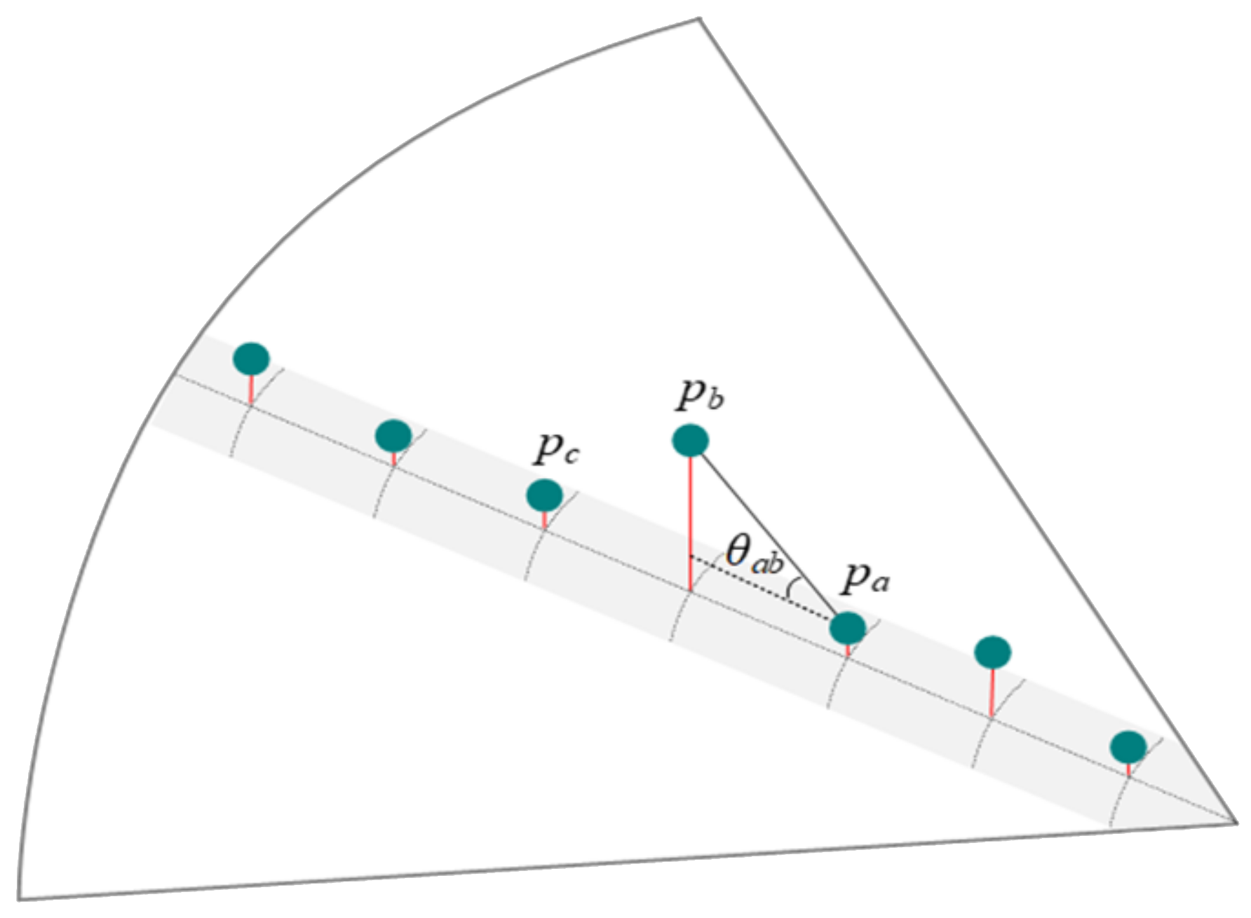
The ground point segmentation adopts the vertical angle evaluation method [42]. Figure 9 is a schematic diagram of the vertical angle evaluation method. The point strip is a point cloud in the same horizontal orientation (i.e., on the same vertical plane, with the same ) in a single-frame point cloud. The vertical angles between the point clouds are calculated in order from small to large according to the point cloud depth , and compared with the vertical angle threshold to determine the ground points, thereby eliminating the ground points. Based on the above method, all ground points in a single-frame point cloud can be eliminated. The ground-filtering process is in frames. When all the lasers included in the point cloud map have completed the ground-filtering process, the remaining point cloud is the required point cloud. For example, in Figure 9, it is assumed that is the determined ground point cloud, and are the laser point clouds to be determined, and the vertical angle threshold is . Connect point clouds and , and calculate the vertical angle of the point cloud connecting line :
where if is less than , then belongs to the ground point. Connect points and , and use the above method to determine whether belongs to the ground point; if is greater than , then does not belong to the ground point. Connect points and , and use the above method to determine whether belongs to the ground point.
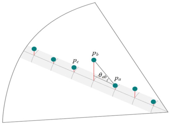
Figure 9.
Schematic diagram of the vertical angle evaluation method.
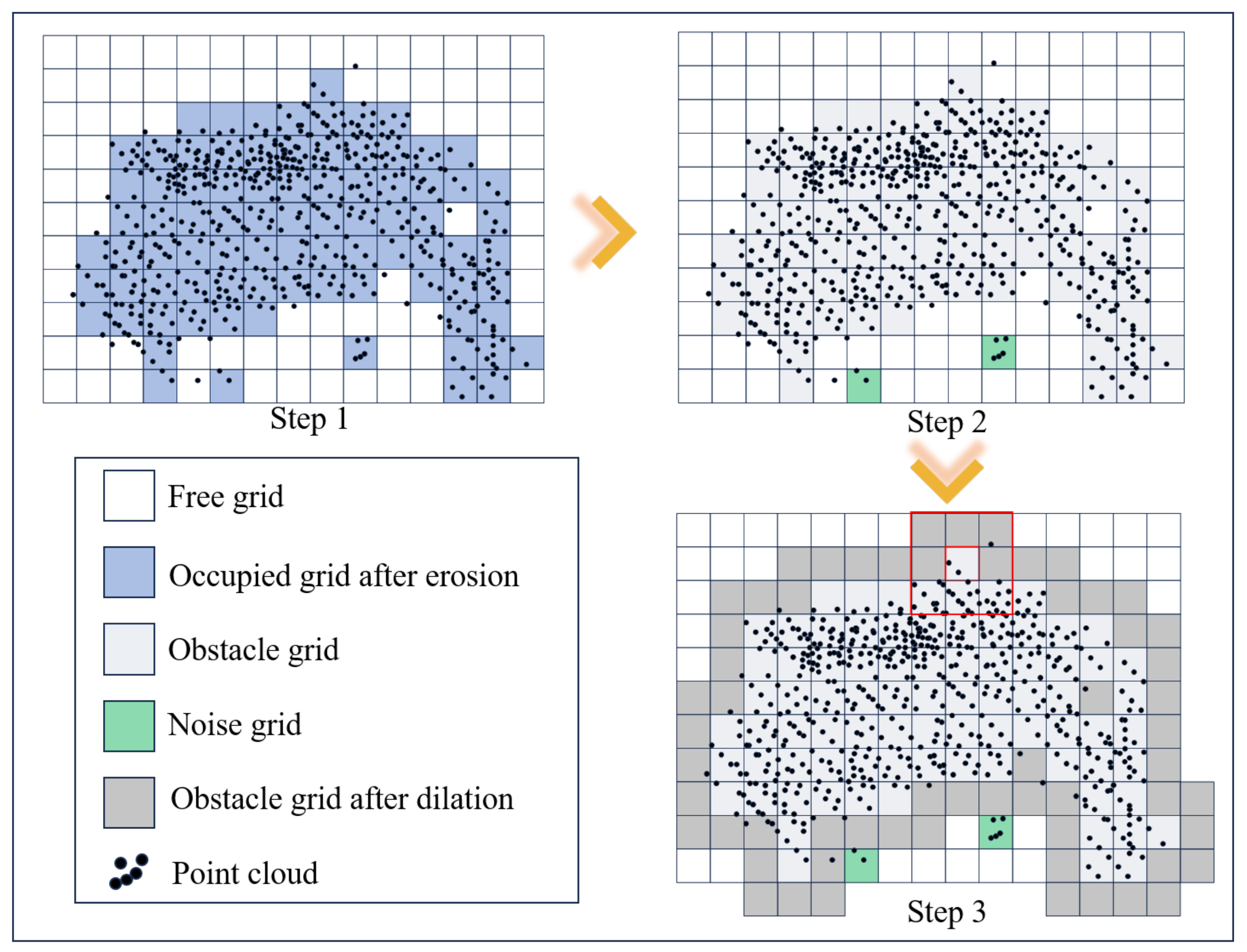
For the scene map with ground point clouds filtered out, it is necessary to extract the ROI and construct a BEV grid map based on the ROI, using erosion and dilation algorithms to mark obstacle grids. The bounding box of the ROI is set according to the actual scene dimensions, . The ROI is extracted from the point cloud map and projected into a BEV grid map with a scale of and . In the grid map, as shown in Figure 10: the first step is, if the point cloud density in a single grid is not less than two, the grid is marked as occupied; otherwise, it is marked as free. To further refine this map, erosion removes small clusters of noise or isolated points that may falsely indicate occupancy. This step ensures that the occupied grids more accurately represent significant obstacles or structures in the environment, thereby improving the overall reliability of the map. The second step is, traverse the occupied grids and check the status of their eight surrounding grids. If at least one of the surrounding grids is also occupied, the grid is marked as an obstacle; otherwise, it is marked as noise. The third step is, traverse all obstacle grids and mark the eight surrounding grids as obstacles.
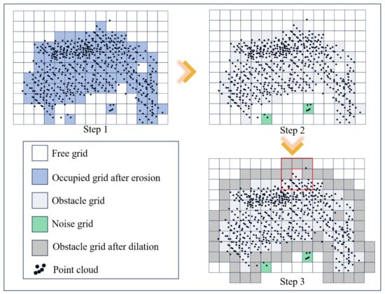
Figure 10.
Schematic diagram of the barrier grid marking method based on erosion and dilation.
3.3.2. Obstacle Vehicle Detection and Vacancy Annotation
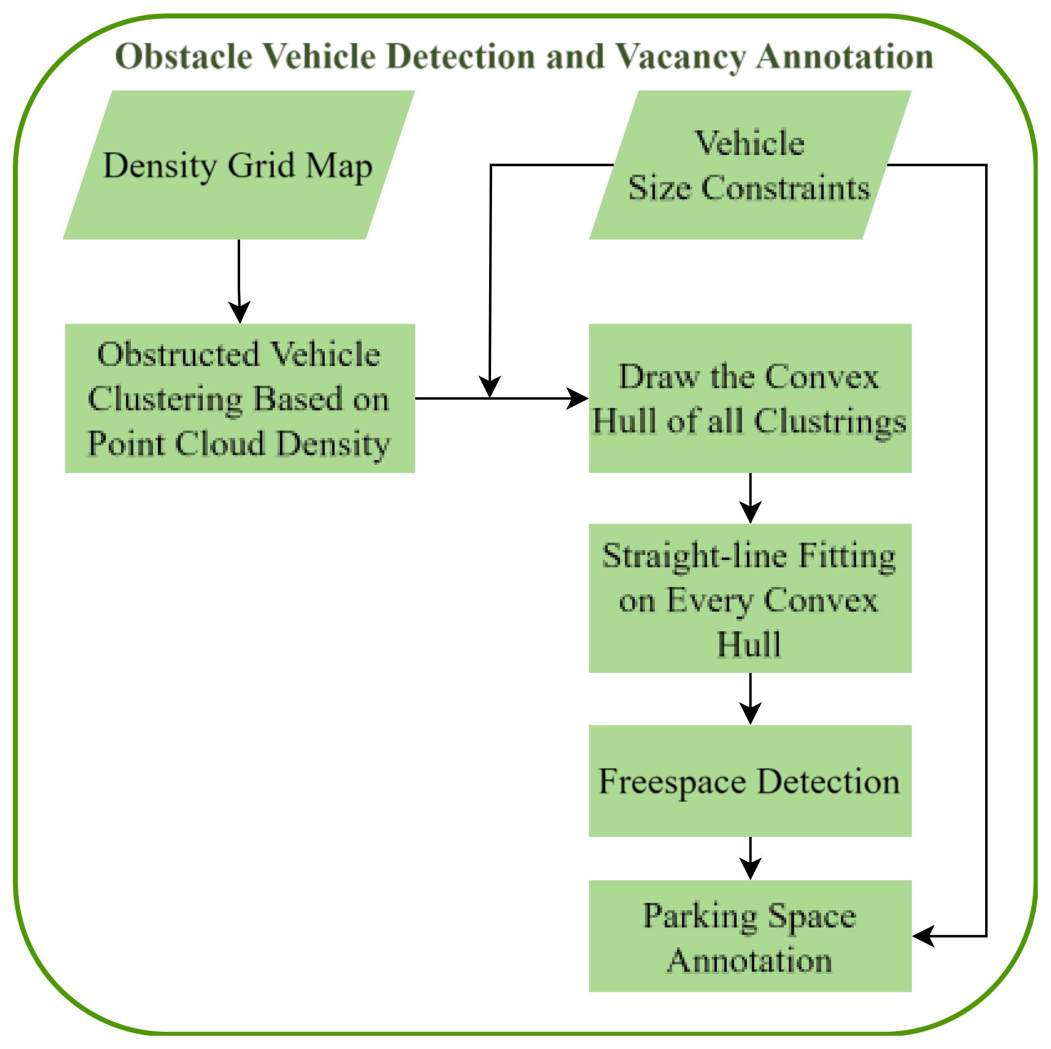
The implementation of obstacle vehicle detection and vacancy annotation based on fitted lines requires the extraction of vehicle contours from the point cloud. In this section, the extraction of vehicle contours is performed on the obstacle grid map after erosion and dilation. The specific method in Figure 11 is as follows: first, use the grid occupancy point density information to cluster the point cloud, retaining vehicle point clouds based on vehicle size constraints; next, draw a convex hull on the retained vehicle point clouds and fit the vehicle contour lines on the convex hull; finally, use the fitted lines as prior information combined with vehicle size constraints to mark vacant parking spaces. We categorize parking spaces into three types based on the parking method: perpendicular parking spaces, angled parking spaces, and parallel parking spaces, as shown in Figure 12. The method described in this section is applicable to all three types of parking spaces.

Figure 11.
Flow chart of obstacle vehicle detection and vacancy annotation.
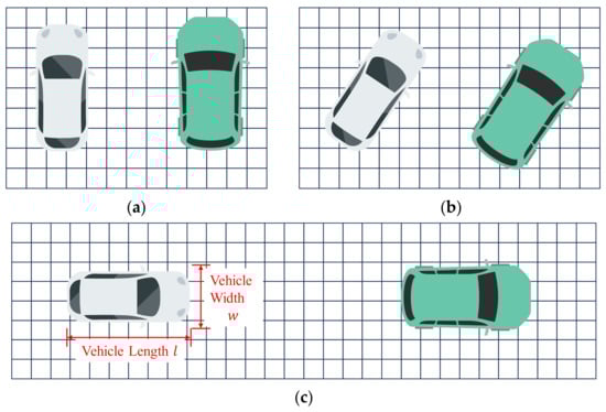
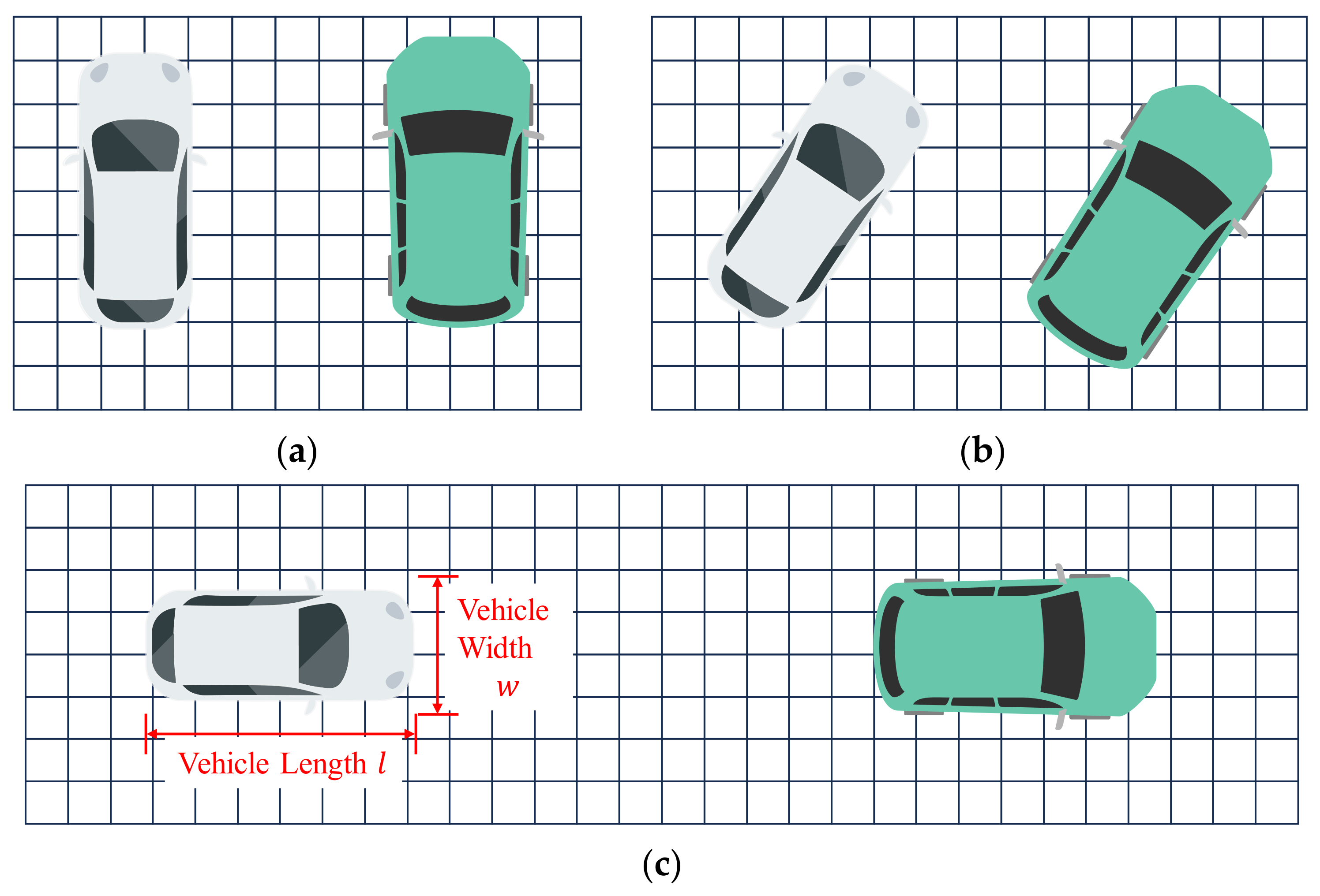
Figure 12.
Parking slots classification (based on grid projection). (a) Perpendicular parking space; (b) Angled parking space; (c) Parallel parking space.
The grids in the obstacle grid map contain occupancy point density information. Based on this density, the DBSCAN algorithm is used to cluster the obstacle points on the planar grid, resulting in different point cloud clusters . The DBSCAN effectively handles noise points and outliers, does not require predefined numbers of clusters, and is robust to varying cluster shapes. The DBSCAN algorithm uses a neighborhood sample count threshold of and a neighborhood distance threshold of . To more accurately filter out vehicle point clouds, vehicle size is used as prior information:
where in our method, , .
Based on the Graham algorithm, the convex hull is drawn for the retained obstacle clustering targets to achieve obstacle recognition. The obstacle convex hull satisfies:
The vehicle contour straight line is fitted using Hough transform on the grayscale image. Therefore, a density grayscale image is first generated based on the obstacle grid image. The grid grayscale calculation formula is:
where is the point cloud density value in the current grid and is the maximum point cloud density value of the entire grid map.
The obstacle boundary is intercepted in the generated grayscale image, and the boundary straight line is extracted based on the Hough transform with the following conditions as the convergence conditions:
where represents the point cloud density outside the extracted boundary line and represents the point cloud density inside the extracted boundary line. denotes the length of the long side of the extracted line for perpendicular or angled parking slots, while denotes the width of the extracted line for parallel parking slots. Specifically, if the point cloud density outside the extracted boundary line is significantly lower than inside, and the difference between the length of the extracted line and the prior size of the obstacle boundary is within a certain threshold range, then the extracted line is identified as the boundary straight line of the obstacle. If these convergence conditions are not met, the extracted straight line is treated as a boundary range, and the fitted straight line is used as prior information for the next boundary straight-line fitting process. Subsequent boundary extraction will be based on this range.
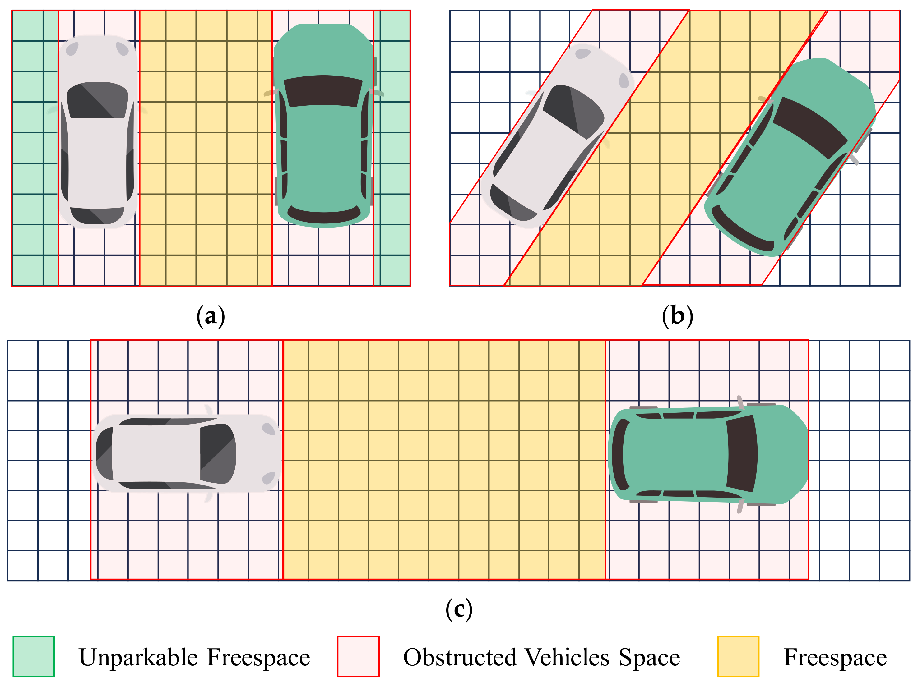
After the obstacle boundary extraction is completed, the boundaries of adjacent obstacles form a free space, as shown Figure 13. Calculate the coverage of the free space. If the coverage can envelop one or more parking spaces, that is, the size of the free space is proportional to the length or the width , then mark it as a free parking space:
where represents the length of the free space of the parallel parking slots; represents the width of the free space of the perpendicular.
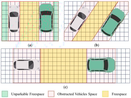
Figure 13.
Diagram of parking space recognition and annotation. (a) Annotation diagram of perpendicular parking space; (b) Annotation diagram of angled parking space; (c) Annotation diagram of parallel parking space.
During the driving process, it is important to note that the vehicle body and the parking space (occupied by another vehicle) are not always perpendicular to each other. In our algorithm, we have incorporated a technique: upon extracting the first straight line, we calculate its relative coordinates. Subsequent straight lines are then transformed into the coordinate system of this first straight line. Additionally, angled parking spaces are handled similarly to parallel and perpendicular spaces in reality. For angled parking spaces, the process involves rotating and translating the vehicle and other vehicle point clouds into the coordinate system of the first extracted straight line. We then calculate and compare it with .
4. Experiments
4.1. Experimental Environments
The experiment was conducted on a personal computer using both local dataset and open dataset. The local dataset is detailed in Section 4.1.1, and the open dataset is described in Section 4.1.2. The personal computer used for the experiment is equipped with a 1.70 GHz 12th Gen Intel(R) Core (TM) i7-1255U processor, 16GB RAM, and an RTX 2050 GPU. The algorithm proposed in this paper, along with the comparison algorithm, was implemented in a single thread within a Python environment. For the comparison literature involving deep learning algorithms, we obtained the pre-trained parameters and reproduced the code accordingly.
4.1.1. Local Datasets
The experimental local dataset was collected from various roadside parking strips and parking lots in two cities in China. The number of parking spaces in the dataset is detailed in Table 2. These parking spaces include parallel, perpendicular, and angled configurations. To increase the sample size, two field experiments were conducted at Site 1. Due to different planning batches and standards, the parking spaces do not have uniform sizes. The ground truth of the parking spaces was obtained through manual surveys and comparisons. Figure 14 shows the local experiment pictures of various types of parking spaces along with the manual annotation results for different parking space types.
Table 2.
Parking space statistics.

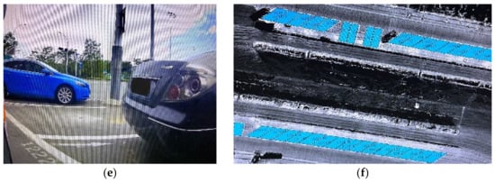
Figure 14.
Schematic diagram of parking slot types and actual arrangements in local data. (a) Perpendicular parking slots; (b) Arrangement of perpendicular parking slots; (c) Parallel parking slots; (d) Arrangement of parallel parking slots; (e) Angled parking slots; (f) Arrangement of angled parking slots.
The test vehicle is equipped with Lidar and IMU equipment. The Lidar beam has 16 lines, an operating frequency of 10 Hz, a horizontal angular resolution of 0.2°, and can sense the surrounding environment within a range of 0.5 m to 150 m in 360°. The IMU can output high-frequency posture data at 50 Hz. The size threshold of the experimental vehicle is 2 m × 4 m. The details of device parameters for the local dataset used are shown in Table 3.
Table 3.
Comparison of Lidar and IMU parameters between the local test vehicle and the open- dataset test vehicle.
4.1.2. Open Datasets
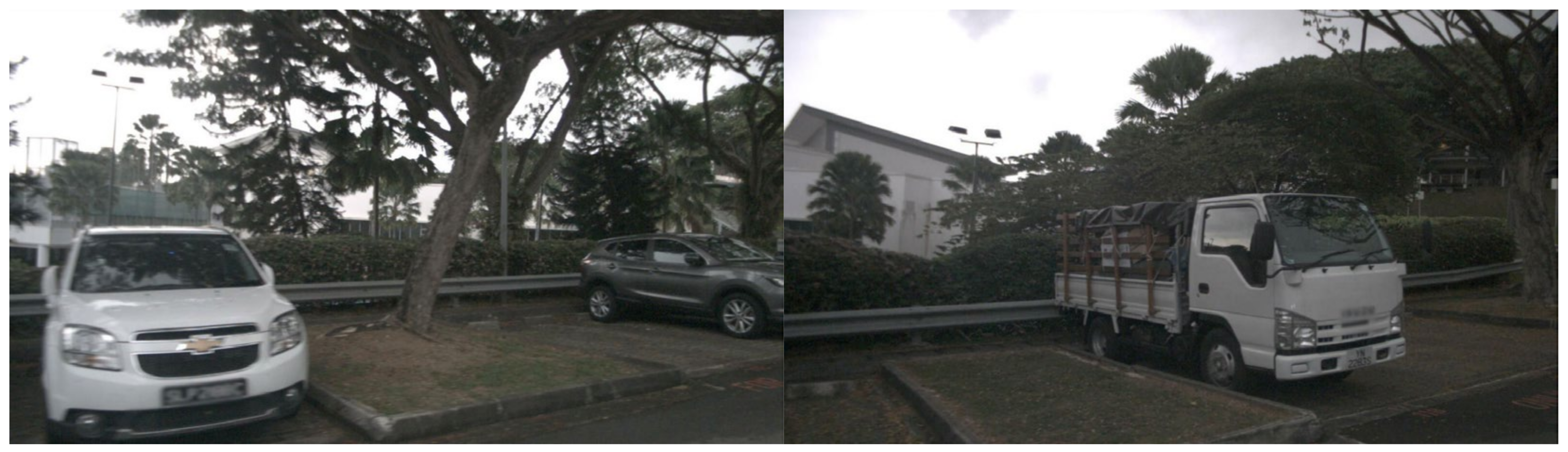
The comparative experiment is based on the open dataset nuScenes [15], which contains urban road scene perception data from IMUs, cameras, and Lidars. To evaluate the effectiveness of our proposed algorithm, we extracted parking lot and on-street parking data from this dataset for testing. The ground truth number of parking spaces in the dataset is shown in Table 4. Since the dataset does not specifically focus on collecting parking lot data, and the data is collected while the vehicle is in motion, we count the number of parking slots based on the point cloud projection occupying more than 50% of the vehicle projection area. Parked cars and parking spaces far from the driving direction are not included in the ground truth. For instance, taking the parking lot in Singapore’s Queenstown as an example, the garages in the dataset are in the form of perpendicular parking spaces, as shown in Figure 15a. For parallel parking spaces, consider a section of Boston Seaport, as shown in Figure 15b. These data were collected while the vehicle was in motion, allowing for motion estimation, SLAM mapping, and parking space detection based on these data. This meets the computational requirements of both our algorithm and the comparative algorithm. It should be noted that there is no angled parking data in this dataset. However, from the perspective of coordinate transformation, the difference between angled parking and perpendicular parking is merely a rotation angle. Therefore, detecting angled parking involves transforming the coordinates of the fitting straight line representing the angled parking to align with the perpendicular parking scene. Consequently, the experiment on perpendicular parking can represent the detection results of angled parking, as Section 3.3.2 illustrated.
Table 4.
Parking space statistics of nuScenes.
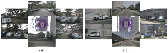
Figure 15.
Examples of parking scenes in nuScenes [15]. (a) A parking lot in Queenstown, Singapore; (b) A on-street parking area at Boston Seaport.
The hardware used to collect data in the open dataset nuScenes includes a Lidar, an IMU, and six surround-view cameras. The Lidar system has 32 lines, an operating frequency of 20 Hz, a 360° horizontal FOV, a −30° to 10° vertical FOV, a detection range of 70 m, a detection accuracy of 2 cm, and captures 1.4 million point clouds per second. The IMU outputs high-frequency pose data at 100 Hz. The resolution of the six surround-view cameras is 1600 × 900, compressed in JPEG format, with a sampling frequency of 12 Hz. The nuScenes experimental vehicle is a Renault Zoe mini electric car, measuring 3.45 m in length, 1.68 m in width, and 1.42 m in height. Considering the safety distance, the size threshold of the vehicle in x-y plane is set to 2 m × 4 m. The comparison of device parameters between the local and open datasets used is presented in Table 3.
4.2. Performance Evaluation
4.2.1. Verification Experiment
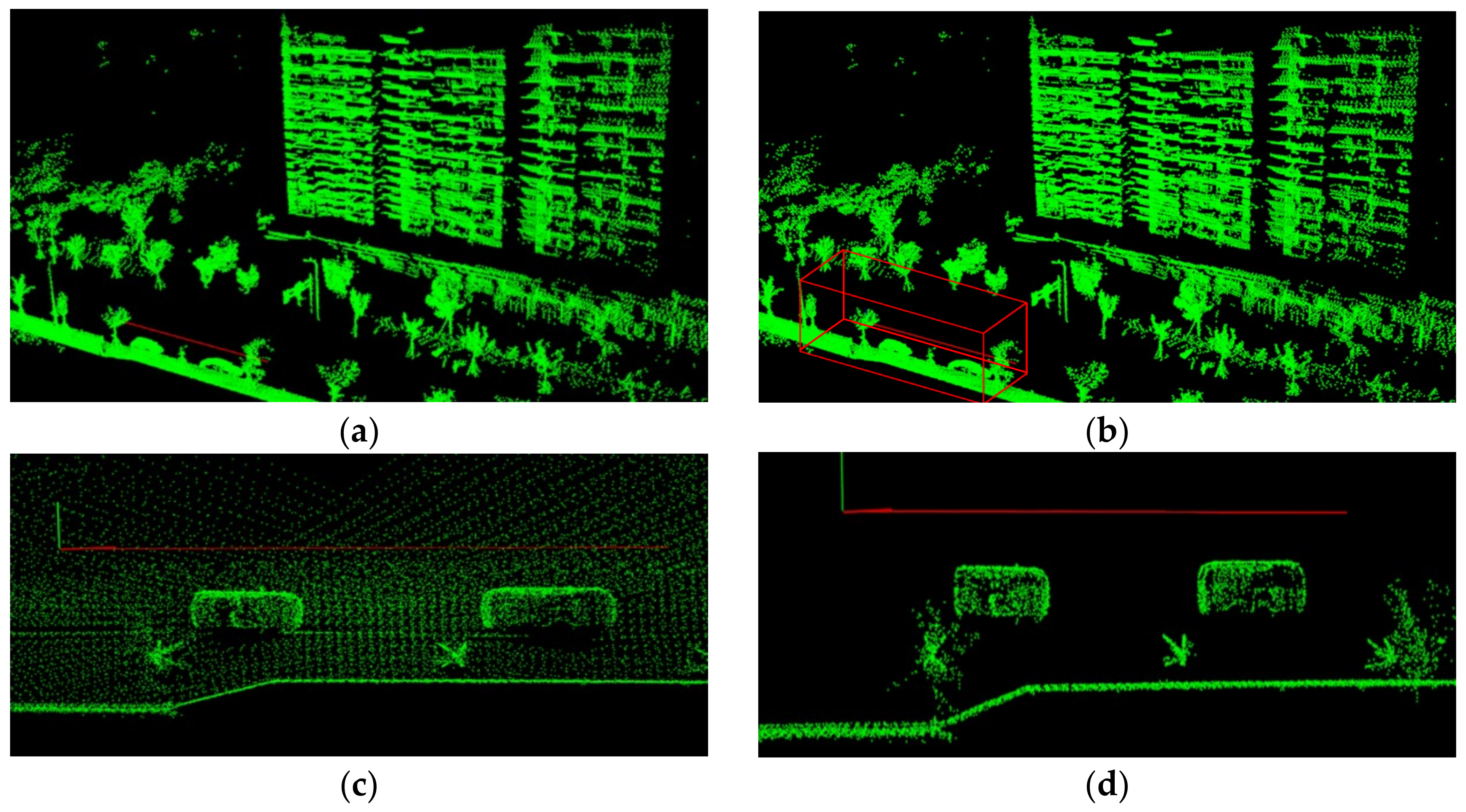
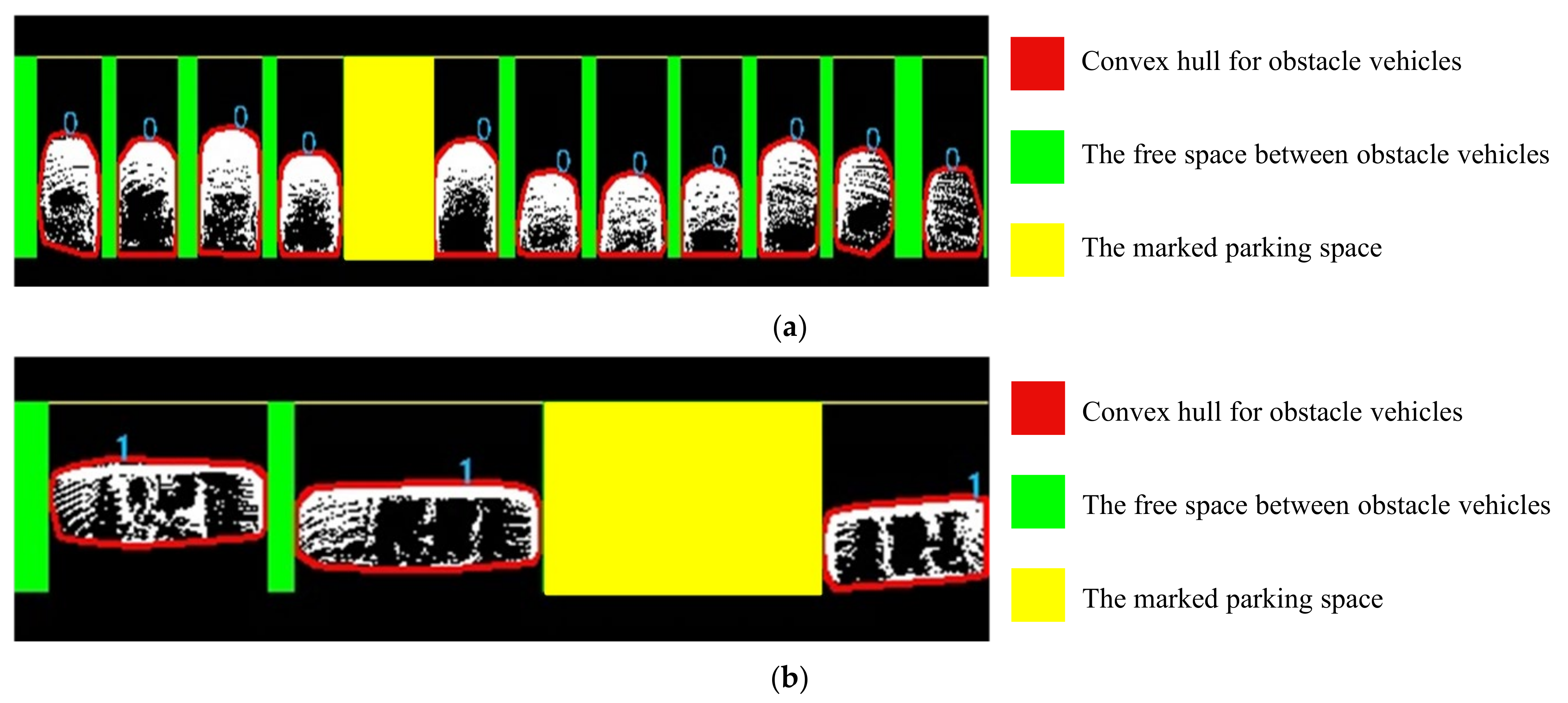
Figure 16 first shows the three-dimensional point cloud map of a test scene and the ground-filtering effect of the ROI. Our method performs well in mapping the scene and filtering ground points within the ROI. The convex hull detection of the obstacle vehicles and the marking of vacant parking spaces are illustrated in Figure 17. The red convex hull line in Figure 17 is a schematic representation of obstacle marking. Figure 17a shows the parking space marking result for perpendicular parking spaces, while Figure 17b depicts the marking result for parallel parking spaces. In Figure 17a, the green area represents the free space between perpendicular obstacle vehicles, and the yellow area indicates the marked perpendicular parking space. In Figure 17b, the green area represents the free space between horizontal obstacle vehicles, and the yellow area indicates the marked horizontal parking space. The number 0 denotes a perpendicular obstacle vehicle, and the number 1 denotes a parallel obstacle vehicle.
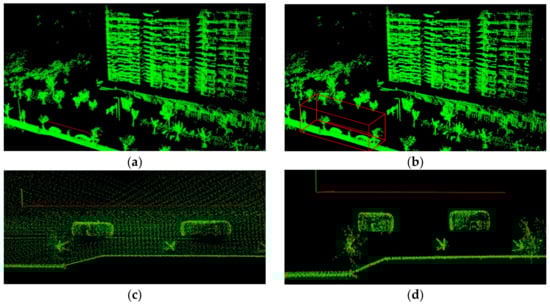
Figure 16.
3D point cloud map of a test scene and ground filtering of the ROI. (a) 3D point cloud map of a test scene; (b) 3D point cloud map of a test scene with an ROI box; (c) Before filtering out ground points in the ROI; (d) After filtering out ground points in the ROI.
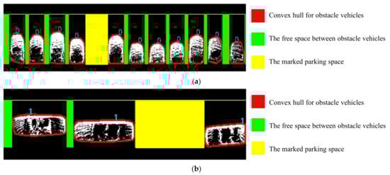
Figure 17.
Schematic diagram of the annotation for obstacle vehicles and parking spaces. (a) Perpendicular obstacle vehicles and perpendicular parking spaces; (b) Parallel obstacle vehicles and parallel parking spaces. “0” recognized the classification label of perpendicular parking mode; And “1” represented horizontal parking mode.
The performance is evaluated using the following parameters and equations:
Table 5 shows the performance evaluation results of the proposed parking space annotation method based on Lidar and IMU. In Table 5, GT, TP, and FP represent the number of existing parking spaces, the number of correctly detected parking spaces, and the number of incorrectly detected parking spaces, respectively. As shown in Table 5, the mean precision and recall of the proposed method are 98.89% and 98.79%, respectively. Compared to the 95.2% precision and 93.6% recall reported in the literature [19], the performance is greatly improved.
Table 5.
Parking space detection performance of the proposed method.
4.2.2. Comparative Experiment
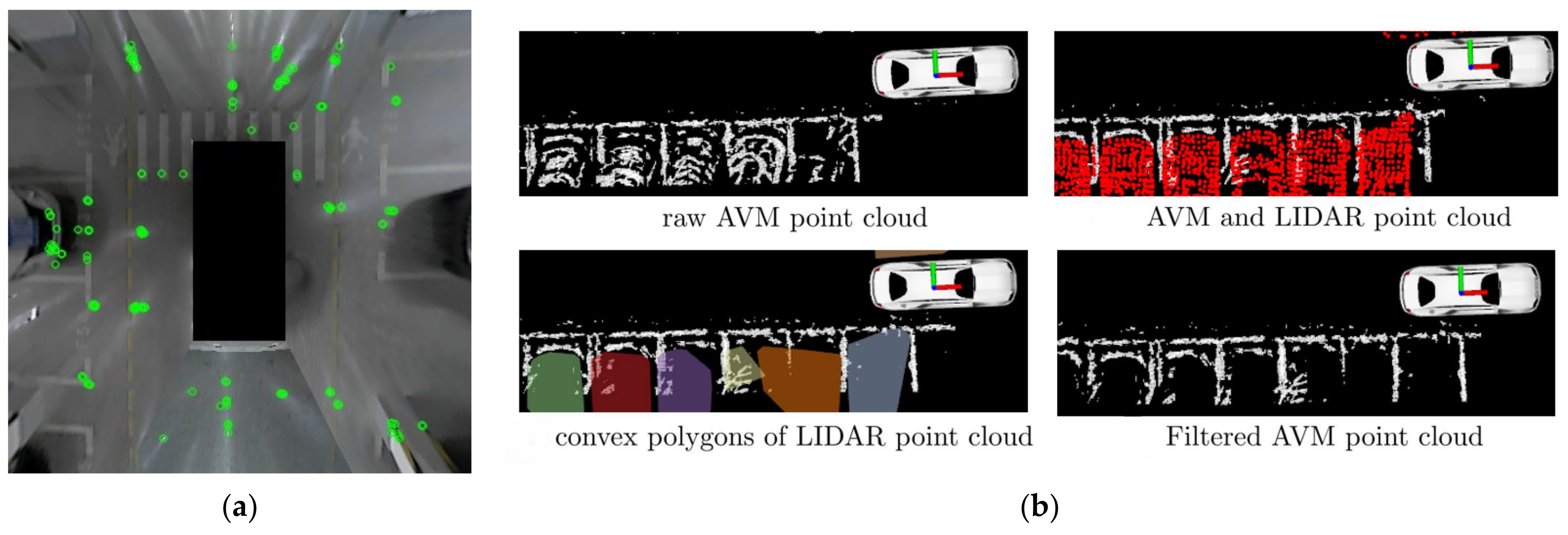
The comparative experiment is based on the open dataset nuScenes. This paper uses the methods proposed in references [3,19] as comparative algorithms. Reference [19] is a Lidar-only method that extracts free space by detecting the 3D information of the vehicle. First, 3D vehicle detection is performed based on the CenterPoint [43]. Then, the parking slots are calculated using the vehicle size and the relative position between the vehicles, and the parking slots are tracked [44]. Finally, a filter method is used to further detect obstacles within the parking space box in the ROI to achieve the final free space detection. Reference [3] is a method that uses visual images as prior map information and combines Lidar recognition to detect empty parking spaces. First, the surround image data of the parking lot is binarized to extract parking line information, which is used as the prior information of the parking space. Secondly, the vehicle point cloud is extracted using Lidar detection data, and then the parking line prior information is superimposed and fused with the vehicle point cloud. Finally, the empty parking space detection result based on visual prior information is obtained.
The algorithm in this paper and the comparative algorithms were tested with open datasets. The schematic diagram of the experimental results is shown in Figure 18, and the experimental results are shown in Table 6.
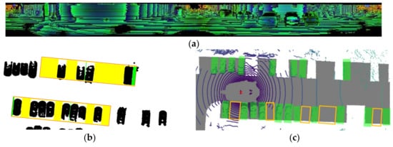

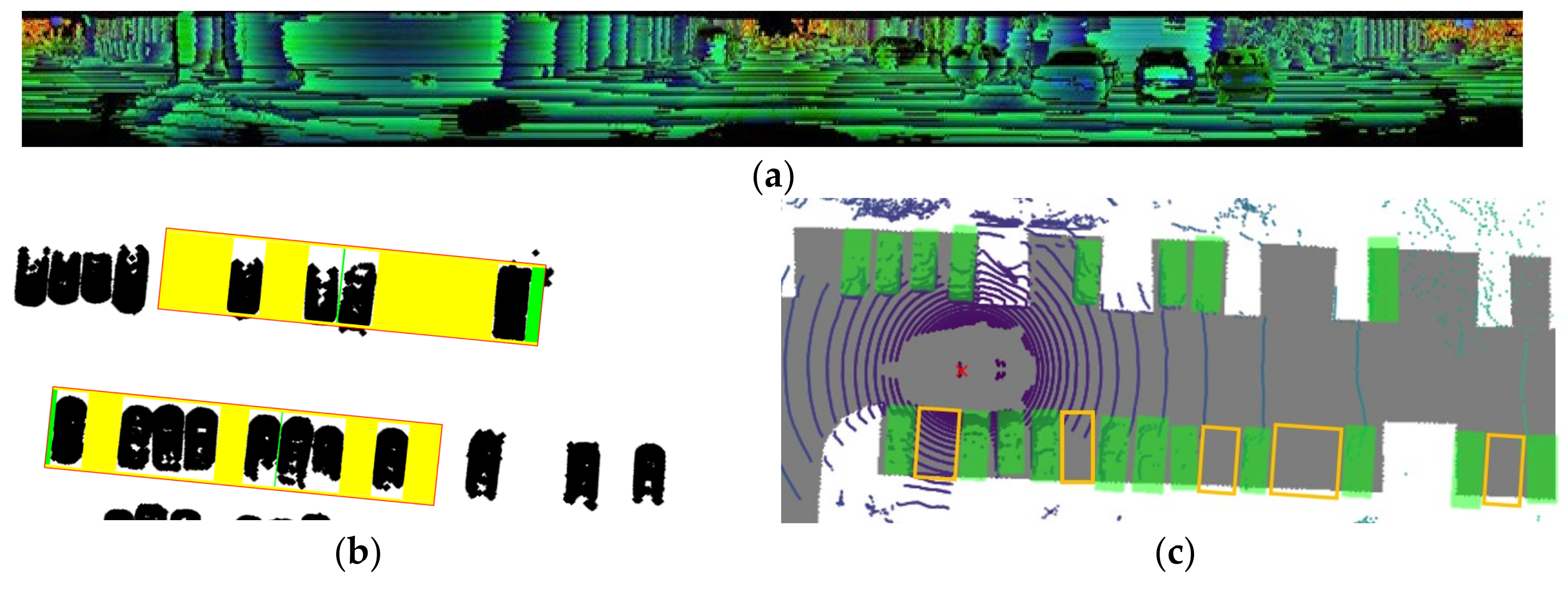
Figure 18.
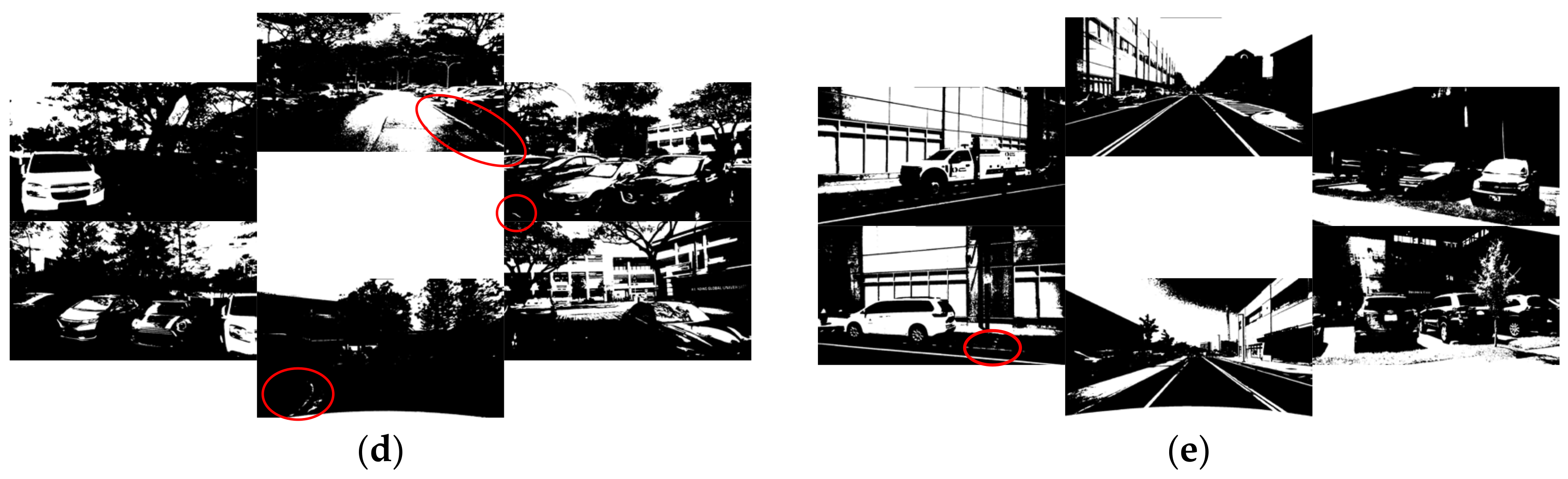
Visualization diagram of free space detection. (a) Polarized matrix visualization of the proposed algorithm in the scene from Figure 15a. Different colors represent different depth values. (b) Free space detection visualization of the proposed algorithm in the scene from Figure 15a: The red rectangle denotes the ROI, the yellow indicates free space meeting the size constraints of the ego vehicle, and the green represents the non-compliant workshop area. (c) Free space detection visualization of the method in reference [19] in the scene from Figure 15a: The green rectangle denotes obstacle vehicles, and the yellow represents free space. (d) Lane line binarization schematic of the method in reference [3] under weak texture conditions, corresponding to Figure 15a: The red circle denotes lane line texture information. The red circle highlights subtle lane line texture under weak lighting conditions, which may be difficult to discern due to minimal pixel intensity differences. (e) Lane line binarization schematic of the method in reference [3] under clear texture but subtle pixel differences due to overexposure, corresponding to Figure 15b.
Table 6.
Comparative parking space detection performance based on the nuScenes datasets.
As depicted in Figure 16, combined with the results presented in Table 6, our method demonstrates superior performance. From a principle analysis perspective, the approach of reference [19] relies on a pre-trained 3D detection and tracking network. The accuracy of this method is influenced by the parameters of the pre-trained network, resulting in a relative number of missed detections of obstacle vehicles. In contrast, our method begins with ground filtering, isolates the ROI and grid map markers, and reduces the impact of noise points on obstacle vehicle recognition. Figure 18d demonstrates the binarization effect of parking lines without corner points in the scene of Figure 15a. The binarization effect shown in Figure 18e corresponds to Figure 15b, where parking lines are marked, but the texture of the ground area and parking lines in the image is similar due to excessive light. While rich visual texture can provide accurate and clear prior map information for parking space recognition, it is heavily influenced by lighting conditions. When texture information is weak or absent, AVM/Lidar fusion [3] fails to deliver satisfactory parking space detection performance, as indicated in Table 6. Whether in parking lots or roadside parking lots, the number of missed parking spaces by this method exceeds 50%. Therefore, compared to both the three-dimensional detection method and the visual prior information-based detection method, the proposed algorithm demonstrates robustness and reliable performance.
We also conducted a supplementary test to verify the significant level of our proposed model across different datasets. We performed a t-test on the local and public datasets nuScenes. The null hypothesis (H0) posits that there is no significant difference in recognition accuracy between the two datasets, implying any observed difference is due to random errors. The alternative hypothesis (H1) suggests that a significant difference exists, indicating the difference is not random. We set the significance level α at 0.05. The results from the local dataset served as the experimental group, while those from the public dataset were the control group. On the local dataset, the average accuracy of parking space recognition was 98.89%, compared to 97.08% on the public dataset. The standard deviations for both groups were calculated as 0.5086 and 0.1470, respectively. Using a one-tailed two-sample t-test with unequal variances, we obtained a t-value significant level of 0.0007, which is much lower than 0.05. Therefore, we accept the null hypothesis and believe that there is no significant difference in the recognition accuracy of the model on the two datasets. This shows that the performance of the model proposed in this paper on different datasets is random, and the performance of the model on the test set is the same as that on the training set or validation set, indicating that the model performs well on unseen data and the performance of the model on these two datasets is stable. In one words, this suggests that the model’s performance is stable across different datasets, demonstrating its robustness on unseen data.
Additionally, we conducted a comparison of storage usage and runtime among different algorithms. We utilized Lidar keyframe point cloud data from scene-0655 in the nuScenes, specifically the parking lot scenario, along with corresponding six-way surround-view image keyframe data. Each point cloud file records the (x, y, z) coordinates, intensity information, and ring index of individual points. This scene comprises 41 keyframes of point cloud and 246 six-way surround-view image keyframes. We evaluated the output storage and runtime storage requirements and runtime of the three algorithms, as summarized in Table 7. While our algorithm shows comparable memory usage during program-execution evaluations, the storage requirements for the polarized matrix and BEV after dimensionality reduction in our method’s output data are significantly lower than those of the original point cloud data. Specifically, although our approach does not have an advantage in time reliability, it achieves a storage space savings of at least 48.38% compared to the comparison algorithm.
Table 7.
Comparison of storage usage between the comparison algorithm and the proposed algorithm.
5. Discussion
In the local dataset verification experiment of the proposed algorithm, Table 5 shows instances of incorrect annotations in some parking space detection results. Through data analysis, two main reasons for these discrepancies have been identified. Firstly, mis-annotations of parking spaces can occur due to discrepancies between actual parking space sizes and preset parameters. For instance, when there are two parking spaces, but the planned parking space size is larger, exceeding the preset parameters, the system may erroneously recognize it as three parking spaces. Secondly, irregular parking behaviors by vehicle owners can also contribute to mis-annotations. For example, in a perpendicular parking slots scenario, two cars parked relatively far apart might leave a space in the middle that meets the preset parking space size, leading the system to detect it as another potential parking spot, resulting in an incorrect count of three parking spaces. Similarly, in a parallel garage setup, two mini cars parked at the ends of adjacent spaces with a space in-between might be interpreted by the system as another available parking space. Thus, the standardization of vehicle parking by drivers has a significant impact on the accuracy of this detection method. However, errors resulting from these issues typically fall within the acceptable margin of error for vehicle constraints.
In the comparative experiment, it was observed that low-lying obstacles have a significant impact on both the proposed algorithm and the method described in the literature [19]. As illustrated in Figure 19, a scene with curbstones in a parking lot from the nuScenes dataset highlights this issue. Referencing Figure 18a, the proposed algorithm detects vehicles using point clouds and utilizes gaps between vehicles to identify free spaces. However, without distinguishing curbstone point clouds, all gaps meeting vehicle size criteria are erroneously identified as free spaces, leading to increased false detections. In contrast, Figure 18b depicts the method from the literature [19], which screens out obstacles within parking slots after determining them, removing detection boxes containing obstacle point clouds. This approach, while reducing false detections, also increases missed detections of obstacles, thereby compromising the robustness of downstream parking functions. Nevertheless, as indicated in Table 6, our algorithm’s F1 score remains largely unaffected. For further algorithm optimization, we propose to explore incorporating an elevation-detection step based on Lidar’s three-dimensional data in our approach in the future. Alternatively, introducing a three-dimensional probability grid map could evaluate obstacle pitch angles using vehicle chassis height as a constraint.
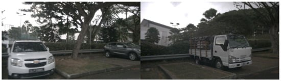
Figure 19.
Some parking spaces in the nuScenes [15] dataset have curbstones next to them.
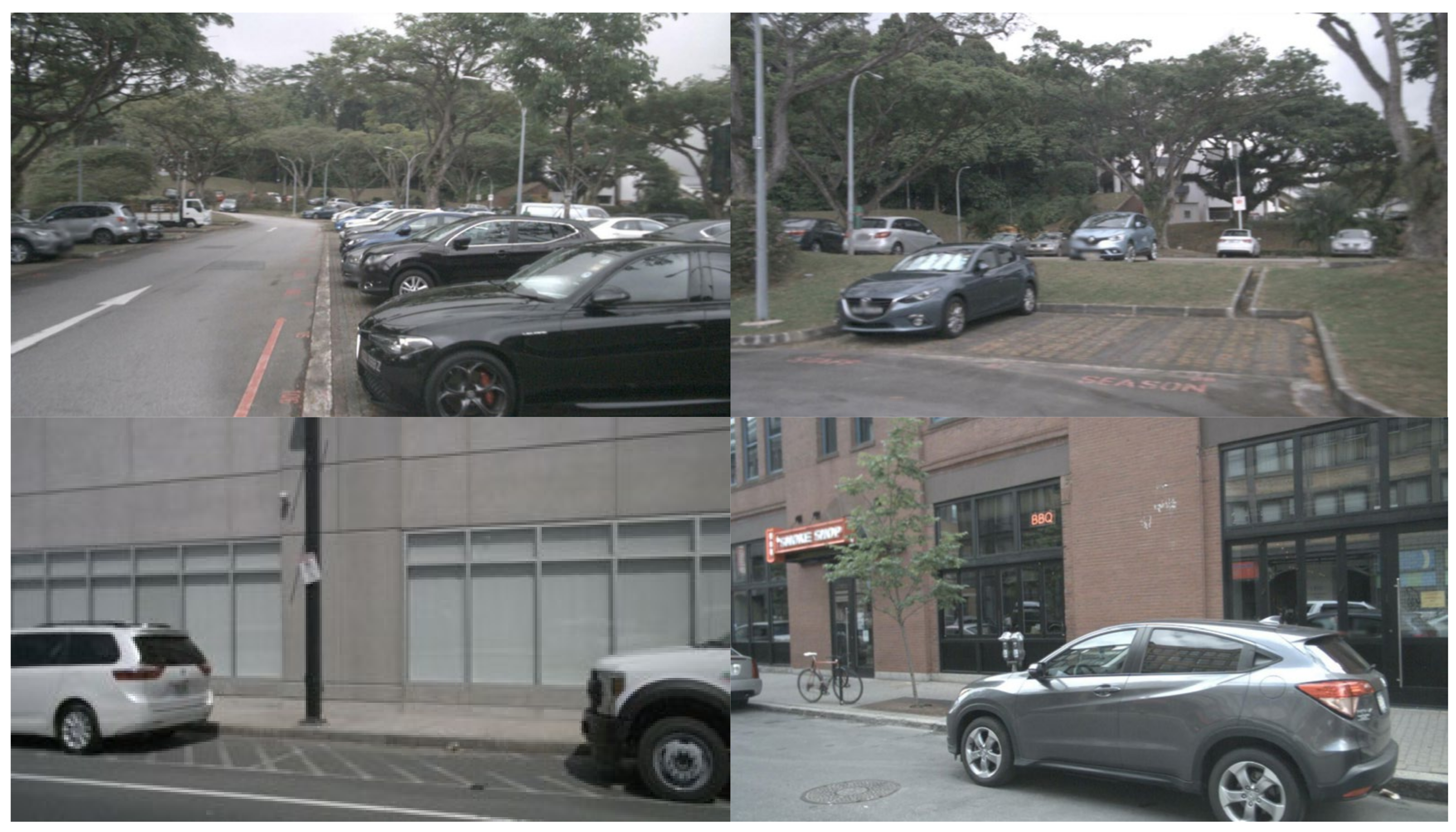
The comparative test results reveal that the parking space detection method relying on visual prior information exhibits poor generalization. Within the nuScenes dataset, certain parking lot scenes lack corner points on parking lines. The non-motorized lane lines of roadside parking are relatively clear, but parking space lines are often blurred, and some real-world scenes may entirely lack parking lines, as depicted in Figure 20. Moreover, visual images are significantly impacted by lighting conditions, resulting in unclear textures in binary images and unreliable detection of parking line corners. Consequently, reliance on visual parking line prior information, as seen in reference [3], leads to substantial gaps in algorithm reliability. In the original text [3], parking space recognition in PL3, which lacks parking lines, is conducted in conjunction with PL1, where parking lines are clear. This dependence implies that recognition in PL3 relies on data from other scenes with visible parking lines. Thus, the visual prior information method proposed in reference [3] is primarily suitable only for scenes featuring distinct parking line textures. An alternative approach to addressing the limited generalization of visual parking space recognition involves pre-building high-precision maps and manually marking parking spaces. However, this method incurs high investment costs and contradicts the goal of cost reduction and efficiency enhancement.
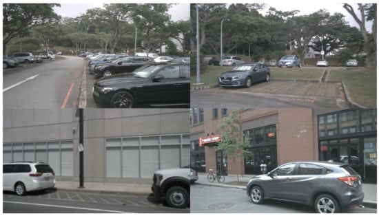
Figure 20.
Some parking spaces in the nuScenes [15] dataset do not have line corners, or the parking space lines are unclear.
In terms of storage usage, the evaluation of the method in literature [19] benefits from reduced model training steps due to loading pre-trained parameters for its 3D object detection process, giving it a certain advantage in parking slot prediction memory usage. However, considering the storage occupancy assessment based on output data, our algorithm demonstrates greater advantages. Specifically, compared to the comparison algorithm [3], our algorithm saves at least 48.38% of storage space, significantly reducing storage costs.
In summary, our algorithm exhibits good performance in terms of effectiveness, accuracy, and robustness in annotating vacant parking spaces.
6. Conclusions
In this paper, we propose a parking space automatic annotation method that tightly couples Lidar with IMU. This method is mainly divided into three parts: tightly coupled pose compensation, point cloud-based scene map construction, and automatic parking space annotation. Tightly coupled pose compensation integrates the pre-integrated IMU with the Lidar frames to perform motion compensation on the fan-shaped sector pose of the Lidar frames, thereby obtaining a more accurate initial pose of the Lidar frames. The point cloud scene map construction utilizes polarized Lidar odometry and loop closure as factors to perform factor graph optimization, resulting in high-precision localization of the vehicle and local map construction. For automatic parking space annotation, we use vehicle dimensions as constraints to fit straight lines for obstacle vehicles on the local map after BEV projection. The free space between the fitted straight lines is then identified as parking spaces for annotation. Our method employs dual dimensionality reductions through polarized and BEV, enabling it to overcome issues such as heavy three-dimensional data processing, insufficient lighting, and unclear textures in image, signal occlusion, and odometry accumulation errors. It directly performs parking space annotation for vehicles in unknown environments, achieving better accuracy and recall rates compared to comparative algorithms. Specifically, it achieves a precision of 98.89% and a recall of 98.79% on our local dataset and a precision of 97.08% and a recall of 99.40% on the nuScenes dataset, while also reducing storage by 48.38% in the open dataset. It is important to note that, due to the absence of angled parking spots in the nuScenes dataset, the effectiveness of automatic annotation for oblique parking spaces has only been evaluated using the local dataset. In the next phase of our research, we plan to collect a wider variety of parking lots data for further analysis and will also explore the possibility of creating a publicly accessible dataset.
Certainly, our algorithm inevitably faces challenges. Specifically, when encountering low-lying obstacles, it may misjudge, compromising accuracy and potentially posing a risk to the vehicle. To enhance generalization capabilities, we aim to explore incorporating a pitch angle obstacle-detection approach, leveraging Lidar’s three-dimensional data while adhering to the constraints imposed by the vehicle’s chassis height. Furthermore, it is noteworthy that the Lidar and IMU devices instrumental to our system, while prevalent in scientific research, have yet to gain widespread commercial adoption due to their substantial costs. In future research, we aim to expand our studies to include a comparative analysis of various IMU and Lidar sensors with differing specifications. This will allow us to investigate how variations in sensor parameters affect the accuracy and robustness of our parking space annotation method. Nevertheless, addressing hardware costs and commercialization falls outside the immediate purview of our development. We envision exploring this domain in future endeavors, contemplating strategies such as leveraging cost-effective Lidar solutions and low-cost localization equipment to develop high-precision parking space annotation techniques, thereby addressing this challenge.
Author Contributions
Conceptualization, J.C. and F.L.; Methodology, J.C., F.L. and X.L.; Software, J.C., F.L. and Y.Y.; Validation, J.C. and Y.Y.; Formal analysis, J.C. and F.L.; Investigation, J.C. and F.L.; Writing—original draft preparation, J.C.; Writing—review and editing, J.C. and X.L.; Visualization, J.C.; Supervision, X.L.; Project administration, X.L.; Funding acquisition, X.L. All authors have read and agreed to the published version of the manuscript.
Funding
This research was funded by the National Natural Science Foundation of China, grant number U20A20193.
Institutional Review Board Statement
Not applicable.
Informed Consent Statement
Not applicable.
Data Availability Statement
The data presented in this study are available on request from the corresponding author. The data are not publicly available due to privacy or ethical restrictions.
Conflicts of Interest
The authors declare no conflicts of interest.
References
- Yamada, S.; Watanabe, Y.; Kanamori, R.; Sato, K.; Takada, H. Estimation Method of Parking Space Conditions Using Multiple 3D-LiDARs. Int. J. Intell. Transp. Syst. Res. 2022, 20, 422–432. [Google Scholar] [CrossRef]
- Li, F.; Chen, J.; Yuan, Y.; Hu, Z.; Liu, X. Enhanced Berth Mapping and Clothoid Trajectory Prediction Aided Intelligent Underground Localization. Appl. Sci. 2024, 14, 5032. [Google Scholar] [CrossRef]
- Im, G.; Kim, M.; Park, J. Parking Line Based SLAM Approach Using AVM/LiDAR Sensor Fusion for Rapid and Accurate Loop Closing and Parking Space Detection. Sensors 2019, 19, 4811. [Google Scholar] [CrossRef] [PubMed]
- Hasan Yusuf, F.; Mangoud, M.A. Real-Time Car Parking Detection with Deep Learning in Different Lighting Scenarios. Int. J. Comput. Digit. Syst. 2024, 15, 1–9. [Google Scholar] [CrossRef]
- Gkolias, K.; Vlahogianni, E.I. Convolutional Neural Networks for On-Street Parking Space Detection in Urban Networks. IEEE Trans. Intell. Transp. Syst. 2019, 20, 4318–4327. [Google Scholar] [CrossRef]
- Jiang, S.; Jiang, H.; Ma, S.; Jiang, Z. Detection of Parking Slots Based on Mask R-CNN. Appl. Sci. 2020, 10, 4295. [Google Scholar] [CrossRef]
- Ma, Y.; Liu, Y.; Zhang, L.; Cao, Y.; Guo, S.; Li, H. Research Review on Parking Space Detection Method. Symmetry 2021, 13, 128. [Google Scholar] [CrossRef]
- Zainal Abidin, M.; Pulungan, R. A Systematic Review of Machine-Vision-Based Smart Parking Systems. Sci. J. Inform. 2020, 7, 213–227. [Google Scholar] [CrossRef]
- Hwang, J.-H.; Cho, B.; Choi, D.-H. Feature Map Analysis of Neural Networks for the Application of Vacant Parking Slot Detection. Appl. Sci. 2023, 13, 10342. [Google Scholar] [CrossRef]
- Kumar, K.; Singh, V.; Raja, L.; Bhagirath, S.N. A Review of Parking Slot Types and Their Detection Techniques for Smart Cities. Smart Cities 2023, 6, 2639–2660. [Google Scholar] [CrossRef]
- Thakur, N.; Bhattacharjee, E.; Jain, R.; Acharya, B.; Hu, Y.-C. Deep Learning-Based Parking Occupancy Detection Framework Using ResNet and VGG-16. Multimed. Tools Appl. 2024, 83, 1941–1964. [Google Scholar] [CrossRef]
- Luo, Q.; Saigal, R.; Hampshire, R.; Wu, X. A Statistical Method for Parking Spaces Occupancy Detection via Automotive Radars 2016. In Proceedings of the 2017 IEEE 85th Vehicular Technology Conference (VTC Spring), Sydney, NSW, Australia, 4–7 June 2017. [Google Scholar]
- Jiang, H.; Chen, Y.; Shen, Q.; Yin, C.; Cai, J. Semantic Closed-Loop Based Visual Mapping Algorithm for Automated Valet Parking. Proc. Inst. Mech. Eng. Part J. Automob. Eng. 2023, 238, 2091–2104. [Google Scholar] [CrossRef]
- Ye, D.; Yin, X.; Dong, M. Research on Vehicle Parking Aid System Based on Parking Image Enhancement. In Proceedings of the Communications, Signal Processing, and Systems, Online, 18–20 March 2022; Liang, Q., Wang, W., Liu, X., Na, Z., Zhang, B., Eds.; Springer: Singapore, 2022; pp. 192–200. [Google Scholar]
- Fong, W.K.; Mohan, R.; Hurtado, J.V.; Zhou, L.; Caesar, H.; Beijbom, O.; Valada, A. Panoptic nuScenes: A Large-Scale Benchmark for LiDAR Panoptic Segmentation and Tracking. IEEE Robot. Autom. Lett. 2021, 7, 3795–3802. [Google Scholar] [CrossRef]
- Kamiyama, T.; Maeyama, S.; Okawa, K.; Watanabe, K.; Nogami, Y. Recognition of Parking Spaces on Dry and Wet Road Surfaces Using Received Light Intensity of Laser for Ultra Small EVs. In Proceedings of the 2019 IEEE/SICE International Symposium on System Integration (SII), Paris, France, 14–16 January 2019; pp. 494–501. [Google Scholar]
- Gong, Z.; Li, J.; Luo, Z.; Wen, C.; Wang, C.; Zelek, J. Mapping and Semantic Modeling of Underground Parking Lots Using a Backpack LiDAR System. IEEE Trans. Intell. Transp. Syst. 2021, 22, 734–746. [Google Scholar] [CrossRef]
- Jiménez, F.; Clavijo, M.; Cerrato, A. Perception, Positioning and Decision-Making Algorithms Adaptation for an Autonomous Valet Parking System Based on Infrastructure Reference Points Using One Single LiDAR. Sensors 2022, 22, 979. [Google Scholar] [CrossRef] [PubMed]
- Yang, W.; Li, D.; Xu, W.; Zhang, Z. A LiDAR-Based Parking Slots Detection System. Int. J. Automot. Technol. 2024, 25, 331–338. [Google Scholar] [CrossRef]
- Li, L.; Shum, H.P.H.; Breckon, T.P. Less Is More: Reducing Task and Model Complexity for 3D Point Cloud Semantic Segmentation. In Proceedings of the 2023 IEEE/CVF Conference on Computer Vision and Pattern Recognition (CVPR), Vancouver, BC, Canada, 17–24 June 2023; pp. 9361–9371. [Google Scholar]
- Tong, L.; Cheng, L.; Li, M.; Wang, J.; Du, P. Integration of LiDAR Data and Orthophoto for Automatic Extraction of Parking Lot Structure. IEEE J. Sel. Top. Appl. Earth Obs. Remote Sens. 2014, 7, 503–514. [Google Scholar] [CrossRef]
- Zhang, J.; Singh, S. LOAM: Lidar Odometry and Mapping in Real-Time. In Proceedings of the Robotics: Science and Systems X, Robotics: Science and Systems Foundation, Berkeley, CA, USA, 12–16 July 2014. [Google Scholar]
- Rozenberszki, D.; Majdik, A. LOL: Lidar-Only Odometry and Localization in 3D Point Cloud Maps. In Proceedings of the 2020 IEEE International Conference on Robotics and Automation (ICRA), online, 31 May–31 August 2020. [Google Scholar]
- Balazadegan Sarvrood, Y.; Hosseinyalamdary, S.; Gao, Y. Visual-LiDAR Odometry Aided by Reduced IMU. ISPRS Int. J. Geo-Inf. 2016, 5, 3. [Google Scholar] [CrossRef]
- Koide, K.; Yokozuka, M.; Oishi, S.; Banno, A. Globally Consistent and Tightly Coupled 3D LiDAR Inertial Mapping. In Proceedings of the 2022 International Conference on Robotics and Automation (ICRA), Philadelphia, PA, USA, 23–27 May 2022; pp. 5622–5628. [Google Scholar] [CrossRef]
- Liu, Z.; Li, Z.; Liu, A.; Shao, K.; Guo, Q.; Wang, C. LVI-Fusion: A Robust Lidar-Visual-Inertial SLAM Scheme. Remote Sens. 2024, 16, 1524. [Google Scholar] [CrossRef]
- Shan, T.; Englot, B.; Meyers, D.; Wang, W.; Ratti, C.; Rus, D. LIO-SAM: Tightly-Coupled Lidar Inertial Odometry via Smoothing and Mapping. In Proceedings of the 2020 IEEE/RSJ International Conference on Intelligent Robots and Systems (IROS), Las Vegas, NV, USA, 25–29 October 2020; pp. 5135–5142. [Google Scholar]
- Zuo, X.; Geneva, P.; Lee, W.; Liu, Y.; Huang, G. LIC-Fusion: LiDAR-Inertial-Camera Odometry. In Proceedings of the 2019 IEEE/RSJ International Conference on Intelligent Robots and Systems (IROS), Macau, China, 3–8 November 2019; pp. 5848–5854. [Google Scholar] [CrossRef]
- Zhao, S.; Zhang, H.; Wang, P.; Nogueira, L.; Scherer, S. Super Odometry: IMU-Centric LiDAR-Visual-Inertial Estimator for Challenging Environments. In Proceedings of the 2021 IEEE/RSJ International Conference on Intelligent Robots and Systems (IROS), Prague, Czech Republic, 27 September–1 October 2021; pp. 8729–8736. [Google Scholar] [CrossRef]
- Shan, T.; Englot, B.; Ratti, C.; Rus, D. LVI-SAM: Tightly-Coupled Lidar-Visual-Inertial Odometry via Smoothing and Mapping. In Proceedings of the 2021 IEEE International Conference on Robotics and Automation (ICRA), Xi’an, China, 30 May–5 June 2021. [Google Scholar]
- Xu, W.; Zhang, F. FAST-LIO: A Fast, Robust LiDAR-Inertial Odometry Package by Tightly-Coupled Iterated Kalman Filter. IEEE Robot. Autom. Lett. 2021, 6, 3317–3324. [Google Scholar] [CrossRef]
- Zhang, Y. LILO: A Novel Lidar–IMU SLAM System With Loop Optimization. IEEE Trans. Aerosp. Electron. Syst. 2022, 58, 2649–2659. [Google Scholar] [CrossRef]
- Rusinkiewicz, S.; Levoy, M. Efficient Variants of the ICP Algorithm. In Proceedings of the Proceedings Third International Conference on 3-D Digital Imaging and Modeling, Quebec City, QC, Canada, 28 May–1 June 2001; pp. 145–152. [Google Scholar]
- Segal, A.; Haehnel, D.; Thrun, S. Generalized-ICP. In Proceedings of the Robotics: Science and Systems V—Robotics: Science and Systems Foundation, Seattle, WA, USA, 28 June–1 July 2009. [Google Scholar]
- Biber, P.; Strasser, W. The Normal Distributions Transform: A New Approach to Laser Scan Matching. In Proceedings of the Proceedings 2003 IEEE/RSJ International Conference on Intelligent Robots and Systems (IROS 2003) (Cat. No.03CH37453), Las Vegas, NV, USA, 27–31 October 2003; Volume 3, pp. 2743–2748. [Google Scholar]
- Aoki, Y.; Goforth, H.; Srivatsan, R.A.; Lucey, S. PointNetLK: Robust & Efficient Point Cloud Registration Using PointNet. In Proceedings of the IEEE/CVF Conference on Computer Vision and Pattern Recognition (CVPR), Long Beach, CA, USA, 15–20 June 2019. [Google Scholar]
- Yuan, W.; Eckart, B.; Kim, K.; Jampani, V.; Fox, D.; Kautz, J. DeepGMR: Learning Latent Gaussian Mixture Models for Registration. In Proceedings of the Computer Vision–ECCV 2020: 16th European Conference, Glasgow, UK, 23–28 August 2020; Springer International Publishing: Cham, Switzerland, 2020. [Google Scholar]
- Forster, C.; Carlone, L.; Dellaert, F.; Scaramuzza, D. On-Manifold Preintegration for Real-Time Visual–Inertial Odometry. IEEE Trans. Robot. 2017, 33, 1–21. [Google Scholar] [CrossRef]
- Kaess, M.; Johannsson, H.; Roberts, R.; Ila, V.; Leonard, J.J.; Dellaert, F. iSAM2: Incremental Smoothing and Mapping Using the Bayes Tree. Int. J. Robot. Res. 2012, 31, 216–235. [Google Scholar] [CrossRef]
- Zhang, J.; Singh, S. Low-Drift and Real-Time Lidar Odometry and Mapping. Auton. Robots 2017, 41, 401–416. [Google Scholar] [CrossRef]
- Shan, T.; Englot, B. LeGO-LOAM: Lightweight and Ground-Optimized Lidar Odometry and Mapping on Variable Terrain. In Proceedings of the 2018 IEEE/RSJ International Conference on Intelligent Robots and Systems (IROS), Madrid, Spain, 1–5 October 2018; pp. 4758–4765. [Google Scholar]
- Himmelsbach, M.; Hundelshausen, F.V.; Wuensche, H.-J. Fast Segmentation of 3D Point Clouds for Ground Vehicles. In Proceedings of the 2010 IEEE Intelligent Vehicles Symposium, La Jolla, CA, USA, 21–24 June 2010; pp. 560–565. [Google Scholar]
- Yin, T.; Zhou, X.; Krahenbuhl, P. Center-Based 3D Object Detection and Tracking. In Proceedings of the 2021 IEEE/CVF Conference on Computer Vision and Pattern Recognition (CVPR), Nashville, TN, USA, 20–25 June 2021; pp. 11779–11788. [Google Scholar] [CrossRef]
- Zhou, J.; Navarro-Serment, L.E.; Hebert, M. Detection of Parking Spots Using 2D Range Data. In Proceedings of the 2012 15th International IEEE Conference on Intelligent Transportation Systems, Anchorage, AK, USA, 16–19 September 2012; pp. 1280–1287. [Google Scholar]


Disclaimer/Publisher’s Note: The statements, opinions and data contained in all publications are solely those of the individual author(s) and contributor(s) and not of MDPI and/or the editor(s). MDPI and/or the editor(s) disclaim responsibility for any injury to people or property resulting from any ideas, methods, instructions or products referred to in the content. |
© 2024 by the authors. Licensee MDPI, Basel, Switzerland. This article is an open access article distributed under the terms and conditions of the Creative Commons Attribution (CC BY) license (https://creativecommons.org/licenses/by/4.0/).