High-Precision Elastoplastic Four-Node Quadrilateral Shell Element

Abstract

In order to enhance the accuracy of calculations for four-node quadrilateral shell elements, modifications have to be made to the computation of the membrane strain rate and transverse shear strain rate. For membrane strain rate calculations, the interpolation of the quadratic displacement of the nodes along the edges of the quadrilateral shell element is implemented, along with the introduction of a degree of freedom for rotation around the normal. Additionally, the elimination of the zero-energy mode of additional stiffness is achieved through a penalty function. When computing the transverse shear strain rate, the covariant component is expressed in the tensor of the natural coordinate system, followed by the elimination of shear self-locking in the element coordinate system. The strain-updating calculation and stress-updating calculation for the quadrilateral shell element, utilizing the model and J2 flow theory, respectively, are suitable for small deformations, geometric nonlinearity, and elastic–plastic problems. The improved quadrilateral shell element successfully undergoes in-plane and bending fragment inspections, demonstrating good reliability and calculation accuracy for the dynamic analysis of planar shells, curved shells, and twisted shells.

1. Introduction

In engineering, various shell elements have been developed [1,2,3,4,5,6], including the folded shell element, which is created by combining plane stress and plate bending elements, as well as the degenerate shell element, derived from the shell element hypothesis based on three-dimensional entity theory. The quadrilateral shell element, recognized for its simple structure and versatility, is widely utilized across different industries. However, the development of quadrilateral shell elements with enhanced accuracy presents a significant challenge, particularly in terms of addressing shear and membrane locking effects [7]. These issues can greatly affect the accuracy of solutions for plane stress and transverse shear problems, leading to substantial discrepancies between the calculated and actual results [8,9].

The traditional quadrilateral shell element is limited by its inability to permit rotation around the normal vector of the neutral plane, which complicates the solution of plane stress problems and exacerbates the issue of film self-locking. The phenomenon of membrane self-locking has been extensively investigated in three-node curved beams and nine-node shell elements [10,11,12], leading to the proposal of various methods aimed at mitigating this issue. An improved four-node quadrilateral shell element [13,14,15] has been developed that incorporates a degree of freedom for rotation around the normal vector of the neutral plane. Although the Belytschko and Leviathan [16] units can function within a general six-DOF framework, the innovative projection scheme employed means that the sixth rotational degree of freedom does not represent a true degree of freedom. While certain specialized techniques can be used to address this limitation, the optimal solution remains a unit that allows for rotation around the normal.

The methods developed by Allman [17], Cook [18], Yunus [19], and Huang [20] have been employed to introduce quadratic functions for the interpolation of the element edges. This approach aims to eliminate the translational displacement of the edge midpoint and provide adjacent angular nodes with rotational degrees of freedom around the normal. Consequently, the four-node quadrilateral shell element mitigates the effects of membrane self-locking. However, the introduction of rotational degrees of freedom around the normal results in a redundant zero-energy mode, which does not possess physical significance. MacNeal [21] addresses the zero-energy mode by incorporating additional stiffness through a penalty function, effectively simulating the strain induced by the rotational degrees of freedom around the normal.

Bathe [22,23] proposed four-node and eight-node shell elements (MITC4 and MITC8) utilizing the mixed tensor interpolation strain method [24,25]. When calculating the transverse shear strain rate, the covariant component is expressed through tensor interpolation in the natural coordinate system and subsequently transformed to the element coordinate system, thereby eliminating shear self-locking.

In the context of elastoplastic problems, the stress is updated according to the J2 flow theory [26,27,28,29,30]. The second invariant function of the skew stress tensor is employed to assess whether the yield condition has been met, thereby indicating the transition to the plastic stage. The cumulative equivalent plastic strain is derived by calculating the increment in the equivalent plastic strain using the radial return method, while simultaneously updating the back stress and yield stress. Additionally, the tentative deviatoric stress is proportionally reduced to return to the yield surface. It is important to note that the relationship between the yield stress and plasticity is expected to be linear (i.e., linear strengthening). By introducing a specific parameter, the unified representation of ideal elastic–plastic [31,32], isotropichardening [33,34], kinematic hardening [35,36], and mixed hardening models [37] can be achieved.

In this study, we modify the four-node quadrilateral shell element, which possesses three translational and three rotational DOFs per node, and update the membrane strain rate and bending strain rate. By interpolating the quadratic displacement of the quadrilateral shell element, we introduce a degree of freedom for rotation around the normal direction, thereby mitigating the effects of film self-locking. To address the zero-energy mode associated with the rotational degree of freedom, we incorporate additional stiffness. The covariant components are expressed as tensors in natural coordinates and subsequently transformed into the element coordinate system to eliminate shear self-locking. This research employs a method that modifies both the membrane and transverse shear strain rates to investigate the elastic–plastic behavior of the four-node quadrilateral shell element, with the goal of enhancing the calculation accuracy.

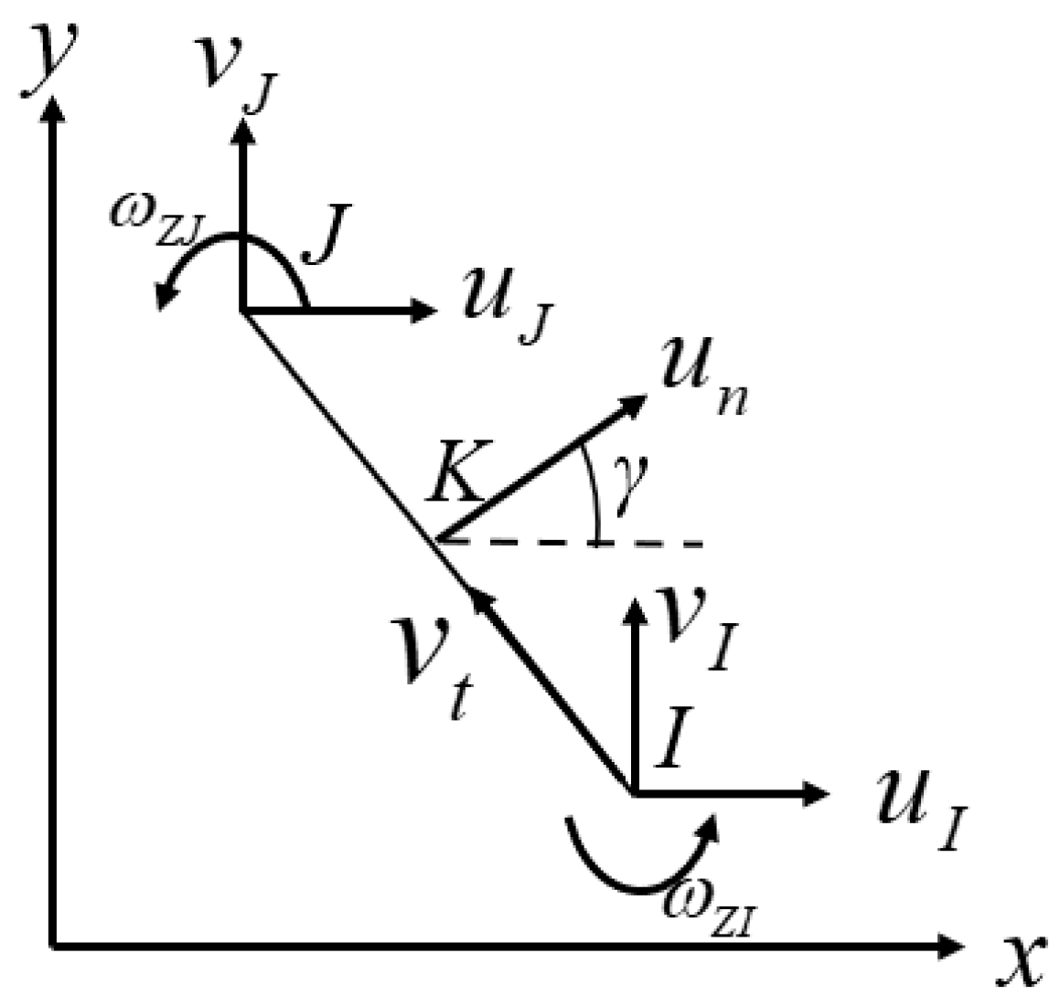
2. Introduction to DOF of Rotation around Element Normal

The method proposed by Allman [17] is employed to interpolate the secondary displacement of the nodes located at the edges of the quadrilateral shell element, incorporating a degree of freedom for rotation about the element’s normal. As illustrated in Figure 1, the displacement of node K on the IJ side can be expressed as follows:

$$\begin{array}{l}{u}_K={\displaystyle \frac{u_I+u_J}{2}}+{\displaystyle \frac{y_J-y_I}{8}}({\omega }_{ZJ}-{\omega }_{ZI})\\ v_K={\displaystyle \frac{v_I+v_J}{2}}-{\displaystyle \frac{x_J-x_I}{8}}({\omega }_{ZJ}-{\omega }_{ZI})\end{array}$$

(1)

In a quadrilateral element with middle nodes, the interpolation function of displacement u and v is

$$u={\tilde{N}}_I{u}_{I}v={\tilde{N}}_I{v}_I$$

(2)

where the uppercase subscripts I, J, and K represent the node number, the repeated uppercase subscripts signify the conventional summation, and ${\tilde{N}}_I$ is the standard eight-node serendipity interpolation basis function.

$$\begin{array}{l}{\tilde{N}}_I=0.25\left(1+\xi {\xi }_I\right)\left(1+\eta {\eta }_I\right)\left(\xi {\xi }_I+\eta {\eta }_I-1\right)\left(\mathrm{I}=1,2,3,4\right)\\ {\tilde{N}}_I=0.5\left(1-{\xi }^2\right)\left(1+\eta {\eta }_I\right)\left(\mathrm{I}=5,7\right)\\ {\tilde{N}}_I=0.5\left(1+\xi {\xi }_I\right)\left(1-{\eta }^2\right)\left(\mathrm{I}=6,8\right)\end{array}$$

(3)

where ${\xi }_I=\left[\begin{array}{cccccccc}-1& 0& 1& 1& 1& 0& -1& -1\end{array}\right]$, ${\eta }_I=\left[\begin{array}{cccccccc}-1& -1& -1& 0& 1& 1& 1& 0\end{array}\right]$.

In quadrilateral elements with intermediate nodes, each edge of the element is consistent with a three-node straight line, and the intermediate nodes on each edge of the element can be expressed according to Equation (1). All middle nodes of a quadrilateral shell element are acquired by introducing them into Equation (2) as per Equation (1).

$$u=N_I{u}_I+N_I^u{\omega }_{ZI}v=N_I{v}_I+N_I^v{\omega }_{ZI}$$

(4)

where $N_I$ is the interpolation basis function of four standard nodes,

$$N_I=0.25\left(1+\xi {\xi }_I\right)\left(1+\eta {\eta }_I\right)\left(\mathrm{I}=1,2,3,4\right)$$

(5)

$N_I^u$ and $N_I^v$ are ${\omega }_I$ corresponding to the interpolation basis function of u and v.

$$\begin{array}{l}{N}_1^u=0.125(y_{14}{\tilde{N}}_8+y_{12}{\tilde{N}}_5)N_2^u=0.125(y_{21}{\tilde{N}}_5+y_{23}{\tilde{N}}_6)\\ N_3^u=0.125(y_{32}{\tilde{N}}_6+y_{34}{\tilde{N}}_7)N_4^u=0.125(y_{43}{\tilde{N}}_7+y_{41}{\tilde{N}}_8)\end{array}$$

(6)

$$\begin{array}{l}{N}_1^v=-0.125(x_{14}{\tilde{N}}_8+x_{12}{\tilde{N}}_5)N_2^v=-0.125(x_{21}{\tilde{N}}_8+x_{23}{\tilde{N}}_5)\\ N_3^v=-0.125(x_{32}{\tilde{N}}_8+x_{34}{\tilde{N}}_5)N_4^v=-0.125(x_{43}{\tilde{N}}_8+x_{41}{\tilde{N}}_5)\end{array}$$

(7)

where $y_{IJ}=y_I-y_J$, $x_{IJ}=x_I-x_J$.

According to the Mindlin–Reissner formula, the complete three-dimensional velocity field of the shell element is

$$V_i(\xi ,\eta ,\zeta )=N_I^{3D}(\xi ,\eta ,\zeta )V_{iI}$$

(8)

where $N_I^{3D}$ denotes the full three-dimensional isoparametric shape functions, $V_i=\left[\begin{array}{ccc}u& v& w\end{array}\right]$. The symbols in Equation (8) and Equation (4) have different meanings. Equation (4) represents the two-dimensional velocity field, while Equation (8) represents the complete three-dimensional velocity field. Since the normals remain straight, we can write

$$V_i(\xi ,\eta ,\zeta )=N_I\left[V_{iI}+{\displaystyle \frac{a}{2}}\zeta (-{\delta }_{i2}{\omega }_{xI}+{\delta }_{i1}{\omega }_{yI})\right]$$

(9)

where a is the thickness, Equation (4) is brought into Equation (9), where u and v are expressed as

$$\begin{array}{l}u=N_I{u}_I+N_I^u{\omega }_{zI}+N_I{\displaystyle \frac{a}{2}}\varsigma {\omega }_{yI}\\ v=N_I{v}_I+N_I^{\mathrm{v}}{\omega }_{\mathrm{z}I}-N_I{\displaystyle \frac{a}{2}}\varsigma {\omega }_{xI}\end{array}$$

(10)

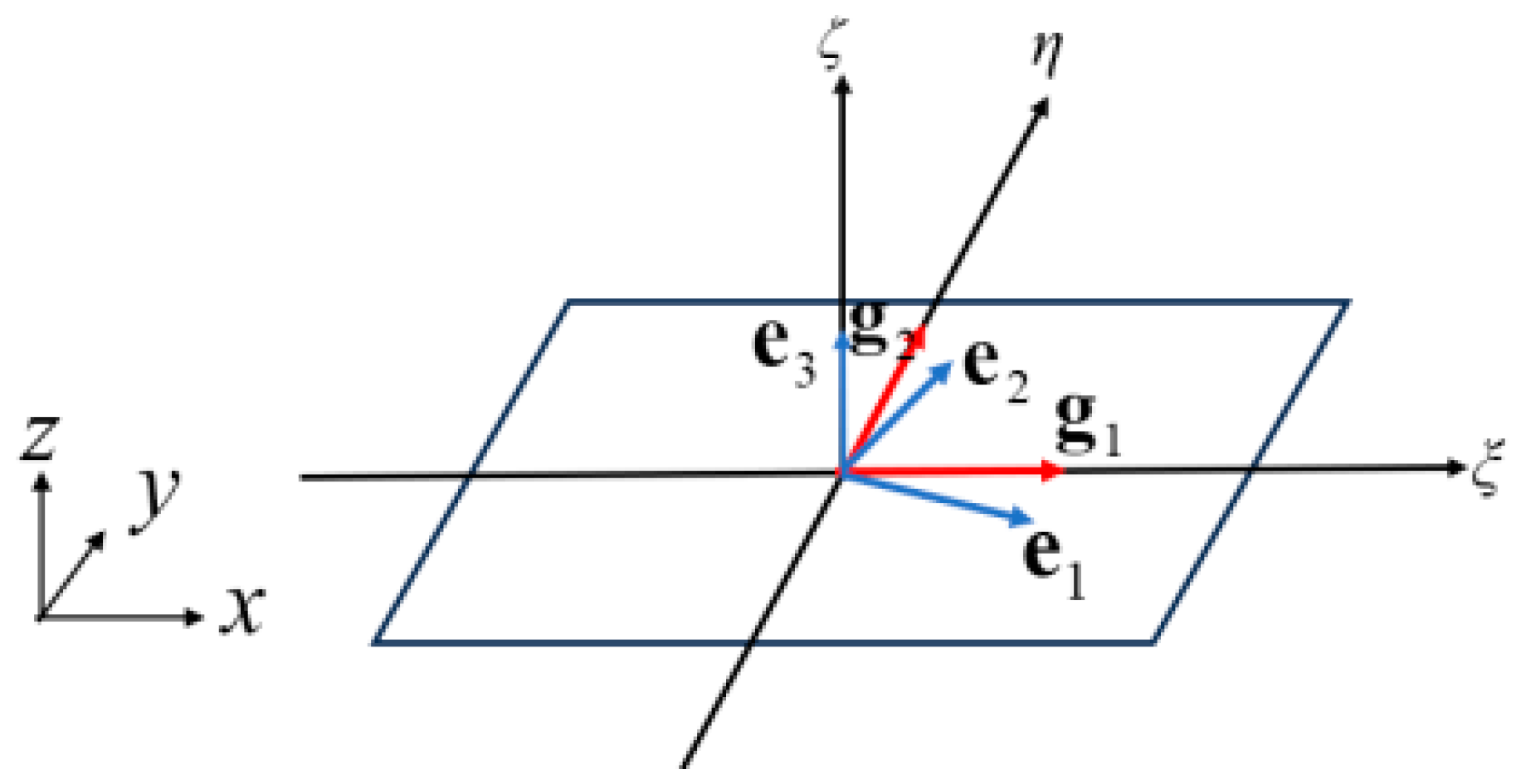
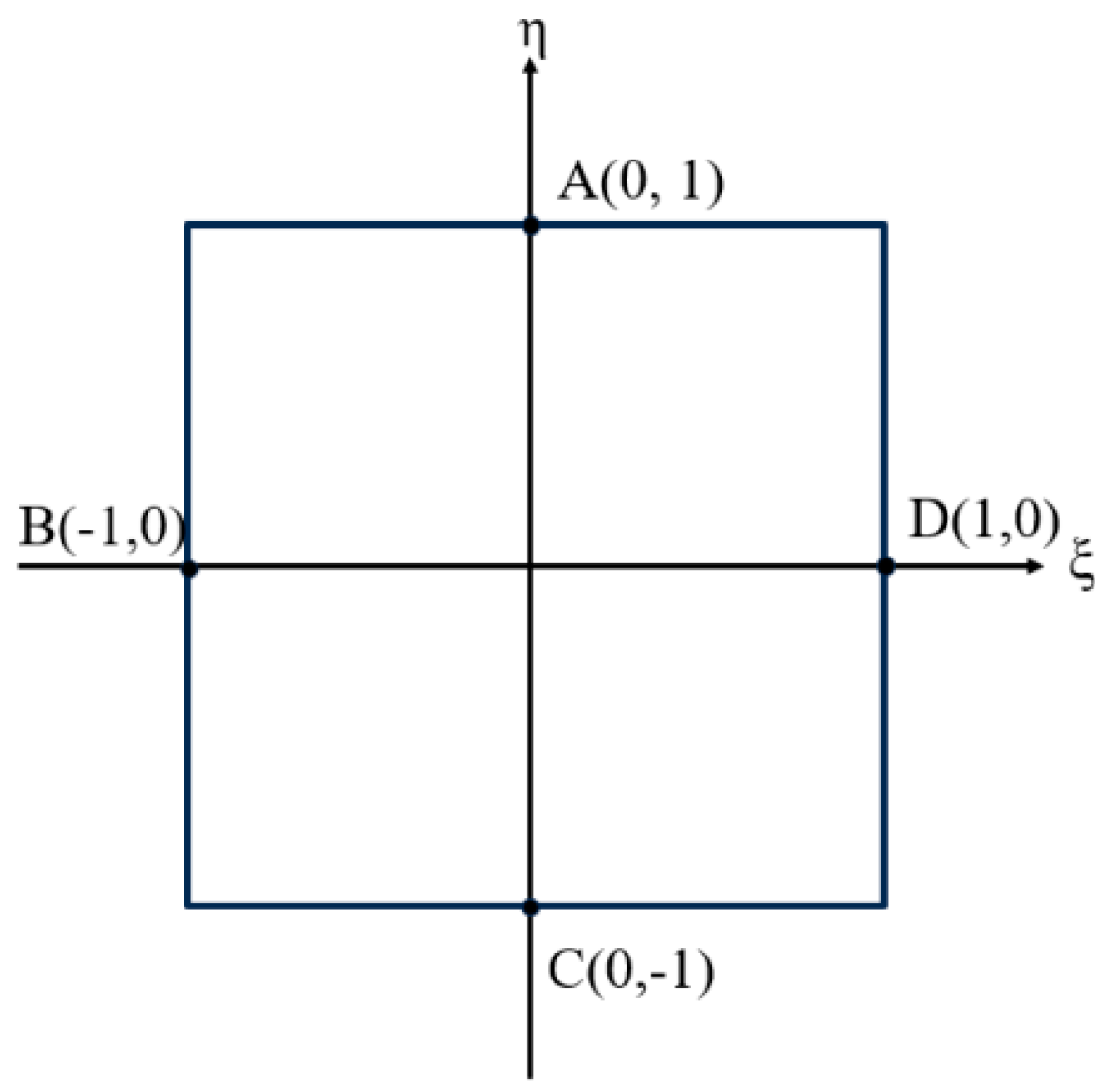
3. Assumed Strain Rate Interpolation

The four-node quadrilateral shell element can transform the node coordinates, node velocities, and angular velocities expressed in the global coordinate system into the unit coordinate system using the coordinate transformation matrix.

As shown in Figure 2, the origin of the cell coordinate system is located in the center of the cell $(x_c,y_x,z_c)$, and the vectors $g_1$ and $g_2$ are equal to

$$g_1=({\displaystyle \frac{\partial x}{\partial \xi }},{\displaystyle \frac{\partial y}{\partial \xi }},{\displaystyle \frac{\partial z}{\partial \xi }})$$

(11)

$$g_2=({\displaystyle \frac{\partial x}{\partial \eta }},{\displaystyle \frac{\partial y}{\partial \eta }},{\displaystyle \frac{\partial z}{\partial \eta }})$$

(12)

The base vectors $e_1$, $e_2$, and $e_3$ of the element coordinate system are determined as follows:

$$e_3={\displaystyle \frac{g_1\times g_2}{\left|g_1\times g_2\right|}}{\tilde{e}}_2={\displaystyle \frac{e_3\times g_1}{\left|e_3\times g_1\right|}}{e}_2={\displaystyle \frac{{\tilde{e}}_2+g_2/\left|g_2\right|}{\left|{\tilde{e}}_2+g_2/\left|g_2\right|\right|}}{e}_1={\displaystyle \frac{e_2\times e_3}{\left|e_2\times e_3\right|}}$$

(13)

Therefore, the vectors $e_1$, $e_2$, $g_1$, and $g_2$ are coplanar, and the angle between $e_1$ and $g_1$ is equal to the angle between $e_2$ and $g_2$. The coordinate transformation matrix $\lambda =\left[\begin{array}{ccc}{e}_1& e_2& e_3\end{array}\right]$ is then applied. Subsequently, the element node coordinates, node velocity, and angular velocity expressed in the global coordinate system are converted to the unit coordinate system.

$$\left[\begin{array}{c}{\widehat{x}}_I\\ {\widehat{y}}_I\\ {\widehat{z}}_I\end{array}\right]={\lambda }^{\mathrm{T}}\left[\begin{array}{c}{x}_I-x_C\\ y_I-y_C\\ z_I-z_C\end{array}\right]\left[\begin{array}{c}{\widehat{u}}_I\\ {\widehat{v}}_I\\ {\widehat{w}}_I\end{array}\right]={\lambda }^{\mathrm{T}}\left[\begin{array}{c}{u}_I\\ v_I\\ w_I\end{array}\right]\left[\begin{array}{c}{\widehat{\omega }}_{xI}\\ {\widehat{\omega }}_{yI}\\ {\widehat{\omega }}_{zI}\end{array}\right]={\lambda }^{\mathrm{T}}\left[\begin{array}{c}{\omega }_{xI}\\ {\omega }_{yI}\\ {\omega }_{zI}\end{array}\right]$$

(14)

where ${\left[\begin{array}{ccc}{x}_I-x_c& y_I-y_c& z_I-z_c\end{array}\right]}^T$ represents the relative coordinates relative to the center of the unit, ${\left[\begin{array}{ccc}{\widehat{x}}_I& {\widehat{y}}_I& {\widehat{z}}_I\end{array}\right]}^T$ represents the node coordinates in the unit coordinate system, ${\left[\begin{array}{ccc}{\widehat{u}}_I& {\widehat{v}}_I& {\widehat{w}}_I\end{array}\right]}^T$ represents the node velocity in the unit coordinate system, and ${\left[\begin{array}{ccc}{\widehat{\omega }}_{xI}& {\widehat{\omega }}_{yI}& {\widehat{\omega }}_{zI}\end{array}\right]}^T$ represents the node angular velocity in the unit coordinate system.

Symbols such as $x_I$, $u_I$, and ${\omega }_{Ix}$ indicate node coordinates, velocities, and angular velocities that have been transformed to the unit coordinate system.

The element coordinate system moves and rotates with the unit itself, so the element coordinate system is also a corotational coordinate system, and the objective stress rate is equivalent to the stress rate given by Jaumann [38]. When calculating the element, the strain rate can be divided into in-plane components and transverse shear components.

3.1. In-Plane Strainrate Interpolation

The membrane (in-plane) components of the rate-of-deformation tensor are given by

$${\dot{\epsilon }}_{ij}={\displaystyle \frac{1}{2}}\left({\displaystyle \frac{\partial V_i}{\partial x_j}}+{\displaystyle \frac{\partial V_j}{\partial x_i}}\right)$$

(15)

Substituting Equation (10) into Equation (15), we obtain

$${\dot{\epsilon }}_{xx}={\displaystyle \frac{\partial u}{\partial x}}=N_{I,x}(u_I+{\displaystyle \frac{a}{2}}\zeta {\omega }_{yI})+N_{I,x}^u{\omega }_{zI}$$

(16)

$${\dot{\epsilon }}_{yy}={\displaystyle \frac{\partial v}{\partial y}}=N_{I,y}(v_I-{\displaystyle \frac{a}{2}}\zeta {\omega }_{xI})+N_{I,y}^v{\omega }_{zI}$$

(17)

$${\dot{\epsilon }}_{xy}={\displaystyle \frac{\partial u}{\partial y}}+{\displaystyle \frac{\partial v}{\partial x}}=N_{I,y}(u_I+{\displaystyle \frac{a}{2}}\zeta {\omega }_{yI})+N_{I,x}(v_I-{\displaystyle \frac{a}{2}}\zeta {\omega }_{xI})+N_{I,y}^u{\omega }_{zI}+N_{I,x}^v{\omega }_{zI}$$

(18)

Writing Equations (16)–(18) in matrix form yields the following:

$$\dot{\epsilon }=\left[\begin{array}{c}{\dot{\epsilon }}_{xx}\\ {\dot{\epsilon }}_{yy}\\ {\dot{\epsilon }}_{xy}\end{array}\right]=\left[\begin{array}{cccccc}{N}_{I,x}& 0& 0& 0& {\displaystyle \frac{a}{2}}\zeta N_{I,x}& N_{I,x}^u\\ 0& N_{I,y}& 0& -{\displaystyle \frac{a}{2}}\zeta N_{I,y}& 0& N_{I,y}^v\\ N_{I,y}& N_{I,x}& 0& -{\displaystyle \frac{a}{2}}\zeta N_{I,x}& {\displaystyle \frac{a}{2}}\zeta N_{I,y}& N_{I,y}^u+N_{I,x}^v\end{array}\right]\left[\begin{array}{c}{u}_I\\ v_I\\ w_I\\ {\omega }_{xI}\\ {\omega }_{yI}\\ {\omega }_{zI}\end{array}\right]$$

(19)

The rate of deformation in Equation (19) can be written as the sum of the membrane and bending parts:

$$\dot{\epsilon }={\dot{\epsilon }}_m+{\dot{\epsilon }}_b=(B_I^m+B_I^b)U$$

(20)

where $v$ is a nodal velocity (translation and rotation) vector, $B_I^{\mathrm{m}}$ is a submatrix (block) of the membrane part of the gradient matrix, and $B_I^{\mathrm{b}}$ is the bending part:

$$B_I^{\mathrm{m}}=\left[\begin{array}{cccccc}{N}_{I,x}& 0& 0& 0& 0& N_{I,x}^u\\ 0& N_{I,y}& 0& 0& 0& N_{I,y}^v\\ N_{I,y}& N_{I,x}& 0& 0& 0& N_{I,y}^u+N_{I,x}^v\end{array}\right]$$

(21)

$$B_I^b={\displaystyle \frac{a}{2}}\zeta \left[\begin{array}{cccccc}0& 0& 0& 0& N_{I,x}& 0\\ 0& 0& 0& -N_{I,y}& 0& 0\\ 0& 0& 0& -N_{I,x}& N_{I,y}& 0\end{array}\right]$$

(22)

The derivatives of the shape functions with respect to the referential coordinates are

$$N_{I,\xi }={\displaystyle \frac{1}{4}}\left({\xi }_I+h_I\eta \right),N_{I,\eta }={\displaystyle \frac{1}{4}}\left({\eta }_I+h_I\xi \right)$$

(23)

where

$$\xi =\left[\begin{array}{cccc}1& -1& -1& 1\end{array}\right]$$

(24)

$$\eta =\left[\begin{array}{cccc}1& 1& -1& -1\end{array}\right]$$

(25)

Substituting the finite element interpolants in Equation (23) into the $2\times 2$ Jacobian matrix yields

$$J=\left[\begin{array}{cc}{\displaystyle \frac{\partial x}{\partial \xi }}& {\displaystyle \frac{\partial y}{\partial \xi }}\\ {\displaystyle \frac{\partial x}{\partial \eta }}& {\displaystyle \frac{\partial y}{\partial \eta }}\end{array}\right]=\left[\begin{array}{cc}{\displaystyle \frac{1}{4}}({\xi }_I+h_I\eta )x_I& {\displaystyle \frac{1}{4}}({\xi }_I+h_I\eta )y_I\\ {\displaystyle \frac{1}{4}}\left({\eta }_I+h_I\xi \right)x_I& {\displaystyle \frac{1}{4}}\left({\eta }_I+h_I\xi \right)y_I\end{array}\right]$$

(26)

The determinant J of the $2\times 2$ Jacobian matrix can be expressed as

$$J=\left|J\right|=J_0+J_1\xi +J_2\eta$$

(27)

where

$$\begin{array}{l}{J}_0={\displaystyle \frac{1}{16}}\left[\left({\xi }_I{x}_I\right)\left({\eta }_J{y}_J\right)-\left({\eta }_I{x}_I\right)\left({\xi }_J{y}_J\right)\right]\\ J_1={\displaystyle \frac{1}{16}}\left[\left({\xi }_I{x}_I\right)\left(h_J{y}_J\right)-\left(h_I{x}_I\right)\left({\xi }_J{y}_J\right)\right]\\ J_2={\displaystyle \frac{1}{16}}\left[\left(h_I{x}_I\right)\left({\eta }_J{y}_J\right)-\left({\eta }_I{x}_I\right)\left(h_J{y}_J\right)\right]\end{array}$$

(28)

It is useful to write the shape functions in an equivalent manner:

$$N_I=\Delta +x{b}_x+y{b}_y+h\gamma$$

(29)

where

$${\Delta }_I={\displaystyle \frac{1}{4}}\left[t_I-(t_J{x}_J)b_{xI}-(t_J{y}_J)b_{yI}\right],b_{xI}={\displaystyle \frac{1}{2A}}[\begin{array}{cccc}{\widehat{y}}_{24}& {\widehat{y}}_{31}& {\widehat{y}}_{42}& {\widehat{y}}_{13}\end{array}]$$

(30)

$$b_{yI}={\displaystyle \frac{1}{2A}}[\begin{array}{cccc}{\widehat{x}}_{42}& {\widehat{x}}_{13}& {\widehat{x}}_{24}& {\widehat{x}}_{31}\end{array}],{\gamma }_I={\displaystyle \frac{1}{4}}\left[h_I-(h_J{x}_J)b_{xI}-(h_J{y}_J)b_{yI}\right],$$

(31)

$$x_{IJ}=x_I-x_J,y_{IJ}=y_I-y_J$$

(32)

$$t_I=\left[\begin{array}{cccc}1& 1& 1& 1\end{array}\right],h_I=\left[\begin{array}{cccc}1& -1& 1& -1\end{array}\right],h=\xi \eta$$

(33)

where A is the area of the element. For a warped element, A is the area projected onto the x-y plane.

Belytschko [39,40] demonstrates that, when rigid body rotation occurs in a warped element, the unsteady components of both the membrane strain and bending strain within the element do not vanish.

$$B_I^{\mathrm{m}}=\left[\begin{array}{cccccc}{N}_{I,x}& 0& 0& 0& -0.25z_{\gamma }{h}_{,x}& N_{I,x}^u\\ 0& N_{I,y}& 0& 0.25z_{\gamma }{h}_{,y}& 0& N_{I,y}^v\\ N_{I,y}& N_{I,x}& 0& 0.25z_{\gamma }{h}_{,x}& 0.25z_{\gamma }{h}_{,y}& N_{I,y}^u+N_{I,x}^v\end{array}\right]$$

(34)

$$B_I^b={\displaystyle \frac{a}{2}}\zeta \left[\begin{array}{cccccc}{b}_x^{\mathrm{c}I}& 0& 0& 0& N_{I,x}& 0\\ 0& b_y^{\mathrm{c}I}& 0& -N_{I,y}& 0& 0\\ b_y^{\mathrm{c}I}& b_x^{\mathrm{c}I}& 0& -N_{I,x}& N_{I,y}& 0\end{array}\right]$$

(35)

where

$$h_{,x}={\displaystyle \frac{1}{4J}}\left[({\eta }_I{y}_I)\eta -({\xi }_I{y}_I)\xi \right],h_{,y}={\displaystyle \frac{1}{4J}}\left[({\xi }_I{x}_I)\xi -({\eta }_I{y}_I)\eta \right]$$

(36)

$$z_{\gamma }={\displaystyle \sum _{I=1}^4{z}_I{\gamma }_I}$$

(37)

$$b_x^{\mathrm{c}}={\displaystyle \frac{4z_{\gamma }}{A}}\left[\begin{array}{cccc}{b}_{y2}& b_{y1}& b_{y4}& b_{y3}\end{array}\right]$$

(38)

$$b_y^{\mathrm{c}}={\displaystyle \frac{4z_{\gamma }}{A}}\left[\begin{array}{cccc}{b}_{x4}& b_{x3}& b_{x2}& b_{x1}\end{array}\right]$$

(39)

3.2. Transverse Shear–Velocity–Strain Interpolation

According to Bathe [23], the nodes in the quadrilateral are interpolated within the natural coordinate system, with the covariant components represented by tensors. The covariant components in the unit coordinate system are derived following a transformation. The transverse shear strain rate is expressed through the covariant component in the element coordinate system.

In the rectangular coordinate system (xyz), the relationship between the covariant component of the velocity gradient $L_{ij}$ in the xyz system and the covariant component ${\tilde{L}}_{ij}$ in the $\xi \eta \zeta$ system is established:

$${\tilde{L}}_{ij}={\beta }_i^m{\beta }_j^n{L}_{mn}={\displaystyle \frac{\partial x^m}{\partial {\xi }^i}}{\displaystyle \frac{\partial x^n}{\partial {\xi }^j}}{\displaystyle \frac{\partial v_m}{\partial x^n}}={\displaystyle \frac{\partial x^m}{\partial {\xi }^i}}{\displaystyle \frac{\partial v_m}{\partial {\xi }^j}}$$

(40)

where $v_i=\left[\begin{array}{ccc}u& v& w\end{array}\right]$, $x^i=\left[\begin{array}{ccc}x& y& z\end{array}\right]$, ${\xi }^i=\left[\begin{array}{ccc}\xi & \eta & \zeta \end{array}\right]$.

In the $\xi \eta \zeta$ coordinate system, the velocity gradient components ${\tilde{L}}_{\xi \zeta }$, ${\tilde{L}}_{\zeta \xi }$, ${\tilde{L}}_{\eta \zeta }$, and ${\tilde{L}}_{\zeta \eta }$ are

$$\begin{array}{l}{\tilde{L}}_{\xi \zeta }={\displaystyle \frac{\partial x^m}{\partial \xi }}{\displaystyle \frac{\partial v_m}{\partial \zeta }}=J_{11}{\displaystyle \frac{\partial u}{\partial \zeta }}+J_{12}{\displaystyle \frac{\partial v}{\partial \zeta }}+J_{13}{\displaystyle \frac{\partial w}{\partial \zeta }}\\ {\tilde{L}}_{\zeta \xi }={\displaystyle \frac{\partial x^m}{\partial \zeta }}{\displaystyle \frac{\partial v_m}{\partial \xi }}=J_{31}{\displaystyle \frac{\partial u}{\partial \xi }}+J_{32}{\displaystyle \frac{\partial v}{\partial \xi }}+J_{33}{\displaystyle \frac{\partial w}{\partial \xi }}\\ {\tilde{L}}_{\eta \zeta }={\displaystyle \frac{\partial x^m}{\partial \eta }}{\displaystyle \frac{\partial v_m}{\partial \zeta }}=J_{21}{\displaystyle \frac{\partial u}{\partial \zeta }}+J_{22}{\displaystyle \frac{\partial v}{\partial \zeta }}+J_{23}{\displaystyle \frac{\partial w}{\partial \zeta }}\\ {\tilde{L}}_{\zeta \eta }={\displaystyle \frac{\partial x^m}{\partial \zeta }}{\displaystyle \frac{\partial v_m}{\partial \eta }}=J_{31}{\displaystyle \frac{\partial u}{\partial \eta }}+J_{32}{\displaystyle \frac{\partial v}{\partial \eta }}+J_{33}{\displaystyle \frac{\partial w}{\partial \eta }}\end{array}$$

(41)

where $J_{ij}={\displaystyle \frac{\partial x^i}{\partial {\xi }^j}}$ is a term in the 3 × 3 Jacobian matrix. We ignore terms containing $J_{13}$,$J_{23}$, $J_{31}$, and $J_{32}$, and take $J_{33}\cong {\displaystyle \frac{a}{2}}$. Substituting Equations (14) and (15) into Equation (41), we obtain

$$\begin{array}{l}{\tilde{L}}_{\xi \zeta }=0.5a[J_{11}{N}_I{\omega }_{yI}-J_{12}{N}_I{\omega }_{xI}]{\tilde{L}}_{\zeta \xi }=0.5a{N}_{I,\xi }{w}_I\\ {\tilde{L}}_{\eta \zeta }=0.5a[J_{21}{N}_I{\omega }_{yI}-J_{22}{N}_I{\omega }_{xI}]{\tilde{L}}_{\zeta \eta }=0.5a{N}_{I,\eta }{w}_I\end{array}$$

(42)

In Figure 3, the A point coordinates in the natural coordinate system of $(0,1,0)$ and the C point coordinates in the natural coordinate system of $(0,-1,0)$ are shown. In this case, we obtain

$$\begin{array}{l}{\tilde{L}}_{\xi \zeta }^A=0.5a[J_{11}^A{N}_I^A{\omega }_{yI}-J_{12}^A{N}_I^A{\omega }_{xI}]\\ {\tilde{L}}_{\zeta \xi }^A=0.5a{N}_{I,\xi }^A{w}_I\end{array}$$

(43)

$$\begin{array}{l}{\tilde{L}}_{\eta \zeta }^C=0.5a[J_{11}^C{N}_I^C{\omega }_{yI}-J_{12}^C{N}_I^C{\omega }_{xI}]\\ L_{\zeta \eta }^C=0.5a{N}_{I,\eta }^C{w}_I\end{array}$$

(44)

The distribution of ${\tilde{L}}_{\xi \zeta }$ and ${\tilde{L}}_{\zeta \xi }$ in the element is

$${\tilde{L}}_{\xi \zeta }={\displaystyle \frac{1}{2}}{\tilde{L}}_{\xi \zeta }^A(1+\eta )+{\displaystyle \frac{1}{2}}{\tilde{L}}_{\xi \zeta }^C(1-\eta )=0.5a{\mathrm{S}}_{12}^{AC}{\omega }_{xI}+0.5h{\mathrm{S}}_{11}^{AC}{\omega }_{yI}$$

(45)

$${\tilde{L}}_{\zeta \xi }={\displaystyle \frac{1}{2}}{\tilde{L}}_{\zeta \xi }^A(1+\eta )+{\displaystyle \frac{1}{2}}{\tilde{L}}_{\zeta \xi }^C(1-\eta )=0.5h{\mathrm{S}}_{,\xi }^{AC}{w}_I$$

(46)

where

$$\begin{array}{l}{S}_{12}^{AC}=-0.5J_{12}^A{N}_I^A(1+\eta )-0.5J_{12}^C{N}_I^C(1-\eta )\\ {\mathrm{S}}_{11}^{AC}=0.5J_{11}^A{N}_I^A(1+\eta )+0.5J_{11}^C{N}_I^C(1-\eta )\\ {\mathrm{S}}_{,r}^{AC}=0.5N_{I,\xi }^A(1+\eta )+0.5N_{I,\xi }^C(1-\eta )\end{array}$$

(47)

Similarly, the distribution of ${\tilde{L}}_{\eta \zeta }$ and ${\tilde{L}}_{\zeta \eta }$ in the element is

$${\tilde{L}}_{\eta \zeta }={\displaystyle \frac{1}{2}}{\tilde{L}}_{\eta \zeta }^B(1-\xi )+{\displaystyle \frac{1}{2}}{\tilde{L}}_{\eta \zeta }^D(1+\xi )=0.5a{\mathrm{R}}_{22}^{BD}{\omega }_{xI}+0.5a{\mathrm{R}}_{21}^{BD}{\omega }_{yI}$$

(48)

$${\tilde{L}}_{\zeta \eta }={\displaystyle \frac{1}{2}}{\tilde{L}}_{\zeta \eta }^B(1-\xi )+{\displaystyle \frac{1}{2}}{\tilde{L}}_{\zeta \eta }^D(1+\xi )=0.5a{\mathrm{R}}_{,\eta }^{BD}{w}_I$$

(49)

where

$$\begin{array}{l}{\mathrm{R}}_{22}^{BD}=-0.5J_{22}^B{N}_I^B(1-\xi )-0.5J_{22}^D{N}_I^D(1+\xi )\\ {\mathrm{R}}_{21}^{BD}=0.5J_{21}^B{N}_I^B(1-\xi )+0.5J_{21}^D{N}_I^D(1+\xi )\\ {\mathrm{R}}_{,\eta }^{BD}=0.5N_{I,\eta }^B(1-\xi )+0.5N_{I,\eta }^D(1+\xi )\end{array}$$

(50)

The covariant component of the velocity gradient L within the xyz coordinate system can also be represented by its corresponding covariant component in another $\xi \eta \zeta$ coordinate system.

$$\begin{array}{c}{L}_{xz}={\displaystyle \frac{\partial \xi }{\partial x}}{\displaystyle \frac{\partial \xi }{\partial z}}{\tilde{L}}_{\xi \xi }+{\displaystyle \frac{\partial \xi }{\partial x}}{\displaystyle \frac{\partial \eta }{\partial z}}{\tilde{L}}_{\xi \eta }+{\displaystyle \frac{\partial \xi }{\partial x}}{\displaystyle \frac{\partial \zeta }{\partial z}}{\tilde{L}}_{\xi \zeta }+{\displaystyle \frac{\partial \eta }{\partial x}}{\displaystyle \frac{\partial \xi }{\partial z}}{\tilde{L}}_{\eta \xi }+{\displaystyle \frac{\partial \eta }{\partial x}}{\displaystyle \frac{\partial \eta }{\partial z}}{\tilde{L}}_{\eta \eta }\\ +{\displaystyle \frac{\partial \eta }{\partial x}}{\displaystyle \frac{\partial \zeta }{\partial z}}{\tilde{L}}_{\eta \zeta }+{\displaystyle \frac{\partial \zeta }{\partial x}}{\displaystyle \frac{\partial \xi }{\partial z}}{\tilde{L}}_{\zeta \xi }+{\displaystyle \frac{\partial \zeta }{\partial x}}{\displaystyle \frac{\partial \eta }{\partial z}}{\tilde{L}}_{\zeta \eta }+{\displaystyle \frac{\partial \zeta }{\partial x}}{\displaystyle \frac{\partial \zeta }{\partial z}}{\tilde{L}}_{\zeta \zeta }\\ L_{zx}={\displaystyle \frac{\partial \xi }{\partial z}}{\displaystyle \frac{\partial \xi }{\partial x}}{\tilde{L}}_{\xi \xi }+{\displaystyle \frac{\partial \xi }{\partial z}}{\displaystyle \frac{\partial \eta }{\partial x}}{\tilde{L}}_{\xi \eta }+{\displaystyle \frac{\partial \xi }{\partial z}}{\displaystyle \frac{\partial \zeta }{\partial x}}{\tilde{L}}_{\xi \zeta }+{\displaystyle \frac{\partial \eta }{\partial z}}{\displaystyle \frac{\partial \xi }{\partial x}}{\tilde{L}}_{\eta \xi }+{\displaystyle \frac{\partial \eta }{\partial z}}{\displaystyle \frac{\partial \eta }{\partial x}}{\tilde{L}}_{\eta \eta }\\ +{\displaystyle \frac{\partial \eta }{\partial z}}{\displaystyle \frac{\partial \zeta }{\partial x}}{\tilde{L}}_{\eta \zeta }+{\displaystyle \frac{\partial \zeta }{\partial z}}{\displaystyle \frac{\partial \xi }{\partial x}}{\tilde{L}}_{\zeta \xi }+{\displaystyle \frac{\partial \zeta }{\partial z}}{\displaystyle \frac{\partial \eta }{\partial x}}{\tilde{L}}_{\zeta \eta }+{\displaystyle \frac{\partial \zeta }{\partial z}}{\displaystyle \frac{\partial \zeta }{\partial x}}{\tilde{L}}_{\zeta \zeta }\end{array}$$

(51)

where $\partial \xi /\partial z=\partial \eta /\partial z=0$ and $\partial \zeta /\partial z=2/\mathrm{a}$. Additionally, for the element, since the $\xi \eta$ plane is parallel to the xy plane and $\zeta$ is perpendicular to the z direction, ${\tilde{L}}_{\zeta \zeta }=0$.

$$\begin{array}{l}{L}_{xz}={\displaystyle \frac{2}{a}}(J_{11}^{-1}{\tilde{L}}_{\xi \zeta }+J_{12}^{-1}{\tilde{L}}_{\eta \zeta })=J_{11}^{-1}{\mathrm{S}}_{12}^{AC}{\omega }_{xI}+J_{12}^{-1}{\mathrm{R}}_{22}^{BD}{\omega }_{xI}+J_{11}^{-1}{\mathrm{S}}_{11}^{AC}{\omega }_{yI}+J_{12}^{-1}{\mathrm{R}}_{21}^{BD}{\omega }_{yI}\\ L_{zx}={\displaystyle \frac{2}{a}}(J_{11}^{-1}{\tilde{L}}_{\zeta \xi }+J_{12}^{-1}{\tilde{L}}_{\zeta \eta })=J_{11}^{-1}{\mathrm{S}}_{,\xi }^{AC}{w}_I+J_{12}^{-1}{\mathrm{R}}_{,\eta }^{BD}{w}_I\end{array}$$

(52)

For the covariant components $L_{yz}$ and $L_{zy}$, we have the same:

$$\begin{array}{l}{L}_{yz}={\displaystyle \frac{2}{a}}(J_{21}^{-1}{\tilde{L}}_{\xi t}+J_{22}^{-1}{\tilde{L}}_{\eta \zeta })=J_{21}^{-1}{\mathrm{S}}_{12}^{AC}{\omega }_{xI}+J_{22}^{-1}{\mathrm{R}}_{22}^{BD}{\omega }_{xI}+J_{21}^{-1}{\mathrm{S}}_{11}^{AC}{\omega }_{yI}+J_{22}^{-1}{\mathrm{R}}_{21}^{BD}{\omega }_{yI}\\ L_{zy}={\displaystyle \frac{2}{a}}(J_{21}^{-1}{\tilde{L}}_{\zeta \eta }+J_{22}^{-1}{\tilde{L}}_{\zeta \eta })=J_{21}^{-1}{\mathrm{S}}_{,\xi }^{AC}{w}_I+J_{22}^{-1}{\mathrm{R}}_{,\eta }^{BD}{w}_I\end{array}$$

(53)

The $B_I^s$ matrix corresponding to the transverse shear strain rates ${\dot{\epsilon }}_{yz}$ and ${\dot{\epsilon }}_{zx}$ is obtained:

$$\left[\begin{array}{c}{\dot{\epsilon }}_{yz}\\ {\dot{\epsilon }}_{zx}\end{array}\right]=\left[\begin{array}{c}{L}_{yz}+L_{zy}\\ L_{xz}+L_{zx}\end{array}\right]=B_I^s\left[\begin{array}{c}{w}_I\\ {\omega }_{xI}\\ {\omega }_{yI}\end{array}\right]$$

(54)

where

$$B_{\mathrm{I}}^s=\left[\begin{array}{ccc}{J}_{21}^{-1}{\mathrm{S}}_{,\xi }^{AC}+J_{22}^{-1}{\mathrm{R}}_{,\eta }^{BD}& J_{21}^{-1}{\mathrm{S}}_{12}^{AC}+J_{22}^{-1}{\mathrm{R}}_{22}^{BD}& J_{21}^{-1}{\mathrm{S}}_{11}^{AC}+J_{22}^{-1}{\mathrm{R}}_{21}^{BD}\\ J_{11}^{-1}{\mathrm{S}}_{,\xi }^{AC}+J_{12}^{-1}{\mathrm{R}}_{,\eta }^{BD}& J_{11}^{-1}{\mathrm{S}}_{12}^{AC}+J_{12}^{-1}{\mathrm{R}}_{22}^{BD}& J_{11}^{-1}{\mathrm{S}}_{11}^{AC}+J_{12}^{-1}{\mathrm{R}}_{21}^{BD}\end{array}\right]$$

(55)

3.3. Elimination of Corotational Zero-Energy Mode

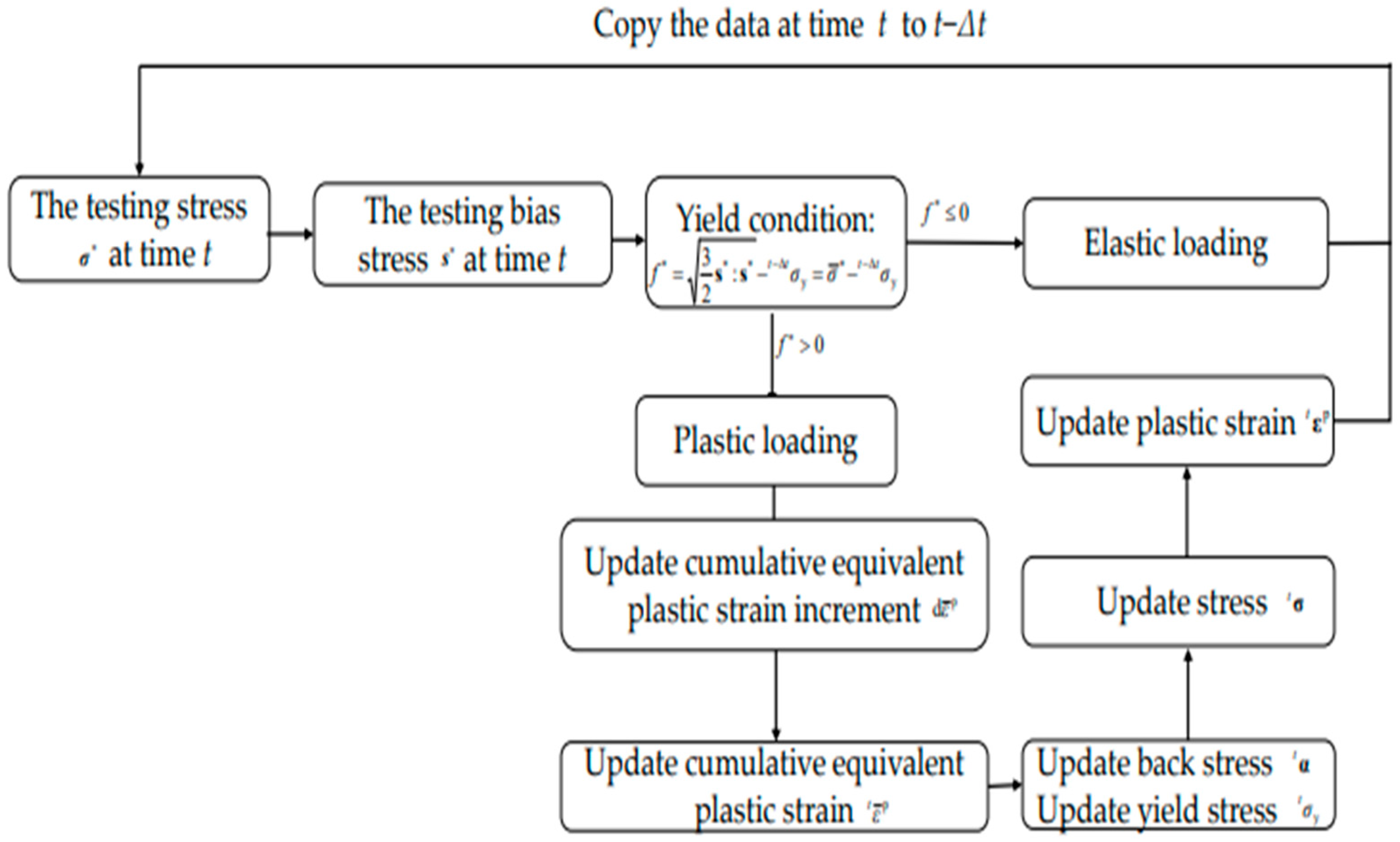
The introduction of additional stiffness eliminates the zero-energy mode that arises when degrees of freedom around the normal are incorporated into the quadrilateral shell element. The minimum rotation calculated in the displacement interpolation mode at the center of the element is as follows:

$$\Omega {|}_{\xi ,\eta =0}={\displaystyle \frac{1}{2}}({\displaystyle \frac{\partial v}{\partial x}}-{\displaystyle \frac{\partial u}{\partial y}})=B^{\Omega }{U}_e$$

(56)

where $U_e={\left[\begin{array}{ccc}{u}_I& v_I& {\omega }_{ZI}\end{array}\right]}^T$, and the submatrix $B_I^{\Omega }$ of transverse shear strain rate $B^{\Omega }$ is

$$B_I^{\Omega }={\displaystyle \frac{1}{2}}\left[\begin{array}{ccc}-{\displaystyle \frac{\partial N_I}{\partial y}}& {\displaystyle \frac{\partial N_I}{\partial x}}& -{\displaystyle \frac{\partial N_I^u}{\partial y}}+{\displaystyle \frac{\partial N_I^v}{\partial x}}\end{array}\right]$$

(57)

The degree of freedom of node rotation is interpolated at the origin of the element coordinates:

$$\omega {|}_{\xi ,\eta =0}={\overline{B}}^{\omega }{U}_e,{\overline{B}}_I^{\omega }=\left[\begin{array}{ccc}0& 0& 0.25\end{array}\right]$$

(58)

We introduce the constraint $\Omega {|}_{\xi ,\eta =0}=\omega {|}_{\xi ,\eta =0}$ at the origin of the element coordinates,

$$\left(B^{\Omega }-{\overline{B}}^{\omega }\right)U_e=0$$

(59)

Using the penalty function to deal with constraints, the corresponding equal effect is

$$F^{\mathrm{penalty}}=\gamma aG{\displaystyle \underset{A}{\iint }{\left(B^{\Omega }-{\overline{B}}^{\omega }\right)}^{\mathrm{T}}\left(B^{\Omega }-{\overline{B}}^{\omega }\right)\mathrm{d}A}$$

(60)

where A is the area of the element, a is the thickness of the unit, G is the shear modulus, and $\gamma$ is the penalty factor. According to MacNeal [21], the penalty factor takes a value of ${10}^{-6}$.

4. Plastic Analysis

The deformation rate tensor $\dot{\epsilon }$ is decomposed into the elastic ${\dot{\epsilon }}^{\mathrm{e}}$ and plastic ${\dot{\epsilon }}^{\mathrm{p}}$ parts:

$$\dot{\epsilon }={\dot{\epsilon }}^{\mathrm{e}}+{\dot{\epsilon }}^{\mathrm{p}}$$

(61)

Let ${\sigma }_{ij}$ be the stress tensor, ${\alpha }_{ij}$ be the back stress tensor, and $s_{ij}$ be the deflection stress tensor after taking into account the back stress, i.e.,

$$s_{ij}={\sigma }_{ij}-{\alpha }_{ij}-{\delta }_{ij}({\sigma }_{mm}-{\alpha }_{mm})/3$$

(62)

where ${\delta }_{\mathrm{ij}}$ is the Kronecker delta. For ideal elastoplastic or isotropic hardening, the back stress ${\alpha }_{ij}=0$.

In $J_2$ flow theory, the equivalent stress $\overline{\sigma }$ is defined as a function of the second invariant $J_2$ of the tensor $s_{ij}$:

$$\overline{\sigma }=\sqrt{3J_2}=\sqrt{1.5s_{ij}{s}_{ij}}$$

(63)

The yield condition is

$$f=\sqrt{3J_2}-{\sigma }_{\mathrm{y}}({\overline{\epsilon }}^{\mathrm{p}})=\overline{\sigma }-{\sigma }_{\mathrm{y}}({\overline{\epsilon }}^{\mathrm{p}})=0$$

(64)

where ${\sigma }_{\mathrm{y}}({\overline{\epsilon }}^{\mathrm{p}})$ represents the yield stress of the material, which typically depends on the internal variable ${\overline{\epsilon }}^{\mathrm{p}}={\displaystyle \int \mathrm{d}{\overline{\epsilon }}^{\mathrm{p}}}$. $\mathrm{d}{\overline{\epsilon }}^{\mathrm{p}}$ denotes the increment in the equivalent plastic strain. $f<0$ corresponds to elasticity and $f=0$ represents cumulative equivalent plastic anisotropy.

The ideal elastic–plastic models, isotropic hardening, kinematic hardening, and mixed hardening can be expressed in a unified form by assuming a linear relationship between ${\sigma }_{\mathrm{y}}({\overline{\epsilon }}^{\mathrm{p}})$ and ${\sigma }_{\mathrm{y}}({\overline{\epsilon }}^{\mathrm{p}})$ (i.e., linear strengthening). Additionally, a parameter $\beta$ is introduced to facilitate this relationship.

$${\sigma }_{\mathrm{y}}={\sigma }_{\mathrm{y}0}+\beta E_{\mathrm{p}}{\overline{\epsilon }}^{\mathrm{p}}$$

(65)

$${\alpha }_{ij}^{\nabla \mathrm{J}}={\displaystyle \frac{2}{3}}(1-\beta )E_{\mathrm{p}}{\dot{\epsilon }}_{ij}^{\mathrm{p}}$$

(66)

where $E_{\mathrm{p}}=\mathrm{d}{\sigma }_{\mathrm{y}}/\mathrm{d}{\overline{\epsilon }}^{\mathrm{p}}=0$ is the ideal elastoplastic case; if $E_{\mathrm{p}}\ne 0$, $\beta =1$ corresponds to isotropic hardening; if $E_{\mathrm{p}}\ne 0$, $\beta =0$ corresponds to kinematic hardening; if $E_{\mathrm{p}}\ne 0$, $\beta \in (0,1)$ corresponds to mixed hardening.

According to the correlated plastic flow law, the plastic part of the deformation rate tensor $\dot{\epsilon }$ is

$${\dot{\epsilon }}_{ij}^{\mathrm{p}}=\dot{\lambda }{\displaystyle \frac{\partial f}{\partial {\sigma }_{ij}}}={\displaystyle \frac{\dot{\lambda }}{2}}\sqrt{{\displaystyle \frac{3}{J_2}}}{\displaystyle \frac{\partial J_2}{\partial {\sigma }_{ij}}}={\displaystyle \frac{3s_{ij}}{2\overline{\sigma }}}\dot{\lambda }$$

(67)

where $\dot{\lambda }$ is the scalar plastic flow rate. The Von Mises equivalent plastic deformation rate ${\dot{\overline{\epsilon }}}^{\mathrm{p}}$ is defined as

$${\dot{\overline{\epsilon }}}^{\mathrm{p}}={\left({\displaystyle \frac{2}{3}}{\dot{\epsilon }}_{ij}^{\mathrm{p}}{\dot{\epsilon }}_{ij}^{\mathrm{p}}\right)}^{0.5}={\displaystyle \frac{\dot{\lambda }}{\overline{\sigma }}}{\left({\displaystyle \frac{3s_{ij}{s}_{ij}}{2}}\right)}^{0.5}=\dot{\lambda }$$

(68)

The Jaumann rate ${\alpha }_{ij}^{\nabla J}$ of the back stress is obtained:

$${\alpha }_{ij}^{\nabla \mathrm{J}}={\displaystyle \frac{2}{3}}(1-\beta )E_{\mathrm{p}}{\dot{\epsilon }}_{ij}^{\mathrm{p}}={\displaystyle \frac{2}{3}}(1-\beta )E_{\mathrm{p}}{\displaystyle \frac{3s_{ij}}{2\overline{\sigma }}}\dot{\lambda }=(1-\beta )E_{\mathrm{p}}{\displaystyle \frac{s_{ij}}{\overline{\sigma }}}\dot{\lambda }$$

(69)

In the plastic analysis modeling program, the process is shown in Figure 4. From the displacement and velocity at time t, the deformation rate ^t$\dot{\epsilon }$ and the spin tensor ${}^t\Omega$ corresponding to time t can be obtained, and the testing stress ${\sigma }^{\ast }$ at time t can be determined:

$${}^t\sigma ^{\nabla \mathrm{J}}=C:{}^t\dot{\epsilon }$$

(70)

$${\sigma }^{\ast }={}^{t-\Delta t}\sigma +({\sigma }^{\nabla \mathrm{J}}-{}^{t-\Delta \mathrm{t}}\sigma \cdot {}^t\Omega +{}^t\Omega \cdot {}^{t-\Delta \mathrm{t}}\sigma )\Delta t$$

(71)

Moreover, the testing bias stress $s^{\ast }$ at time t is

$$s^{\ast }={\sigma }^{\ast }-{}^{t-\Delta t}\alpha -{\displaystyle \frac{1}{3}}({\sigma }_{kk}^{\ast }-{}^{t-\Delta t}\alpha _{kk})I$$

(72)

According to the yield conditions, we can determine whether the time t is in yield:

$$f^{\ast }=\sqrt{{\displaystyle \frac{3}{2}}{s}^{\ast }:s^{\ast }}-{}^{t-\Delta t}\sigma _{\mathrm{y}}={\overline{\sigma }}^{\ast }-{}^{t-\Delta t}\sigma _{\mathrm{y}}$$

(73)

where ${\overline{\sigma }}^{\ast }$ is the equivalent stress corresponding to the test stress. If $f^{\ast }\le 0$, then time t has an elastic or neutral variable load, where ^t$\sigma ={\sigma }^{\ast }$, and the plastic data at time $t-\Delta t$ are copied to time $t$. If $f^{\ast }>0$, time t is in a state of plastic loading. According to Equation (67), we obtain

$${\dot{\epsilon }}^{\mathrm{p}}=\dot{\lambda }{\displaystyle \frac{3}{2}}{\displaystyle \frac{{}^{t}s}{{}^t\overline{\sigma }}}=\dot{\lambda }{\displaystyle \frac{3}{2}}{\displaystyle \frac{s^{\ast }}{{\overline{\sigma }}^{\ast }}}$$

(74)

To ensure that the stress state at time t aligns with the yield surface at the same time, the test deviatoric stress $s^{\ast }$ is adjusted accordingly:

$${}^{t}s=s^{\ast }-2G{\dot{\epsilon }}^{\mathrm{p}}\mathrm{d}t=s^{\ast }-3G{\displaystyle \frac{s^{\ast }}{{\overline{\sigma }}^{\ast }}}\mathrm{d}\lambda$$

(75)

where we multiply both sides by ${\displaystyle \frac{3}{2}}{\displaystyle \frac{{}^{t}s}{{}^t\overline{\sigma }}}={\displaystyle \frac{3}{2}}{\displaystyle \frac{s^{\ast }}{{\overline{\sigma }}^{\ast }}}$ and notice that the formula ${}^t\overline{\sigma }_2=1.5{}^{t}s:{}^{t}s$.

$${}^t\overline{\sigma }={\overline{\sigma }}^{\ast }-3G\mathrm{d}\lambda ={\overline{\sigma }}^{\ast }-3G\mathrm{d}{\overline{\epsilon }}^{\mathrm{p}}$$

(76)

This illustrates the relationship between ${}^t\overline{\sigma }$, ${\overline{\sigma }}^{\ast }$, and $\mathrm{d}{\overline{\epsilon }}^{\mathrm{p}}$. For linear reinforcement, where ${\sigma }_{\mathrm{y}}$ is linear to ${\overline{\epsilon }}^{\mathrm{p}}$, $\mathrm{d}{\overline{\epsilon }}^{\mathrm{p}}$ can be calculated using the t time yield function.

$${}^{t}f={}^t\overline{\sigma }-{}^t\sigma _{\mathrm{y}}={\overline{\sigma }}^{\ast }-3G\mathrm{d}{\overline{\epsilon }}^{\mathrm{p}}-{}^{t-\Delta t}\sigma _y-\beta E_{\mathrm{p}}\mathrm{d}{\overline{\epsilon }}^{\mathrm{p}}$$

(77)

Thus, $\mathrm{d}{\overline{\epsilon }}^{\mathrm{p}}$ and ${}^t\overline{\epsilon }_{\mathrm{p}}$ are obtained:

$$\mathrm{d}{\overline{\epsilon }}^{\mathrm{p}}={\displaystyle \frac{{\overline{\sigma }}^{\ast }-{}^{t-\Delta t}\sigma _{\mathrm{y}}}{3G+E_{\mathrm{p}}}}$$

(78)

$${}^t\overline{\epsilon }^{\mathrm{p}}={}^{t-\Delta t}\overline{\epsilon }^{\mathrm{p}}+\mathrm{d}{\overline{\epsilon }}^{\mathrm{p}}$$

(79)

Bringing $\mathrm{d}{\overline{\epsilon }}^{\mathrm{p}}$ into Equation (75), again using the condition ${}^{t}s/{}^t\overline{\sigma }=s^{\ast }/{\overline{\sigma }}^{\ast }$, we have

$${}^{t}s=s^{\ast }-3G\mathrm{d}{\overline{\epsilon }}^{\mathrm{p}}{\displaystyle \frac{{}^t\mathit{s}}{{}^t\overline{\sigma }}}$$

(80)

This is a linear equation for ${}^{t}s$. By substituting Equation (78) into Equation (80), and noting that, at time t ^t$\overline{\sigma }={}^t\sigma _{\mathrm{y}}$, we obtain

$${}^{t}s={\displaystyle \frac{{}^t\overline{\sigma }}{{}^t\overline{\sigma }+3G\mathrm{d}{\overline{\epsilon }}^{\mathrm{p}}}}{s}^{\ast }={\displaystyle \frac{{}^t\overline{\sigma }}{{\overline{\sigma }}^{\ast }}}{s}^{\ast }={\displaystyle \frac{{}^t\sigma _{\mathrm{y}}}{{\overline{\sigma }}^{\ast }}}{s}^{\ast }$$

(81)

It can be observed that Equation (82) aims to reduce the testing deviant stress ${\overline{s}}^{\ast }$ in order to return it to the yield surface at time t. Therefore, for the stress update calculation,

$${}^t\sigma ={\sigma }^{\ast }-3G\mathrm{d}{\overline{\epsilon }}^{\mathrm{p}}{\displaystyle \frac{s^{\ast }}{{\overline{\sigma }}^{\ast }}}$$

(82)

5. Numerical Results

The performance characteristics of the present element are evaluated in this section. It is our belief that a new element should undergo a series of tests, starting with patch tests, followed by linear elastic dynamic problems and finally elastic–plastic problems. The 4-node quadrilateral shell element with the introduction of rotational degrees of freedom is abbreviated as TQuadShell.

5.1. In-Plane Patch Test

The four-node quadrilateral shell element in this method is founded on a rate-type algorithm. However, in the case of small deformations, the computational results can be represented in terms of displacement.

$$F=Kv$$

(83)

$$K={{\displaystyle {\int }_{\Omega }(B_m+B_b+B_s)}}^{T}C(B_m+B_b+B_s)d\Omega$$

(84)

The mesh for the patch test is depicted in Figure 5. The nodal coordinates are given in

Table 1. Node coordinates for patch test mesh.

Node No.	1	2	3	4	5	6	7	8
x	0	0	10	10	2	8	8	4
y	10	0	0	10	2	3	7	7

. The displacements of all nodes are indicated as u = 0.013, v = 0.019, ${\omega }_{\mathrm{z}}=0$. In the in-plane patch test, the exact lateral displacement and rotation of nodes (1–4) (calculated using the formula) are specified as essential boundaries.

As shown in

Table 2. Patch test results (relative to the normalization of the analytical solutions in Table 1).

Node No.	u	v	${\mathit{\omega }}_{\mathit{Z}}$
5	1	1	1
6	1	1	1
7	1	1	1
8	1	1	1

, the in-plane patch test results fall within the error range of ${10}^{-7}$ and are consistent with the analytical solution. This indicates that the proposed method successfully passes the in-plane patch test.

5.2. Bending Patch Test

The mesh for the patch test is depicted in Figure 5. The nodal coordinates are given in Table 1. The displacement field is shown as follows:

$$\begin{array}{l}u=0.003+0.002x+0.001y\\ v=0.004+0.003x+0.0015y\end{array}$$

(85)

The coefficients of the above polynomial are arbitrarily selected, and other constants can be taken at will. The rotational displacement around the normal is calculated as follows.

$${\omega }_Z={\displaystyle \frac{1}{2}}({\displaystyle \frac{\partial v}{\partial x}}-{\displaystyle \frac{\partial u}{\partial y}})=0.001$$

(86)

In the bending patch test, the precise lateral displacement and rotation, calculated using a specified formula, are designated as essential boundaries at nodes (1–4). If the finite element-calculated displacements of nodes (5–8) within the cell do not precisely align with the analytically calculated displacements, the cell fails to pass the bending fragment test. As demonstrated in

Table 3. The patch test mesh of the node coordinates and accurate displacement.

Node No.	x	y	u	v	${\mathit{\omega }}_{\mathit{Z}}$
1	0	10	0.013	0.019	0.001
2	0	0	0.003	0.004	0.001
3	10	0	0.023	0.034	0.001
4	10	10	0.033	0.049	0.001
5	2	2	0.009	0.013	0.001
6	8	3	0.022	0.0325	0.001
7	8	7	0.026	0.0385	0.001
8	4	7	0.018	0.0265	0.001

and

Table 4. Bending patch test results (displacement normalization relative to analytical solution).

Node No.	u	v	${\mathit{\omega }}_{\mathit{Z}}$
5	1	1	1
6	1	1	1
7	1	1	1
8	1	1	1

, within an error range of 10⁻⁷, the computational solution of the TQuadShell element aligns with the analytical solution, successfully passing the fragment test and exhibiting good convergence.

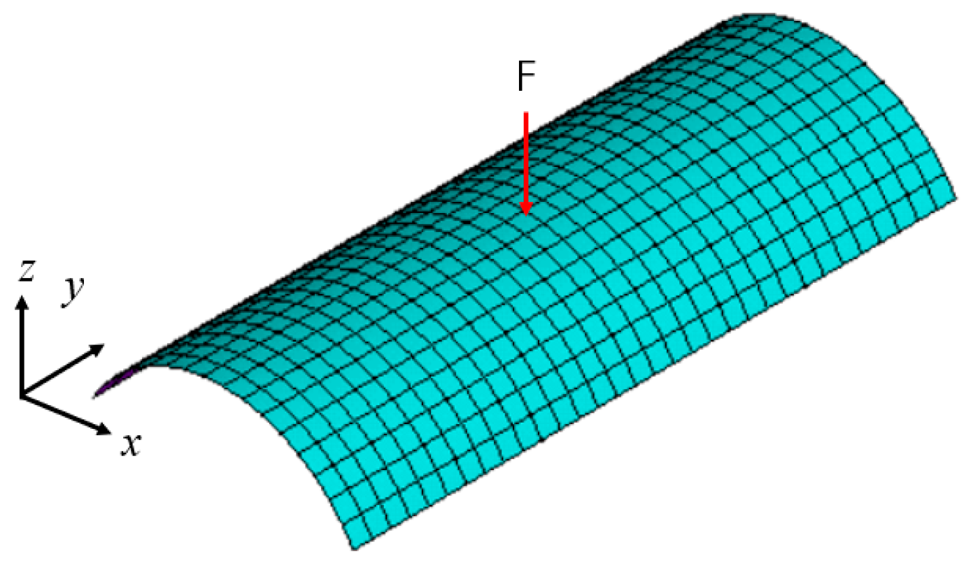
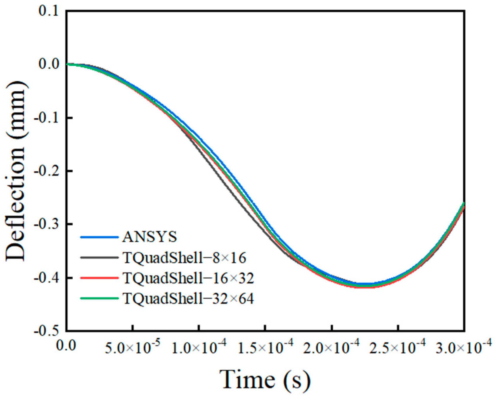
5.3. Cylindrical Shells Subjected to Impact Loads

The cylindrical shell depicted in Figure 6 possesses the following geometric dimensions: the length is $L=12 \mathrm{mm}$, the central angle is $\beta =120$°, the radius is $R=3 \mathrm{mm}$, the thickness is $a=0.125 \mathrm{mm}$, the elastic modulus of the material is $E={10}^7 \mathrm{MPa}$, the Poisson’s ratio is $u=0.3$, and the density is $\rho =2.5\times {10}^{-4} \mathrm{T}/{\mathrm{mm}}^3$. The busbar boundary is fixed, while the circumferential boundary is simply supported. Additionally, a concentrated impact load is applied at the central position, which linearly increases to $\mathrm{10,000} \mathrm{N}$ over $0\mathrm{s}~1.5\times {10}^{-4} \mathrm{s}$ and decreases to $0 \mathrm{N}$ over $1.5\times {10}^{-4} \mathrm{s}~3\times {10}^{-4} \mathrm{s}$.

Calculate the displacement of the center under the concentrated impact load using $8\times 16$, $16\times 32$, and $32\times 64$ TQuadShel1 elements, respectively. The results from the $16\times 32$ and $32\times 64$ TQuadShel1 elements align closely with those obtained from the $8\times 16$ Shell281 element in the ANSYS (2021) finite element software (Figure 7). The Shell281 element in ANSYS employs an eight-node quadrilateral element. When the mesh density of the TQuadShel1 element is four times that of the Shell281 element, the number of nodes in both elements becomes equal. To ensure calculation accuracy, the TQuadShel1 element utilizes a medium grid. The accuracy and reliability of the TQuadShel1 element calculations are satisfactory.

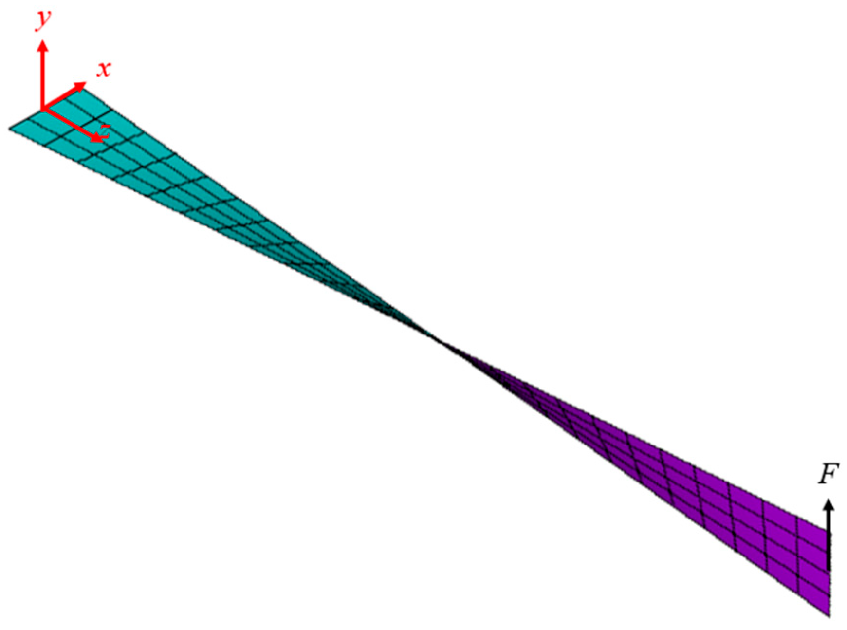
5.4. Twisted Cantilever Beam Subjected to Step Load

As shown in Figure 8, the twisted cantilever beam has a cross-sectional height of $\mathrm{H}=1.1 \mathrm{mm}$, a width of $\mathrm{W}=0.32 \mathrm{mm}$, and an axis length of $L=12 \mathrm{mm}$. The material properties include an elastic modulus of $E=2.9\times {10}^7 \mathrm{MPa}$, a Poisson’s ratio of $u=0.22$, and a density of $\rho =2.5\times {10}^{-4} {\mathrm{T}/\mathrm{mm}}^3$. The left end of the beam is anchored, while the centroid of the free end is subjected to a step load in the y-direction, which increases to $1.0 \mathrm{N}$ in $0\mathrm{s}~1\times {10}^{-2} \mathrm{s}$.

The $4\times 20$ TQuadShel1 element and $2\times 10$ Shell281 element of the ANSYS finite element software were utilized for the finite element analysis. Figure 9 illustrates the variation curve of the deflection at the free-end centroid of the twisted beam over time. The TQuadShel1 element achieves a maximum value of 1.1319 × 10⁻² mm at 4.0 × 10⁻³ s. The Shell281 element achieves a maximum value of 1.1320 × 10⁻² mm at 3.96 × 10⁻³ s. The maximum value obtained for the TQuadShel1 element is comparable to that of the Shell281 element, and the deflection-time curve demonstrates good agreement, indicating satisfactory calculation accuracy.

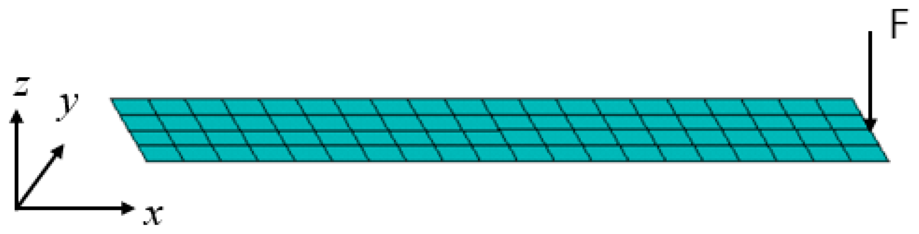
5.5. Rectangular Sheet Subjected to Impact Loads

The geometric dimensions of the matrix sheet shown in Figure 10 are as follows: length $L=1000 \mathrm{mm}$, width $W=100 \mathrm{mm}$, thickness $a=10 \mathrm{mm}$, elastic modulus $E=2\times {10}^5 \mathrm{MPa}$, Poisson’s ratio $u=0.3$, and density $\rho =7.8\times {10}^{-9}\mathrm{T}/{\mathrm{mm}}^3$. One short edge is fixed, while the midpoint of the opposite short edge is subjected to an impact load. This impact load increases linearly to $1200 \mathrm{N}$ in $0 \mathrm{s}~{10}^{-3} \mathrm{s}$ and decreases to $0 \mathrm{N}$ in ${10}^{-3} \mathrm{s}~2\times {10}^{-3} \mathrm{s}$.

As illustrated in Figure 11, to verify the calculation accuracy, the $2\times 10$ Shell281 element of ANSYS and the $4\times 20$ TQuadShell element were employed for finite element analysis to obtain the deflection-time curve of the vertex. During the application of the impact load, the thin plate exhibited a jumping–bending phenomenon. The displacement-time curve obtained through this method aligns well with the results from Shell281.

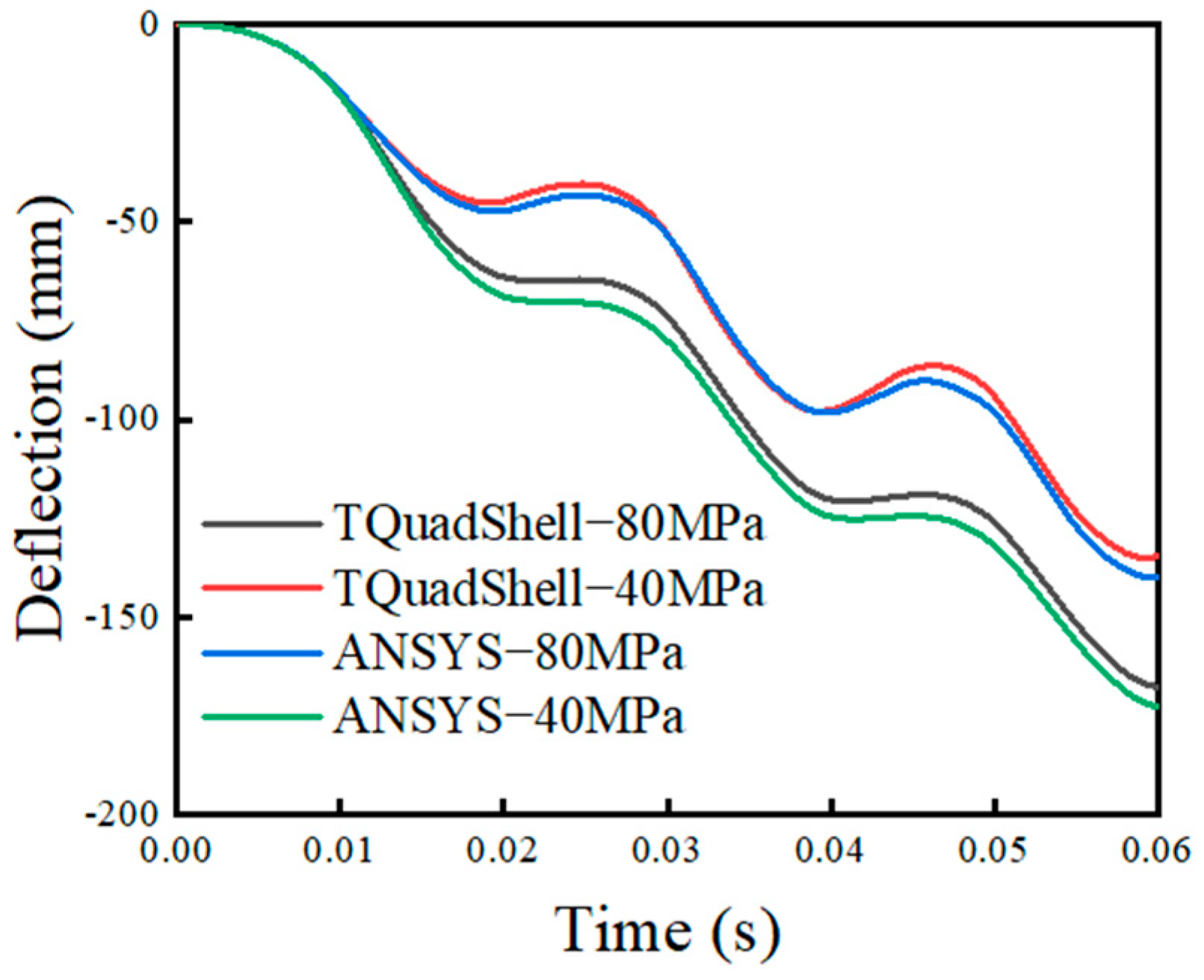
5.6. Ideal Elastic–Plastic Rectangular Sheet Subjected to Impact Loads

The calculation example mirrors that which is described in Section 5.5, but utilizes an ideal elastoplastic material. One short edge is fixed, while the midpoint of the opposite short edge is subjected to an impact load. The impact load increases linearly to −1200 N in $0\mathrm{s}~{10}^{-3}\mathrm{s}$, decreases linearly to 1200 N in ${10}^{-3}\mathrm{s}~2\times {10}^{-3}\mathrm{s}$, increases linearly to −1200 N in $2\times {10}^{-3}\mathrm{s}~3\times {10}^{-3}\mathrm{s}$, decreases linearly to 1200 N in $3\times {10}^{-3}\mathrm{s}~4\times {10}^{-3}\mathrm{s}$, and so forth, alternating between increases and decreases. The deflection-time curve was obtained under yield stresses of 40 MPa and 80 MPa, respectively.

As shown in Figure 12, both the elastic and plastic deformation of the thin plate occur during the application of the impact loads. When the rectangular thin plates are subjected to repeated loading and unloading under varying yield stress, the displacement-time curves produced with this method closely align with the results obtained from ANSYS using the Shell281 unit, indicating a high level of calculation accuracy.

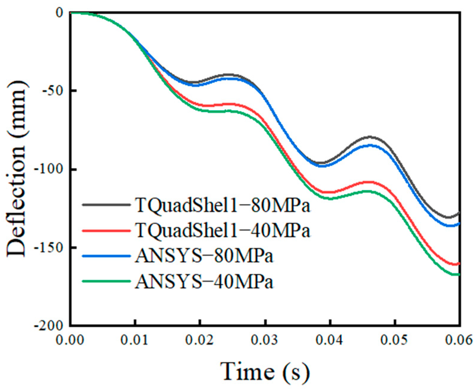
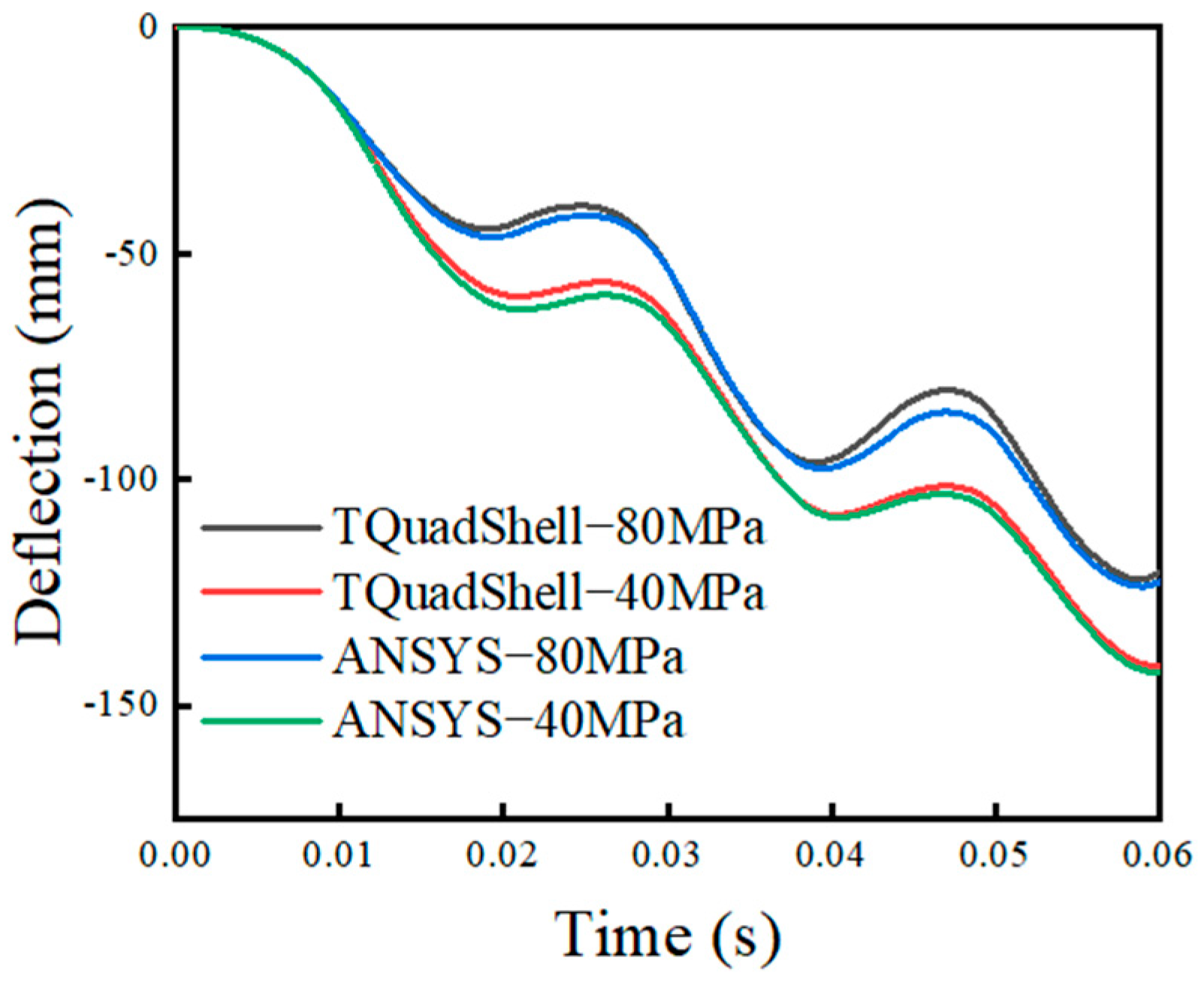
5.7. Isotropically Strengthened and Motion-Strengthened Elastoplastic Rectangular Thin Plates Subjected to Impact Loads

The calculation example is the same as that described in Section 5.6, but the isotropic linearly strengthened elastoplastic material and the kinetically linearly strengthened elastoplastic material are used, and the tangent modulus in both is $1.5\times {10}^4\mathrm{MPa}$. As illustrated in Figure 13 and Figure 14, the behavior of the isotropically strengthened and motion-strengthened elastic–plastic rectangular thin plates under an impact load aligns well with the results obtained from ANSYS using the Shell281 element. This demonstrates the high level of calculation accuracy and enhanced computational efficiency.

6. Conclusions

In this study, we enhance the four-node quadrilateral shell element to mitigate the effects of film self-locking, shear self-locking, and the zero-energy mode. The zero-energy mode is addressed by incorporating normal rotational degrees of freedom into the shell element and introducing additional stiffness through a penalty function. Shear self-locking is resolved using a mixed tensor interpolation strain method. Through analyses involving in-plane fragment inspection, curved fragment inspection, plane shells, curved shells, and twisted shells, we compare the results with those obtained from the ANSYS software. The findings demonstrate that the improved element effectively eliminates the influences of film self-locking, shear self-locking, and the zero-energy mode, resulting in satisfactory stability and calculation accuracy.

The calculation accuracy and stability of the four-node quadrilateral shell element, which is based on the neutral surface shell element, are comparable to those of the Shell281 element, which is based on the thin shell element in ANSYS. The introduction of rotational degrees of freedom around the z-axis enhances the membrane component of the four-node quadrilateral shell element, resulting in improved accuracy and adaptability. This study presents all the necessary formulas for code development, enabling comprehensive calculations of elastic–plastic problems and contributing to the advancement of independent finite element software.

This study has achieved significant progress in improving the computational accuracy of four-node quadrilateral shell elements, although there are still some limitations. Due to the singularity of the unit types and the difficulty of unit partitioning, computational analysis in complex structures displays areas for improvement. Future research will address these issues by developing three-node triangular shell elements. These works will aim to improve the comprehensiveness and reliability of shell units, ensuring their wider applicability and effectiveness in practical scenarios.

References

1. Dvorkin, E.N.; Bathe, K.J. A continuum mechanics based four-node shell element for general non-linear analysis. Eng. Comput. 1984, 1, 77–88. [Google Scholar] [CrossRef]
2. Wang, Z.; Sun, Q. Corotational nonlinear analyses of laminated shell structures using a 4-node quadrilateral flat shell element with drilling stiffness. Acta Mech. 2014, 30, 418–429. [Google Scholar] [CrossRef]
3. Ahmed, A.; Kapuria, S. A four-node facet shell element for laminated shells based on the third order zigzag theory. Compos. Struct. 2016, 158, 112–127. [Google Scholar] [CrossRef]
4. Versino, D.; Gherlone, M.; Di Sciuva, M. Four-node shell element for doubly curved multilayered composites based on the refined zigzag theory. Compos. Struct. 2014, 118, 392–402. [Google Scholar] [CrossRef]
5. Sussman, T.; Bathe, K.J. 3D-shell elements for structures in large strains. Comput. Struct. 2013, 122, 2–12. [Google Scholar] [CrossRef]
6. Kim, D.N.; Bathe, K.J. A triangular six-node shell element. Comput. Struct. 2009, 87, 1451–1460. [Google Scholar] [CrossRef]
7. Videla, J.; Natarajan, S.; Bordas, S.P.A. A new locking-free polygonal plate element for thin and thick plates based on Reissner-Mindlin plate theory and assumed shear strain fields. Comput. Struct. 2019, 220, 32–42. [Google Scholar] [CrossRef]
8. Bathe, K.J.; Lee, P.S.; Hiller, J.F. Towards improving the MITC9 shell element. Comput. Struct. 2003, 81, 477–489. [Google Scholar] [CrossRef]
9. Chapelle, D.; Bathe, K.J. Fundamental considerations for the finite element analysis of shell structures. Comput. Struct. 1998, 66, 19–36. [Google Scholar] [CrossRef]
10. Lee, P.S.; Bathe, K.J. On the asymptotic behavior of shell structures and the evaluation in finite element solutions. Comput. Struct. 2002, 80, 235–255. [Google Scholar] [CrossRef]
11. Bucalem, M.L.; Bathe, K.J. Higher-order MITC general shell elements. Int. J. Numer. Meth Eng. 1993, 36, 3729–3754. [Google Scholar] [CrossRef]
12. Bucalem, M.L.; Bathe, K.J. Finite element analysis of shell structures. Arch. Comput. Meth Eng. 1997, 4, 3–61. [Google Scholar] [CrossRef]
13. Belytschko, T.; Tsay, C.S. A stabilization procedure for the quadrilateral plate element with one-point quadrature. Int. J. Numer. Methods Eng. 1983, 19, 405–419. [Google Scholar] [CrossRef]
14. Koschnick, F.; Bischoff, M.; Camprubí, N.; Bletzinger, K.U. The discrete strain gap method and membrane locking. Comp. Meth Appl. Mech. Eng. 2005, 194, 2444–2463. [Google Scholar] [CrossRef]
15. Choi, C.K.; Paik, J.G. An efficient four node degenerated shell element based on the assumed covariant strain. Struct. Eng. Mech. 1994, 2, 17–34. [Google Scholar] [CrossRef]
16. Belytschko, T.; Leviathan, I. Projection schemes for one-point quadrature shell elements. Comput. Methods Appl. Mech. Eng. 1994, 115, 277–286. [Google Scholar] [CrossRef]
17. Allman, D.J. A Compatible Triangular Element Including Vertex Rotations For Plane Elasticity Analysis. Comput. Struct. 1984, 19, 1–4. [Google Scholar] [CrossRef]
18. Cook, R.D. On The Allman Triangle and a Related Quadilateral Element. Comput. Struct. 1986, 22, 1065–1067. [Google Scholar] [CrossRef]
19. Yunus, S.M. A Study of Different Hybrid Elements with and without Rotational DOF for Plane Stress/Plane Strain Problems. Comput. Struct. 1988, 30, 1127–1133. [Google Scholar] [CrossRef]
20. Huang, M.; Zhao, Z.; Shen, C. An effective planar triangular element with drilling rotation. Finite Elem. Anal. Des. 2010, 46, 1031–1036. [Google Scholar] [CrossRef]
21. MacNeal, R.H.; Harder, R.L. A refined four-noded membrane element with rotational degrees of freedom. Comput. Struct. 1988, 28, 75–84. [Google Scholar] [CrossRef]
22. Bathe, K.J.; Dvorkin, E.N. A formulation of general shell elements—The use of mixed interpolation of tensorial components. Int. J. Numer. Methods Eng. 1986, 22, 697–722. [Google Scholar] [CrossRef]
23. Bucalem, M.L.; Bathe, K.J. Locking behavior of isoparametric curved beam finite elements. Appl. Mech. Rev. 1995, 48, S25–S29. [Google Scholar] [CrossRef]
24. Ko, Y.; Lee, P.S.; Bathe, K.J. The MITC4+ shell element and its performance. Comput. Struct. 2016, 169, 57–68. [Google Scholar] [CrossRef]
25. Lee, P.S.; Bathe, K.J. The quadratic MITC plate and MITC shell elements in plate bending. Adv. Eng. Softw. 2010, 41, 712–728. [Google Scholar] [CrossRef]
26. Abedian, A.; Parvizian, J.; Düster, A.; Rank, E. The finite cell method for the J2 flow theory of plasticity. Finite Elem. Anal. Des. 2013, 69, 37–47. [Google Scholar] [CrossRef]
27. Szabó, L. A semi-analytical integration method for J2 flow theory of plasticity with linear isotropic hardening. Comput. Methods Appl. Mech. Eng. 2009, 198, 2151–2166. [Google Scholar] [CrossRef]
28. Martínez-Pañeda, E.; Fleck, N.A. Mode I crack tip fields: Strain gradient plasticity theory versus J2 flow theory. Eur. J. Mech.-A/Solids 2019, 75, 381–388. [Google Scholar] [CrossRef]
29. de Borst, R. A generalisation of J2-flow theory for polar continua. Comput. Methods Appl. Mech. Eng. 1993, 103, 347–362. [Google Scholar] [CrossRef]
30. Mousavi, F.; Jafarzadeh, S.; Bobaru, F. An ordinary state-based peridynamic elastoplastic 2D model consistent with J2 plasticity. Int. J. Solids Struct. 2021, 229, 111146. [Google Scholar] [CrossRef]
31. Yu, B.; Yin, X.; Jiang, L.; Xiao, X.; Wang, C.; Yuan, H.; Chen, X.; Xie, W.; Wang, H.; Ding, H. Analysis of plastic yield behavior during impact of a rigid sphere on an elastic-perfectly plastic half-space. Int. J. Mech. Sci. 2023, 237, 107774. [Google Scholar] [CrossRef]
32. Iandiorio, C.; Salvini, P. Elastic-plastic analysis with pre-integrated beam finite element based on state diagrams: Elastic-perfectly plastic flow. Eur. J. Mech.-A/Solids 2023, 97, 104837. [Google Scholar] [CrossRef]
33. Lou, Y.; Zhang, C.; Wu, P.; Yoon, J.W. New geometry-inspired numerical convex analysis method for yield functions under isotropic and anisotropic hardenings. Int. J. Solids Struct. 2024, 286, 112582. [Google Scholar] [CrossRef]
34. Roubaud, F.; Morin, L.; Remmal, A.; Marie, S.; Leblond, J.B. A Gurson-type layer model for ductile porous solids containing ellipsoidal voids with isotropic and kinematic hardening. Eur. J. Mech. -A/Solids 2024, 104, 105114. [Google Scholar] [CrossRef]
35. Mehani, N.; Roy, S.C. Modified isotropic and kinematic hardening equations for 304L SS under low cycle fatigue. Comput. Mater. Sci. 2024, 240, 112999. [Google Scholar] [CrossRef]
36. Krabbenhøft, K.; Krabbenhøft, J. Simplified kinematic hardening plasticity framework for constitutive modelling of soils. Comput. Geotech. 2021, 138, 104146. [Google Scholar] [CrossRef]
37. Yu, H.Y.; Chen, S.J. A mixed hardening model combined with the transformation-induced plasticity effect. J. Manuf. Process. 2017, 28, 390–398. [Google Scholar] [CrossRef]
38. Lei, P.; Meng, S.; Wu, J.; Liu, Z.; Imtiaz, H.; Feng, H.; Zhou, J.; Liu, B. Is the Jaumann Stress Rate Applicable?—Discussions on Choosing Proper Rate Expressions of a Finite Deformation Constitutive Model. Int. J. Appl. Mech. 2023, 15, 2350097. [Google Scholar] [CrossRef]
39. Belytschko, T.; Lin, J.I.; Chen-Shyh, T. Explicit algorithms for the nonlinear dynamics of shells. Comput. Methods Appl. Mech. Eng. 1984, 42, 225–251. [Google Scholar] [CrossRef]
40. Belytschko, T.; Leviathan, I. Physical stabilization of the 4-node shell element with one point quadrature. Comp. Meth App Mech. Eng. 1994, 113, 321–350. [Google Scholar] [CrossRef]
Figure 1. The DOF of a three-node straight line.
Applsci 14 09186 g001
Figure 2. Four-node quadrilateral shell element coordinate system.
Applsci 14 09186 g002
Figure 3. Distribution map of shear strain rate interpolation correlation points.
Applsci 14 09186 g003
Figure 4. Plastic analysis flowchart.
Applsci 14 09186 g004
Figure 5. Patch test mesh.
Applsci 14 09186 g005
Figure 6. Cylindrical shell.
Applsci 14 09186 g006
Figure 7. Curve of deflection at the center of the cylindrical shell over time.
Applsci 14 09186 g007
Figure 8. Twisted cantilever beam.
Applsci 14 09186 g008
Figure 9. The variation curve of the y-axis deflection with time at the free-end centroid.
Applsci 14 09186 g009
Figure 10. Rectangular thin plate.
Applsci 14 09186 g010
Figure 11. The deflection (z-displacement) curve with the impact load.
Applsci 14 09186 g011
Figure 12. Time variation curve of deflection of ideal elastoplastic material under impact load.
Applsci 14 09186 g012
Figure 13. Time variation curve of deflection of isotropically strengthened material under impact load.
Applsci 14 09186 g013
Figure 14. Time variation curve of deflection of motion-strengthened material under impact load.
Applsci 14 09186 g014