Abstract
We aimed to investigate the fluid–solid–ice coupling mechanism as structures break through ice into water. Using LS–DYNA finite element software, a numerical simulation method is established, based on the ALE flow–solid coupling method, and the penalty function contact algorithm, which describes the structure–ice–water coupling interaction. The Eulerian algorithm is used to describe the air and water domains, while the Lagrange method is applied to the wedge and ice structure. The mechanical properties of ice are characterized using the elastic–plastic failure strain model. The feasibility of simulating the entry of structures into water via the ALE method is demonstrated by comparing the experimental and simulation results of wedges entering into water. The applicability of the ice material model in simulating collision–induced breakup is verified by comparing a simulation of a rigid plate hitting a spherical head of ice, with results from the ISO standard. The effects of water during icebreaking are assessed by simulating a wedge breaking through ice into water, as well as through ice without water. Additionally, the ice breakup and motion response of the wedge under different working conditions are compared by varying the wedge mass and icebreaking speed.
1. Introduction
Launching lifeboats and landing airplanes on the sea surface in ice-covered areas are affected by the presence of ice on the water. However, current research mainly focuses on theoretical and experimental methods. Due to differences in water-based testing, the structure of an icebreaking object in water should consider the structure–ice–water interaction. However, the costs of testing are higher and the conditions are more demanding. As a result, after years of development, numerical simulation methods have become increasingly favored by scholars. In recent years, these methods have matured significantly, including traditional computational fluid dynamics (CFD), near-field dynamics (PD), the finite element method (FEM), the smoothed particle hydrodynamics (SPH) method, and the discrete element method (DEM). Numerical simulations can be used to construct a structure–ice–water mixing model and simulate the physical phenomenon of icebreaking. Scholars from various countries have begun adopting numerical simulations for structural, waterborne icebreaking.
Aniket Patil et al. [1] used the SPH method, simulating each piece of broken ice as a combination of particles. Through a pulling test experiment, they investigated the mechanical and physical properties of ice in a broken ice region by changing the parameters, such as the void fraction, cohesion, and friction angle, providing a preliminary method to understand the icebreaking process. Zhang et al. [2] validated the smoothed particle hydrodynamics (SPH) approach using the Drucker–Prager plasticity model, combined with a 1:20 scaling ratio hull model, to simulate impacts with level ice for validation purposes. An inter-comparison of the results confirmed the applicability and reliability of the SPH approach for simulating structure–ice–water scenarios, as well as the Drucker–Prager model for simulating the icebreaking process. Liu et al. [3] simulated the process of continuous icebreaking using the combined smoothed particle method (CSPM), integrated with a density-corrected and artificial stress-corrected low-speed collision model. They investigated the icebreaking resistance and immersion resistance of the hull during icebreaking.
The ice damage process is a discontinuous and complex material breakage involving the structure–ice–water interaction, and near–field dynamics is a meshless approach to solving the equations of motion in integral form, with clear advantages for simulating damage in complex materials. Liu et al. [4] employed a non–local, meshless “near–field dynamics” numerical method, based on the integral form, to simulate interactions between horizontal ice and cylindrical, vertical, and rigid structures, at different velocities. They also investigated the relationship between the damage length of the icebreaking region and ice thickness, concluding that the damage length is 0.150.2 times the ice thickness. Sandro et al. [5] proposed a numerical method to simulate local ice loads generated by ship–ice interactions with horizontal ice and calculated the resulting icebreaking resistance components. Ren et al. [6] developed a structure–ice–water numerical model using a combination of PD, BDIM, and VOF to simulate icebreaking and water ingress for a rigid sphere. They also analyzed the crack extension paths of the ice cap, the shape of the cavity, the pressure and velocity fields, and the motion of the sphere during icebreaking and water ingress, concluding that the ice loads on the sphere were much larger than the water loads.
From simulating ice to calculating the resistance of icebreaking, the aforementioned research and analysis have made significant contributions. For research on icebreaking, it is more important to conduct simulations or experimental analyses of icebreaking processes.
Wu et al. [7] investigated the dynamic response and energy absorption characteristics of aluminum honeycomb sandwich panels (AHSPs) under wedge-shaped ice impact. Using the concrete intrinsic ice model, they established a finite element model of the AHSPs under ice impact. The ice impact experiments validated the accuracy and reliability of the numerical model. They discussed the effects of impact failure and energy dissipation of the ice impactor on the dynamic mechanical behavior of AHSPs. P. Bateman et al. [8] developed a technique to simulate the fracture mechanics of ice under bending, compressive, and tensile loading, based on a DEM approach. Jang et al. [9,10] used a 3D DEM with parallel bonds to simulate realistic ice breakup, which was combined with an in–house hull–mooring coupled dynamic analysis program, CHARM3D, to explore the interaction of level ice with floating offshore structures such as moorings. They further extended the DEM coupling methodology to address the surge in floating structures under level ice loading in the time domain. Ji et al. [11] used CUDA C++ to establish a DEM-FEM coupling method to simulate the interaction between sea ice and offshore wind turbines. The method considered not only the effects of individual factors in the breaking process, but also the effects of the mechanical properties and structural motions of sea ice on distribution. Marnix et al. [12] developed an ice tank test model based on the DEM and explored the repeatability of the ice tube icebreaking test by adjusting the initial position of the ice floe. Zhu et al. [13] established an ice–mooring numerical model based on the DEM. Considering factors, such as ice load, mooring force, hydrodynamics, and other factors, they simulated the interaction between a semi–submersible structure and level ice and analyzed the effect of ice thickness on ice load. Long et al. [14,15] used a GPU–based DEM to analyze the fracture length of the ice cap and ice load on a narrow conical structure. The numerical model was validated with the measured data from the Bohai Sea and the HSVA model test. They used the DEM results to discuss the effects of ice thickness, ice speed, and cone diameter on the icebreaking length and ice load on the narrow cone structure. Jeong et al. [16] examined variables affecting the ship’s resistance—channel width, ice break–up size, ice concentration and ice thickness—and used acausal regression analysis to derive the relationship between the four variables. Based on this, they established a prediction equation for the resistance to ice buildup. Liu et al. [17] simulated the interaction between the ship hull and horizontal ice using SDEM and DPDEM, comparing the sphere–based DEM (SDEM) and expansion–polyhedron–based DEM (DPDEM) to determine the ice resistance on the ship hull. This was used to analyze the ship–ice interaction. Jou et al. [18] modeled the buildup of bonded spherical particles in the ice continuum using the DEM, which may break due to ship–ice interactions, and studied the failure modes. They used discrete spherical elements to model the ice cap and studied the ice loads. In addition, the finite element method with beam elements was used to model the ice vortex excitation of the conduit rack platform, and an effective transport scheme between the bond–breaking spherical elements and beam elements was proposed.
In 2019, Marnix et al. [19] verified the applicability of CFD + DEM modeling for studying ships with broken ice. Building on this, Huang et al. [20] developed a CFD+ DEM model to simulate ship–broken ice interactions, improving the DEM aspect by modeling each ice floe with multiple DEM elements to investigate how the ship’s advancing speed affects the distribution and motion of the ice around the ship. He et al. [21] developed a fragile ice cap model by stacking a single layer of granular DEM particles. Based on this, the first numerical model based on a coupled CFD–DEM was developed to simulate the ice cap breakup under the action of regular incident waves. Tang et al. [22] investigated the ship–ice–water interaction of the KRISO container ship (KCS) model in icy area using CFD–DEM simulations with the commercial STAR–CCM+ software version 2310. Jeon et al. [23] simulated the material behavior of ice and the fracture behavior of structural collisions using a self–developed finite element analysis program based on damage mechanics and the elemental erosion technique combined with the Drucker–Prager model in the commercial finite element program ABAQUS. They obtained the ice resistance acting on rigid structures at several different forward speeds. Pernas–Sánchez et al. [24] developed an ontological relationship for ice at high strain rates, implementing its numerical integration algorithm, using three different methods (SPH, ALE, and Lagrangian) in the commercial LS-DYNA R11.0 software. Xu et al. [25] studied the fracture mechanism of horizontal ice by simulating a collision between ice and a rigid hull structure, using an extended finite element approach. They used a transversely isotropic material model and a bonded zone model to simulate the overall response of horizontal ice.
From the above analysis, it is evident that most current research focuses on characterizing the mechanical behavior of ice and investigating ice loads. Relatively few studies address the structure–ice–water–air coupling collision, especially the icebreaking of structures into water. To address the future scenario of launching lifeboats on the sea surface in icy regions, this study takes a wedge as the research object, and uses LS-DYNA R11.0 software and the ALE fluid–structure coupling method to establish a numerical model of the wedge–ice–water–air coupled collision, simulating the process of a wedge breaking through ice into water. The first section of this paper summarizes the ALE method and the penalty function calculation method. The second part of this study verifies the applicability of the ALE method in simulating water ingress by performing wedge water ingress tests and comparing test data. The applicability of LS-DYNA R11.0 in simulating the ice–structure collision response is further validated by comparing P–A theory results with numerical simulations of a rigid plate colliding with a spherical body. The results, presented in Section VI, demonstrate the effects of different impact velocities and wedge masses on the wedge breaking through ice into water.
2. Analysis Method for Wedge–Ice–Water–Air Coupled Collision
2.1. The Introduction of Arbitrary Lagrangian–Eulerian (ALE) Algorithm
The arbitrary Lagrangian–Eulerian (ALE) algorithm is often used in the numerical simulation of fluid–structure coupling. This method combines the characteristics of the Lagrange method and the Euler method: the Lagrange method is used to track the motion at the boundary of the material structure, while the Euler method is employed to handle the internal mesh elements, thus avoiding severe distortion of the mesh. It has overlapping characteristics with the geometry and mesh of structures and fluids, which can reduce the calculation scale. The ALE algorithm uses the Euler mesh in the flow field and the Lagrange mesh in the structure. The two meshes exchange information through a penalty function algorithm at the fluid–structure coupling interface to realize the transfer of flow field and structure variables. Figure 1 shows the difference between the Lagrange method, Euler method, and the ALE method.
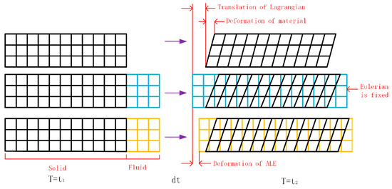
Figure 1.
Differences between the Lagrange, Euler and ALE algorithms.
2.2. Governing Equations
The ALE algorithm is used to solve the velocity and displacement of the flow field grid using conservation equations. In addition to the Lagrange and Euler coordinates, a reference coordinate system is introduced into the ALE algorithm to describe the flow field governing equation. If the velocity of the material is v and the velocity of the mesh is u, then the relative velocity w = v − u, where u = v in the Lagrange form and u = 0 in the Eulerian form. When the mesh velocity is longer, the governing equation of the fluid in the ALE algorithm is transformed into the governing equation of the fluid in the Euler algorithm. Therefore, in the ALE algorithm, the expressions of mass conservation, momentum conservation, and energy conservation can be obtained, respectively, as follows:
where denotes time; is density; is the particle displacement; is force; is the energy; and is tensor of stress.
2.3. Penalized Function Coupling Approach
The coupling between the fluid and the structure is handled using the penalty function coupling method [26,27,28]. The principle of the penalty function calculation is similar to a spring system (as shown in Figure 2). This coupling method calculates the pressure at each point on the contact surface through the relative displacements and the time derivatives. Then, the pressure is applied to the nodes of the contact surface to prevent the fluid from infiltrating into the structure. The coupling force is denoted as follows:
where denotes the stiffness coefficient of the penalty function; denotes the penetration depth; and force acts on both the slave and master structures in opposite directions to ensure the balance of forces on the contact surfaces. denotes the fluid force at the fluid node, and denotes the force at the structural coupling node.
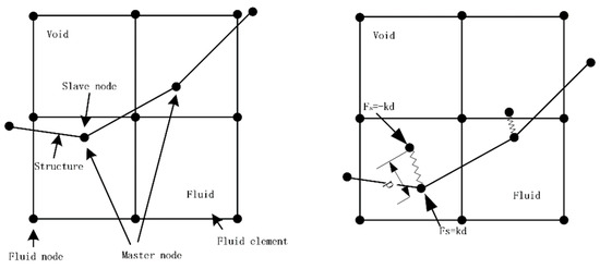
Figure 2.
Diagram of the penalty function coupling algorithm.
The setting of the stiffness coefficient of the penalty function is challenging when performing simulations. When the stiffness coefficient k of the penalty function reaches infinity, the penetration depth decreases to zero. Although the contact surface will not be penetrated, it will affect the overall stiffness. The stiffness coefficient of the penalty function is expressed by the following equation:
where is the scaling factor for the stiffness of the penalty function; denotes the bulk modulus of the fluid; is the volume of the fluid cell that contains the master material node; and is the average area of the structural elements associated with the slave nodes on the coupling surface.
By choosing the appropriate value of , the interpenetration between the master and slave materials can be effectively controlled, while the overall stiffness of the system will be significantly affected.
3. The Numerical Model of Wedge–Ice–Water–Air Coupled Collision
3.1. Description of Problem
The process of a wedge falling from a high altitude, breaking through ice into water involves interactions between the wedge, the ice, the air, and the water. Among these, the wedge and ice are described using the Lagrange algorithm, while the air and water are described using the Euler algorithm. The wedge is 0.4 m in length, 0.2 m in width, 0.1 m in height, 0.05 m in thickness, and the slope rise angle is 60°. The ice has a thickness of 0.01 m, a length of 0.4 m, and a width of 0.3 m. The water domain has a size of 0.8 m × 0.4 m × 0.4 m, while the air domain has a size of 0.8 m × 0.4 m × 0.1 m. The mesh size for both the air and water domains is 0.008 m. The geometric dimensions of the model are shown in the Figure 3.
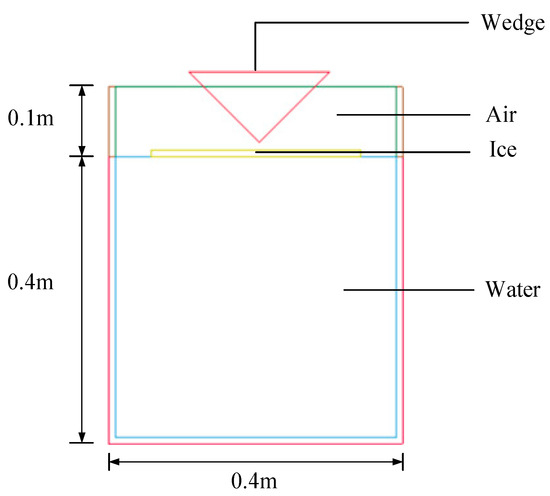
Figure 3.
Simulation of wedge breaking ice into water.
3.2. Material Model and Equation of State
The process of the wedge breaking through ice into water involves four materials: wedge, ice, air, and water. The wedge and the ice material model will be introduced in the following sections. For air and water, it is necessary to define the material model and the corresponding fluid state equation to solve the governing equation.
In LS–DYNA, the material properties of air and water can be simulated using the empty material (*MAT_NULL) model, by simply specifying the fluid density. The equation of state for the fluid describes the relationship between volume deformation and pressure. In this study, the linear POLYNOMIAL equation of state is used for air, and the GRUNEISEN equation of state is used for water.
The state equation for air medium in LS–DYNA is defined by the keyword *EOS–LINER–POLYNOMIAL. In the linear POLYNOMIAL equation of state, the relationship between pressure value and relative volume is expressed as follows:
where – are the constant; is the relative volume; and is the specific internal energy of the fluid.
In this study, the values of each constant are , , and .
The state equation of water is defined by the keyword *EOS–GRUNEISEN in the LS–DYNA program. The GRUNEISEN equation of state results in different expressions between pressure and relative volume depending on the compression or expansion state of the material. The pressure expression in the compressed state is as follows:
where is the fluid density; is the speed of sound in water; is the specific internal energy of the fluid; and , , , , and are the input parameters related to pressure propagation. The constants for the water materials used in this study are shown in Table 1.

Table 1.
Water parameters.
In this study, the wedge is defined as a rigid body, and the elastic–plastic strain rate material model is selected for the ice layer. The interaction between the wedge and the ice layer, as well as the interaction between the ice cells, is realized using the erosion contact algorithm, where the ice cells are constantly damaged and cracks are formed by removing the failing cells. Once the grid cells fail and the contact surfaces are changed, the surface shapes can be re–established via erosion contact.
4. Validation of Numerical Methods
4.1. Validation of the Simulation of the Ice Constitutive Model
The selected ice constitutive model is the 13th material model *MAT_ISTROPIC_ ELASTIC_FAILURE [29] from the LS–DYNA material library. When the effective plastic strain reaches the failure strain or the pressure reaches the failure criterion, the unit loses the ability to carry the stress, and the bias stress is set to zero. This means the material is realized as a fluid state.
To verify the accuracy of the ice principal model, this study numerically simulates the rigid plate impacting spherical head ice and compares it with the P–A theory curve proposed by Masterson in 2009 [30]. The model is shown in Figure 4.
where P is the pressure (MPa) and A is the contact area between the rigid plate and the ice (m2).
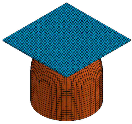
Figure 4.
The rigid plate hits the ball head ice.
Spherical ice is modeled using solid units. The model consists of a solid hemisphere with a radius of 1 m and a solid cylinder; the height of the solid cylinder is 1 m. The material parameters of the sea ice are shown in Table 2. The rigid plate is modeled as a solid with a side length of 2.5 m; the material parameters are shown in Table 3. The rigid plate is given a constant downward initial velocity v = 2 m/s to hit the spherical head ice.
Table 2.
Material parameters of ice.
Table 3.
Material parameters of rigid plate.
Contact is made between the spherical head ice and the rigid plate using the erosion contact keyword *CONTACT_ERODING_SURFACE_TO_SURFACE in the LS–DYNA software. This software can be used to automatically delete the failed unit and automatically search for the effective unit to establish contact when the plastic strain of the ice unit reaches the failure strain or the pressure reaches the failure truncation pressure.
Figure 5 shows a comparison of the P–A curves obtained from the rigid plate–bulb ice in this study with the ISO standard curves. As seen, the results fit well, thus verifying the reliability of the principal ice model material used in the collision simulation.
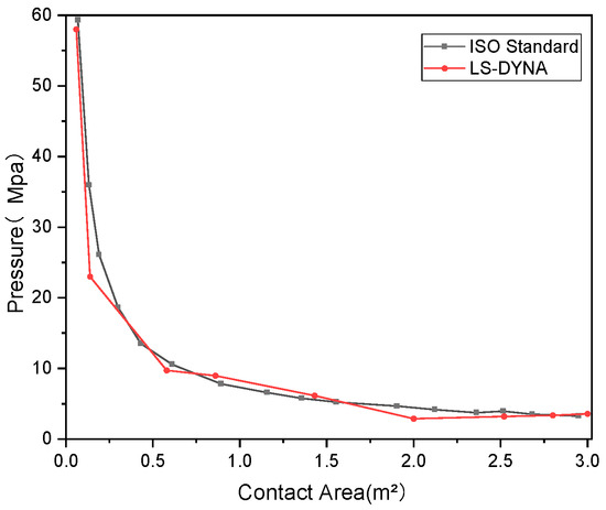
Figure 5.
Spherical simulation of rigid plate impact and variation in ISO theoretical ice pressure with area.
It should be noted that, considering the changes in material parameters caused by the size of the ice, these parameters can be modified in the software when conducting different simulations.
4.2. Verification of the Wedge Breaking into Water
To verify the accuracy and feasibility of the ALE method used to analyze fluid–structure coupling problems, a simulation and test of the wedge breaking into the water are carried out using this method. Then, the simulation results are compared with the test results.
Taking the hollow wedge made of Q235 steel as the research object, a test of the vertical water entry of the wedge is carried out using self–developed test tooling. The test model is shown in Figure 6. Its dimensions are 0.4 m in length, 0.2 m in width, 0.1 m in height, and 0.05 m in thickness; the angle of inclination is 60° and the data acquisition system is DH5925N. The test tooling mainly consists of a bracket and electromagnet. A high–speed video camera is used to observe the details of the wedge entering the water, and acceleration sensors are symmetrically placed in two locations to test whether the wedge enters the water vertically and from a height of 0.2 m.

Figure 6.
Wedge test model.
For the vertical water entry test, it is necessary to ensure that the wedge remains vertical as it enters the water. Symmetrically distributed acceleration sensors are used to estimate verticality due to the uniform mass distribution of the wedge. In addition, since the water surface is static, when both acceleration sensors register similar data, it indicates that the wedge is perpendicular to the water surface upon entry.
As seen in Figure 7, when the wedge enters the water, both the time of peak acceleration arrival and the size of peak acceleration are the same on both sides. In addition, observations from the high–speed camera show no deflection, confirming that the wedge enters the water vertically.

Figure 7.
Wedge acceleration test values.
For the numerical simulation, the wedge model used is identical to the one used in the test, and the material is treated as a rigid body, though the fluid domain is appropriately reduced. The size of the water domain is 0.8 m × 0.4 m × 0.4 m, while the size of the air domain is 0.8 m × 0.4 m × 0.1 m. The mesh size is 1 mm and hexagonal, and the material is defined using *MAT_NULL. The simulation model diagram is shown in Figure 8.
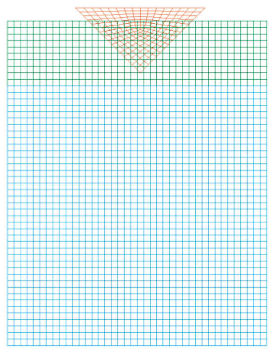
Figure 8.
Simulation model diagram of wedge entering the water.
The fluid domain is modeled using the Eulerian algorithm, while the wedge is modeled by the Lagrangian algorithm. The keywords *LINER–POLYNOMIAL and *EOS–GRUNEISEN are used to realize the equations of state of the air and water, respectively. Their parameters are shown in Section 3.2. Non–reflective boundaries are adopted to prevent the wall surface from affecting the simulation results of the wedge entering the water.
The test results are shown in Figure 9. The peak magnitude of the wedge’s inflow acceleration, the overall trend of the curve, and the inflow time are consistent with the test values, which proves the feasibility of the ALE method in dealing with the wedge inflow problem.
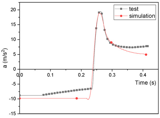
Figure 9.
Testing for wedge entering water and simulation acceleration results.
5. Wedges Vertically Breaking through Ice into Water
5.1. Verification of Mesh Convergence
Before conducting the formal numerical computation, it is necessary to perform a mesh convergence validation analysis to avoid the influence of mesh quality on the computational accuracy and efficiency. This step also ensures that the number of meshes does not affect computational accuracy while selecting the mesh that offers the highest computational efficiency.
In this study, considering the feasibility of computing resources and mesh size, 10, 8, and 4 mm hexahedral meshes are selected for mesh convergence analysis. The results are shown in Figure 10. The trends of the three curves and the peak results are similar. However, the 10 mm mesh shows a larger value at the secondary peak, while the 8 and 4 mm curves fit better. Considering the computational efficiency, the 8 mm mesh cell is selected for the computation.

Figure 10.
Acceleration graphs of different meshes.
5.2. Simulation Setting
The numerical model of a wedge vertically breaking through ice into water consists of four parts: wedge, ice, water, and air domains. The model is first designed, and, then, the simulation is carried out using the ALE method. The wedge parameters and dimensions are the same as mentioned above but with a solid wedge and a vertical fall speed of 10 m/s. The initial speed is defined using the keyword *INITIAL_VELOCITY_NODE. In addition, non–reflective boundary settings are used on the outer side of the fluid domain to avoid the influence of boundary effects. The coupling between the geometric model and the fluid domain is set using the keyword *CONSTRAINED_LAGRANGE_IN_SOLID.
The material parameters of ice are the same as mentioned above, and the dimensions are set to 0.4 m × 0.3 m × 0.02 m. The hydrostatic pressure is initialized using *INITIAL_HYDROSTATIC_ALE, while the fluid–solid coupling between the ice, wedge, and fluid regions is realized using *CONSTRAINED_LAGRANGE_IN_SOLID, and *CONTACT_ERODING_SURFACE_TO_SURFACE is used to model erosion contact between the ice sheet and wedge. Then, the simulation calculation is performed, and the post–processing data associated with the simulation are exported using *DATABASE_ABSTAT.
5.3. Forms of Ice Damage
As shown in Figure 11a,b, the breakup of the ice sheet mainly occurs when the wedge impacts the ice surface, during the stage above the water surface.
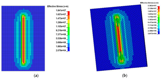
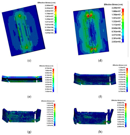
Figure 11.
Ice stress map with water environment. (a) T = 3.5845 ms. (b) T = 3.799 ms. (c) T = 4.3922 ms. (d) T = 4.9848 ms. (e) T = 5.8396 ms. (f) T = 7.1993 ms. (g) T = 11.82 ms. (h) T = 18.38 ms.
The ice sheet destruction slows down after the wedge is submerged in the water. When the wedge first contacts the ice, the lower surface of the ice layer experiences tensile strength, which sharply increases to 18 MPa, followed by tensile damage along the length of the wedge from the furthest point. The stress increases further to 25 MPa, and symmetrically distributed cracks begin to appear on the upper surface of the ice layer, as shown in Figure 11c. As the wedge continues to descend, longitudinal cracks on the lower surface of the ice layer gradually extend along the length, forming penetrating cracks through these longitudinal fissures, as shown in Figure 11d.
Simultaneously, transverse cracks gradually start to appear on the lower surface of the ice layer at both ends of the wedge tip. Over time, these cracks spread to both the upper and lower surfaces of the ice layer. As the ice layer enters the water, the maximum stress begins to gradually reduce. Additionally, as the contact area of the wedge and the ice layer increases, the stress initially concentrates at the wedge tip and spreads throughout the ice. The area of ice damage increases, but the rate of damage decreases.
After the ice layer enters the water, under the extrusion of both the wedge and the water, the two ends of the ice layer begin to bend inward toward the center. This leads to the impact of the ice layer on the surface of the wedge, resulting in the second stress peak. Subsequently, the ice layer starts to break down more rapidly. Within a calculation time of 0.02 s, the entire ice layer becomes seriously damaged. The two ends of the ice layer fracture; however, the part in contact with the wedge’s supper surface remains intact due to compression.
To further investigate the effect of water on the icebreaking process of the wedge, a wedge–ice sheet model in a fluid–free domain is established. As shown in Figure 12, the pre–destruction of the ice layer is more rapid in the absence of water, and the ice layer is not damaged in the presence of water at t = 3.588 ms, while the lower surface of the ice layer is damaged in the absence of water. This shows that the presence of water slows the rate of ice destruction.
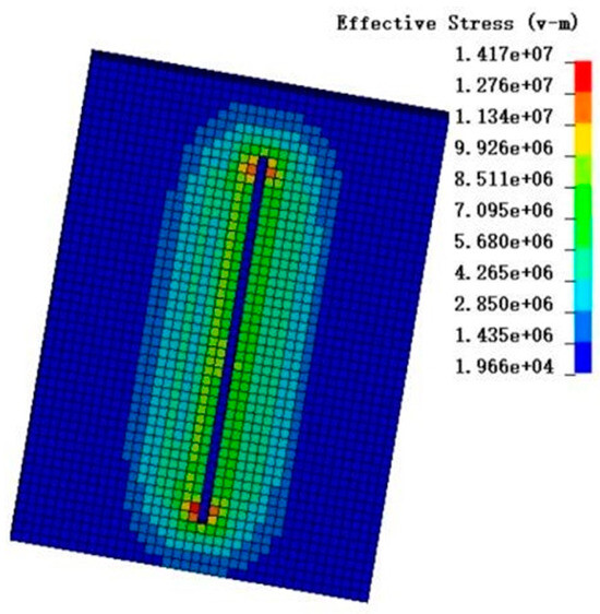
Figure 12.
Ice stress map of anhydrous environment. T = 3.588 ms.
6. Factors Affecting the Result of the Wedge Breaking through Ice into Water
6.1. Wedges with Different Icebreaking Speeds
To investigate the effect of different water impact speeds on the wedge breaking through ice into the water, this study simulates different water impact speeds (V = 10, 20, and 30 m/s) while keeping the wedge mass constant (m = 23.55 kg). Figure 13 shows the damage to the ice surface at different speeds at t = 0.02 s. From left to right, the initial speed of the wedge is V = 10, 20, and 30 m/s.
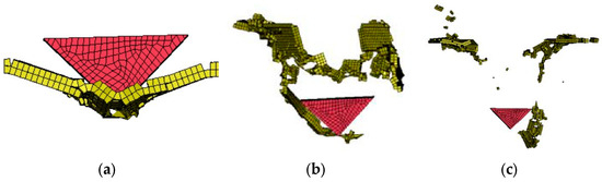
Figure 13.
Ice destruction at different speeds. (a) V = 10 m/s. (b) V = 20 m/s. (c) V = 30 m/s.
The results show that the faster the speed, the greater the damage to the ice layer. When the speed of the wedge is V = 10 m/s, the ice layer is not completely destroyed. When the speed is 20 m/s, a large area of the ice layer is destroyed, with some sections failing and disappearing. When V = 30 m/s, most of the ice layer disappears, as it has been almost entirely broken. Figure 14 shows the trend of acceleration at different speeds.
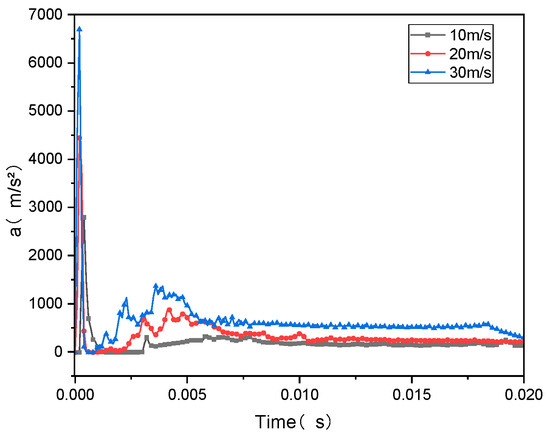
Figure 14.
Collision acceleration at different speeds.
The results in Figure 15 demonstrate that the larger the impact velocity, the greater the acceleration of the wedge during collision, and the more pronounced the velocity lag during the impact phase.

Figure 15.
V/Vx at different crash speeds.
6.2. Different Wedge Masses
This study also investigates the effect of different wedge masses on icebreaking by simulating wedges of different masses at a constant entry velocity (V = 10 m/s). Figure 16 shows the damage to the ice surface at different masses at t = 0.02 s. From left to right, the mass of the wedge is m = 23.55, 33.55, and 43.55 kg. The results show that the quality of the wedge has a small effect on the extent the ice layer damage, with no significant differences in the impacts of the three masses.
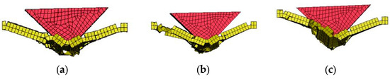
Figure 16.
Ice damage at different masses. (a) m = 23.55 kg. (b) m = 33.55 kg. (c) m = 43.55 kg.
Figure 17 shows the acceleration results as the wedge breaks through ice into water. It is evident that, during this process, the load from the ice is much larger than from the water. Upon contact with the ice surface, the wedge experiences a larger impact, causing the acceleration to peak and the speed to decay rapidly.
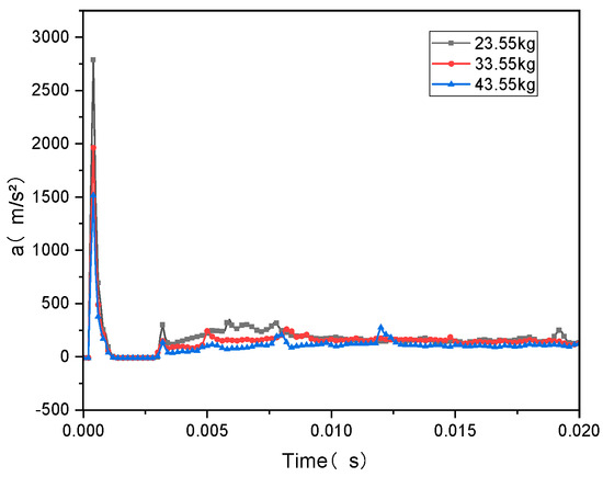
Figure 17.
Collision acceleration at different masses.
As shown in Figure 18, the slope of V/Vx is initially steep, but the rate of speed begins to gradually decrease as the acceleration begins to decrease after reaching its peak. During the collision with the ice layer and the subsequent breakthrough into the water, the effect of the wedge’s mass on peak acceleration is very clear. When the wedge mass is 23.55 kg, 33.55 kg, and 43.55 kg, the acceleration peak reaches 2800, 1960, and 1520 m/s2, respectively. It can be seen that the smaller the wedge mass, the more rapid its acceleration decays and the larger the initial impact acceleration of the wedge, although the past acceleration has little effect.

Figure 18.
V/Vx in different quality.
An increase in the wedge mass from 23.55 kg to 33.55 kg (a mass increase of 10 kg) results in a 42.4% increase, while the maximum acceleration decreases by 840 m/s2 (a decrease of about 30%). As the mass of the return capsule is 33.55 kg and 43.55 kg, the mass increases by 10 kg (30%), and the maximum acceleration decreases by 440 m/s2 (22%). This indicates that inertial effects dominate in this stage.
6.3. Different Ice Thicknesses
For different ice thicknesses of 1, 2, and 3 cm, this study examines three working conditions, with a wedge mass of 33.55 kg and an icebreaking speed of 10 m/s.
Figure 19 shows the acceleration response of the wedge when breaking through ice of different thicknesses. The results show that the acceleration of the wedge increases with increasing ice thickness. Figure 20 shows the von–Mises stress for different ice thicknesses when the wedge reaches maximum acceleration. The stress of the ice layer increases, leading to a corresponding increase in the degree of damage.
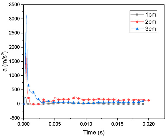
Figure 19.
Acceleration of wedges impacting different ice thicknesses.
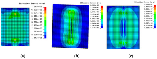
Figure 20.
Ice surface stress at maximum wedge acceleration. (a) h = 1 cm. (b) h = 2 cm. (c) h = 3 cm.
Figure 21 shows the final destruction state at 0.2 s. For the 1 cm thick ice, the ice is completely broken through but without significant deflection. The peak of acceleration is also smaller compared to the 2 cm and 3 cm thick ice, with the wedge hitting the 1 cm thick ice generating a peak acceleration of 229 m/s2. For the 2 cm thick ice, the wedge acceleration reaches 1963.24 m/s2; although the ice layer is not penetrated, it shows a significant deflection. For the 3 cm thick ice, the peak acceleration reaches 3203.06 m/s2.
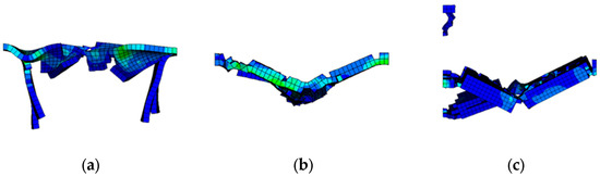
Figure 21.
Final damage state of ice sheets with different thicknesses. (a) h = 1 cm. (b) h = 2 cm. (c) h = 3 cm.
Due to the increase in thickness, the bending moment of the outer ice layer increases during the impact, causing fractures in the middle and outer regions of the ice layer. The degree of fracture is slightly more severe in the 3 cm ice than 2 cm ice, likely because the increase in the ice layer thickness is not significant. In addition, relative to the wedge, whose breakage speed is 10 m/s, the thickness–to–width ratio of the ice increases, leading to more brittle damage in the outer ice layer due to increased bending stress.
6.4. Different Objects Breaking through Ice into Water
This study simulates icebreaking using three different elements: a wedge, a cube, and a sphere. The side length of the cube and the diameter of the sphere are both 0.2 m, and the mass is 33.55 kg. The ice is 2 cm thick, and the icebreaking speed is 10 m/s. Figure 22 shows the acceleration curves of the three objects; they all exhibit the same trend, with the sphere having the lowest peak acceleration and the cube having the highest.
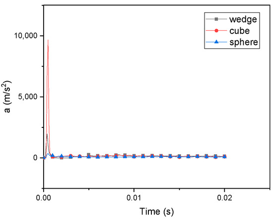
Figure 22.
Acceleration of different objects when breaking through ice.
As shown in Figure 23, during the specified calculation time, the sphere shows the largest deformation among the three objects. When the sphere impacts the ice surface, the energy is more evenly transferred to the ice layer, so the peak acceleration of the sphere is the lowest. The peak acceleration of the cube is the highest because it makes the largest contact area with the ice upon impact. Unlike the wedge and the sphere, there is no distinct depression in the center of the ice when the cube breaks, and the cracks extend outward from the center to the four sides, eventually breaking along the long side.

Figure 23.
Calculation of the final state of different objects when they break through the ice over time. (a) Wedge. (b) Cube. (c) Sphere.
7. Conclusions
In this study, a numerical model of wedge–ice–water interaction is constructed based on the commercial software LS–DYNA to simulate the process of wedge breaking through ice into water. The ALE method is used to track the gas–liquid interface and model the wedge breaking through ice and entering water. This study also discusses the effects of different impact velocities and wedge masses on the icebreaking process. The following conclusions are drawn:
- Numerical simulations of wedge ingress are carried out to simulate pool ingress tests. The feasibility of the ALE method for simulating structural ingress is verified by comparing acceleration data.
- Numerical simulations of a rigid plate impacting spherical ice are carried out. The feasibility of the numerical simulation method in structure–ice collisions is verified by comparison with P–A theoretical curves.
- The simulation shows that the destruction rate of ice is slower in the presence of water than in the absence of water, thus demonstrating that water can delay the destruction of ice.
- When the wedge mass is 23.55 kg and the impact velocity is increased from 10 to 30 m/s, greater impact velocities (e.g., 30 m/s) cause more pronounced ice destruction and greater damage acceleration.
- When the water entry speed is 10 m/s and the mass is 43.55 kg, the peak of acceleration is 1520 m/s2. It can be seen that the larger the mass of the wedge, the smaller the collision acceleration, though the effect on ice destruction is minimal.
- When the impact velocity is 10 m/s, the mass is 33.55 kg, and the ice thickness is 3 cm, the peak acceleration reaches 3202.06 m/s2. The acceleration of the wedge increases as the ice thickness increases.
Author Contributions
Conceptualization, Y.J. and F.W.; methodology, Y.J., F.W. and B.Q.; software, Z.Z., Y.L. and B.Q.; validation, Y.L. and Z.Z.; formal analysis, Y.J., F.W., L.M. and X.W.; investigation, Y.J., Y.L., Z.Z., L.M. and X.W.; resources, Y.J. and F.W.; data curation, Y.J., F.W., Y.L., Z.Z. and B.Q.; writing—original draft preparation, Y.J. and B.Q.; writing—review and editing, Y.J. and Y.L.; visualization, Y.L., Z.Z. and B.Q.; supervision, Y.J. and F.W.; project administration, Y.J.; funding acquisition, Y.J. All authors have read and agreed to the published version of the manuscript.
Funding
This study was supported by the Key Research and Development program of Shandong Province (2022CXGC020509), the Program of Yantai Science and Technology Innovation Development (2023XDRH018), and the program of KY10100230078 and 62602010322.
Institutional Review Board Statement
Not applicable.
Informed Consent Statement
Not applicable.
Data Availability Statement
The data used to support the findings of this study are available from the corresponding authors upon request.
Conflicts of Interest
Author Fucun Wang was employed by the Yantai Hongyuan Oxygen Industrial company. The remaining authors declare that the research was conducted in the absence of any commercial or financial relationships that could be construed as a potential conflict of interest.
References
- Patil, A.; Sand, B.; Fransson, L.; Bonath, V.; Cwirzen, A. Simulation of Brash Ice Behavior in the Gulf of Bothnia Using Smoothed Particle Hydrodynamics Formulation. J. Cold Reg. Eng. 2021, 35, 04021003. [Google Scholar] [CrossRef]
- Zhang, N.; Zheng, X.; Ma, Q.; Hu, Z. A Numerical Study on Ice Failure Process and Ice-Ship Interactions by Smoothed Particle Hydrodynamics. Int. J. Nav. Archit. Ocean Eng. 2019, 11, 796–808. [Google Scholar] [CrossRef]
- Liu, Y.; Qiao, Y.; Li, T. A Correct Smoothed Particle Method to Model Structure-Ice Interaction. CMES—Comput. Model. Eng. Sci. 2019, 120, 177–201. [Google Scholar] [CrossRef]
- Liu, M.; Wang, Q.; Lu, W. Peridynamic Simulation of Brittle-Ice Crushed by a Vertical Structure. Int. J. Nav. Archit. Ocean Eng. 2017, 9, 209–218. [Google Scholar] [CrossRef]
- Erceg, S.; Erceg, B.; von Bock und Polach, F.; Ehlers, S. A Simulation Approach for Local Ice Loads on Ship Structures in Level Ice. Mar. Struct. 2022, 81, 103117. [Google Scholar] [CrossRef]
- Ren, H.; Zhao, X. Numerical Simulation for Ice Breaking and Water Entry of Sphere. Ocean Eng. 2022, 243, 110198. [Google Scholar] [CrossRef]
- Wu, X.; Li, Y.; Cai, W.; Guo, K.; Zhu, L. Dynamic Responses and Energy Absorption of Sandwich Panel with Aluminium Honeycomb Core under Ice Wedge Impact. Int. J. Impact Eng. 2022, 162, 104137. [Google Scholar] [CrossRef]
- Bateman, S.P.; Orzech, M.D.; Calantoni, J. Simulating the Mechanics of Sea Ice Using the Discrete Element Method. Mech. Res. Commun. 2019, 99, 73–78. [Google Scholar] [CrossRef]
- Jang, H.K.; Kim, M.H. Kulluk-Shaped Arctic Floating Platform Interacting with Drifting Level Ice by Discrete Element Method. Ocean Eng. 2021, 236, 109479. [Google Scholar] [CrossRef]
- Jang, H.K.; Kim, M.H. Dynamics of Moored Arctic Spar Interacting with Drifting Level Ice Using Discrete Element Method. Ocean Syst. Eng. 2021, 11, 313–330. [Google Scholar] [CrossRef]
- Ji, S.; Wang, S. A Coupled Discrete-Finite Element Method for the Ice-Induced Vibrations of a Conical Jacket Platform with a GPU-Based Parallel Algorithm. Int. J. Comput. Methods 2020, 17, 1850147. [Google Scholar] [CrossRef]
- van den Berg, M.; Lubbad, R.; Løset, S. Repeatability of Ice-Tank Tests with Broken Ice. Mar. Struct. 2020, 74, 102827. [Google Scholar] [CrossRef]
- Zhu, H.; Ji, S. Discrete Element Simulations of Ice Load and Mooring Force on Moored Structure in Level Ice. CMES—Comput. Model. Eng. Sci. 2022, 132, 5–21. [Google Scholar] [CrossRef]
- Long, X.; Liu, S.; Ji, S. Discrete Element Modelling of Relationship between Ice Breaking Length and Ice Load on Conical Structure. Ocean Eng. 2020, 201, 107152. [Google Scholar] [CrossRef]
- Long, X.; Liu, S.; Ji, S. Breaking Characteristics of Ice Cover and Dynamic Ice Load on Upward–Downward Conical Structure Based on DEM Simulations. Comput. Part. Mech. 2021, 8, 297–313. [Google Scholar] [CrossRef]
- Jeong, S.Y.; Choi, K.; Kim, H.S. Investigation of Ship Resistance Characteristics under Pack Ice Conditions. Ocean Eng. 2021, 219, 108264. [Google Scholar] [CrossRef]
- Liu, L.; Ji, S. Comparison of Sphere-Based and Dilated-Polyhedron-Based Discrete Element Methods for the Analysis of Ship–Ice Interactions in Level Ice. Ocean Eng. 2022, 244, 110364. [Google Scholar] [CrossRef]
- Jou, O.; Celigueta, M.A.; Latorre, S.; Arrufat, F.; Oñate, E. A Bonded Discrete Element Method for Modeling Ship–Ice Interactions in Broken and Unbroken Sea Ice Fields. Comput. Part. Mech. 2019, 6, 739–765. [Google Scholar] [CrossRef]
- van den Berg, M.; Lubbad, R.; Løset, S. The Effect of Ice Floe Shape on the Load Experienced by Vertical-Sided Structures Interacting with a Broken Ice Field. Mar. Struct. 2019, 65, 229–248. [Google Scholar] [CrossRef]
- Huang, L.; Tuhkuri, J.; Igrec, B.; Li, M.; Stagonas, D.; Toffoli, A.; Cardiff, P.; Thomas, G. Ship resistance when operating in floating ice floes: A combined CFD&DEM approach. Mar. Struct. 2020, 74, 102817. [Google Scholar] [CrossRef]
- He, K.; Ni, B.; Xu, X.; Wei, H.; Xue, Y. Numerical Simulation on the Breakup of an Ice Sheet Induced by Regular Incident Waves. Appl. Ocean Res. 2022, 120, 103024. [Google Scholar] [CrossRef]
- Tang, X.; Zou, M.; Zou, Z.; Li, Z.; Zou, L. A Parametric Study on the Ice Resistance of a Ship Sailing in Pack Ice Based on CFD-DEM Method. Ocean Eng. 2022, 265, 112563. [Google Scholar] [CrossRef]
- Jeon, S.; Kim, Y. Numerical Simulation of Level Ice–Structure Interaction Using Damage-Based Erosion Model. Ocean Eng. 2021, 220, 108485. [Google Scholar] [CrossRef]
- Pernas-Sánchez, J.; Pedroche, D.A.; Varas, D.; López-Puente, J.; Zaera, R. Numerical Modeling of Ice Behavior under High Velocity Impacts. Int. J. Solids Struct. 2012, 49, 1919–1927. [Google Scholar] [CrossRef]
- Xu, Y.; Wu, J.; Li, P.; Kujala, P.; Hu, Z.; Chen, G. Investigation of the Fracture Mechanism of Level Ice with Extended Finite Element Method. Ocean Eng. 2022, 260, 112048. [Google Scholar] [CrossRef]
- He, Z.; Gao, Z.; Gu, X.; Gao, Z. Numerical simulation on the structural response of a torpedo at the moment of vertical water entry. Explos. Shock. Waves 2023, 43, 073303. [Google Scholar] [CrossRef]
- Wang, C.; Wang, J.; Wang, C.; Guo, C.; Zhu, G. Research on vertical movement of cylindrical structure out of water and breaking through ice layer based on S-ALE method. Chin. J. Theor. Appl. Mech. 2021, 53, 3110–3123. [Google Scholar] [CrossRef]
- Hallquist, O.J. Theory Manual; Livermore Software Technology Corporation LS_DYNA 2006: Livermore, CA, USA, 2006. [Google Scholar]
- Anghileri, M.; Castelletti, L.M.L.; Invernizzi, F.; Mascheroni, M. A survey of numerical models for hail impact analysis using explicit finite element codes. Int. J. Impact Eng. 2005, 31, 929–944. [Google Scholar] [CrossRef]
- Masterson, D.M.; Frederking, R.M.W.; Wright, B.; Karna, T.; Maddock, W.P. A revised ice pressure-areacurve. In Proceedings of the 19th International Conference on Port and Ocean Engineering under Arctic Conditions, Dalian, China, 27–30 June 2007; Volume 1, pp. 305–314. [Google Scholar]
Disclaimer/Publisher’s Note: The statements, opinions and data contained in all publications are solely those of the individual author(s) and contributor(s) and not of MDPI and/or the editor(s). MDPI and/or the editor(s) disclaim responsibility for any injury to people or property resulting from any ideas, methods, instructions or products referred to in the content. |
© 2024 by the authors. Licensee MDPI, Basel, Switzerland. This article is an open access article distributed under the terms and conditions of the Creative Commons Attribution (CC BY) license (https://creativecommons.org/licenses/by/4.0/).