Abstract
The determination of the optimal random field element (RFE) size is crucial in soil slope reliability analysis as it governs the trade-off between precision in failure probability calculations and computational efficiency. Given the substantial computational burden associated with smaller RFE sizes, studies on their impact on slope failure probability are scarce. This research examines the influence of RFE size on failure probability and safety factor, employing the Karhunen–Loève expansion to generate random fields and integrating the simplified Bishop method with particle swarm optimization (PSO) to assess slope stability. Through Monte Carlo Simulation (MCS), this study investigates the effects of the ratio of slope height to RFE size (H/De) on slope reliability metrics across two illustrative cases. Results reveal a notable influence of H/De on the distribution of safety factors (Fs) and failure probability (PF), with overestimation observed at smaller H/De ratios. When H/De exceeds 10 for Example 1 and 15 for Example 2, the Fs distribution patterns in both scenarios stabilize significantly, displaying minimal variability. The PF of Example 1 and Example 2 decreases with the increase of H/De and remains basically unchanged when H/De exceeds 10 and 15, respectively. Consequently, a recommended H/De ratio of 20 is proposed based on the analyzed cases, facilitating accurate calculations while mitigating computational overhead.
1. Introduction
Slope stability analysis is a key research area in geotechnical engineering. Large-scale landslides can bury houses and factories, disrupt traffic, and block rivers, posing severe threats to people’s lives and property safety [1]. Assessing slope stability is vital for ensuring the safety and reliability of civil engineering projects. The deterministic approaches employed in assessing slope stability encompass various methodologies, notably including the finite element analysis method (FEAM) [2,3,4], limit analysis method (LAM) [5,6], and limit equilibrium method (LEM) [7,8,9]. The LEM is simple in principle and calculation and can obtain reliable results. Therefore, the LEM has garnered widespread adoption in the assessment of soil slope stability.
Nonetheless, the uncertainties inherent in geotechnical engineering exert a profound influence on the reliability of slope stability, consequently leading to potential unreliability in the deterministic analyses [10]. Among these uncertainties, the spatial variability of soil properties stands out as a pivotal factor, constituting one of the key uncertainties affecting slope stability [11,12,13]. Although soil parameters can be determined through geotechnical testing, achieving accurate assessments for each specific location remains infeasible. Therefore, in the context of slope reliability analysis, random field theory assumes considerable significance as an effective means for characterizing the spatial variability of soil parameters [13,14]. The Karhunen–Loève (KL) expansion is recognized as one of the methodologies for generating random fields. This technique is widely utilized by numerous researchers [14,15] due to its ability to achieve the same accuracy requirements with a lesser number of expansion terms.
Over the past few years, increasing attention has been paid to the reliability analysis of slopes considering the uncertainties of soil parameters [15,16,17]. Cho [14] presented the Random Limit Equilibrium Method (RLEM), an innovative approach that harmonizes random field theory with the well-established LEM. This integration results in a robust methodology particularly suited to assessing the reliability of soil slope designs. Then, the RLEM was used by various researchers to study the probability of the saturated slope [18], the slope considering the nonlinear failure criterion [16], the slope reinforced permeable polymer [19], and the three dimensional slope [15]. Taking into account the spatial variability of soil parameters, slope reliability analysis can become exceedingly time-consuming [20]. When employing RLEM for slope reliability analysis, a substantial number of numerical simulations must be conducted, with each simulation requiring the determination of the critical slip surface (CSS). Hence, one of the keys to increasing the efficiency of reliability analysis lies in effectively reducing the time needed to determine the CSS of the slope [21]. The Particle Swarm Optimization (PSO) method has been employed by numerous researchers for identifying the CSS of slope [22] owing to its advantages of simple operation, high computational efficiency, and robust stability [23,24,25]. When applying the RLEM for slope reliability analysis, the random field is discretized into elements of specific dimensions to characterize the spatial variability of soil. The random field element (RFE) size plays a crucial role in the slope reliability analysis [26]. A larger RFE size may inadequately describe the spatial variability of soil parameters, negatively impacting slope reliability analysis results. Conversely, a smaller RFE size can better describe this variability but may also introduce significant computational demands [26]. It is very important to determine the appropriate RFE size in slope reliability analysis, yet it remains a topic that has garnered limited attention from scholars.
The primary objective of this study is to conduct a thorough analysis of the influence of RFE size on slope reliability. To achieve this, the K-L expansion method is employed to generate random fields for soil parameters, and an integration of RLEM with the PSO algorithm is utilized to ascertain the CSS of slopes precisely. The Monte Carlo Simulation (MCS) method is applied to compute the failure probability of the slopes. Ultimately, this study will focus on analyzing the crucial role of the H/De ratio in slope reliability analysis, providing valuable insights for related fields.
2. Methods
2.1. Karhunen–Loève (KL) Method
The characteristics of a random field are defined by its mean μ, standard deviation σ, and autocorrelation function [14]. In this study, the adopted autocorrelation function expression is formulated as follows:
where τx and τy are the relative separation distances along the x-axis and y-axis, respectively, while δx and δy denote the corresponding fluctuation ranges along these axes.
The cohesion (c) and friction angle (φ) are considered to be the uncertain characteristics of soil, exhibiting a close and inseparable interdependence that cannot be ignored. The cross-correlated lognormal random fields can be represented as follows [21]:
where χi(θ) is random variable; λi and φi(x) are the eigenvalues and eigenfunctions of the autocorrelation function, respectively; M is the truncation term of the series expansion; μln = lnμ − (σln)2/2 and σln = (ln(1 + (σ/μ)2))0.5 are the mean and standard deviation of lognormal random field, respectively; and ρc,φ is the cross correlation coefficient between c and φ.
2.2. Bishop’s Method
Compared to rigorous analytical methods, Bishop’s method can yield very accurate results [27]. Therefore, this study employs this method, and the factor of safety Fs can be expressed as
in which
where Wi is the weight of soil slice, μi is the pore water pressure, and αi is the inclination of the bottom.
Wan et al. [21] optimized the PSO algorithm to enhance the computational efficiency in determining the CSS of slope. This study adopts the improved PSO method to determine the CSS of slope.
2.3. Estimation of Failure Probability of Slope
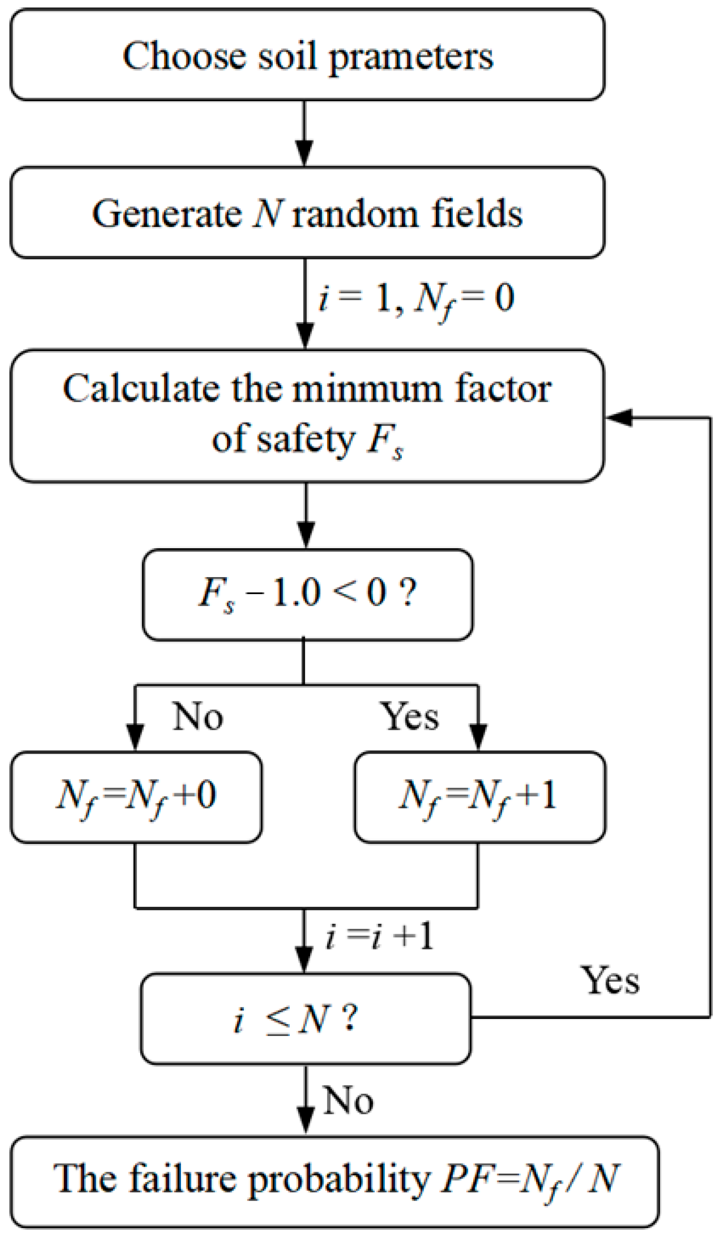
To assess the failure probability (PF) of a slope, an MCS is performed. The algorithmic approach employed for computing PF is shown in Figure 1.
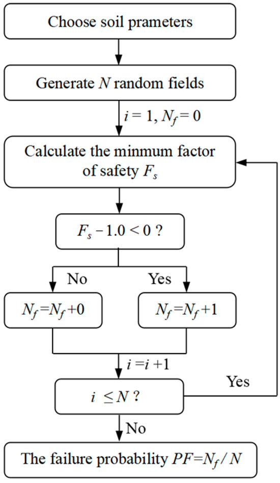
Figure 1.
Flow chart for computing PF.
3. Results and Discussion
In this study, an approximate relative error (RE) is used to study the impact of RFE size on the PF. Considering the slope discretized into square elements, each with a width denoted as De = w1, w2, w3…wn, where w1 represents the minimum value among w1, w2, w3…wn and is deemed sufficiently small. Thus, the RE pertaining to PF can be formulated as follows:
where PF1 is the PF with De = w1, and PFi is the PF with De = wi. The critical dimension of RFE corresponds to the minimum size at which any further decrement in De fails to elicit a notable reduction in the absolute RE of PF, thereby indicating the optimal balance between accuracy and computational efficiency.
This study utilizes an analysis program that was developed by the author using the MATLAB programming language (R2020a, 9.8.0).
Example 1:
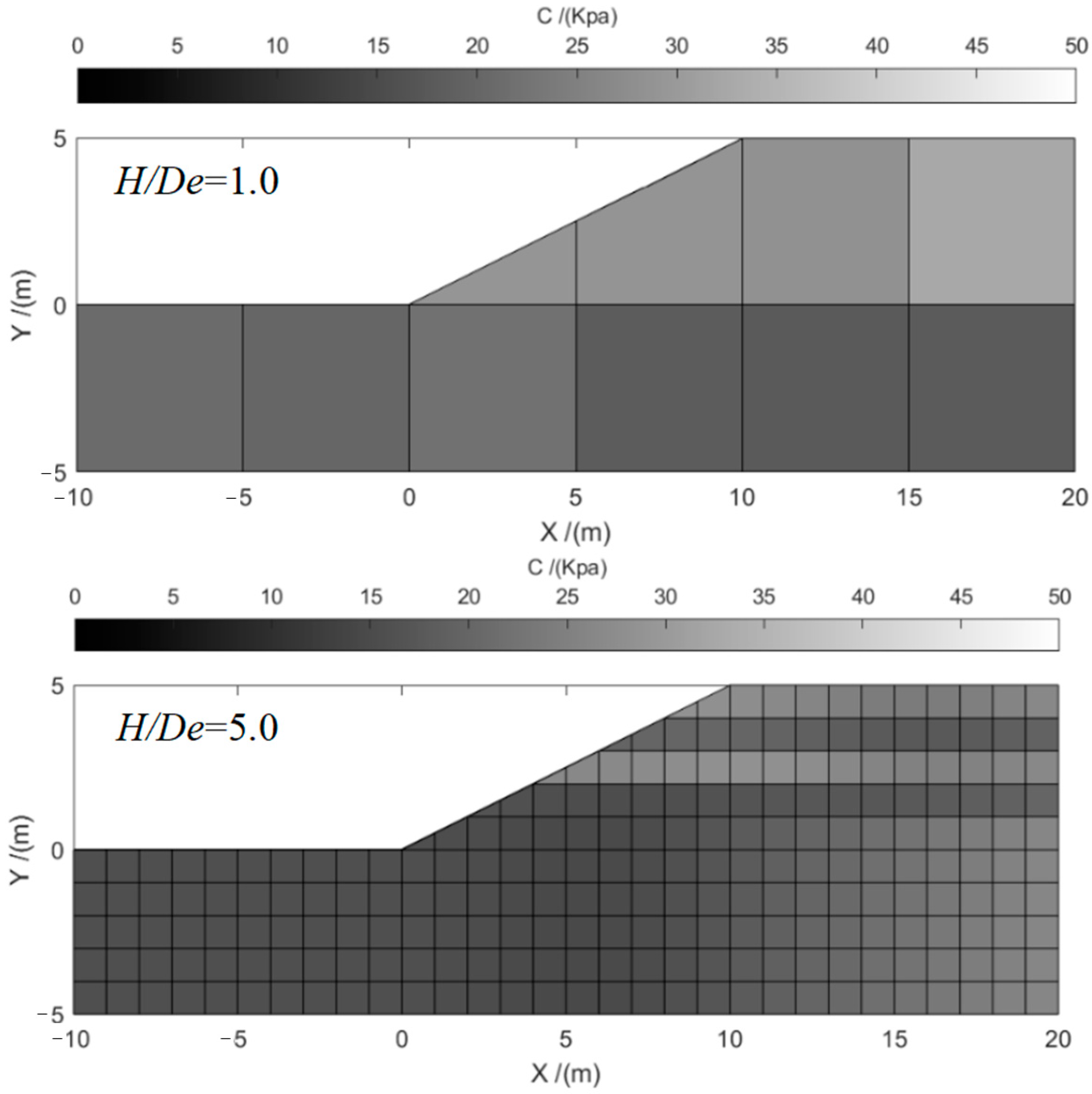
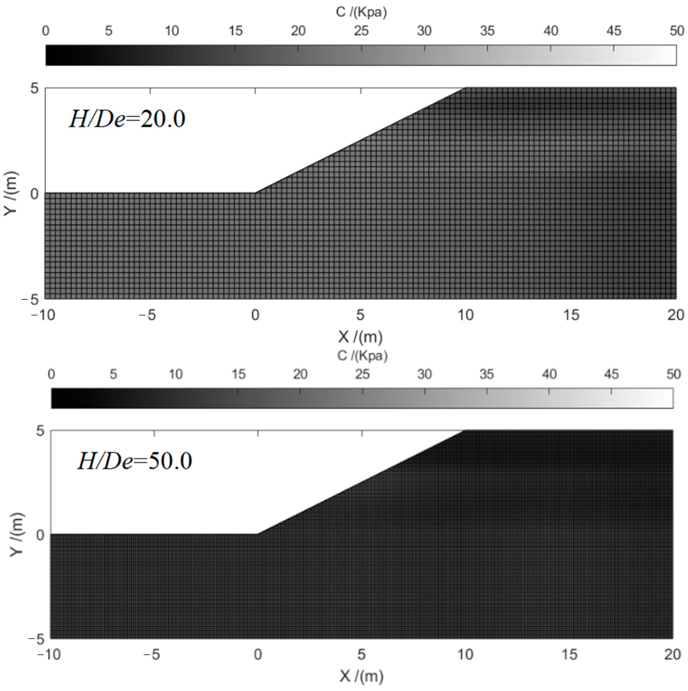
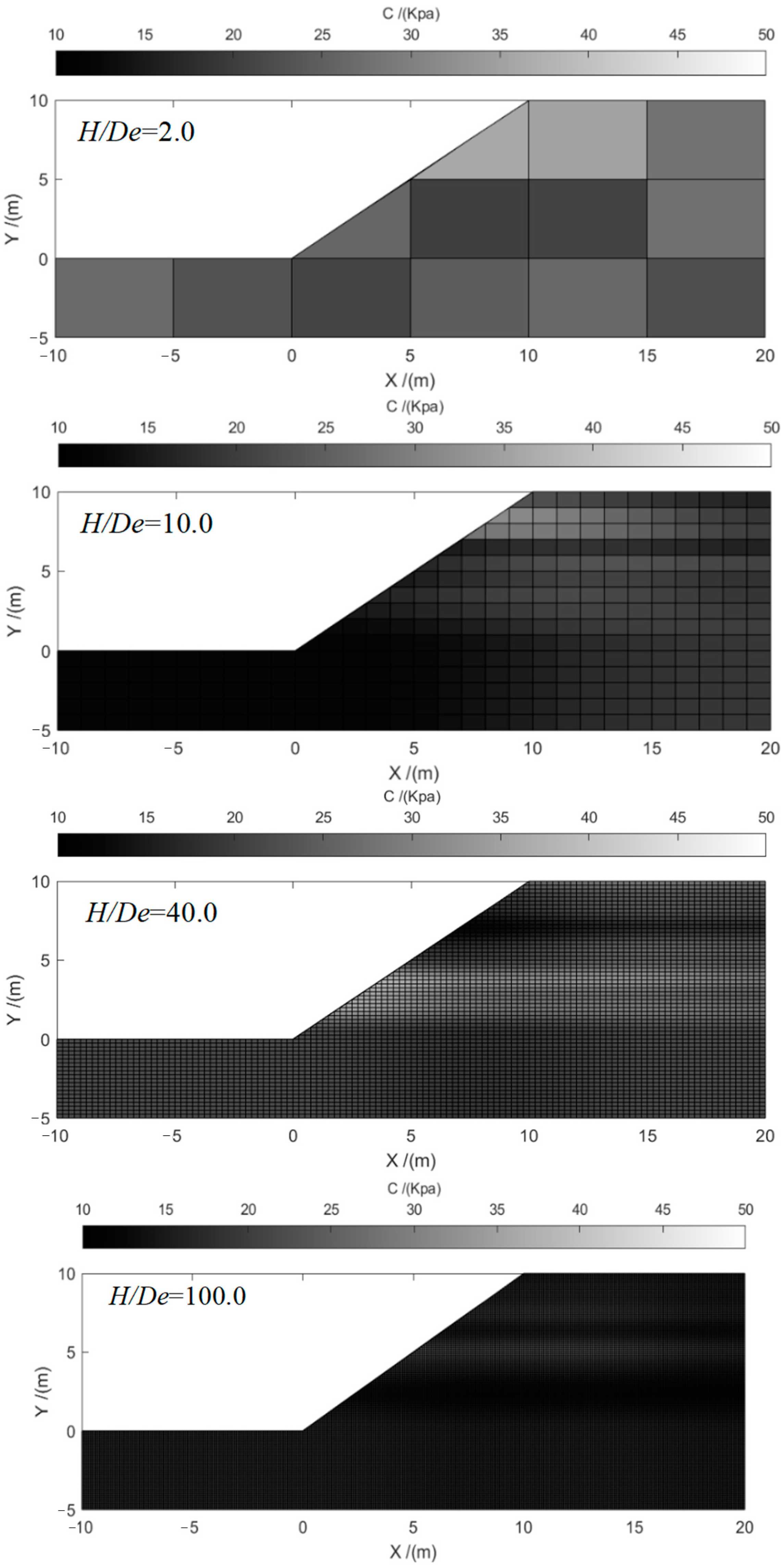
Example 1 proposed by Cho [14] is typical slope with single layer undrained cohesive. Table 1 displays the soil parameters for Example 1, including the mean (μc) and covariance (COVc) of c and the soil weight (γ), mean (μφ), and covariance (COVφ) of φ. This study considered the scenarios with constant δh (δh = 40 m) and different δv (δv = 3 m, 5 m, 7 m). In this example, we modeled the shear strength c as a random field using the K-L expansion method with different RFE sizes; De = 10 m, 5.0 m, 2.5 m, 1.0 m, 0.5 m, 0.25 m, 0.2 m, 0.15 m, 0.1 m, 0.09 m, and 0.08 m. And the corresponding ratios of slope height and RFE size (H/De) are 0.5, 1, 2, 5, 10, 20, 25, 33, 50, 55, and 62.5, respectively. When employing the MCS for slope reliability analysis, the accuracy of the results improves with the increasing number of simulations. Typically, a relatively accurate result can be obtained after 10,000 simulations. To ensure the precision of the computational outcomes in this study, we generated 50,000 random field realizations using MCS. Figure 2 shows the typical random field realization by the RFE size of 5 m, 1 m, 0.25 m, and 0.1 m, respectively.

Table 1.
Soil parameters in two examples.
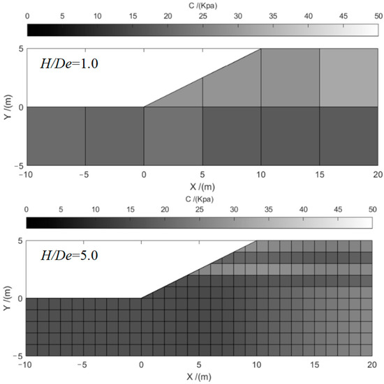
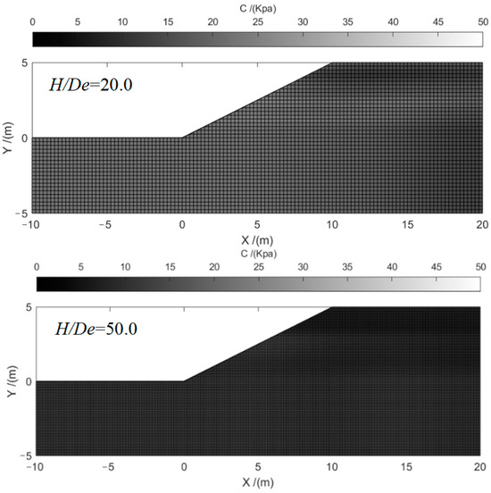
Figure 2.
Typical random field realization with RFE sizes De = 5 m, 1 m, 0.25 m, and 0.1 m of Example 1.
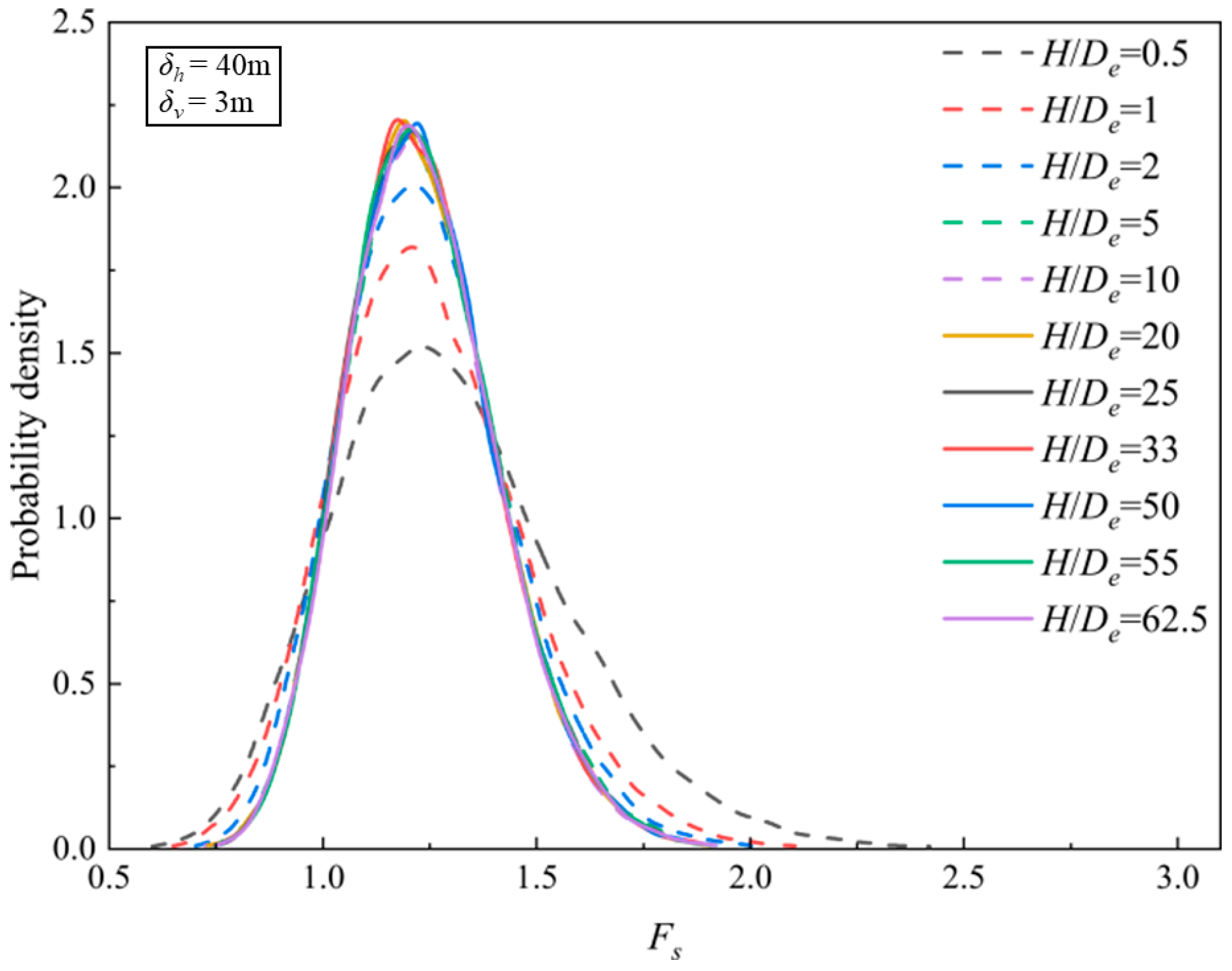
In this section, the effects of the REF size on Fs is analyzed. Figure 3 illustrates the distribution of Fs for various H/De of Example 1. The Fs corresponding the maximum probability density function value is around 1.25. It can be seen that when H/De is smaller than 5, the probability density of Fs becomes higher, and the distribution of Fs becomes more and more concentrated at 1.25 with the increase in H/De. Nevertheless, when the element has a relatively smaller size like H/De > 10, the distribution of Fs tends to be stable without much change.
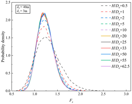
Figure 3.
Distribution of the Fs for different H/De ratios with δh = 40 m and δv = 3 m in Example 1.
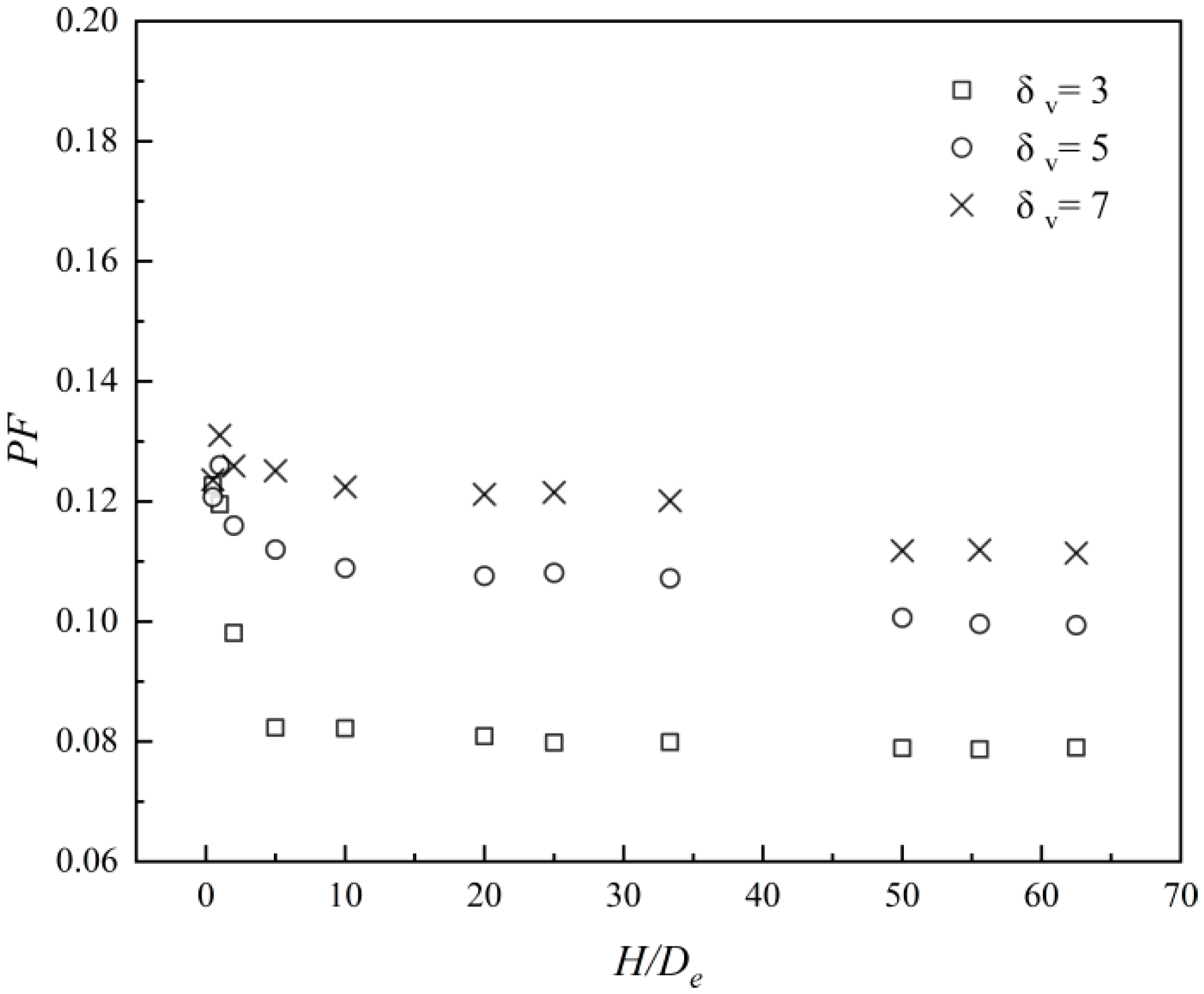
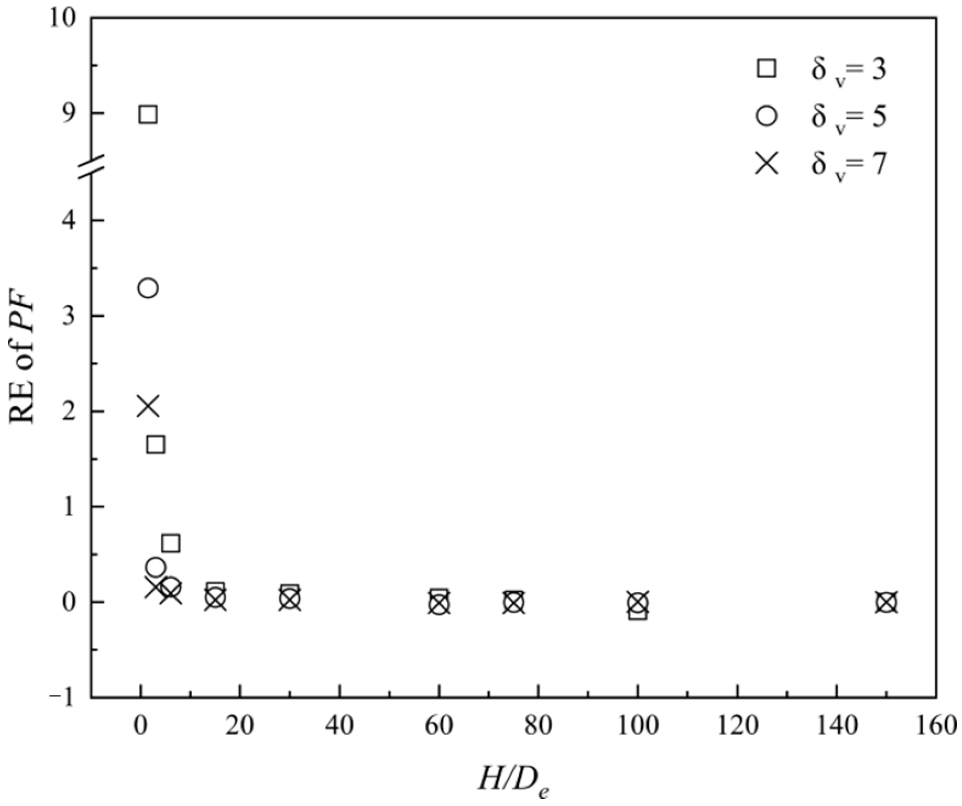
The effect of the RFE size on the PF of slopes was analyzed in this section. Figure 4 and Figure 5 show the PF values for various H/De. As shown in Figure 4, when the RFE size De is large and H/De is small, the value of PF was obviously overestimated, and as De decreases and H/De increases, it shows a downward trend and gradually becomes a steady state. This is because when the RFE size is relatively large, the number of elements into which the slope is divided is smaller, making the slope appear relatively homogeneous. This means that the c values at different locations are very similar. Therefore, the average c at the slip surface has a relatively high probability to take a very low value. But when the De value is large, this phenomenon will be reversed due to the influence of spatial averaging. When RFE size is small, the number of elements would be large, and the realization of the c field would be heterogeneous. It means that the value of c at different locations are likely to be different, and the smaller c at one point could be offset by a larger value at another point. Thus, the failure probability would be overestimated by a large RFE size and a small H/De. Figure 5 illustrates the RE of PF, as the RFE size decreases, the relative error of PF also decreases and gradually stabilizes, and finally no longer decreases and approaches 0.
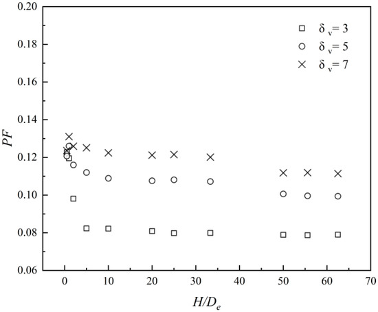
Figure 4.
Effect of the different H/De ratios and δv on statistics of PF in Example 1.
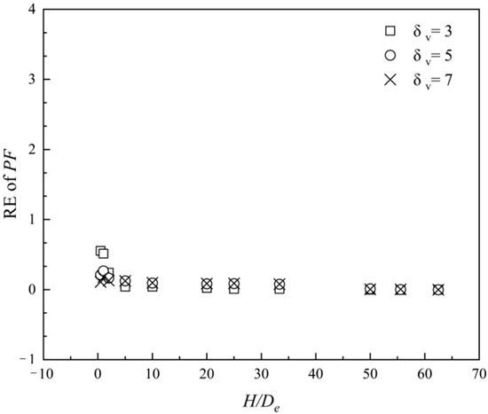
Figure 5.
Effect of the different H/De ratios and δv on the relative error of probability of failure PF in Example 2.
Example 2:
Example 2, proposed by Cho [14], is an c-φ slope. The property parameters associated with this slope are presented in Table 1, and δv and δh are the same as in Example 1. De is set to 10 m, 5.0 m, 2.5 m, 1.0 m, 0.5 m, 0.25 m, 0.2 m, 0.15 m, and 0.1 m, and the corresponding H/De is equal to 1.5, 3, 6, 15, 30, 60, 75, 100, and 150, respectively. Figure 6 shows the typical random field realization with De = 5 m, 1 m, 0.25 m, and 0.1 m.

Figure 6.
Typical random field realization with RFE sizes De = 5 m, 1 m, 0.25 m, and 0.1 m of Example 2.
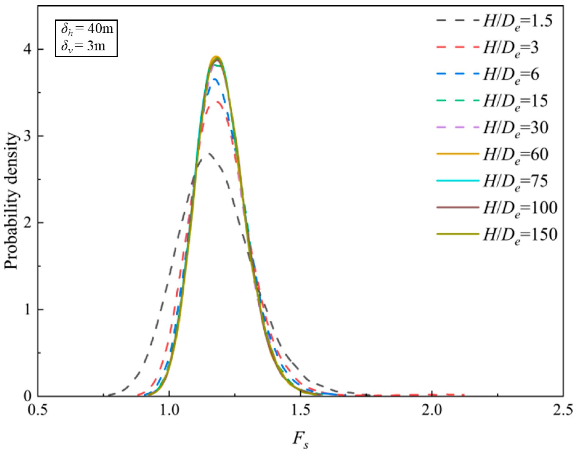
The distribution of Fs was similar to Example 1, as shown in Figure 7. When H/De is larger than 15, the distribution of FS becomes lightly flat. And when H/De is less than 15, with the increase in H/De, the distribution of Fs is more and more concentrated at 1.3. When H/De = 15, the distribution of Fs reaches the most concentrated state. As H/De continues to increase, the improvement in the distribution concentration state is no longer obvious.
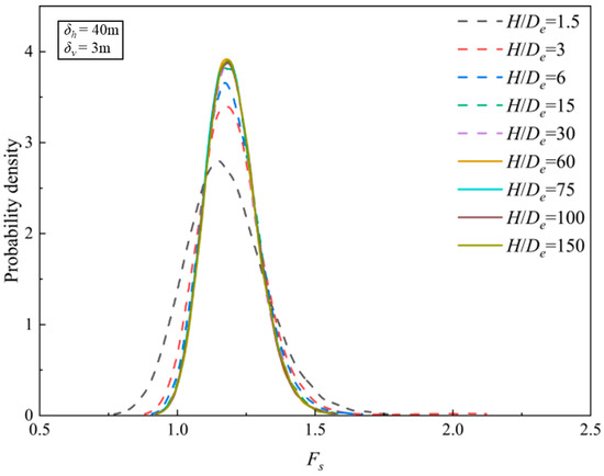
Figure 7.
Distribution of the Fs for different H/De ratios with δh = 40 m and δv = 3 m in Example 2.
Figure 8 plots the failure probability for various H/De and δv. The PF decreases rapidly as H/De increases when H/De < 15 and maintains a stable state of an approximately straight line after H/De > 15. And when H/De is the same, different δv will also have a significant impact on Fs. It can be found that the PF becomes smaller with the decrease in δv. Figure 9 illustrates the RE of PF; as the RFE size decreases, the relative error of PF also decreases and gradually stabilizes and finally no longer decreases and approaches 0. The results of Example 1 and Example 2 indicate that a critical ratio H/De = 20 emerges as pivotal in accurately assessing the probability of slope failure. This critical ratio signifies the optimal balance between precision and efficiency in slope stability analysis.
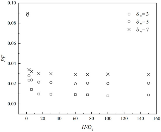
Figure 8.
Effect of the different H/De ratios and δv on statistics of PF in Example 2.
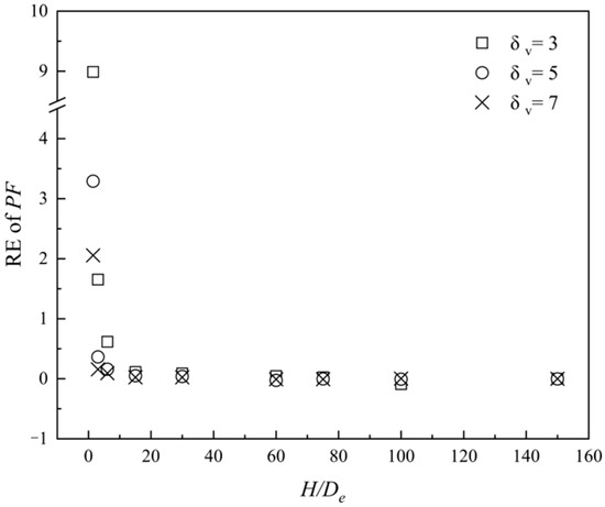
Figure 9.
Effect of the H/De ratio on the relative error of probability of failure PF in Example 2.
4. Conclusions
In this study, a reliability calculation program taking into account the spatial variability of soil parameters was presented. Based on the program, the impact of H/De on PF and Fs is analyzed. The following conclusions can be drawn:
The H/De has significant influence on the distribution of Fs. When H/De is less than 10, the distribution of Fs becomes more concentrated as H/De increases; when H/De is greater than 10, the distribution of Fs becomes very close as the grid size increases.
The H/De has significant influence on PF. The PF decreases with the increase in H/De and gradually tends to remain unchanged. When the value of H/De is small, it may lead to an overestimation of PF. This phenomenon underscores the importance of selecting an appropriate value for H/De to ensure accurate assessment of slope stability and avoid misleading results.
The results show that when the H/De exceeds 10 and 15 in Examples 1 and 2, respectively, PF remains essentially unchanged, which indicates that setting H/De to 20 can not only ensure the accuracy of calculations but also prevent the unnecessary consumption of computing resources.
This study focuses on the influence of H/De on computational accuracy. In order to obtain relatively stable computation results, this study has adopted more conservative parameter settings for both the number of MCS and the iterations of PSO. Reducing the number of MCS while maintaining computational accuracy, as well as rapidly searching for the CSS, are two crucial research directions for optimizing the computational strategy of slope reliability, warranting further investigation.
Author Contributions
Conceptualization, J.S.; methodology, Y.W.; software, H.G.; validation, H.G. and B.S.; data curation, J.S.; writing—original draft preparation, J.S.; visualization, B.S.; funding acquisition, Y.W. All authors have read and agreed to the published version of the manuscript.
Funding
This research was financially supported by grants of the Key R&D Program Project of Ningxia (No. 2022BEG03052), the Natural Science Foundation of Ningxia (2023AAC03036), and Ningxia Teaching Reform Project (Reform and Practice of “Photogrammetry and Remote Sensing” Course Teaching Based on School-Enterprise Cooperation).
Institutional Review Board Statement
Not applicable.
Informed Consent Statement
Not applicable.
Data Availability Statement
The raw data supporting the conclusions of this article will be made available by the authors on request.
Conflicts of Interest
The authors declare no conflicts of interest.
References
- Kasama, K.; Furukawa, Z.; Hu, L. Practical reliability analysis for earthquake-induced 3D landslide using stochastic response surface method. Comput. Geotech. 2021, 137, 104303. [Google Scholar] [CrossRef]
- Wei, W.; Tang, H.; Song, X.; Ye, X. 3D slope stability analysis considering strength anisotropy by a micro-structure tensor enhanced elasto-plastic finite element method. J. Rock. Mech. Geotech. 2024, in press. [Google Scholar] [CrossRef]
- Sheng, T.; Li, T.; Liu, X.; Qi, H. A Partitioned Rigid-Element and Interface-Element Method for Rock-Slope-Stability Analysis. Appl. Sci. 2023, 13, 7301. [Google Scholar] [CrossRef]
- Ke, L.; Gao, Y.; Fei, K.; Gu, Y.; Ji, J. Determination of depth-dependent undrained shear strength of structured marine clays based on large deformation finite element analysis of T-bar penetrations. Comput. Geotech. 2024, 176, 106758. [Google Scholar] [CrossRef]
- Li, D.; Jia, W.; Zhao, L.; Cheng, X.; Zhang, Y.; Fu, H.; Ye, B.; Zheng, L. Upper-bound limit analysis of rock slope stability with tensile strength cutoff based on the optimization strategy of dividing the tension zone and shear zone. Int. J. Geomech. 2022, 22, 6022006. [Google Scholar] [CrossRef]
- Zhang, H.; Li, C.; Chen, W.; Xie, N.; Wang, G.; Yao, W.; Jiang, X.; Long, J. Upper-bound limit analysis of the multi-layer slope stability and failure mode based on generalized horizontal slice method. J. Earth Sci. 2024, 35, 929–940. [Google Scholar] [CrossRef]
- Dai, G.; Gao, Y.; Zhang, F.; Shu, S. Stability of layered soil slope with tension crack: A closed-form solution. Can. Geotech. J. 2023, 61, 328–343. [Google Scholar] [CrossRef]
- Ouyang, W.; Liu, S.; Yang, Y. An improved morgenstern-price method using gaussian quadrature. Comput. Geotech. 2022, 148, 104754. [Google Scholar] [CrossRef]
- Zhang, F.; Ge, B.; Leshchinsky, D.; Shu, S.; Gao, Y. Effects of multitiered configuration on the internal stability of GRS walls. J. Geotech. Geoenviron. Eng. 2023, 149, 4023122. [Google Scholar] [CrossRef]
- Vanneschi, C.; Eyre, M.; Burda, J.; Zizka, L.; Francioni, M.; Coggan, J.S. Investigation of landslide failure mechanisms adjacent to lignite mining operations in North Bohemia (Czech Republic) through a limit equilibrium/finite element modelling approach. Geomorphology 2018, 320, 142–153. [Google Scholar] [CrossRef]
- Kalantari, A.R.; Johari, A.; Zandpour, M.; Kalantari, M. Effect of spatial variability of soil properties and geostatistical conditional simulation on reliability characteristics and critical slip surfaces of soil slopes. Transp. Geotech. 2023, 39, 100933. [Google Scholar] [CrossRef]
- Savvides, A.; Papadrakakis, M. Uncertainty quantification of failure of shallow foundation on clayey soils with a modified cam-clay yield criterion and stochastic fem. Geotechnics 2022, 2, 348–384. [Google Scholar] [CrossRef]
- Savvides, A.A.; Papadrakakis, M. A computational study on the uncertainty quantification of failure of clays with a modified Cam-Clay yield criterion. SN Appl. Sci. 2021, 3, 659. [Google Scholar] [CrossRef]
- Cho, S.E. Probabilistic Assessment of Slope Stability That Considers the Spatial Variability of Soil Properties. J. Geotech. Geoenviron. Eng. 2010, 136, 975–984. [Google Scholar] [CrossRef]
- Wang, Y.; Shao, L.; Wan, Y.; Chen, H. Reliability analysis of three-dimensional reinforced slope considering the spatial variability in soil parameters. Stoch. Environ. Res. Risk Assess. 2024, 38, 1583–1596. [Google Scholar] [CrossRef]
- Wan, Y.; Gao, X.; Wu, D.; Zhu, L.; Glade, T.; Murty, T.S. Reliability of spatially variable soil slope based on nonlinear failure criterion. Nat. Hazards 2023, 117, 1179–1189. [Google Scholar] [CrossRef]
- Dong-Ping, D.; Liang, L.; Lian-Heng, Z. Limit-Equilibrium Method for Reinforced Slope Stability and Optimum Design of Antislide Micropile Parameters. Int. J. Geomech. 2017, 17, 6016011–6016019. [Google Scholar] [CrossRef]
- Javankhoshdel, S.; Cami, B.; Chenari, R.J.; Dastpak, P. Probabilistic analysis of slopes with linearly increasing undrained shear strength using RLEM approach. Transp. Infrastruct. Geotechnol. 2021, 8, 114–141. [Google Scholar] [CrossRef]
- Wang, Y.; Shao, L.; Jiang, R.Y.X.W. Three-dimensional reliability stability analysis of earth-rock dam slopes reinforced with permeable polymer. Probabilist Eng. Mech. 2023, 74, 1. [Google Scholar] [CrossRef]
- Liu, L.; Deng, Z.; Zhang, S.; Cheng, Y. Simplified framework for system reliability analysis of slopes in spatially variable soils. Eng. Geol. 2018, 239, 330–343. [Google Scholar] [CrossRef]
- Wan, Y.; Xu, R.; Yang, R.; Zhu, L. Application of the improved particle swarm optimization method in slope probability analysis. Mar. Georesour Geotec. 2023, 42, 1531–1541. [Google Scholar] [CrossRef]
- Cheng, Y.M.; Li, L.; Chi, S.; Wei, W.B. Particle swarm optimization algorithm for the location of the critical non-circular failure surface in two-dimensional slope stability analysis. Comput. Geotech. 2007, 34, 92–103. [Google Scholar] [CrossRef]
- Zou, J.; Chen, H.; Jiang, Y.; Zhang, W.; Liu, A. An effective method for real-time estimation of slope stability with numerical back analysis based on particle swarm optimization. Appl. Rheol. 2023, 33, 20220143. [Google Scholar] [CrossRef]
- Himanshu, N.; Burman, A. Determination of critical failure surface of slopes using particle swarm optimization technique considering seepage and seismic loading. Geotech. Geol. Eng. 2019, 37, 1261–1281. [Google Scholar] [CrossRef]
- Shinoda, M.; Miyata, Y. PSO-based stability analysis of unreinforced and reinforced soil slopes using non-circular slip surface. Acta Geotech. 2018, 14, 907–919. [Google Scholar] [CrossRef]
- Yang, Z.; Nie, J.; Peng, X.; Tang, D.; Li, X. Effect of random field element size on reliability and risk assessment of soil slopes. B Eng. Geol. Environ. 2021, 80, 7423–7439. [Google Scholar] [CrossRef]
- Spencer, E. A method of analysis of the stability of embankments assuming parallel inter-slice forces. Geotechnique 1967, 17, 11–26. [Google Scholar] [CrossRef]


Disclaimer/Publisher’s Note: The statements, opinions and data contained in all publications are solely those of the individual author(s) and contributor(s) and not of MDPI and/or the editor(s). MDPI and/or the editor(s) disclaim responsibility for any injury to people or property resulting from any ideas, methods, instructions or products referred to in the content. |
© 2024 by the authors. Licensee MDPI, Basel, Switzerland. This article is an open access article distributed under the terms and conditions of the Creative Commons Attribution (CC BY) license (https://creativecommons.org/licenses/by/4.0/).