Fully Automatic Grayscale Image Segmentation: Dynamic Thresholding for Background Adaptation, Improved Image Center Point Selection, and Noise-Resilient Start/End Point Determination

Abstract

As the requirement for image uploads in various systems continues to grow, image segmentation has become a critical task for subsequent operations. Balancing the efficiency and accuracy of image segmentation is a persistent challenge. This paper focuses on threshold-based grayscale image segmentation methods and proposes a fully automated approach. The approach begins with the implementation of an improved OTSU algorithm to determine the optimal dynamic threshold, enabling the segmentation process to adjust adaptively to varying image backgrounds. A novel method for selecting image center points is introduced to address the issue of poor segmentation when the center point falls outside the segmentation foreground area. To further enhance the algorithm’s generalization capability and accuracy, a continuity detection-based method is developed to determine the start and end points of the segmentation foreground. Compared with traditional algorithms, tests on sample images of four different scales revealed that the proposed algorithm achieved average improvements in accuracy, precision, and recall rates of 14.97%, 1.28%, and 17.33%, respectively, with processing speed remaining largely unaffected. Ablation experiments further validated the effectiveness of using different strategy combinations, with the combination of all three strategies resulting in significant improvements in accuracy and recall rates by 15.51% and 16.72%, respectively.

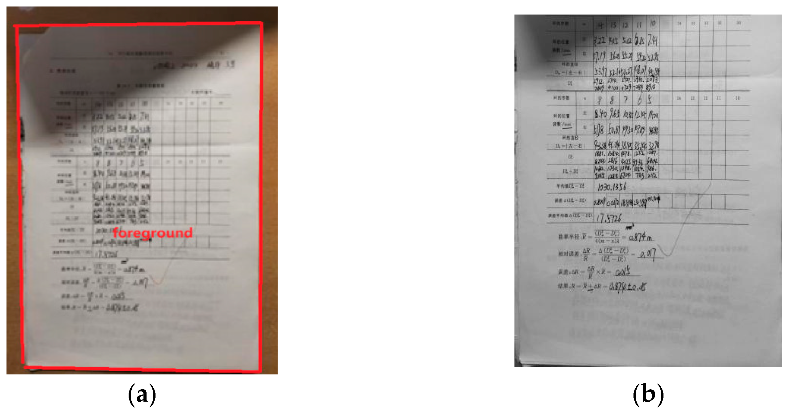
1. Introduction

With the advancements in mobile internet technology, there is a growing demand for systems capable of uploading images across various application scenarios. Once these images are uploaded to the server, they are first converted to grayscale, followed by image segmentation to extract the effective region from the original image, thereby facilitating subsequent processing (Figure 1) [1].

Image segmentation technology is a crucial component in computer vision, serving as the foundation for numerous applications, including object recognition and understanding [2], medical imaging [3], autonomous systems and robotics [4,5], augmented reality [6], virtual reality [7], video surveillance and security [8,9], as well as environmental monitoring and agriculture [10]. However, image segmentation under complex background conditions remains challenging due to factors such as noise interference, uneven lighting, and blurred target edges [11,12].

Figure 1. The original images to be processed [13].

Figure 1. The original images to be processed [13].

Image segmentation algorithms can be categorized into four primary techniques based on different processing methods: threshold-based segmentation [14], edge-based segmentation [15], region-based segmentation [16], and theory-based segmentation [17]. This paper focuses on threshold-based image segmentation methods, which utilize grayscale information and threshold extraction to segment images by setting one or more thresholds that classify pixels into different categories, effectively separating the background from the foreground [18]. Threshold-based segmentation is widely used in image processing today, offering several advantages, including stable performance, simple models, and ease of implementation. It is extensively applied across various fields of image segmentation processing [19,20,21,22].

In complex images, the differences between the target and background regions necessitate the selection of an optimal threshold for image segmentation, which divides the image into target and background areas. The effectiveness of segmentation is directly influenced by the choice of this optimal threshold. Extensive research has been conducted on this issue, with scholars introducing meta-heuristic algorithms (MAs) to optimize processing and improve segmentation accuracy [23]. Tian Miao et al. [24] proposed a rapid extraction method for iterative threshold segmentation, enhancing algorithm accuracy. Jiwei Lang et al. [25] utilized manual threshold adjustment to ensure optimal image segmentation results. Neha Singh [26] introduced a variational mode decomposition (VMD) method that employs the OTSU algorithm to determine the optimal threshold, providing precision while overcoming the limitations of fixed thresholds. K. M. Hosn [27] introduced the concept of chaotic mapping to optimize the initialization step, while L. Abualigah [28] proposed the Salp Swarm Algorithm (SSA) to determine optimal multi-level thresholds. Abdel-Basset [29] applied the improved whale optimization algorithm (IWOA) to solve the multi-threshold segmentation of grayscale images. Yaobin Zou [30] proposed a Tsallis entropy threshold segmentation method based on multi-scale and multi-directional Gabor transformation. Naik et al. [31] utilized the equilibrium slime mould algorithm (ESMA) to search for multi-level thresholds using the entropy method, significantly improving segmentation accuracy. Abdel-KHALEK [32] proposed a novel image segmentation method based on genetic algorithms (GA) and entropy to enhance image segmentation quality. Shubham [33] further improved this by proposing a new multi-level threshold criterion based on Masi entropy for color satellite images, thereby enhancing algorithm efficiency. Ray [34] developed an improved Cuckoo Search-Differential Evolution (CS-DE) variant to search for thresholds in the Masi entropy multi-level threshold method. Li [35] proposed an improved Barnacle Mating Optimizer based on the logistic model and chaotic map (LCBMO), achieving significant breakthroughs in precision and efficiency.

Moreover, deep learning techniques have been integrated with threshold segmentation algorithms to enhance the training efficiency of deep learning models and improve segmentation accuracy. To reduce the loss of semantic information and increase prediction accuracy, Hai Li et al. [36] developed a fire detection model based on deep learning by integrating dynamic threshold grayscale segmentation with residual network transfer learning. Massimo Salvi et al. [37] combined convolutional neural networks with threshold segmentation, effectively addressing the limitations of fixed thresholds and improving algorithm accuracy. Kirichev et al. [38] incorporated fuzzy computing into the standard U-Net architecture, creating a prediction matrix and then applying thresholding to obtain visual results, achieving more precise detection and segmentation of cell nuclei. In grayscale medical image segmentation, Yunfei Ge et al. [39] presented a novel method combining thresholding techniques with 2D and 3D object detection technologies to address issues such as segmentation errors and noise regions caused by varying intensity distribution characteristics in grayscale images, leading to higher scores and improved performance. Varun Srivastava et al. [40] developed a multi-level closing pre-processing framework to remove hair from dermatoscopic images, achieving an average accuracy of 95.87%. Venugopal et al. [41] proposed a deep learning model termed ‘Deep Threshold Prediction Network (DTP-Net),’ where grayscale versions of macro-images are used as input to train the model, and the corresponding gray-level threshold values that maximize the Dice similarity index (DSI) between the segmented and ground-truth images are defined as the targets. Chen et al. [42] introduced a hybrid method that combines OTSU thresholding with fully convolutional networks (FCN), where the OTSU thresholding algorithm automatically labels the images and deep learning estimates the coverage, resulting in better performance than either method alone. Ramesh Babu et al. [43] employed a variation of the convolutional neural network model LeNet-5 for classification and used the OTSU multi-thresholding method with an optimization algorithm for image segmentation, thereby enhancing the computational power of deep learning techniques.

In summary, the random search capability of meta-heuristic algorithms (MAs) enables segmentation algorithms to identify optimal solutions within a broad solution space, even in the presence of uncertainty, without the need to traverse the entire space. This capability significantly reduces search time and computational costs. The integration of deep learning techniques with threshold segmentation algorithms typically involves applying threshold algorithms either before or after deep learning models to enhance training efficiency or improve segmentation accuracy. However, both types of algorithms process all the pixels in an image. As the number of pixels increases, classification accuracy and segmentation precision improve. Nonetheless, this also leads to longer processing times and reduced efficiency, making these approaches less suitable for large-scale or real-time image processing scenarios.

In light of these considerations, in 2022, the author of the blog “Magefreehome” [44] proposed an innovative image segmentation method, referred to here as the Magefreehome algorithm. The algorithm begins by converting the image to grayscale, calculating the center point’s position based on the image size, and extracting pixel grayscale values from the row and column where the center point is located. Through vectorized operations using the NumPy library [45], the algorithm compares the specified threshold with the grayscale values of each coordinate point in the row and column of the center point. It retains only those coordinate points with grayscale values greater than the specified threshold for subsequent operations. The strength of the Magefreehome algorithm lies in its selective use of pixel values filtered by the threshold rather than processing all pixels in the image. This selective approach significantly enhances image processing efficiency.

However, despite its high segmentation efficiency, the Magefreehome algorithm has three primary drawbacks:

(1)

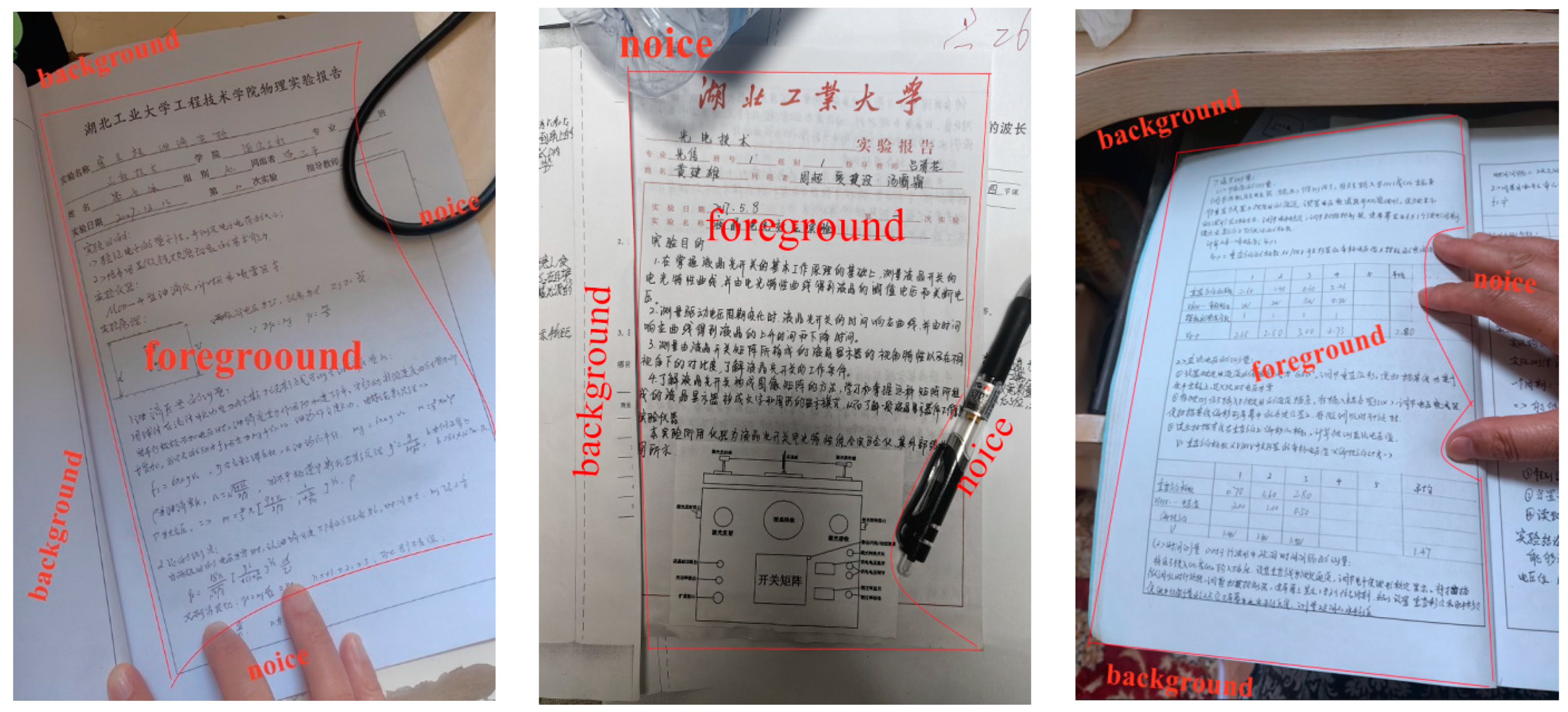
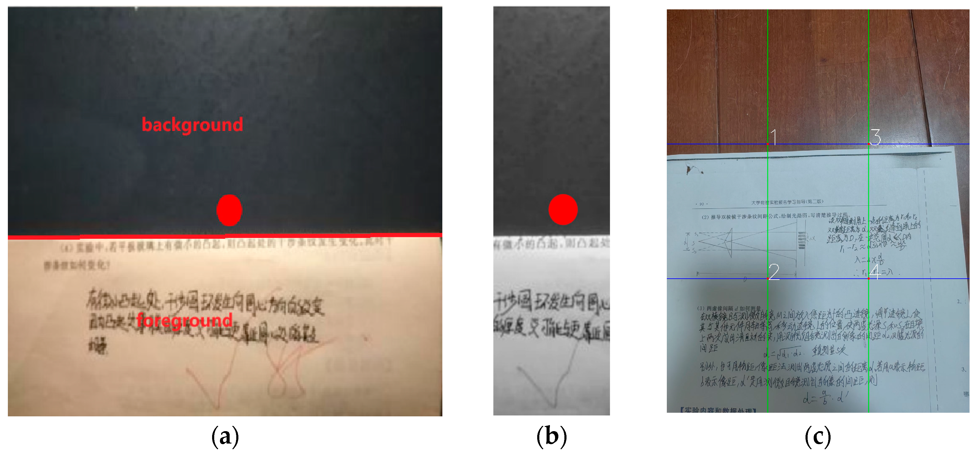
Ineffective segmentation of the foreground across diverse image backgrounds.

(2)

Suboptimal performance when the image center point lies outside the target area.

(3)

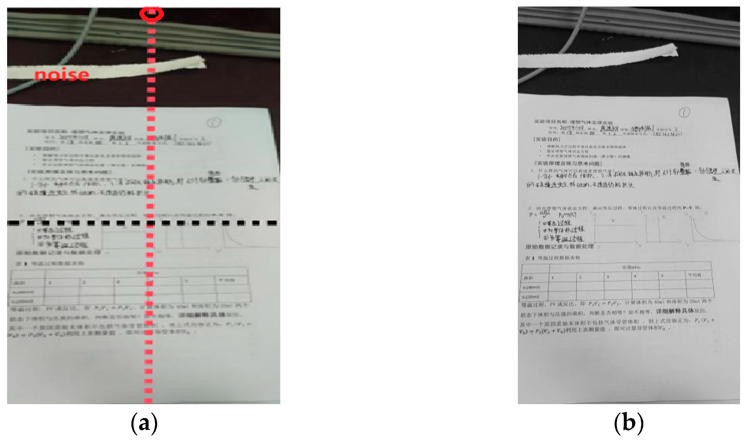
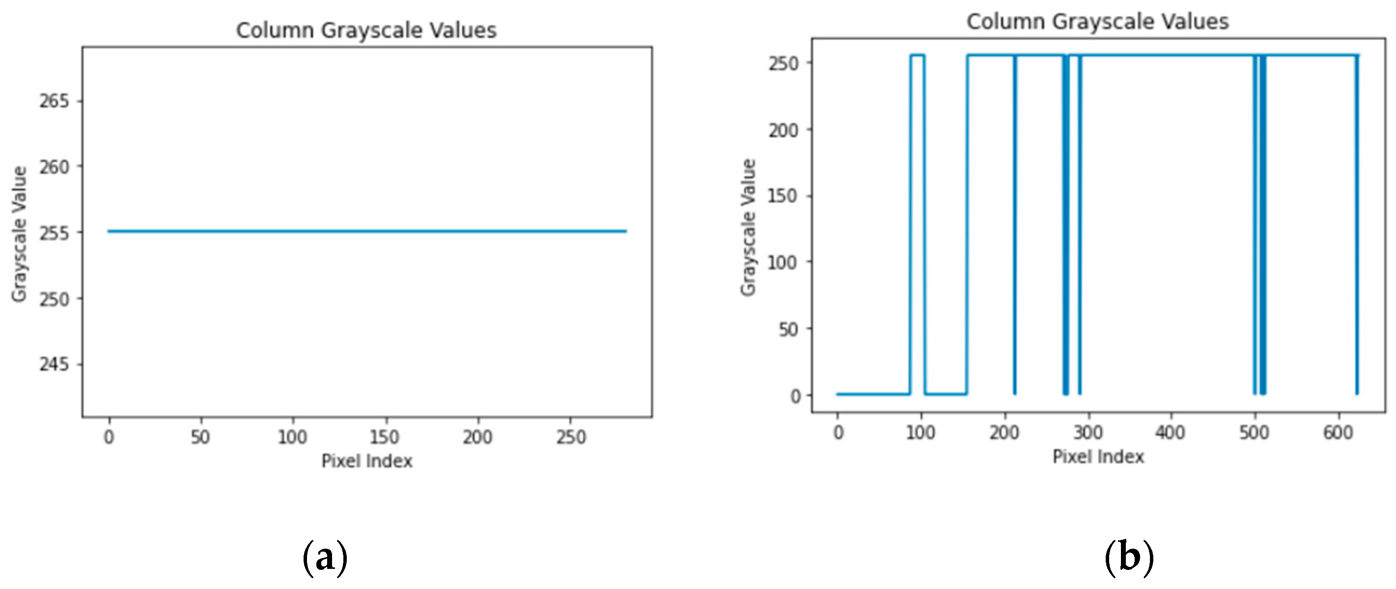
High sensitivity to noise and reduced robustness in determining the start and end points of the segmentation area.

To address these issues, this study proposes the following solutions:

(1)

Dynamic Thresholding for Background Adaptation

The fixed threshold in the Magefreehome algorithm is replaced with a dynamic threshold to improve foreground segmentation across varying image backgrounds. The optimal dynamic threshold is first determined using the OTSU algorithm, which is then applied to binarize the image, allowing for adaptation to different backgrounds and reducing their influence. Additionally, a shadow detection mechanism is introduced to identify shadows; if shadows are detected, the start and end points of the segmentation foreground are reset. This refinement improves precision and recall by 8.00% and 8.42%, respectively, without affecting processing speed.

(2)

Improved Image Center Point Selection

To resolve the issue of suboptimal segmentation performance when the image center falls outside the target area, an improved method for selecting the image center point is proposed. This method calculates multiple reference center points to determine the optimal center point of the image. This enhancement improves precision and recall by 5.17% and 1.18%, respectively, while maintaining the same processing speed.

(3)

Noise-Resilient Start/End Point Determination

To mitigate the sensitivity to noise when determining the start and end points of the segmentation foreground, a method based on continuity detection is proposed. This method leverages the characteristic that pixels within the segmented region generally have similar grayscale values while the region’s boundaries exhibit grayscale discontinuity. It detects the continuity of coordinates with a grayscale value of 255 in rows and columns to identify the presence of noise. If noise is detected, the segment with the highest number of continuous coordinates is selected as the target region, and its endpoints are set as the start and end points of the segmentation foreground. This approach enhances precision and recall by 6.61% and 5.71%, respectively, without impacting processing speed.

The remaining components of the paper are structured as follows: Section 2 discusses related work, Section 3 details the proposed method, Section 4 presents the experimental results, analysis, and significance, and Section 5 concludes the paper.

2. Preliminary

Magfreehome

Image Border Removal refers to the process of eliminating peripheral black regions in an image, retaining only the relevant content to enhance the subject’s prominence and provide a cleaner visual effect. This procedure improves both the image’s aesthetic appeal and usability. Python-based algorithms are commonly used for this task due to their flexibility in detecting and removing edge pixels. However, traditional methods often rely on iterative loops to scan pixel-by-pixel, which can be computationally intensive. This approach reduces efficiency, particularly when processing high-resolution images or large datasets, as it leads to slower performance.

In 2022, a blogger named ‘Magefreehome’ introduced an innovative image segmentation technique that enhances processing speed. The method vectorizes the grayscale values of pixels along the row or column passing through the image’s center and filters pixels based on a predefined threshold. Only pixels exceeding this threshold are retained for further processing, allowing efficient pixel filtering. This algorithm achieves linear time complexity, O(n), making it approximately 100 times faster than conventional techniques. The steps of the algorithm are as follows:

Step 1: Define the threshold.

Step 2: Import the image.

Step 3: Convert the image to grayscale.

Step 4: Retrieve the row and column dimensions of the image.

Step 5: Extract the coordinates of pixels along the central row or column whose grayscale values exceed the threshold.

Step 6: Identify the first and last coordinates of the extracted pixels as segmentation boundaries.

Step 7: Segment the original image based on these boundaries and display the result.

Grayscale value [46] refers to the brightness level of pixels in black-and-white images, ranging from 0 to 255. A higher grayscale value indicates greater pixel brightness, while a lower grayscale value indicates lesser pixel brightness.

The threshold [47] is a critical value used to distinguish different grayscale levels and is typically employed to convert grayscale images into binary images. During threshold processing, all pixels with grayscale values greater than or equal to the threshold are assigned a specific value (usually 255), while pixels with grayscale values less than the threshold are assigned another specific value (usually 0).

NumPy [45] (Numeric Python) is a fundamental library for scientific computing in Python. It provides multidimensional array objects, derived objects, and routines for fast array operations. Its core is the Ndarray object, which encapsulates n-dimensional arrays of homogeneous data types, with many operations executed in compiled code to enhance performance.

The OTUS algorithm [48] is a metaheuristic algorithm used to solve optimization problems. The full name is One-Tenth Up-Hill Search, an improved algorithm based on hill climbing. The basic idea of the OTUS algorithm is to randomly select an initial solution within the solution space and then iteratively search for an optimal solution. In each iteration, the algorithm performs a local search around the current solution and updates it based on the search results. The key lies in choosing the appropriate search direction and step size to quickly find the optimal solution. Compared to traditional optimization algorithms, the OTUS algorithm offers advantages such as simplicity, ease of implementation, and robustness.

3. Methodology

In response to the deficiencies of the Magefreehome algorithm, this study implements the following improvements.

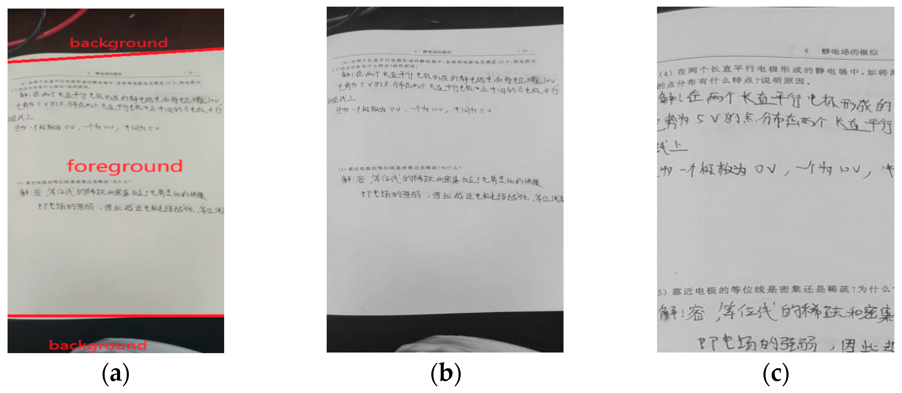
3.1. Improved Scheme Based on OTSU Dynamic Threshold Calculation: Strategy 1

The core of the Magefreehome algorithm lies in segmenting the image by comparing the grayscale values of the pixels in the rows and columns where the image center point is located against a set threshold. This threshold directly determines segmentation accuracy. When the image background varies, the grayscale values of the pixels can differ, making a fixed threshold insufficient for precise segmentation. If the threshold is set too low, background pixels may be included, causing the segmented image to retain irrelevant parts (Figure 2b). Conversely, if the threshold is set too high, many pixels from the target area may be excluded, resulting in the foreground being mistakenly cut off and the loss of valid information (Figure 2c).

This paper proposes an improved scheme based on OTSU dynamic threshold calculation. The OTSU algorithm, which operates on the principle of maximizing inter-class variance, segments the image into foreground and background according to the grayscale distribution characteristics. The objective is to minimize the global brightness difference and the squared difference between the two segments. During the algorithm’s execution, the histogram of the grayscale image is analyzed to automatically calculate the inter-class variance for each potential threshold. The threshold with the maximum inter-class variance is selected as the optimal threshold, enabling the grayscale image to be segmented into foreground and background, accordingly, thereby achieving a dynamically adaptive threshold that adjusts to the image background.

However, the OTSU algorithm for image segmentation is often affected by shadows [49,50,51]. Specifically, when the row or column containing the image center point falls within a deep shadow area (Figure 3a), the grayscale values in these regions may drop to 0 during binarization, causing these points to be ignored in the detection process. This can result in incorrect segmentation of the shadow area, leading to over-segmentation (Figure 3b). To address this issue, a shadow detection mechanism is introduced. Before segmentation, the algorithm first detects the presence of shadows in the image. If shadows are present and the row of the image center point intersects the shadow area, the grayscale values of these points will change relatively gradually, meaning they change slowly with a certain slope (Figure 4a). Conversely, if the column does not intersect the shadow area, the grayscale values of the points will change more significantly. If no shadows are present (Figure 5a), the grayscale values of the points in the row or column containing the center point will exhibit significant jumps (Figure 5b,c), making it easier to distinguish the background from the foreground.

The shadow detection mechanism proposed in this paper operates as follows.

Let $G_n$ represent the grayscale value of the n-th predicted target segmentation point, $G_{n-i}$ represent the grayscale value of the point located $i$ positions before the n-th predicted target segmentation point, and $G_{n+i}$ represent the grayscale value of the point located $i$ positions after the n-th predicted target segmentation point. $G_a$ and $G_b$ denote the average grayscale values, respectively, and are defined as follows:

$$G_a={\displaystyle \frac{{\displaystyle \sum _1^i{G}_{n-i}}}{i}}$$

(1)

$${\mathrm{G}}_b={\displaystyle \frac{{\displaystyle \sum _1^i{G}_{n+i}}}{i}}$$

(2)

Here, $dist.$ refers to the distance between the n-th predicted target segmentation point and the image boundary.

To accurately determine the presence of shadows within an image, this paper proposes Algorithm 1: Shadow Detection and Segmentation. This algorithm systematically implements a conditional judgment mechanism that assesses shadow presence by calculating the distance between the segmentation point and the image boundary, as well as by analyzing the grayscale differences between adjacent points. The algorithm’s detailed logic is outlined in the pseudocode below.

Algorithm 1. Shadow Detection and Segmentation
Input: $dist.$, $G_a$, $G_b$
Output: Shadow and segmentation reset
1:	If $dist.$ < 5,
2:	no shadow
3:	else If $|G_a-G_b|>10$
4:	no shadow
5:	Else
6:	shadow
7:	Resets the segmentation start or end point to the image edge
8:	end

In Algorithm 1, the values 5 and 10 are empirically determined. During the development of the algorithm, various values were tested and adjusted through continuous experimentation, with performance and results observed. It was concluded that, under multicolor backgrounds, static photography, and stable indoor lighting conditions, 5 and 10 are the optimal empirical values.

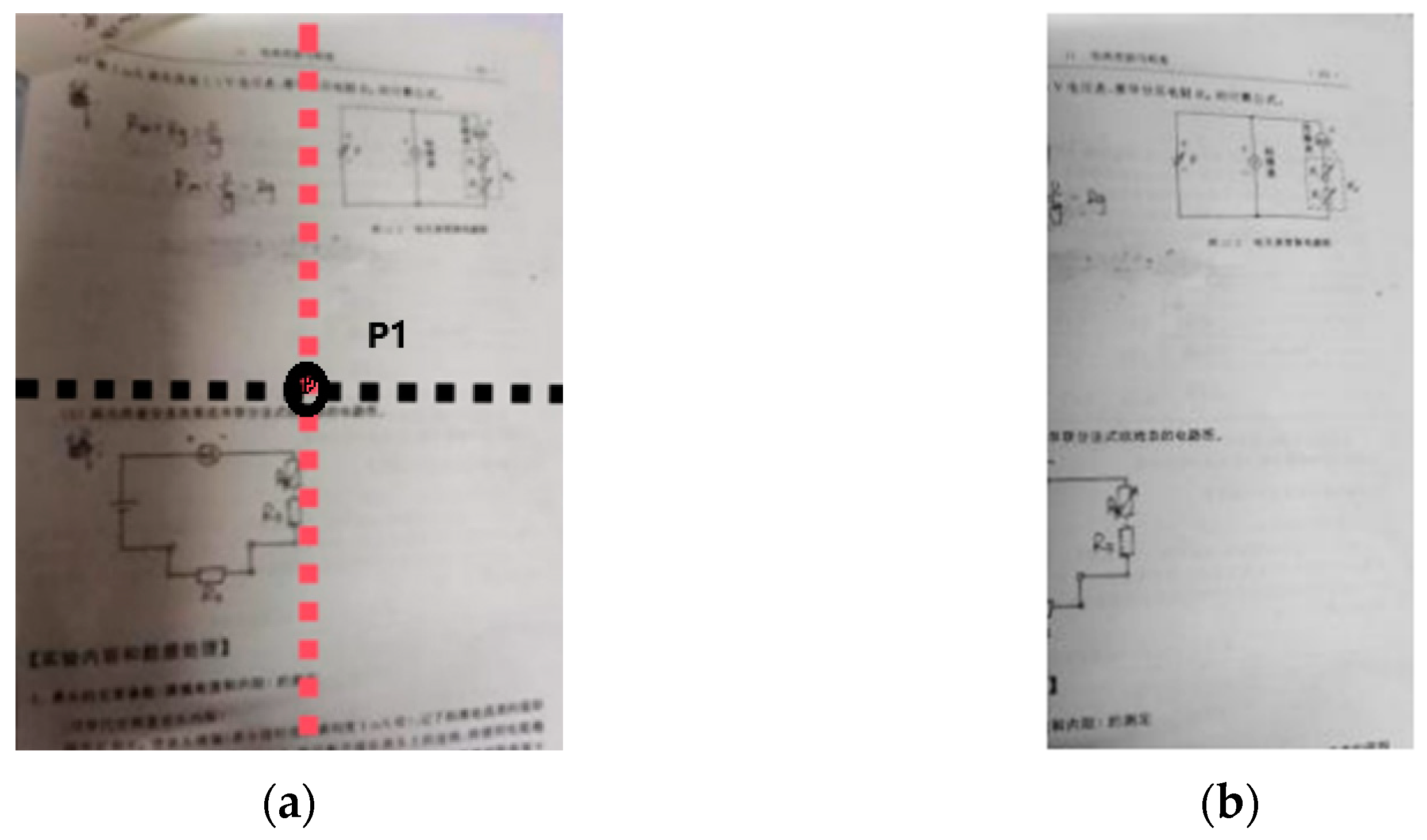
3.2. An Improved Method for Selecting Image Center Points: Strategy 2

The Magefreehome algorithm determines the image center point by calculating the image dimensions. However, if the center point falls outside the segmentation foreground region (Figure 6a), the grayscale values of the pixels in the row or column containing the center point may drop below the set threshold, resulting in excessive cropping of the image (Figure 6b).

Dividing an image into a 3 × 3 grid is a widely used design technique to ensure balance and alignment of image elements. Based on this method, extracting the four intersection points located at the one-third and two-thirds positions of the image’s rows and columns highlights key points in the grid. These points are typically used to identify important visual elements or to facilitate further image-processing tasks. The center points derived from the 3 × 3 grid principle can be utilized in various image processing applications, such as alignment, cropping, and feature extraction. Based on this principle, we propose an improved method for selecting the image center point. Initially, four intersection points at one-third and two-thirds of the image’s rows and columns are taken as reference points (Figure 6c). To reduce computational load, the points along the vertical and horizontal axes of these reference points are sparsified by retaining only one out of every three points. Subsequently, the grayscale values of the points in the rows and columns of these four reference points are calculated. The OTSU algorithm is then employed to compute the dynamic threshold, followed by binarization. Finally, the number of points with a grayscale value of 255 is counted, and the row or column with the highest count is selected as the reference line. The intersection of this row and column is chosen as the center point of the segmentation foreground.

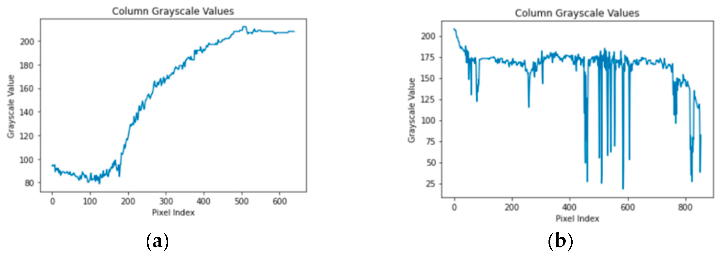
3.3. A Method for Determining the Start/End Points of the Segmentation Region Based on Continuity Detection: Strategy 3

The Magefreehome algorithm is highly sensitive to noise and lacks robustness in determining the segmentation start and end points. When the start or end points fall within noise areas with high grayscale values outside the segmentation foreground region, these noise areas are mistakenly considered part of the segmentation foreground, resulting in incomplete segmentation. In Figure 7a, the start point falls within a noise area, and in Figure 7b, the segmented image still contains these noise areas.

We propose a continuity detection-based method for determining the segmentation start and end points. This method detects the continuity of coordinates with a grayscale value of 255 in the row or column where the image center point is located to identify the presence of noise. In the segmentation foreground region, the coordinates of points with a grayscale value of 255 are generally continuous without jumps (Figure 8a), whereas noise causes abrupt changes that disrupt continuity (Figure 8b). Therefore, we stipulate that if the distance between points with a grayscale value of 255 does not exceed one-tenth of the total row or column length, the coordinates are considered continuous and noise-free. In this case, we select the segment with the most such points as the target segmentation foreground region, with its two endpoints determined as the start and endpoints of the segmentation.

3.4. Fully Automatic Grayscale Image Segmentation Algorithm

To address the deficiencies of the Magefreehome algorithm in image segmentation, we propose three strategies for improvement and introduce the Fully Automatic Grayscale Image Segmentation Algorithm. The process is as follows:

Step 1: Read the image to be segmented and convert it to grayscale.

Step 2: Apply the improved OTSU algorithm (Strategy 1) to find the optimal threshold and perform binarization.

Step 3: Implement the improved method for selecting the image center point (Strategy 2) to determine the optimal center point.

Step 4: Use the continuity detection-based method to identify the segmentation start and end points (Strategy 3), reducing noise interference.

Step 5: Introduce a shadow detection mechanism (Strategy 1) to reset the segmentation start and end points for images with shadows.

Step 6: Save and output the segmented image.

4. Experiments

4.1. Dataset, Testing Environment and Testing Plan

To validate the effectiveness of the proposed algorithm, it was applied to the physics experiment system of the Hubei University of Technology (wlsy-main (wjygrit.cn)). The experimental dataset was sourced from 203,495 experiment reports uploaded to this system during the 2022–2023 academic year, from which 100,299 images were randomly selected. The images were captured indoors using mobile phones, tablets, etc., either from an overhead or horizontal perspective. The lighting conditions were stable, with moderate intensity. Due to side lighting, more than 95% of the images exhibit varying levels of shadow. The shooting environments were complex, featuring multi-colored backgrounds, and in addition to the primary subjects, the images contained extraneous elements such as furniture, appliances, decorations, and stationery. Approximately 2% of the images contain Gaussian noise, which results in blurred object contours and textures. The images are in JPEG format, with file sizes ranging from 100 KB to 400 KB.

The algorithm was developed and executed using OpenCV (version 4.6.0) on a Windows operating system with hardware specifications including an 11th Gen Intel(R) Core (TM) i5-1135G7 @ 2.40GHz CPU. The performance of the Magefreehome algorithm was compared with the proposed algorithm in terms of effectiveness, performance, and the impact of different strategies.

Initially, these images were processed using the Magefreehome algorithm, resulting in 15,064 images with suboptimal results. The deficiencies were categorized as follows:

(1)

Incomplete or excessive segmentation due to fixed thresholds (10,436 images, 69.28%);

(2)

Segmentation errors caused by improper selection of the image center point (3905 images, 25.92%);

(3)

Incomplete segmentation due to weak anti-interference capabilities (723 images, 4.80%).

4.2. Comparison of Image Segmentation Effectiveness

To evaluate the effectiveness of the proposed algorithm, the three improvement strategies were applied to address each type of defect respectively. By visually comparing the images processed by the original and proposed algorithms, we assessed the effectiveness of image segmentation.

4.2.1. Effectiveness of the Improved OTSU Dynamic Threshold Calculation Strategy

Segmentation was performed on 21,520 images with fixed threshold issues, with representative results shown below.

The original algorithm’s fixed threshold approach resulted in incomplete segmentation (Figure 9b) or excessive segmentation (Figure 10a) due to background differences. In contrast, the proposed OTSU-based method dynamically calculates the optimal threshold based on the grayscale distribution, minimizing global brightness differences and achieving precise segmentation (Figure 10b).

To address shadow interference in the OTSU algorithm, which results in over-segmentation by disregarding shadow regions (Figure 11b and Figure 12a), we introduced a shadow detection mechanism. By resetting the segmentation points to the image edges upon shadow detection, the proposed method achieved optimal segmentation results (Figure 12b), effectively mitigating shadow interference.

4.2.2. Effectiveness of the Improved Image Center Point Selection Method

When processing 8052 images, the original algorithm, which determined the center point based on image dimensions, led to excessive segmentation (Figure 13b) when the center point was located outside the foreground region (Figure 13a). To address this, the proposed method introduces multiple reference center points, binarizes them based on grayscale values, and identifies the intersection with the highest number of points having a grayscale value of 255 as the foreground center. This approach enables precise segmentation (Figure 13c).

4.2.3. Effectiveness of the Continuity Detection-Based Segmentation Start/End Point Determination Method

During the segmentation of 1491 noisy images (Figure 14a), the original algorithm erroneously included noise in the foreground region, leading to suboptimal performance (Figure 14b). The proposed continuity detection method redefines the segmentation start and end points, effectively excluding noise from the foreground region and achieving complete segmentation (Figure 14c).

4.3. Comparison of Algorithm Performance

To verify the performance of the proposed algorithm, four datasets of varying scales (438, 2098, 6370, and 20,014 images) were randomly selected from a total of 100,299 images. The proposed algorithm was applied to these datasets to comprehensively evaluate their statistical characteristics, generalization ability, and stability. Metrics such as precision, accuracy, recall, and speed were defined and compared with those of the original algorithm.

4.3.1. Performance Metrics

• False Negative (FN): The number of images incorrectly identified by the algorithm as not requiring segmentation, despite actually needing it;
• True Negative (TN): The number of images correctly identified by the algorithm as not requiring segmentation;
• True Positive (TP): The number of images correctly identified by the algorithm as requiring segmentation;
• False Positive (FP): The number of images incorrectly identified by the algorithm as requiring segmentation, despite not needing it.

$$Accuracy={\displaystyle \frac{TP+TN}{TP+TN+FP+FN}}$$

(3)

$$Precision={\displaystyle \frac{TP}{TP+FP}}\mathrm{o}\mathrm{r}Precision={\displaystyle \frac{TN}{TN+FN}}$$

(4)

$$Recall={\displaystyle \frac{TP}{TP+FN}}\mathrm{o}\mathrm{r}Recall={\displaystyle \frac{TN}{TN+FP}}$$

(5)

$$PrecessingSpeed={\displaystyle \frac{TotalnumberofImage}{Totalprocessingtime}}$$

(6)

4.3.2. Experimental Results and Analysis

The

Table 1. The comparisons of algorithm performance after running on varying numbers of images.

Number of Image	Magefreehome				Our Algorithm
	Speed (Number/s)	Accuracy	Precision	Recall	Speed (Number/s)	Accuracy	Precision	Recall
423	48.6	77.17%	99.10%	69.18%	48.34	88.58%	96.40%	83.59%
2098	48.43	74.74%	98.76%	68.30%	47.56	90.94%	98.05%	86.79%
6370	47.54	74.61%	96.66%	66.75%	47.09	91.35%	97.77%	86.46%
20014	32.14	78.32%	97.69%	74.76%	31.38	93.83%	98.71%	91.48%

shows that the overall performance of the proposed algorithm surpasses that of the original algorithm.

(1)

Accuracy: The proposed algorithm achieved a maximum accuracy of 93.83%, representing an improvement of 15.51% over the original algorithm, with an average increase of 14.97%. This success can be attributed to three key factors: the dynamic threshold calculation method, based on the improved OTSU algorithm, enables the algorithm to adaptively adjust the threshold according to varying image backgrounds, leading to enhanced segmentation; the continuity detection method precisely identifies the start and end points of the foreground, effectively excluding impurities and other interference factors; and the improved image center point selection method, which utilizes a multi-center point strategy, makes the algorithm more resilient to noise variations in complex background images.

(2)

Precision: The proposed algorithm achieved a maximum precision of 98.71%, reflecting an increase of only 1.02% over the original algorithm. This modest improvement is attributed to the algorithm’s heightened sensitivity to noise and impurities, despite maintaining high accuracy. The lowest precision, recorded at 96.40%, represents a 2.70% decrease compared to the original algorithm, which was due to occasional misjudgments when processing specific types of images.

(3)

Recall: The proposed algorithm achieved a maximum recall rate of 91.48%, representing an improvement of 16.72% over the original algorithm, with an average increase of 17.33%. This significant improvement is primarily attributed to the continuity detection-based method for determining the segmentation start and end points, which effectively excludes impurities and interference.

(4)

Processing Speed: The proposed algorithm’s processing speed was slightly reduced by 0.585 images per second, approximately 1.34%. However, considering the significant improvements in precision and recall rates, this minor decrease in processing speed is a worthwhile trade-off.

4.4. Ablation Experiment

During the experiments, 20,014 images were randomly selected, and three strategies were integrated into the original algorithm to compare precision, accuracy, recall, and processing speed. The experimental results are presented in

Table 2. Comparison of the Enhancement Degree of the Three Strategies in this Study’s Algorithm.

Algorithm Combination	Speed (Number/s)	Accuracy	Precision	Recall
Magefreehome	32.14	78.32%	97.69%	74.76%
Magefreehome + Strategy1	32.09	86.32%	92.31%	82.05%
Magefreehome + Strategy2	33.44	83.49%	97.12%	75.94%
Magefreehome + Strategy3	31.73	84.93%	99.04%	80.47%
Magefreehome + Strategy1 + Strategy2	32.41	86.76%	94.23%	85.96%
Magefreehome + Strategy1 + Strategy3	32.75	89.04%	96.15%	88.50%
Magefreehome + Strategy2 + Strategy3	32.55	84.02%	98.05%	79.69%
Magefreehome + Strategy1 + Strategy2 + Strategy3	31.38	93.83%	98.71%	91.48%

.

(1)

Single Strategy Usage

Strategy 1: By dynamically adjusting the threshold, the algorithm became more precise in distinguishing the foreground from the background, significantly reducing false negatives and enhancing precision and recall rates by 8.00% and 7.29%, respectively. Although accuracy slightly decreased, the overall performance improved significantly. Strategy 2: The center point selection method was optimized, making the algorithm more accurate and comprehensive in locating the foreground. This resulted in a 5.17% improvement in precision and a 1.18% improvement in recall, with a slight 0.57% decrease in accuracy. Strategy 3: Continuity detection was implemented, enabling the algorithm to more accurately determine the start and end points of the foreground region, thereby increasing target recognition accuracy and reducing false negatives. This strategy improved precision by 6.61%, accuracy by 1.35%, and recall by 5.71%. Overall, the average improvements in precision and recall were 6.59% and 4.73%, respectively, despite a slight 1.53% decrease in accuracy. These optimizations provided strong support for enhancing target detection accuracy and efficiency without affecting processing speed.

(2)

Combination of Two Strategies

Strategies 1 and 2: When combined during image segmentation, these strategies improved precision by 8.44%, demonstrating that dynamic thresholds more accurately identified image content, while the optimized center point selection enhanced segmentation precision. Although minor misjudgments slightly reduced accuracy, recall significantly increased by 11.20%, indicating the algorithm’s enhanced capability in identifying correct segmentation areas. Strategies 1 and 3: This powerful combination further improved precision by 10.72%. The introduction of Strategy 3 enhanced the algorithm’s ability to recognize continuous regions, significantly increasing segmentation precision and recall by 13.74%, reflecting substantial progress in correctly identifying foregrounds. Strategies 2 and 3: The complementary effects of these strategies improved precision by 5.70%, showing that the optimized center point selection method and continuity detection worked synergistically to enhance algorithm performance. A slight increase in accuracy indicated positive contributions in reducing misjudgments, while improvements in recall suggested better recognition of correct segmentation foregrounds. Overall, combining the two strategies resulted in average improvements of 8.29% in precision and 9.96% in recall, indicating more precise differentiation between target and background, reducing false negatives, and improving detection completeness. Despite a slight 1.55% decrease in accuracy, this was acceptable given the overall performance improvement, along with a slight increase in processing speed.

(3)

Combination of All Three Strategies

When the original algorithm combined all three strategies, precision increased by 15.51%, demonstrating the synergistic effect of these strategies in image segmentation. Accuracy also improved, indicating reduced mis-segmentation while maintaining high precision. The recall rate increased by 16.72%, further confirming the enhanced recognition and segmentation capabilities of the algorithm.

Notably, whether a single strategy is employed, two strategies are combined, or all three strategies are utilized together, experiments on image sample sets of varying scales consistently indicate that the processing speed of the proposed algorithm fluctuates by approximately one image per second, either faster or slower, compared to the Magefreehome algorithm. Given the substantial improvements in other performance metrics, this slight variation in processing speed is considered acceptable.

5. Conclusions

With the widespread application of network technology for uploading images, the demand for image segmentation is growing. This paper addresses the limitations of the Magefreehome algorithm in fine segmentation under complex backgrounds and proposes a series of effective improvements based on in-depth analysis and experimental validation. These improvements include the introduction of a dynamic threshold mechanism, enabling the algorithm to automatically adjust thresholds in response to background variations under different lighting and color conditions, significantly enhancing adaptability. The implementation of a shadow detection mechanism effectively mitigates shadow interference in target detection, further improving accuracy. Additionally, the optimization of the image center point selection strategy ensures more accurate localization of the foreground region during processing, enhancing stability. To address sensitivity to noise and limited robustness, a continuity detection-based method for determining segmentation start and end points was developed, improving the algorithm’s generalization ability. These strategies not only preserved the original processing speed but also significantly enhanced accuracy and recall rates, resulting in outstanding performance in segmentation tasks under complex backgrounds. In the future, integrating deep learning techniques could further optimize the adaptability of dynamic thresholds with image backgrounds, explore methods to improve precision, and refine the handling of shadows and noise, thereby bolstering the algorithm’s robustness and enabling more precise and efficient image segmentation. Besides these, the OTSU algorithm can struggle with more complex grayscale images, where histograms might not have clear bimodal distributions, which is not included in the algorithm of this paper, and we will further study in the future.

References

- Image Processing Procedure. Available online: https://blog.csdn.net/sinat_31608641/article/details/102789221 (accessed on 27 February 2023).
- Rafique, A.A.; Gochoo, M.; Jala, A.; Kim, K. Maximum entropy scaled super pixels segmentation for multi-object detection and scene recognition via deep belief network. Multimed. Tools Appl. 2023, 80, 13401–13430. [Google Scholar] [CrossRef]
- Huang, L.; Ruan, S.; Denoeux, T. Application of belief functions to medical image segmentation: A review. Inform. Fusion 2023, 91, 737–756. [Google Scholar] [CrossRef]
- Cao, W.W.; Yuan, G.; Liu, Q.; Peng, C.T.; Xie, J.; Yang, X.D.; Ni, X.Y.; Zheng, J. ICL-Net: Global and local inter-pixel correlations learning network for skin lesion segmentation. IEEE J. Biomed. Health Inform. 2022, 27, 145–156. [Google Scholar] [CrossRef] [PubMed]
- Dang, T.V.; Bui, N.T. Multi-scale fully convolutional network-based semantic segmentation for mobile robot navigation. Electronics 2023, 12, 533. [Google Scholar] [CrossRef]
- Yu, J.; Zhang, J.; Shu, Y.; Chen, Y.; Chen, J.; Yang, Y.; Tang, W.; Zhang, Y. Study of convolutional neural network-based semantic segmentation methods on edge intelligence devices for field agricultural robot navigation line extraction. Comput. Electron. Agric. 2023, 209, 107811. [Google Scholar] [CrossRef]
- Schein, K.E.; Marc, H.; Rauschnabel, P.A. How do tourists evaluate augmented reality services? Segmentation, awareness, devices and marketing use cases. In Springer Handbook of Augmented Reality; Springer International Publishing: Cham, Switzerland, 2023; pp. 451–469. [Google Scholar]
- Klingenberg, S.; Fischer, R.; Zettler, I.; Makransky, G. Facilitating learning in immersive virtual reality: Segmentation, summarizing, both or none? J. Comput. Assist. Learn. 2023, 39, 218–230. [Google Scholar] [CrossRef]
- Min, H.; Zhang, Y.M.; Zhao, Y.; Zhao, Y.; Jia, W.; Lei, Y.; Fan, C. Hybrid feature enhancement network for few-shot semantic segmentation. Pattern Recognit. 2023, 137, 109291. [Google Scholar] [CrossRef]
- Tummala, S.K. Morphological operations and histogram analysis of SEM images using Python. Indian J. Eng. Mater. Sci. 2023, 29, 796–800. [Google Scholar]
- Lin, X.F.; Li, C.J.; Adams, S.; Kouzani, A.Z.; Jiang, R.; He, L.G.; Hu, Y.J.; Vernon, M.; Doeven, E.; Webb, L.; et al. Self-supervised leaf segmentation under complex lighting conditions. Pattern Recognit. 2023, 135, 109021. [Google Scholar] [CrossRef]
- Bagwari, N.; Kumar, S.; Verma, V.S. A comprehensive review on segmentation techniques for satellite images. Arch. Comput. Methods Eng. 2023, 30, 4325–4358. [Google Scholar] [CrossRef]
- Physics Experiment Management System of Hubei University of Technology. Available online: https://wlsy.wjygrit.cn/login (accessed on 12 October 2023).
- Yu, Y.; Wang, C.P.; Fu, Q.; Kou, R.; Huang, F.; Yang, B.; Yang, T.; Gao, M. Techniques and challenges of image segmentation: A review. Electronics 2023, 12, 1199. [Google Scholar] [CrossRef]
- Gopalakrishnan, C.; Iyapparaja, M. Multilevel thresholding based follicle detection and classification of polycystic ovary syndrome from the ultrasound images using machine learning. Int. J. Syst. Assur. Eng. Manag. 2021, 1–8. [Google Scholar] [CrossRef]
- Du, J.L.; Zhang, Y.Q.; Jin, X.Y.; Zhang, X. A cell image segmentation method based on edge feature residual fusion. Methods 2023, 219, 111–118. [Google Scholar] [CrossRef] [PubMed]
- Zhang, X.Y.; Han, X.; Fu, C.N. Comparison of Object Region Segmentation Algorithms of PCB Defect Detection. Trait. Signal 2023, 40, 797–802. [Google Scholar] [CrossRef]
- Fang, K. Threshold segmentation of PCB defect image grid based on finite difference dispersion for providing accuracy in the IoT based data of smart cities. Int. J. Syst. Assur. Eng. Manag. 2022, 13, 121–131. [Google Scholar] [CrossRef]
- Khairnar, S.; Thepade, S.D.; Gite, S. Effect of image binarization thresholds on breast cancer identification in mammography images using OTSU, Niblack, Burnsen, Thepade’s SBTC. Intell. Syst. Appl. 2021, 10, 200046. [Google Scholar] [CrossRef]
- Abualigah, L.; Khaled, H.; Almotairi, K.H.; Elaziz, M.A. Multilevel thresholding image segmentation using meta-heuristic optimization algorithms: Comparative analysis, open challenges and new trends. Appl. Intell. 2023, 53, 11654–11704. [Google Scholar] [CrossRef]
- Sasmal, B.; Dhal, K.G. A survey on the utilization of Superpixel image for clustering based image segmentation. Multimed. Tools Appl. 2023, 82, 35493–35555. [Google Scholar] [CrossRef]
- Luo, Z.F.; Yang, Y.W.; Gou, Y.R.; Li, X. Semantic segmentation of agricultural images: A survey. Inf. Process. Agric. 2023, 11, 172–186. [Google Scholar] [CrossRef]
- Amiriebrahimabadi, M.; Zhina, R.; Najme, M. A Comprehensive Survey of Multi-Level Thresholding Segmentation Methods for Image Processing. Arch. Comput. Methods Eng. 2024, 31, 1–51. [Google Scholar] [CrossRef]
- Miao, T.; Zhen, H.C.; Wang, H.; Chen, J. Rapid extraction of spaceborne SAR flood area based on iterative threshold segmentation. Syst. Eng. Electron 2022, 44, 2760–2768. [Google Scholar]
- Lang, J.W.; Bai, F.Z.; Wang, J.X.; Gu, N.T. Progress on region segmentation techniques for optical interferogram. Opt. Instrum. 2023, 45, 87–94. [Google Scholar]
- Ingh, N.S.; Bhandari, A.K. Multiclass variance based variational decomposition system for image segmentation. Multimed. Tools Appl. 2023, 82, 41609–41639. [Google Scholar]
- Hosny, K.M.; Khalid, A.M.; Hamza, H.M.; Mirjalili, S. Multilevel thresholding satellite image segmentation using chaotic coronavirus optimization algorithm with hybrid fitness function. Neural Comput. Appli. 2023, 35, 855–886. [Google Scholar] [CrossRef]
- Abualigah, L.; Al-Okbi, N.K.; Elaziz, M.A.; Houssein, E.H. Boosting Marine Predators Algorithm by Salp Swarm Algorithm for Multilevel Thresholding Image Segmentation. Multimed. Tools Appl. 2022, 81, 16707–16742. [Google Scholar] [CrossRef]
- Abdel-Basse, M.; Mohamed, R.; Abouhawwash, M. A new fusion of whale optimizer algorithm with Kapur’s entropy for multi-threshold image segmentation: Analysis and validations. Artif. Intel. Rev. 2022, 55, 6389–6459. [Google Scholar] [CrossRef]
- Zou, Y.B.; Zhang, J.Y.; Zhou, H.; Sun, F.S.; Xia, P. Tsallis Entropy Thresholding Based on Multi-scale and Multi-direction Gabor Transform. J. Electron. Inf. Technol. 2023, 45, 707–717. [Google Scholar]
- Naik, M.K.; Panda, R.; Abraham, A. An entropy minimization based multilevel colour thresholding technique for analysis of breast thermograms using equilibrium slime mould algorithm. Appl. Soft Comput. 2021, 113, 107955. [Google Scholar] [CrossRef]
- Abdel-Khalek, S.; Ishak, A.B.; Omer, O.A.; Obada, A.S.H.F. A two-dimensional image segmentation method based on genetic algorithm and entropy. Optik 2017, 131, 414–422. [Google Scholar] [CrossRef]
- Shubham, S.; Bhandari, A.K. A generalized Masi entropy based efficient multilevel thresholding method for color image segmentation. Multimed. Tools Appl. 2019, 78, 17197–17238. [Google Scholar] [CrossRef]
- Ray, S.; Parai, S.; Das, A.; Dhal, K.G.; Naskar, P.K. Cuckoo search with differential evolution mutation and Masi entropy for multi-level image segmentation. Multimed. Tools and Appl. 2022, 81, 4073–4117. [Google Scholar] [CrossRef]
- Li, H.B.; Zheng, G.; Sun, K.J.; Jang, Z.C.; Yao, L.; Jia, H.M. A logistic chaotic barnacles mating optimizer with Masi entropy for color image multilevel thresholding segmentation. IEEE Access 2020, 8, 213130–213153. [Google Scholar] [CrossRef]
- Li, H.; Peng, S. Image-Based Fire Detection Using Dynamic Threshold Grayscale Segmentation and Residual Network Transfer Learning. Mathematics 2023, 11, 3940. [Google Scholar] [CrossRef]
- Salvi, M.; Acharya, U.R.; Molinari, F.; Meiburger, K.M. The impact of pre-and post-image processing techniques on deep learning frameworks: A comprehensive review for digital pathology image analysis. Comput. Biol. Med. 2021, 128, 104129. [Google Scholar] [CrossRef] [PubMed]
- Kirichev, M.; Slavov, T.; Momcheva, G. Fuzzy U-net neural network design for image segmentation. In The International Symposium on Bioinformatics and Biomedicine; Springer International Publishing: Cham, Switzerland, 2020; Volume 374, pp. 177–184. [Google Scholar]
- Ge, Y.F.; Zhang, Q.; Sun, Y.T.; Shen, Y.D.; Wang, X.Y. Grayscale medical image segmentation method based on 2D&3D object detection with deep learning. BMC Med. Imaging 2022, 22, 33. [Google Scholar]
- Srivastava, V.; Gupta, S.; Singh, R.; Gautam, V.K. A multi-level closing based segmentation framework for dermatoscopic images using ensemble deep network. Int. J. Syst. Assur. Eng. Manag. 2024, 15, 3926–3939. [Google Scholar] [CrossRef]
- Venugopal, V.; Joseph, J.; Das, M.V.; Nath, M.K. DTP-Net: A convolutional neural network model to predict threshold for localizing the lesions on dermatological macro-images. Comput. Biol. Med. 2022, 148, 105852. [Google Scholar] [CrossRef] [PubMed]
- Chen, Y.; Zhou, Y.; Tran, S.; Park, M.; Hadley, S.M. Lacharite and Q. Bai, A self-learning approach for beggiatoa coverage estimation in aquaculture. In Australasian Joint Conference on Artificial Intelligence; Springer International Publishing: Cham, Switzerland, 2022; pp. 405–416. [Google Scholar]
- Ramesh Babu, P.; Srikrishna, A.; Gera, V.R. Diagnosis of tomato leaf disease using OTSU multi-threshold image segmentation-based chimp optimization algorithm and LeNet-5 classifier. J. Plant Dis. Prot. 2024, 1–16. [Google Scholar] [CrossRef]
- Python OpenCV Image Black Trimming. Available online: https://blog.csdn.net/magefreehome/article/details/125307141?spm=1001.2014.3001.5502 (accessed on 15 June 2022).
- Harris, C.R.; Millman, K.J.; Van Der Walt, S.J.; Gommers, R.; Virtanen, P.; Cournapeau, D.; Wieser, E.; Taylor, J.; Berg, S.; Smith, N.J.; et al. Array programming with NumPy. Nature 2020, 585, 357–362. [Google Scholar] [CrossRef]
- Gray Value Summary. Available online: https://blog.csdn.net/Tony_Stark_Wang/article/details/79953180 (accessed on 15 April 2018).
- Threshold Based Segmentation Method. Available online: https://blog.csdn.net/weixin_44686138/article/details/130189165 (accessed on 27 September 2023).
- Otsu, N. A threshold selection method from gray-level histograms. IEEE Trans. Syst. Man Cybern. 1979, 9, 62–66. [Google Scholar] [CrossRef]
- Chen, L.P.; Gao, J.H.; Lopes, A.M.; Zhang, Z.Q.; Chu, Z.B.; Wu, R.C. Adaptive fractional-order genetic-particle swarm optimization Otsu algorithm for image segmentation. Appl. Intell. 2023, 53, 26949–26966. [Google Scholar] [CrossRef]
- Gong, J.; Li, L.Y.; Chen, W.N. Fast recursive algorithms for two-dimensional thresholding. Pattern Recognit. 1998, 31, 295–300. [Google Scholar] [CrossRef]
- Sahoo, P.K.; Arora, G. A thresholding method based on two-dimensional Renyi’s entropy. Pattern Recognit. 2004, 37, 1149–1161. [Google Scholar] [CrossRef]