Abstract
Every part of society relies on energy systems due to the growing population and the constant demand for energy. Because of the high energy demands of transportation, industry, and daily life, energy systems are crucial to every part of society. Electrical transmission lines are a crucial component of the electrical power system. Therefore, in order to determine the power system’s protection plan and increase its reliability, it is critical to foresee and classify fault types. With this motivation, the main goal of this paper is to design a deep network model to classify faults in transmission lines based on real, generated, and publicly available datasets. A deep learning architecture that was based on a one-dimensional convolutional neural network (CNN) was utilized in this study. Accuracy, specificity, recall, precision, F1 score, ROC curves, and AUC were employed as performance criteria for the suggested model. Not only synthetic but also real data were used in this study. It has been seen that the created model can be used successfully for both real data and synthetic data. In order to measure the robustness of the network, it was tested with three different datasets consisting of real, generated, and publicly available datasets. In the paper, 1D CNN, one of the machine learning methods, was used on three different power systems, and it was observed that the machine learning method was successful in all three power systems.
1. Introduction
The necessity for energy and the growing population have made energy systems crucial to every aspect of society. Energy systems are essential to all facets of society because of the demand for energy, particularly in the areas of transportation, industry, and home life. An essential part of the electrical power system is the electric transmission lines. Consequently, in order to create the power system’s protection strategy and increase its dependability, it is essential to anticipate and identify the kinds and locations of faults. This increases the entire power system’s efficiency and dependability by cutting down on the amount of time needed for a particularly lengthy transmission line. Generally speaking, transmission line protection systems operate by identifying the fault and isolating just the affected area [1,2]. To improve the dependability of power systems, inspections are performed on the electrical system’s component parts. The demand for smart grid protection, control, and monitoring increases with distributed energy generation. The electrical grid is now much more reliable and adaptable as a result of the widespread use of smart gadgets. In power systems, placement, classification, and fault detection are essential to ensure that any problems are resolved immediately and that the smart network is restarted as quickly as possible. Due to the limitations of kinetic energy storage and the dynamic response of electronic power converters in distributed power systems, the microgrid is in need of fast and adaptive fault classification procedures [3]. Transmission line fault detection and classification is very important for fault root cause analysis and rapid recovery of the power system [4].
Deep learning techniques offer significant advantages since they can automatically extract representative features from vast datasets for fault analysis [5]. Enhancing the power transmission system’s protective protocols can be achieved through the application of strong machine learning algorithms for fault prediction. Artificial intelligence-based models and algorithms are becoming more and more widespread and essential for expediting processes and optimizing strategies for meeting rising energy demand. Machine learning continues to become one of the most important drivers of smart electrical power systems [6]. The aforementioned illustrates the increasing enthusiasm and swift growth surrounding the application of machine learning methodologies to effectively tackle the multifaceted technological obstacles associated with the smart grid [7]. Artificial intelligence plays an important role in power system problems such as operation, protection, control, planning, and diagnosis. Looking through the literature, we can see that research on finding transmission line defects has started. Deep learning techniques are frequently used to classify fault conditions in transmission lines [8]. Presently available deep learning-based fault detection techniques necessitate the collection of substantial volumes of data under various fault scenarios [9]. These methods are being used in a study that addresses the fault scenario that arises from missing parts in insulator chains [10].
Future sustainable energy systems have had their level of resilience assessed through the use of machine learning-based approaches and methods for quantifying energy system resilience [11]. A study was performed investigate the potential role of artificial intelligence in electrical system fault diagnosis operation and to review and analyze the existing research literature in this field [12]. Nominal operation and fault voltage and current data of two different transmission lines and ten different fault types were created with MATLAB Simulink, and sudden fault detection and classification studies were carried out with machine learning methods [13]. A study was conducted on the classification of faults in power systems using three models and machine learning methods together with artificial neural networks [14]. By combining real-time, cutting-edge fault detection sensors created by the Technical University of Ostrava with machine learning models, it provides an automated fault detection method that addresses the drawbacks of traditional fault detection techniques [15]. To increase the capabilities of intelligent methods and avoid dependence on large amounts of labeled data, a new fault identification method based on deep reinforcement learning (DRL) is being investigated in the field of fault identification [16]. An alternate method for classifying transmission line faults makes use of deep learning techniques, with an emphasis on the investigation of five different kinds of short-circuit faults in power systems [17]. Using fault detection and classification techniques, Radu-Adrian and Maria Cristea were able to increase transmission system efficiency and prevent significant damage [18].
It becomes clear from examining the papers that fault detection and classification are the main research topics. Some of the research using machine learning techniques is presented in Table 1.

Table 1.
A few studies using machine learning techniques for fault identification and classification.
The rest of this paper is organized as follows. Section 2 introduces the real experimental and simulation data employed in this study, the proposed deep learning model design of the associated neural network model, and the establishment of parameters and assessment criteria. Section 3 describes the experimental results and the analysis of the results. Section 4 concludes the paper.
2. Material and Methods
2.1. Datasets
In the literature, datasets can be generated synthetically for offline training of models. Frequently, datasets are generated from simulated power systems rather than using real data from the field. For instance, through the utilization of simulation, it is possible to acquire a dataset that encompasses 10 distinct categories of short-circuit fault classes, namely AB, AC, BC, ABG, ACG, BCG, AG, BG, CG, and ABC. As illustrated in Figure 1, these faults are categorized as line to ground (LG), line to line (LL), line to line to ground faults (LLG), and line to line to line faults (LLL). Of these, only the LLL fault is symmetrical, while the other faults are asymmetrical [21]. In this study, one fault from each group was evaluated, and the faults evaluated are shown as red boxes in Figure 1.

Figure 1.
Short-circuit fault type classification. Where A, B, C, and G stand for phase A, phase B, phase C, and ground, respectively.
Three different datasets were used to determine the performance of the proposed model. These models include the following: (a) the real dataset obtained from Gediz Elektrik Company [26], (b) the public dataset [27], and (c) the dataset obtained by creating the Simulink model. In all three datasets, four different transmission line faults were evaluated as shown in the Table 2.

Table 2.
Different types of faults in datasets.
- (a)
- Dataset 1: Real (Gediz) dataset
Real-time data were obtained from the Gediz Elektrik Company. Since 2013, it has been providing 24-h uninterrupted electricity distribution service to 3.6 million consumers and a population of 5.9 million on a total surface area of 13,123 km2 consisting of 47 districts and 2383 neighborhoods in Turkey’s Izmir and Manisa provinces. Fault data were recorded in two different regions in Izmir province.
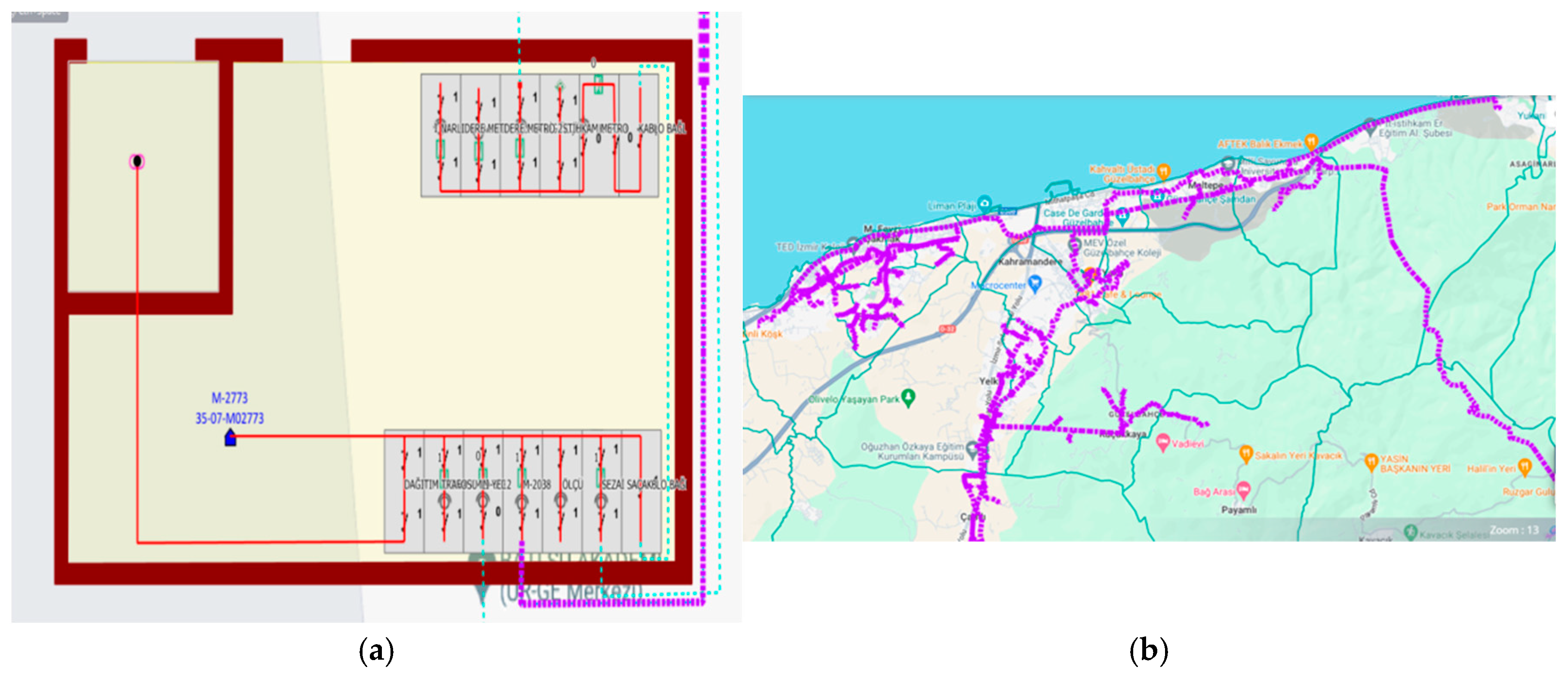
(i) The first data were taken from the M-2038 feeder with a line length of approximately 5850 km, located in Güzelbahçe district of Izmir. There are 146 transformers, including the 154/34.5 V medium voltage (MV) line in the M-2038 feeder of Izmir Güzelbahçe district and the M-2038 feeder output of the M-2773 cabin. There are 11,392 subscribers on the Güzelbahçe feeder. Visual diagrams of the feeder exit cabin and the energization zone of the relevant feeder are shown in Figure 2a and Figure 2b, respectively.
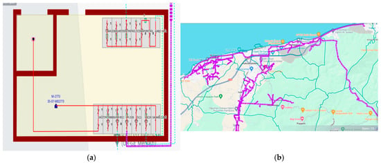
Figure 2.
Güzelbahçe district of Izmir. (a) Visual diagram of the M-2038 feeder output cabin. (b) Diagram of the M-2038 feeder energization zone.
(ii) The second data were taken from the Yenikent feeder with a line length of approximately 3850 km in Izmir-Bergama district. Izmir-Bergama district has 154/34.5 V MV lines and 50 transformers. A total of 1054 subscribers receive energy services from the M-2038 feeder. The cabin and energization zone diagrams of the Tekkedere DM-Yenikent Feeder is shown in Figure 3a and Figure 3b, respectively.

Figure 3.
Izmir-Bergama district. (a) Diagram of the Tekkedere DM—Yenikent feeder cabin. (b) Visual diagram of the Tekkedere DM—Yenikent energization zone.
For the dataset, approximately 1999 data points were recorded and labeled. A total of six inputs (Ia, Ib, Ic, Va, Vb, and Vc), consisting of the voltages and currents of three phases, were applied to the input of the created machine learning models. The types of faults recorded in the dataset are shown in Table 2.
- (b)
- Dataset 2: Public dataset
In this study, the public dataset labeled “Electrical Fault detection and classification” created within the MATLAB Simulink-based simulation framework was used [26,27]. A power system was modeled in MATLAB to simulate the fault analysis. In the power system, four generators rated at 11,000 V are positioned at both ends of each pair of transmission lines. Transformers were positioned at the middle point of the transmission line to simulate and examine various faults. The circuit was simulated under normal conditions and under various fault conditions, and the voltage and current values of the line were recorded at the output of the power system. For the dataset, approximately 12,000 data points were recorded and labeled. A total of six inputs (Ia, Ib, Ic, Va, Vb, and Vc), consisting of the voltages and currents of three phases, were applied to the input of the created machine learning models. The dataset includes different types of faults related to transmission lines. The fault types included in the dataset are shown in Table 2.
- (c)
- Dataset 3: Fault dataset generated using Simulink
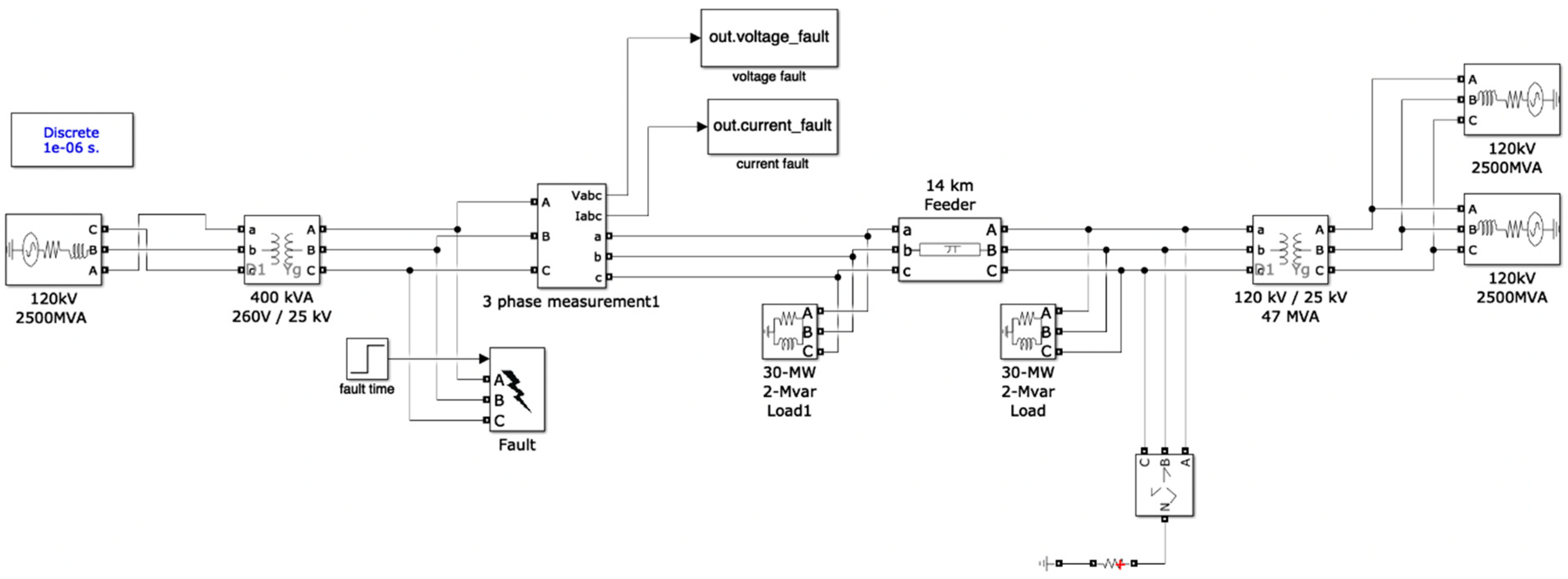
The Simulink of the power system was modeled to generate the dataset for fault analysis in MATLAB depicted in Figure 4. Three 25,000 MVA generators are used in the model power system to generate alternative energy. These generators are located at the start and end of the transmission line. Through the use of transformers that convert 120 kV to 25 kV, the generators’ 120 kV voltage is sent to a 28 km transmission line. Two 30 MW loads are present on the transmission line. The middle of the transmission line, at km 14, is where multiple faults are simulated to occur at different times. The voltage and current values of the line at the power system’s output were recorded while the circuit was simulated under both normal and different fault scenarios. The fault types included in the dataset are shown in Table 2.
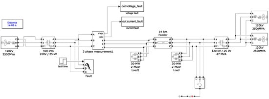
Figure 4.
A Simulink model was developed to generate the dataset.
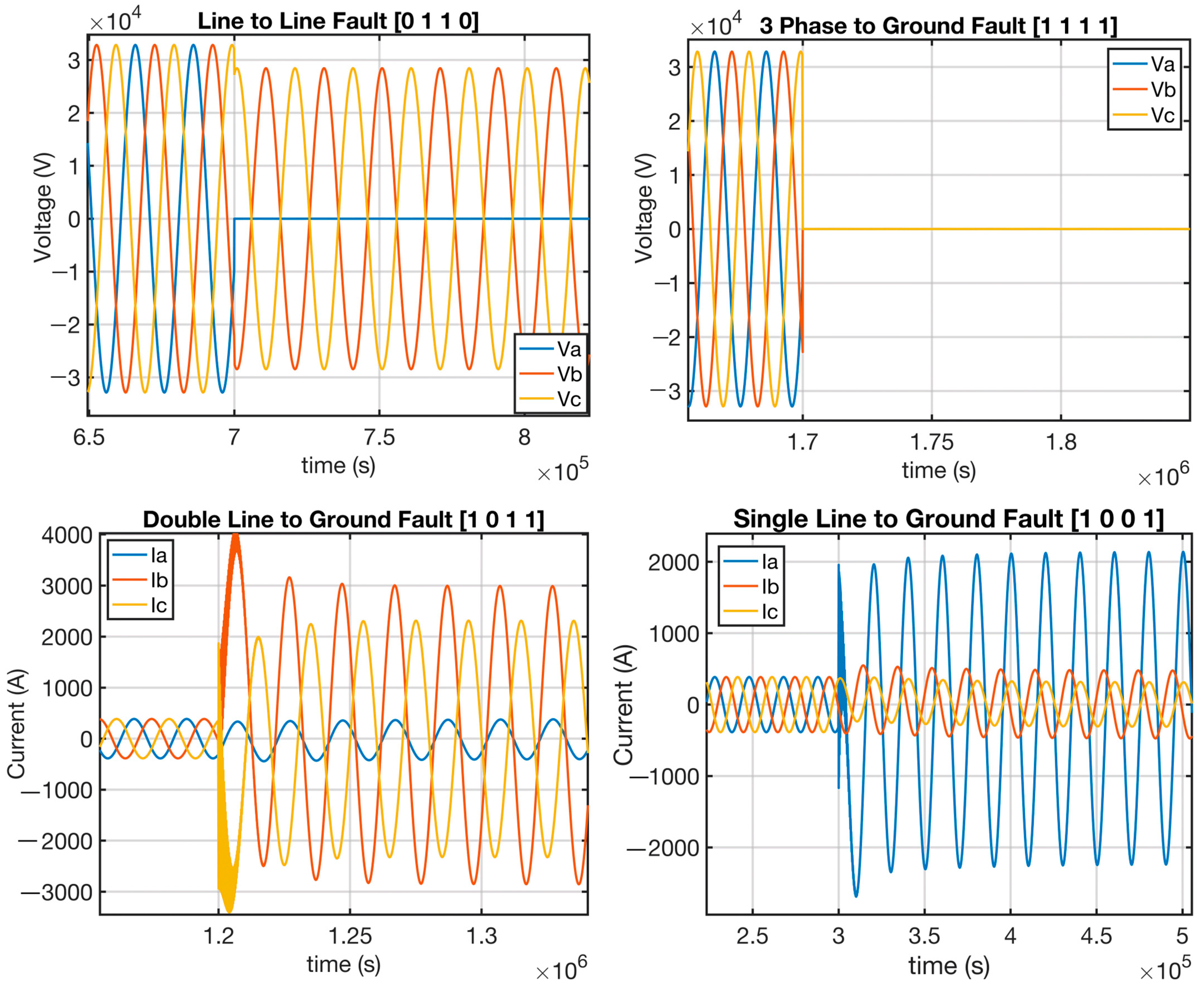
The study evaluated the results of symmetrical three-phase short-circuit faults as well as a single phase to ground, phase to phase, and phase to phase to ground asymmetric faults. Every failure type’s allowed occurrence time was within 0.1 s during the simulation’s total runtime of 1 s. Voltage and current graphs of nominal and fault conditions obtained during 1 s of operation are given in Figure 5.
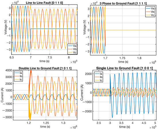
Figure 5.
Some of the voltage and current graphs during the transition from a nominal operating state to a faulty operating state.
For the dataset, approximately 19,999 data points were recorded and labeled. A total of six inputs (Ia, Ib, Ic, Va, Vb, and Vc), consisting of the voltages and currents of three phases, were applied to the input of the created machine learning models.
2.2. 1D Convolutional Neural Network Model
A convolutional neural network (CNN) is a deep learning methodology that was first designed to handle arrays that are two dimensions in size. The architecture can have multiple layers applied in order to discern various aspects within a two-dimensional image. Convolutional filters are used to extract various picture features at various resolutions, and the resulting output is then applied as the input for the following layer. Convolution, activation, and pooling layers are components of the CNN architecture. These three layers are often a collection of layers that are repeated in an attempt to attain the properties of two-dimensional arrays. In order to estimate continuous data in regression problems, a regression layer can be added to the end of the model.
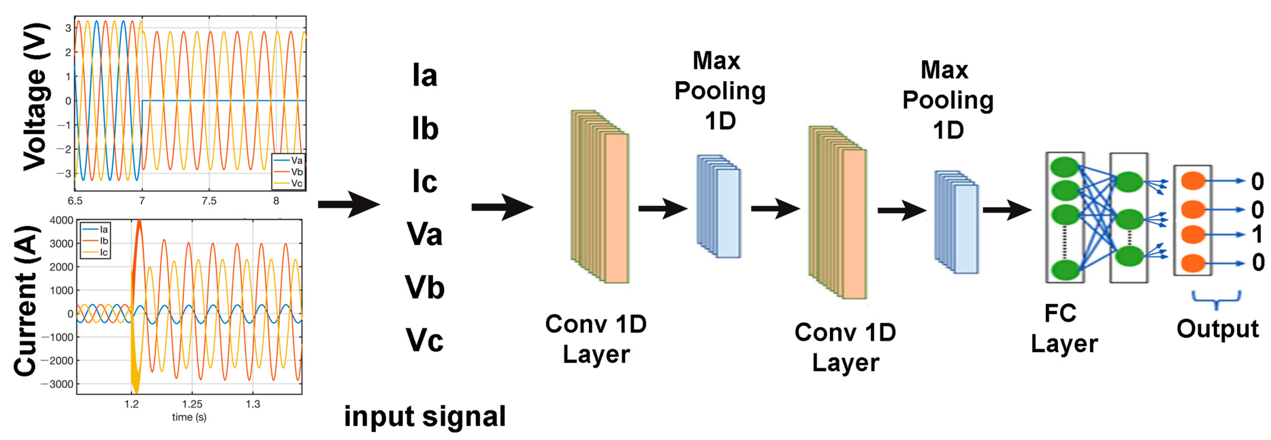
Modern machine learning methods, especially 1D CNNs and recurrent neural networks (RNNs), have proven to be extremely effective in solving difficult activity recognition and classification tasks in recent times [28,29,30]. The architecture of the 1D CNN model used in the article is shown in Figure 6.
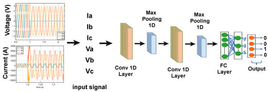
Figure 6.
The architecture of a 1D CNN model [29].
2.3. Normalization
In order to enhance algorithm efficiency, convergence speed, and model interpretability, particularly for algorithms that are sensitive to feature scales, normalization is a popular preprocessing step in machine learning. In this study, min-max normalization was used, and the mathematical expression can be represented by Equation (1) where x represents original values of all the samples.
2.4. Proposed Deep Learning Model for Fault Classification
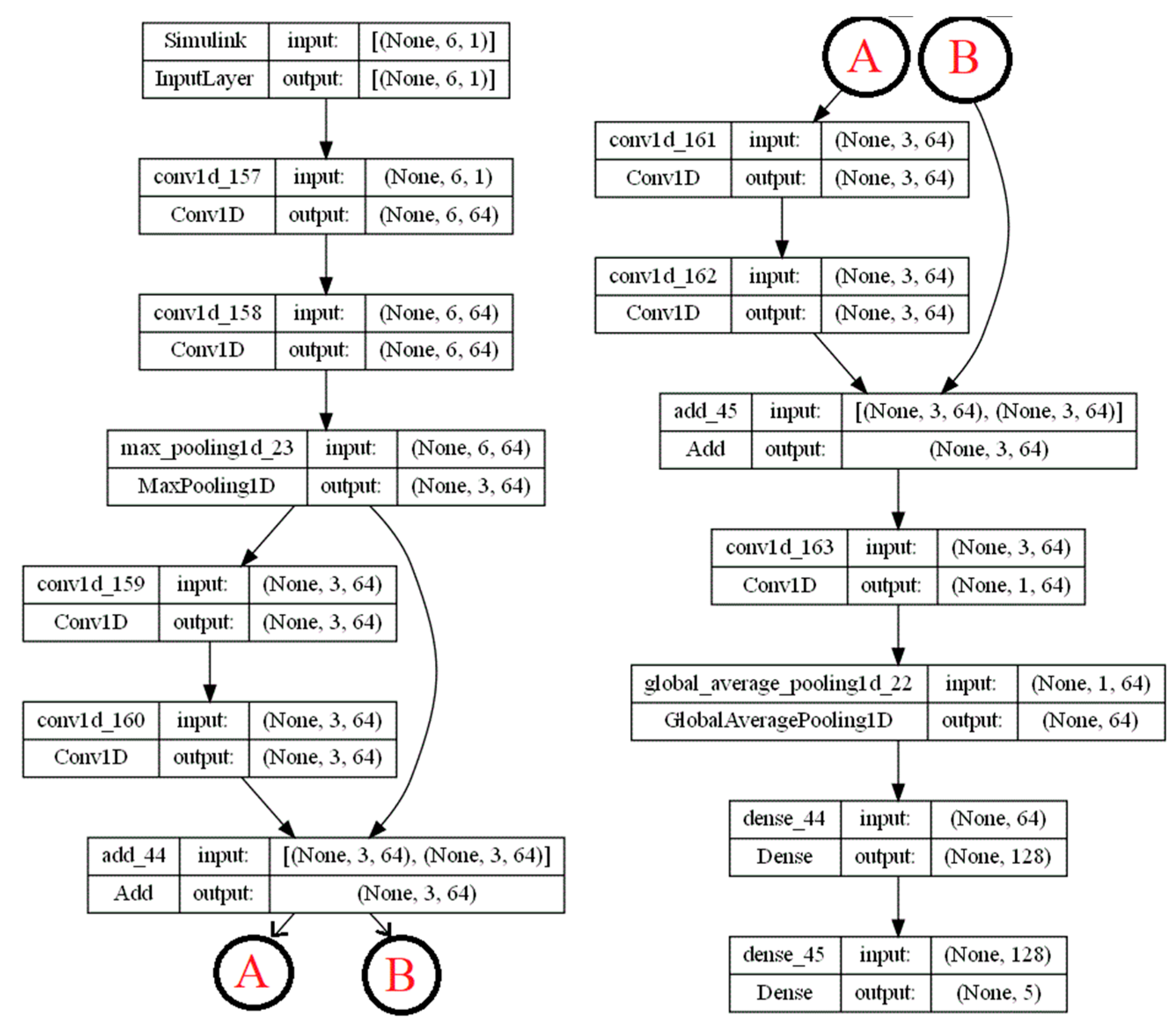
In this study, one-dimensional convolutional neural network (1D CNN) architecture, which is suitable for processing sequential data like time series or signals, was employed for fault classification in transmission lines. The 1D CNN based deep learning model architecture proposed in this study is shown in Figure 7, and its description is listed below.
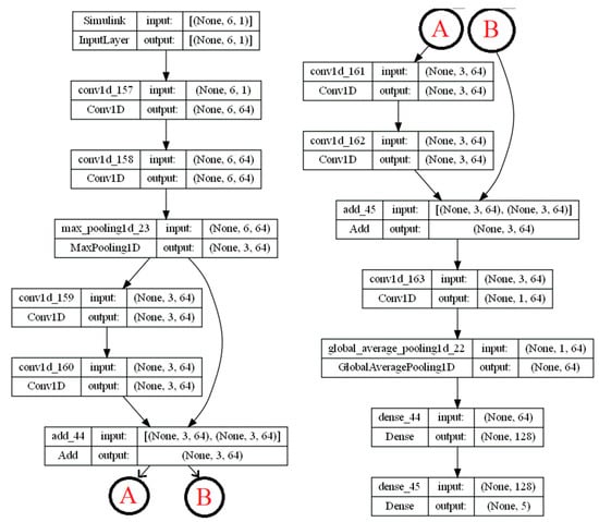
Figure 7.
Proposed deep learning model for fault classification.
- Keras, a high-level neural networks application programming interface (API) that runs on top of TensorFlow, is used to define the architecture of the model.
- First Block: Two convolutional layers (Conv1D) are applied successively to the input. Each convolutional layer has 64 filters with a filter size of three and ReLU activation function. The output of the second convolutional layer is passed through a max pooling layer (MaxPooling1D) with a pool size of two and “same” padding. This reduces the length of the sequence by half while retaining important features. This block also helps extract features from the input data.
- Second Block: Two convolutional layers are applied to the output of the first block. These layers have the same configuration as the layers in the first block.
- Residual Connection: The output of the second convolutional layer is added element-wise to the output of the first block. This creates a residual connection, allowing the network to learn residual mappings, which can make training deeper networks easier.
- Third Block: Two more convolutional layers are applied to the output of the second block. Again, the layers have the same configuration as before. Another residual connection is formed by adding the output of the second convolutional layer to the output of the second block.
- Final Layers: One more convolutional layer is applied to the output of the third block.
The output is then passed through a global average pooling layer, which computes the average of each feature map across the entire sequence. The output of the pooling layer is fed into a dense layer with 128 units and ReLU activation. Finally, the output layer consists of a dense layer for classification tasks, with as many units as the number of classes or outputs in the dataset.
2.5. Parameter Setting
Splitting data into training and test groups by numbers is still a controversial issue [15]. There is currently a lack of practical information on which strategy to choose under what circumstances when it comes to data creation for later training of machine learning models [31]. The 80:20 ratio is recommended in accordance with the Pareto principle [32]. Thus, 20% of the data is reserved for testing, while the remaining 80% is used for training. In the training stage, 20% of the training set is reserved for validation.
The model’s training parameters encompass various aspects crucial for effective training. The following is a list of additional hyperparameters to consider. Since it is a multi-class classification problem, Adam has been selected as the optimizer, and categorical cross-entropy has been selected as the loss function. The metric for evaluation is accuracy. The number of epochs, which is taken to be 100, determines the training time and the number of full passes in the dataset. In addition, the batch size, which is set to 32, determines the number of samples that are processed in each iteration before updating the model’s weights, thereby improving efficiency.
2.6. Assessment Criteria
In the literature, different performance metrics are used to determine the accuracy of classification models. In most scientific domains, the area under the receiver operating characteristic curve (ROC AUC) has become the accepted standard metric for assessing binary classifications. Binary classification is a typical activity that makes use of machine learning and computational statistics [33]. In this study, seven measures based on true positive (TP), true negative (TN), false positive (FP), and false negative (FN) were utilized. The formulas of measures are briefly defined as follows [13].
Accuracy () is the ratio of the sum of correct predictions to the total samples of dataset.
Precision (P) is the ratio of correct predictions of the positive class to the total positive predictions.
Recall (R), also called sensitivity, is the ratio of correct predictions of the positive class to the sum of correct predictions of the positive class and incorrect predictions of the negative class.
The F1 score is a weighted average of precision and recall. The F1 score is usually more valuable than accuracy, particularly if the underlying dataset has an uneven class distribution.
The confusion matrix summarizes the accuracy, specificity, recall, and precision and is used to measure the performance of a machine learning classification problem. In addition, it is an efficient tool for drawing receiver operating characteristic (ROC) curves and calculating the area under the ROC curve (AUC). The ROC curve is a graphical plot that demonstrates the characteristic capability of a binary classifier.
3. Results of the Model
3.1. Fault Classification
In this section, the classification outcomes of the proposed model, which was independently trained using all three datasets, are presented.
- (a)
- Results of the public dataset
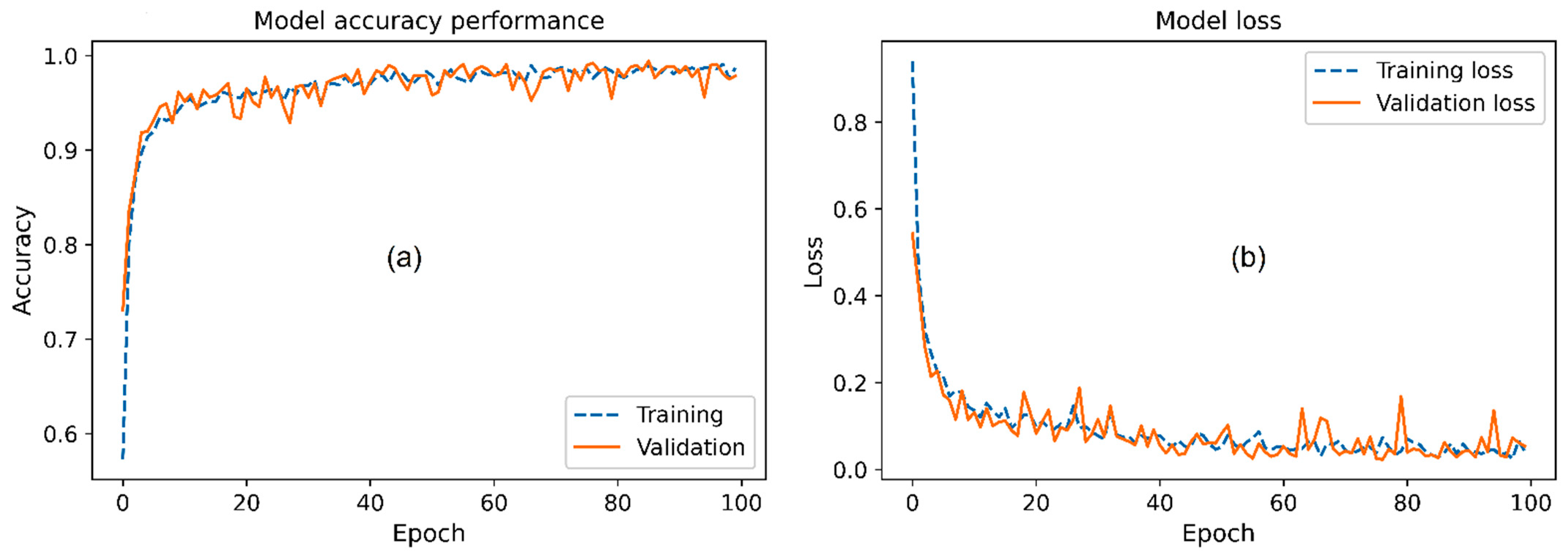
Figure 8a,b illustrates the graphs depicting the changes in accuracy and loss, respectively, during the training stage of the proposed model using the public dataset. It has been observed that as the number of epochs increases in the training process, the accuracy value gradually increases. On the other hand, the loss curve of the machine learning process shows that as the number of repetitions of the machine learning data increases, the loss function value gradually decreases.
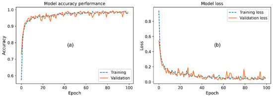
Figure 8.
(a) Accuracy performance of the proposed model using the public dataset. (b) The loss of the proposed model using the public dataset.
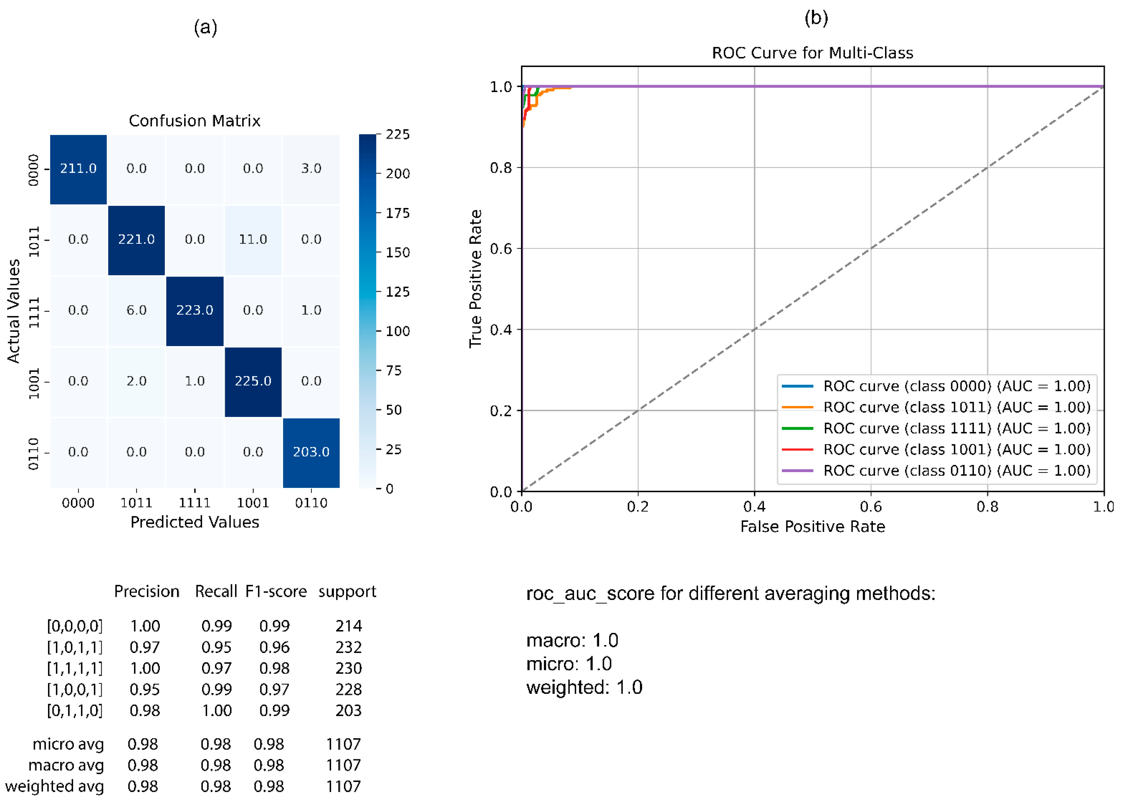
After the training stage of the model, the confusion matrix was calculated to determine the performance of the proposed model, and scores of different performance criteria using confusion matrix are presented in a table in Figure 9a with a classification report. Micro averages (avg) are useful when the classes are imbalanced, and it is important to have a better understanding of the model’s performance on the majority class. Therefore, it was observed that the micro avg values were 0.98.
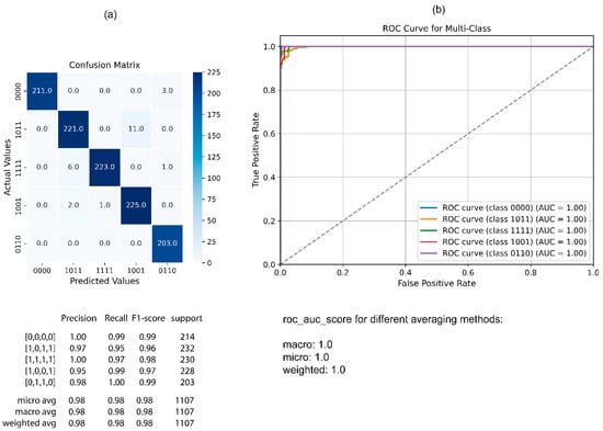
Figure 9.
(a) Confusion matrix of the public dataset with a classification report. (b) ROC curve of the public dataset.
ROC curves provide a comprehensive overview of the performance of a classification model across different threshold values. They plot the true positive rate (TPR) against the false positive rate (FPR) at various threshold settings. This allows for a visual comparison of the trade-offs between sensitivity and specificity. For these reasons, ROC curves were drawn for each class, and the resulting changes are shown in Figure 9b. As seen in the figure, the AUC value obtained for all classes was approximately 1.0.
- (b) Results of the dataset generated based on Simulink
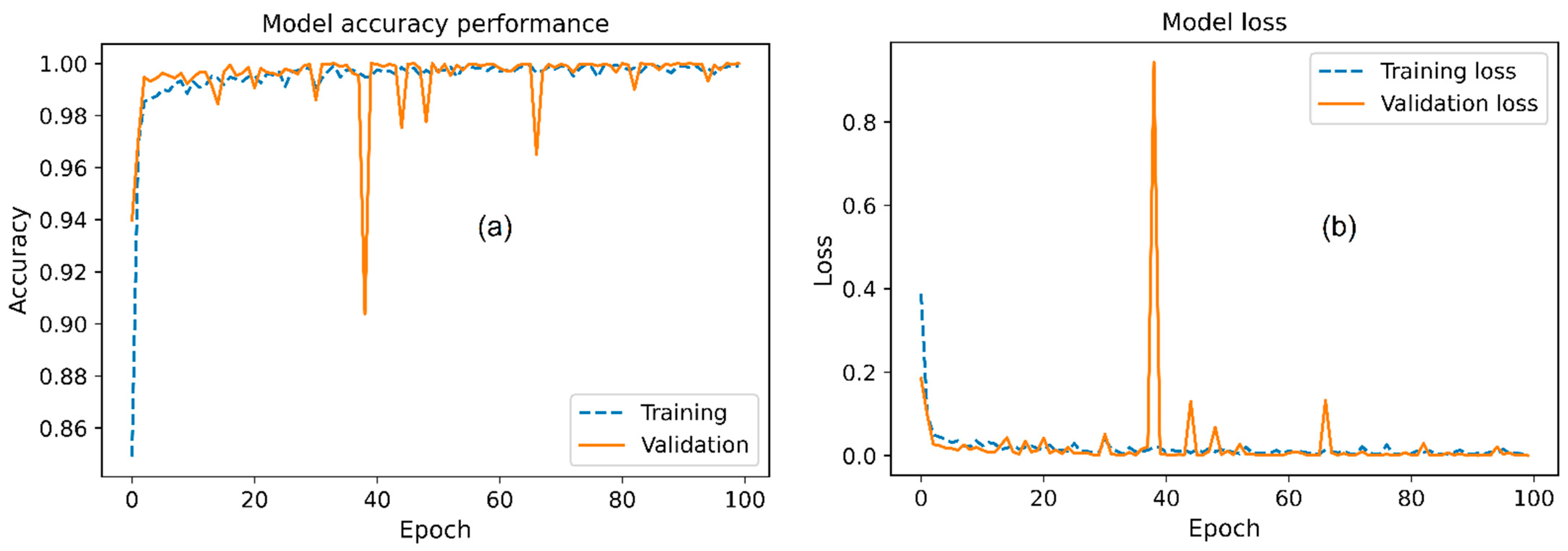
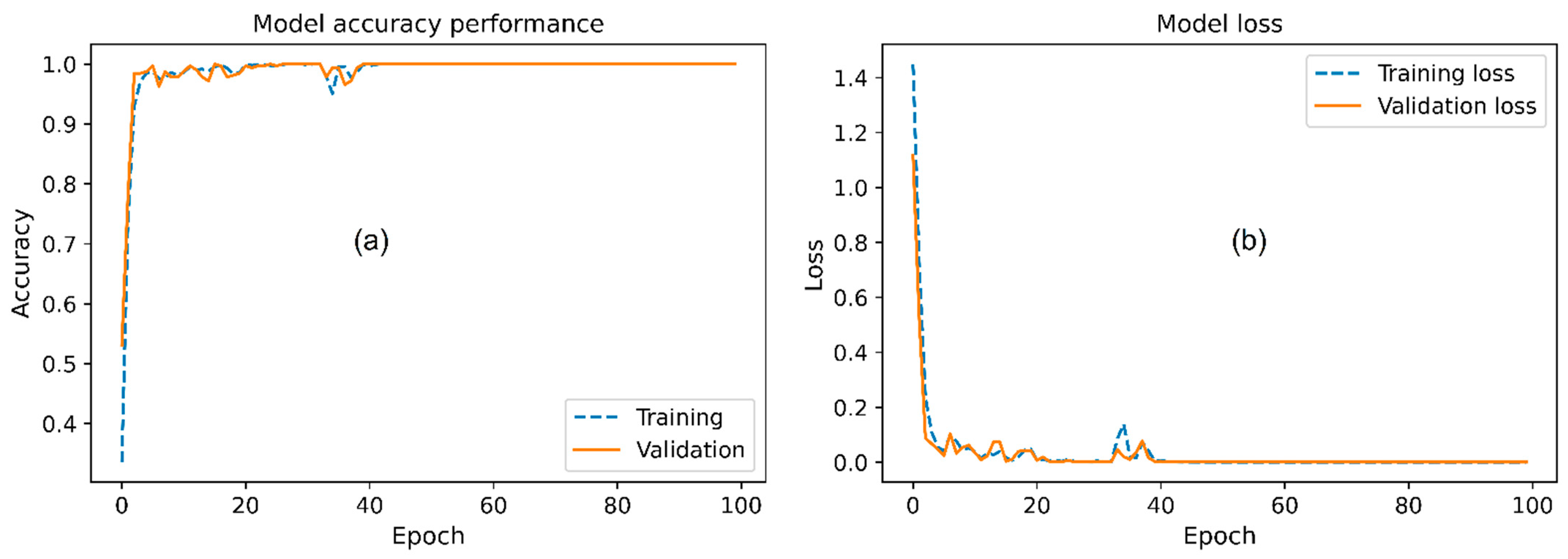
The generated Simulink dataset was utilized during the training stage to evaluate the proposed model. The variations in accuracy and loss parameters that were observed are illustrated in Figure 10a and Figure 10b, respectively. The presence of patterns with similar characteristics in the validation set caused the patterns to be classified incorrectly. In addition, this situation caused a sudden drop in the accuracy graph and a sudden rise in the loss graph, as can be seen in Figure 10. As noted in the public dataset, it has been observed that as the number of epochs increases in the training process, the accuracy value gradually increases. However, when compared to the public dataset, it can be seen that high accuracy can be achieved with fewer epochs. The loss curve indicates that the loss function value is reduced with machine learning data repetitions.
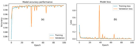
Figure 10.
(a) Accuracy performance of the proposed model for the Simulink dataset. (b) The loss of proposed model for the Simulink dataset.
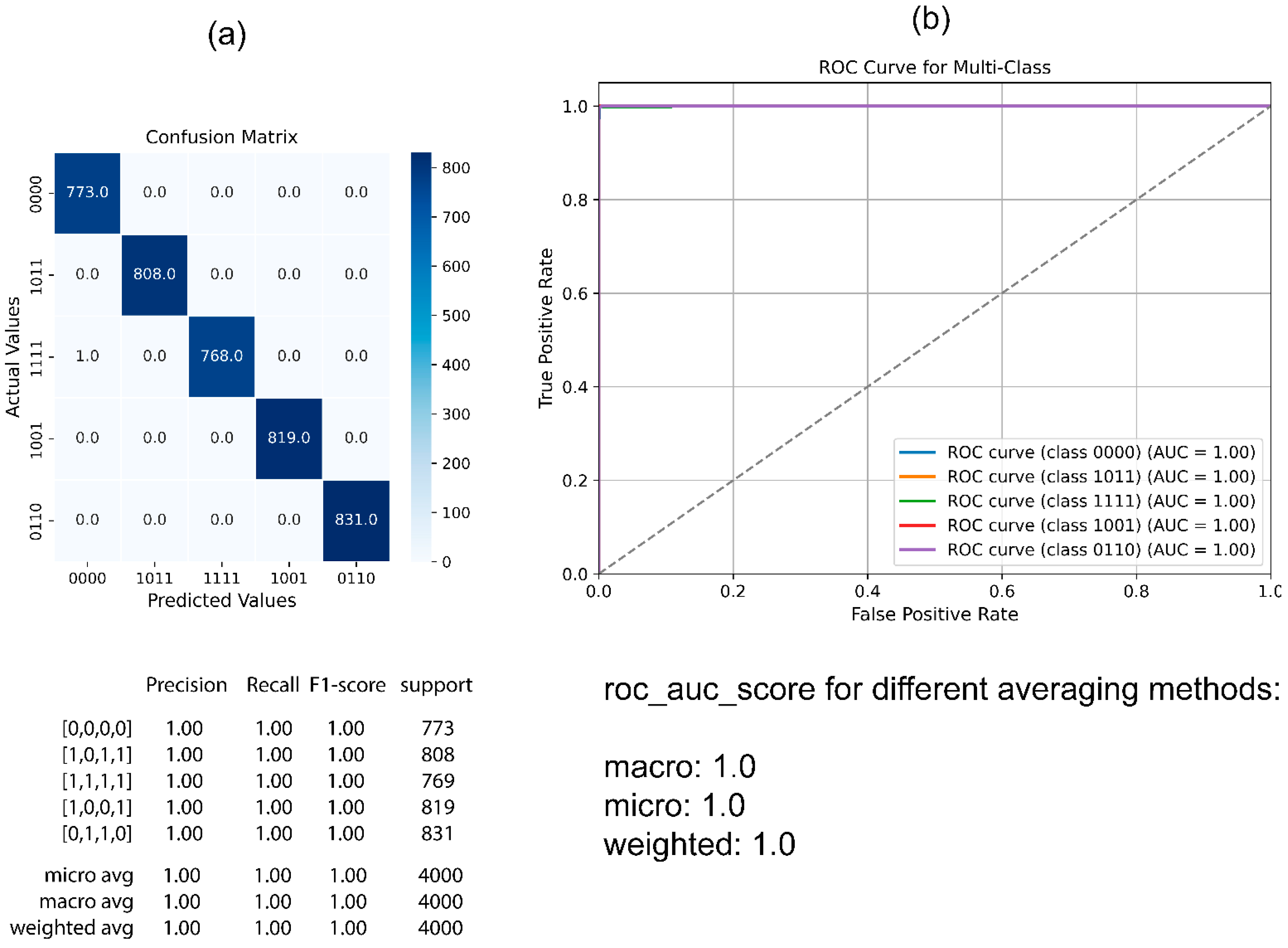
After the training stage of the model, the confusion matrix with a classification report was calculated to determine the performance of the proposed model depicted in Figure 11a. It was observed that the micro avg values were 1.0. ROC curves were drawn for each class, and the resulting changes are shown in Figure 11b. As seen in the figure, the AUC value obtained for all classes was approximately 1.0.
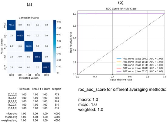
Figure 11.
(a) Confusion matrix of the Gediz dataset with a classification report. (b) ROC curve of the real dataset.
- (c) Results of the real (Gediz) dataset
In the training stage, the real dataset was utilized in the proposed model, and Figure 12a,b illustrates the changes that were noticed in terms of accuracy and loss parameters, respectively. As noted in the public and Simulink datasets, it has been observed that as the number of epochs increases in the training process, the accuracy value gradually increases. However, it appears that accuracy is achieved with fewer iterations compared to the public and Simulink datasets. The loss curve indicates that the loss function value is reduced with machine learning data iterations.
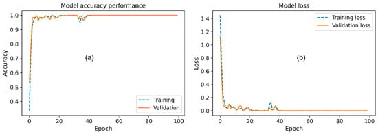
Figure 12.
(a) Accuracy performance of the proposed model for the real dataset. (b) The loss of the proposed model for the real dataset.
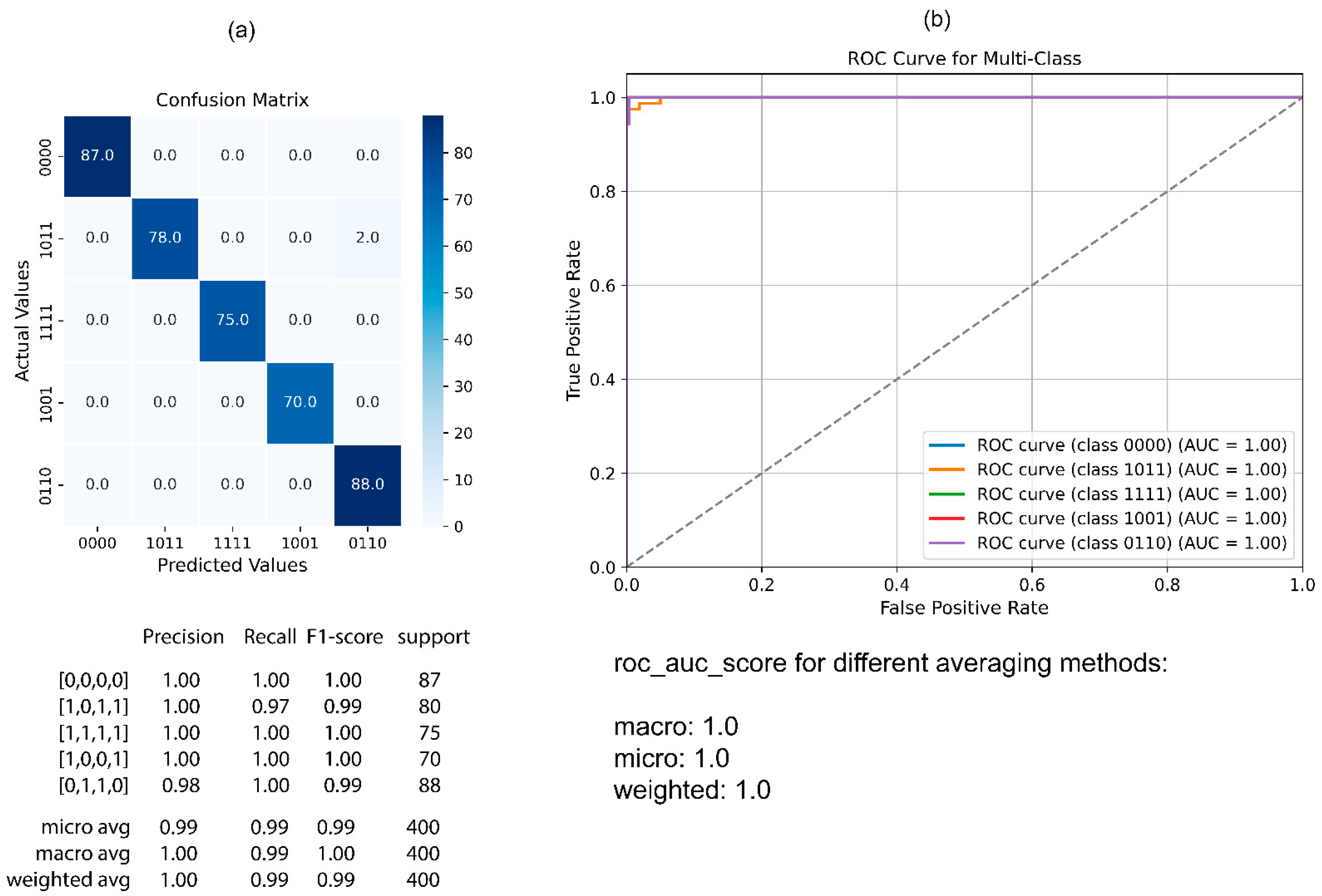
After the training stage of the model, the confusion matrix with a classification report was generated to determine the performance of the proposed model depicted in Figure 13a. It was observed that the micro avg values were 0.99. ROC curves were drawn for each class, and the resulting changes are shown in Figure 13b. As seen in the figure, the AUC value obtained for all classes was approximately 1.0.
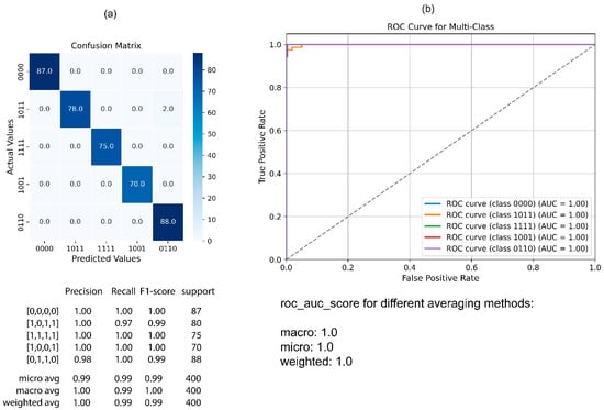
Figure 13.
(a) Confusion matrix of the real dataset with a classification report. (b) ROC curve of the real dataset.
3.2. Comparison with State-of-the-Art Models
The main purpose of this paper is to design a deep network model to classify the fault in transmission lines based on real, generated, and public datasets. We can see that different studies have been carried out in the literature for similar purposes. To demonstrate the superiority of the proposed method, existing state-of-the-art methods for fault classification were also compared, as shown in Table 3. The following information about some basic studies is included in the table: methods, approaches for generating the dataset, their objectives, performance criteria, and the results of the proposed models.
The dataset is one of the important parameters we see in studies. With these datasets, analysis and evaluation of fault types are made. It is observed that in the literature, MATLAB-Simulink [17,22,34] or OpenDSS-G [23] software is used to generate datasets. In addition to this, the research utilize public datasets [25,35] as well as datasets acquired with field measurements [35,36,37]. The models are then trained utilizing a variety of techniques and the datasets that have been provided. Using the trained models, fault detection or fault classification can be effectively accomplished. The findings, as shown in Table 3, are satisfactory, particularly when compared to the performance requirements established for fault classification.
Providing real data requires businesses to have the necessary hardware and software. This increases operating expenses. Therefore, obtaining data in businesses is a very difficult process. For that reason, it is mentioned in the studies [38] that real data will be used, especially within the scope of future studies. However, in this study, fault classification was made using real data. Apart from this, a synthetic dataset was produced with the model designed in MATLAB-Simulink and public dataset was used in this study.
Utilizing simulation tools to generate datasets results in the data values being ideal. Performing analysis with ideal data causes a disadvantage. To prevent this, realistic datasets are created by adding white noise, such as 20 dB or 30 dB, to the datasets [20].
The real dataset, the dataset generated with Simulink, and the public dataset were used separately to train and evaluate the model that was suggested in this study, and the model was found to have a strong structure based on the results. The public dataset used in this study was also used in the reference study [25], and it was found that the outcomes of this study yielded better results because of the proposed model.

Table 3.
Comparison of proposed model with other state-of-the-art models for fault classification.
Table 3.
Comparison of proposed model with other state-of-the-art models for fault classification.
| Ref. | Method | Dataset—Purpose | Criteria/Results |
|---|---|---|---|
| [34] | Deep Adversarial Transfer Learning | Generated with simulink—Fault classification | Acc./98.05 |
| [22] | LSTM | Generated with simulink—Fault classification | Acc./ideal 100%, 99.77% with 30 dB and 99.55% with 20 dB for 11 classes |
| [23] | ANN | Generated dataset (IEEE-13 bus)—Fault classification | Acc./avg. 99.6 for 10 classes |
| [17] | LSTM, LSTM-WR, ANN | Generated dataset with Simulink—Fault classification | Acc./43.33, 100, and 99.98, respectively |
| [25] | SVM, KNN, Decision Tree, Random Forest | Public dataset (four columns as fault status)—Fault detection | Acc./0.85, 0.83, 0.83, and 0.84, respectivly |
| [39] | ANFIS | Generated dataset (IEEE-37 bus)—Fault detection, classification and location | Acc./99.9 |
| Proposed model | 1D CNN-based Deep Learning Structure | Real/generated with Simulink/public datasets—Fault classification | Micro avg./0.99, 1.00, and 0.98, respectively |
4. Conclusions
The main purpose of this paper is to design a deep network model to classify the faults in transmission lines based on a real dataset, a dataset generated with Simulink, and a public dataset. The findings obtained in our study are listed below.
- The results obtained in fault classification are at an acceptable level compared to the results obtained in the literature.
- Not only synthetic but also real data were used in this study. It has been observed that the created model can be used successfully for both real data and synthetic data.
- The proposed model shows an impressive result for all datasets. Hence, it can be said that the proposed model performance is independent of the transmission line configuration.
- It also will be tested with 3 different sets of data, which consist of real, generated, and public datasets to measure the robustness of the network.
Author Contributions
Conceptualization, Y.B.Y. and O.T.; methodology, Y.B.Y.; software, Y.B.Y. and O.T.; validation, Y.B.Y.; formal analysis, O.T.; investigation, Y.B.Y.; resources, Y.B.Y.; data curation, O.T.; writing—original draft preparation, Y.B.Y. and O.T.; writing—review and editing, Y.B.Y.; visualization, O.T.; supervision, Y.B.Y.; project administration, Y.B.Y. and O.T.; funding acquisition, Y.B.Y. All authors have read and agreed to the published version of the manuscript.
Funding
This research received no external funding.
Institutional Review Board Statement
Not applicable.
Informed Consent Statement
Not applicable.
Data Availability Statement
The raw data supporting the conclusions of this article will be made available by the authors on request.
Acknowledgments
We would like to thank Gediz Electricity Distribution Company affiliated with TEDAŞ for the data obtained with the permission received from the Electricity Distribution Company.
Conflicts of Interest
Author Ozan Turanli was employed by the company GDZ Electrical Energy Inc. The remaining author declares that the research was conducted in the absence of any commercial or financial relationships that could be construed as a potential conflict of interest.
References
- Radojevic, Z.M.; Kim, C.H.; Popov, M.; Preston, G.; Terzija, V. New Approach for Fault Location on Transmission Lines Not Requiring Line Parameters. In Proceedings of the International Conference on Power Systems Transients IPST, Kyoto, Japan, 2–6 June 2009. [Google Scholar]
- Izykowski, J. Power System Faults; PRINTPAP: Łódź, Poland, 2011; ISBN 978-83-62098-80-4. [Google Scholar]
- Stefanidou-Voziki, P.; Sapountzoglou, N.; Raison, B.; Dominguez-Garcia, J. A review of fault location and classification methods in distribution grids. Electr. Power Syst. Res. 2022, 209, 108031. [Google Scholar] [CrossRef]
- Jia, K.; Bi, T.; Ren, Z.; Thomas, D.W.P.; Sumner, M. High frequency impedance based fault location in distribution system with DGs. IEEE Trans. Smart Grid 2018, 9, 807–816. [Google Scholar] [CrossRef]
- Srivastava, A.; Parida, S. Data driven approach for fault detection and Gaussian process regression based location prognosis in smart AC microgrid. Electr. Power Syst. Res. 2022, 208, 107889. [Google Scholar] [CrossRef]
- Ozcanli, A.K.; Yaprakdal, F.; Baysal, M. Deep learning methods and applications for electrical power systems: A comprehensive review. Int. J. Energy Res. 2020, 44, 7136–7157. [Google Scholar] [CrossRef]
- Ibrahim, M.S.; Dong, W.; Yang, Q. Machine learning driven smart electric power systems: Current trends and new perspectives. Appl. Energy 2020, 272, 115237. [Google Scholar] [CrossRef]
- Miao, X.; Liu, X.; Chen, J.; Zhuang, S.; Fan, J.; Jiang, H. Insulator detection in aerial images for transmission line inspection using single shot multibox detector. IEEE Access 2019, 7, 9945–9956. [Google Scholar] [CrossRef]
- Anjaiah, K.; Dash, P.K.; Sahani, M. A new protection scheme for PV-wind based DC-ring microgrid by using modified multifractal detrended fluctuation analysis. Prot. Control. Mod. Power Syst. 2022, 7, 8. [Google Scholar] [CrossRef]
- Sampedro, C.; Rodriguez-Vazquez, J.; Rodriguez-Ramos, A.; Car- rio, A.; Campoy, P. Deep learning-based system for automatic recognition and diagnosis of electrical insulator strings. IEEE Access 2019, 7, 101283–101308. [Google Scholar] [CrossRef]
- Wang, J.; Pinson, P.; Chatzivasileiadis, S.; Panteli, M.; Strbac, G.; Terzija, V. On Machine learning-based techniques for future sustainable and resilient energy systems. IEEE Trans. Sustain. Energy 2023, 14, 1230–1241. [Google Scholar] [CrossRef]
- Vaish, R.; Dwivedi, U.; Tewari, S.; Tripathi, S. Machine learning applications in power system fault diagnosis: Research advancements and perspectives. Eng. Appl. Artif. Intell. 2021, 106, 104504. [Google Scholar] [CrossRef]
- Goni, M.F.; Nahiduzzaman, M.; Anower, M.; Rahman, M.; Islam, M.; Ahsan, M.; Haider, J.; Shahjalal, M. Fast and accurate fault detection and classification in transmission lines using extreme learning machine. E-Prime Adv. Electr. Eng. Electron. Energy 2023, 3, 100107. [Google Scholar] [CrossRef]
- Manojna; Sridhar, H.S.; Nikhil, N.; Kumar, A.; Amrit, P. Fault detection and classification in power system using machine learning [Paper presentation]. In Proceedings of the Second International Conference on Smart Electronics and Communication (ICOSEC), Trichy, India, 7–9 October 2021. [Google Scholar]
- Wadi, M. Fault detection in power grids based on improved supervised machine learning binary classification. J. Electr. Eng. 2021, 72, 315–322. [Google Scholar] [CrossRef]
- Ahmad, T.; Madonski, R.; Zhang, D.; Huang, C.; Mujeeb, A. Data-driven probabilistic machine learning in sustainable smart energy/smart energy systems: Key developments, challenges, and future research opportunities in the context of smart grid paradigm. Renew. Sustain. Energy Rev. 2022, 160, 112128. [Google Scholar] [CrossRef]
- Shukla, P.K.; Deepa, K. Deep learning techniques for transmission line fault classification—A comparative study. Ain Shams Eng. J. 2024, 15, 102427. [Google Scholar] [CrossRef]
- Tirnovan, R.-A.; Cristea, M. Advanced techniques for fault detection and classification in electrical power transmission systems: An overview. In Proceedings of the 2019 8th International Conference on Modern Power Systems (MPS), Cluj Napoca, Romania, 21–23 May 2019; IEEE: Piscataway, NJ, USA, 2019; pp. 1–10. [Google Scholar]
- Ajagekar, A.; You, F. Quantum computing based hybrid deep learning for fault diagnosis in electrical power systems. Appl. Energy 2021, 303, 117628. [Google Scholar] [CrossRef]
- Fahim, S.R.; Sarker, S.K.; Muyeen, S.; Das, S.K.; Kamwa, I. A deep learning based intelligent approach in detection and classification of transmission line faults. Int. J. Electr. Power Energy Syst. 2021, 133, 107102. [Google Scholar] [CrossRef]
- Belagoune, S.; Bali, N.; Bakdi, A.; Baadji, B.; Atif, K. Deep learning through LSTM classification and regression for transmission line fault detection, diagnosis and location in large-scale multi-machine power systems. Measurement 2021, 177, 109330. [Google Scholar] [CrossRef]
- Omar AM, S.; Osman, M.K.; Ibrahim, M.N.; Hussain, Z.; Abidin, A.F. Fault classification on transmission line using LSTM network. Indones. J. Electr. Eng. Comput. Sci. 2020, 20, 231–238. [Google Scholar]
- Tokel, H.A.; Al Halaseh, R.; Alirezaei, G.; Mathar, R. A new approach for machine learning-based fault detection and classification in power systems. In Proceedings of the 2018 IEEE Power & Energy Society Innovative Smart Grid Technologies Conference (ISGT), Washington, DC, USA, 19–22 February 2018; IEEE: Piscataway, NJ, USA, 2018; pp. 1–5. [Google Scholar]
- Nasrin, M.A.M.; Omar, A.M.S.; Ramli, S.S.M.; Ahmad, A.R.; Jamaludin, N.F.; Osman, M.K. Deep Learning Approach for Transmission Line Fault Classification. In Proceedings of the 2021 11th IEEE International Conference on Control System, Computing and Engineering (ICCSCE), Penang, Malaysia, 27–28 August 2021; IEEE: Piscataway, NJ, USA, 2021; pp. 164–169. [Google Scholar]
- Goswami, T.; Roy, U.B. Predictive model for classification of power system faults using machine learning. In Proceedings of the TENCON 2019—2019 IEEE Region 10 Conference (TENCON), Kerala, India, 17–20 October 2019; IEEE: Piscataway, NJ, USA, 2019; pp. 1881–1885. [Google Scholar]
- GDZ Electrical Energy Inc. GDZ Electricity Distribution Inc. Geographic Information System Software (EDABİS); GDZ Electrical Energy Inc.: Bornova Izmir, Turkiye, 2024. [Google Scholar]
- Jamil, M.; Sharma, S.K.; Singh, R. Fault detection and classification in electrical power transmission system using artificial neural network. SpringerPlus 2015, 4, 334. [Google Scholar] [CrossRef]
- Alhanaf, A.S.; Farsadi, M.; Balik, H.H. Fault Detection and Classification in Ring Power System with DG Penetration Using Hybrid CNN-LSTM. IEEE Access 2024, 12, 59953–59975. [Google Scholar] [CrossRef]
- Alsumaidaee, Y.A.M.; Paw, J.K.S.; Yaw, C.T.; Tiong, S.K.; Chen, C.P.; Yusaf, T.; Benedict, F.; Kadirgama, K.; Hong, T.C.; Abdalla, A.N.; et al. Fault detection for medium voltage switchgear using a deep learning hybrid 1D-CNN-LSTM model. IEEE Access 2023, 11, 97574–97589. [Google Scholar] [CrossRef]
- Khattak, K.D.; Choudhry, M.; Feliachi, A. Fault Classificaton and Location in Power Distribution Networks using 1D CNN with Residual Learning. In Proceedings of the 2024 IEEE Power & Energy Society Innovative Smart Grid Technologies Conference (ISGT), Bengaluru, India, 10–13 November 2024; IEEE: Piscataway, NJ, USA, 2024; pp. 1–5. [Google Scholar]
- Amini, M.; Sharifani, K.; Rahmani, A. Machine learning model towards evaluating data gathering methods in manufacturing and mechanical engineering. Int. J. Appl. Sci. Eng. Res. 2023, 15, 349–362. [Google Scholar]
- Elattar, E.E.; Shaheen, A.M.; El-Sayed, A.M.; El-Sehiemy, R.A.; Ginidi, A.R. Optimal Operation of Automated Distribution Networks Based-MRFO Algorithm. IEEE Access 2021, 9, 19586–19601. [Google Scholar] [CrossRef]
- Chicco, D.; Jurman, G. The Matthews correlation coefficient (MCC) should replace the ROC AUC as the standard metric for assessing binary classification. BioData Min. 2023, 16, 4. [Google Scholar] [CrossRef]
- Han, J.; Miao, S.H.; Yin, H.R.; Guo, S.Y.; Wang, Z.X.; Yao, F.X.; Lin, Y.J. Deep-Adversarial-Transfer Learning Based Fault Classification of Power Lines in Smart Grid. IOP Conf. Ser. Earth Environ. Sci. 2021, 701, 012074. [Google Scholar] [CrossRef]
- Elmasry, W.; Wadi, M. Detection of Faults in Electrical Power Grids Using an Enhanced Anomaly-Based Method. Arab. J. Sci. Eng. 2022, 47, 14899–14914. [Google Scholar] [CrossRef]
- Zhang, S.; Wang, Y.; Liu, M.; Bao, Z. Data-Based Line Trip Fault Prediction in Power Systems Using LSTM Networks and SVM. IEEE Access 2017, 6, 7675–7686. [Google Scholar] [CrossRef]
- Yan, S.; Gao, L.; Wang, W.; Cao, G.; Han, S.; Wang, S. An algorithm for power transmission line fault detection based on improved YOLOv4 model. Sci. Rep. 2024, 14, 5046. [Google Scholar] [CrossRef]
- Shiddieqy, H.A.; Hariadi, F.I.; Adiono, T. Power Line Transmission Fault Modeling and Dataset Generation For AI Based Automatic Detection. In Proceedings of the 2019 International Symposium on Electronics and Smart Devices (ISESD), Badung, Indonesia, 8–9 October 2019; pp. 1–5. [Google Scholar]
- Souhe FG, Y.; Boum, A.T.; Ele, P.; Mbey, C.F.; Kakeu, V.J.F. Fault detection, classification and location in power distribution smart grid using smart meters data. J. Appl. Sci. Eng. 2022, 26, 23–34. [Google Scholar] [CrossRef]
Disclaimer/Publisher’s Note: The statements, opinions and data contained in all publications are solely those of the individual author(s) and contributor(s) and not of MDPI and/or the editor(s). MDPI and/or the editor(s) disclaim responsibility for any injury to people or property resulting from any ideas, methods, instructions or products referred to in the content. |
© 2024 by the authors. Licensee MDPI, Basel, Switzerland. This article is an open access article distributed under the terms and conditions of the Creative Commons Attribution (CC BY) license (https://creativecommons.org/licenses/by/4.0/).


