Optimization of Rotary Drilling Rig Mast Structure Based on Multi-Dimensional Improved Salp Swarm Algorithm

Abstract

The mast is a critical component of rotary drilling rigs, which has a cross-section consisting of a rectangular shape formed by two web plates and two flange plates. Structural optimization of the mast is necessary to address the issue of excessive weight. The shortcomings of the traditional structural optimization algorithms are summarized as follows: the optimized steel plate thickness is a non-integer, where rounding upwards may increase the cost to a certain extent, but it can ensure the safety of the structure; rounding downwards its load carrying capacity may not satisfy the requirements, and thus a novel Salp Swarm Algorithm is proposed to solve the optimization problem. First, this study improves the initialization and update strategy in the traditional Salp Swarm Algorithm. In order to obtain a solution for engineering, an innovative multi-dimensional running comparison is carried out. Secondly, the optimization model of rotary drilling rigs is established based on the division of the working conditions. The objective function of the optimization model is to minimize the weight of the mast while considering the constraints of strength, stiffness, stability, and welding process. Finally, the proposed optimization algorithm and the established optimization model are applied to optimize the design of the mast for a rotary drilling rig. The empirical results demonstrate that the weight of the mast has been reduced by 20%. In addition, the Improved Salp Swarm Algorithm exhibits higher solution quality, faster iteration capability, and extreme stability in optimizing welded box sections compared to the conventional algorithm. The example shows that the Improved Salp Swarm Algorithm is applicable to the optimization problem of box sections.

1. Introduction

The increasing number of piling projects and increasingly high quality requirements contribute to the high demand of construction machinery, which is one of the key factors in determining the quality of the project. A rotary drilling rig, a popular choice in the market, is a kind of specialized piling engineering machinery with a wide range of advantages, such as low noise, high efficiency, minimal environmental pollution and various other benefits. However, the existing rotary drilling rig suffers from high energy consumption and poor economic efficiency, which is in urgent need of improvement.

The mast, as an important supporting member for the power head, drill pipe, drill bit, etc., is the skeleton of the rotary drilling rig. The weight has a large impact on the quality and performance of the whole machine, and its use directly determines the working condition of the whole rotary drilling rig, as it is subjected to complex loading conditions during operation. Consequently, the mast is susceptible to potential damage, leading to high maintenance costs and resource waste. Therefore, research on the lightweight nature of the mast structure of rotary drilling rigs is of paramount importance. In this study, the mast is selected as the research object.

Numerous studies have been conducted on the optimization of welded box sections for weight reduction. For example, Savković, M.M. et al. [1] optimized the main girder box section of a single-girder bridge crane, taking weight reduction of the girder as the objective and considering constraints, including strength, stability, stiffness and cost-effective, and used various bio-inspired algorithms to verify the feasibility of the method. Cheng, B. et al. [2] used a first-order optimization method based on finite element analysis with weight as the objective function and the cost increase due to steel strength enhancement was considered, and then the parameters such as stiffness were set as the constraint function, and finally, the results showed that the optimum weight of the bowtie truss was less than that of the conventional truss under the premise that the steel strength had been moderately enhanced. Qisong Qi et al. [3] proposed a lightweight design method for crane steel structures to address issues like heavy self-weight, high energy consumption, and costs. The method employs the multi-specular reflection algorithm (M-SRA), which improves computational efficiency over traditional algorithms. M-SRA demonstrated better global search capabilities, providing an effective approach for green lightweight design in mechanical products. Goran V. Pavlović et al. [4] optimized the weight of bridge crane main girders with a non-symmetric box-like cross-section. Using Eurocodes for strength analysis and the Water Evaporation Optimization (WEO) algorithm, the study demonstrates weight reductions of 24.43% to 34.73%. Thanh Cuong-Le et al. [5] proposed the New Movement Strategy Cuckoo Search (NMS-CS) algorithm, featuring Lévy distribution-based step lengths and orientation parameter control for improved flexibility, convergence, and accuracy. Benchmarking showed NMS-CS outperformed traditional algorithms. Its application to engineering cases, like spring design, pressure vessel design, and welded beam design, highlights its efficacy in solving constrained optimization problems.

Kaveh, A. et al. [6] introduced an improved ant colony optimization (IACO) algorithm for constrained engineering design, incorporating a sub-optimization mechanism (SOM) that updates the search space efficiently. By reducing pheromone vectors, decision variables, and search space, IACO with SOM accelerated optimization without compromising solution accuracy, demonstrating its effectiveness in complex engineering problems with both discrete and continuous variables. Goran Pavlović et al. [7] focused on optimizing the main girder design of a double beam bridge crane with an asymmetric box cross-section, utilizing the Moth-Flame Optimization (MFO) algorithm. This innovative population-based metaheuristic method addressed a multicriteria optimization problem by considering constraints such as strength, local stability of girder components, global stability, deflections, and oscillation periods. The study demonstrated significant material savings ranging from 19.42% to 25.49%. Mohammad Hijjawi et al. [8] focused on optimizing the main girder design of a double beam bridge crane using the Moth–Flame Optimization (MFO) algorithm. This study addressed a multicriteria optimization problem, considering constraints such as strength, local and global stability, deflections, and oscillation periods. The results showed material savings of 19.42% to 25.49%, highlighting the algorithm’s efficiency in managing multiple variables and achieving optimal solutions quickly. Mohamed Abdel-Basset et al. [9] introduced a hybrid krill herd (CSKH) approach for structural optimization, combining the Krill Herd algorithm (KH) with the KU/KA operator from the cuckoo search algorithm (CS). CSKH employs a greedy selection scheme and replaces some of the worst-performing krill with new ones. It demonstrated improved effectiveness and efficiency in solving constrained engineering design problems compared to basic CS and KH algorithms. Alireza Askarzadeh [10] introduced the crow search algorithm (CSA), a novel metaheuristic optimizer inspired by crows’ behavior in storing food. CSA was applied to optimize six constrained engineering design problems and showed promising results compared to other algorithms, demonstrating its effectiveness in complex optimization tasks.

There has also been a lot of algorithmic research on the Salp Swarm Algorithm. The SSA has been widely applied to a variety of optimization problems due to its simple structure [11], but it suffers from slow convergence and a tendency to become trapped in local optima [12]. Researchers have improved it to make it continuously adaptable to various problems. Al-Betar, M.A. et al. [13] developed a search enhancement mechanism and elite techniques for the SSA, and applied the improved algorithm to accurately predict the cost of rolling bearing fault diagnosis, outperforming other algorithms. Zhang, D. et al. [14] combined a simulated annealing algorithm and the SSA to improve the DV-Hop positioning algorithm, resulting in a significant improvement in positioning accuracy. Tang, X. et al. [15] utilized an improved SSA to optimize the pre-sighting distance, studying the optimal pre-sighting distance under different vehicle speeds and establishing a linear relationship between the pre-sighting distance and speed, which was verified on an actual vehicle platform to achieve optimal pre-sighting accuracy. Onur Altay et al. [16] introduced the modified Salp Swarm Algorithm (MSSA) for optimizing truss systems, evaluating its performance against the original Salp Swarm Algorithm (SSA). While the SSA struggled with initial convergence, it produced comparable results for continuous problems. In contrast, the MSSA excelled in discrete problem optimization and showed improved convergence rates. These findings highlight the MSSA’s potential for enhancing real-world applications in structural optimization. Amal Hichri et al. [17] proposed a Salp Swarm Algorithm (SSA) for feature selection to improve fault diagnosis in grid-connected photovoltaic (GCPV) systems. By extracting relevant features, the SSA enhanced the classification accuracy of supervised machine learning (SML) classifiers on data with 20 fault types. Compared to techniques using principal component analysis (PCA) and kernel PCA (KPCA), SSA-SML achieved over 99% diagnostic accuracy while significantly reducing computation time. Malek Barhoush et al. [18] introduced the enhanced opposition-based learning Salp Swarm Algorithm (EOSSA) for feature selection in intrusion detection systems (IDSs). By enhancing the standard Salp Swarm Algorithm (SSA) with techniques to improve diversity, exploration, local search, and discrete solution conversion, the EOSSA demonstrated superior accuracy and feature selection compared to eighteen optimization algorithms and four machine learning models across eleven datasets for detecting IoT botnet attacks, with results validated statistically.

The optimization methods discussed in the previous studies are not directly applicable to the weight reduction of rotary drilling rig masts for the following reasons: (1) The rotary drilling rig mast in the mechanical model is a compression bending member, while it is mostly a simply supported beam member in the existing study. (2) Most of the optimization constraints in the literature do not consider the load carrying capacity at full operating conditions. (3) In conventional structural optimization studies, the effect of rounding the resulting fractional plate thickness on the objective function is not considered. The plate thickness is very important for the cross-section size, and blindly rounding the selected plate thickness will lead to unreasonable cross-section size and not reach the optimal solution. To address these limitations, this study focuses on the mast of a rotary drilling rig as the research object. By analyzing the working states of the rotary drilling rig and dividing its operating conditions, a set of static equations is developed. The traditional Salp Swarm Algorithm (SSA) [19] is then improved to optimize the mast design.

2. Working Conditions and Mathematical Modelling of Masts

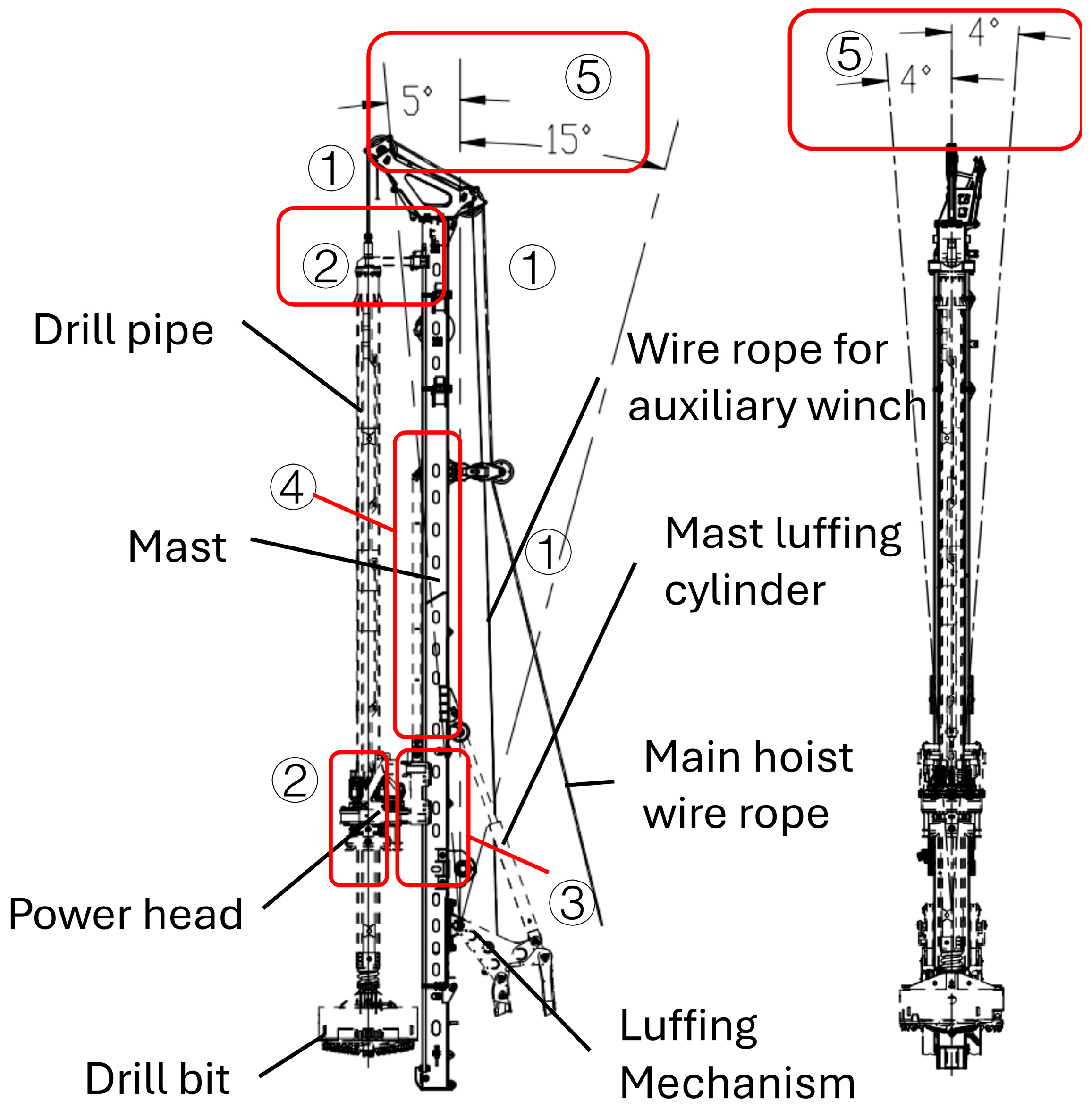
2.1. Introduction to Rotary Drilling Rig

Rotary drilling rigs, as the fundamental equipment for piling works, possess the capabilities of self-propulsion and rotation, enabling them to adapt to various environmental conditions with minimal environmental impact. The working device of a rotary drilling rig primarily consists of a mast, drill pipe, drill bit, power head, and chassis. This study focuses on the mast of a rotary drilling rig, whose structure is shown in Figure 1.

2.2. Classification of Working Conditions

Firstly, the working conditions of rotary drilling rigs are classified into the following seven categories, as shown in

Table 1. Table of working conditions.

Working Condition	Description
Drilling condition B1	The mast is perpendicular to the ground, the drill bit is in contact with the ground, the pressure cylinder applies maximum pressure downward, and the power head drives the drill rod bit to dig downward.
Out-of-hole lifting condition B2	The mast of the rotary drilling rig is perpendicular to the ground, the winch lifts outside the hole, and the self-weight of the power head is borne by the pressure cylinder [20], which does not provide lifting force.
In-hole lifting condition B3	The mast is perpendicular to the ground and the main winch lifts the drill pipe and bit in the hole.
Dumping condition B4	The power head can unload the soil in the drill bit by turning it forward and backward.
Shaking soil condition B5	The rotary drilling rig starts and stops continuously through the winch mechanism, rises and lowers the drill pipe to unload the soil using inertia.
Walking condition B6	With the drill pipe fully retracted and the mast perpendicular to the ground, the rotary drilling rig moves to advance to the next construction position.
Rotating condition B7	The drill pipe is fully recovered, the mast is perpendicular to the ground, and the body is rotated for dumping, shaking, and changing bits.

, including the whole working cycle of rotary drilling rigs, including drilling condition B1, out-of-hole lifting condition B2, in-hole lifting condition B3, dumping condition B4, shaking condition B5, walking condition B6, and rotating condition B7. In this study, we mainly analyze the strength, stiffness, stability, fatigue, and the related calculations.

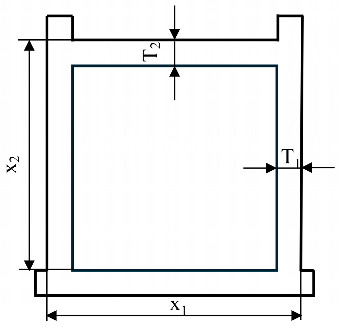
2.3. Optimization Models

In this paper, the minimum cross-section size of the mast is taken as the objective function of optimization, i.e., the principle of minimum weight, and strength, stiffness, stability, and process requirements are taken as the constraints, and a penalty function is used for limitation. By adding a penalty term to the objective function, the constrained optimization problem is transformed into an unconstrained optimization problem. The penalty coefficient is generally set to 12,000 in structural optimization problems. The constrained optimization model of mast weight reduction is shown in Equation (1).

$$\left\{\begin{array}{l}\min A(x)=x_1\times x_2-(x_1-x_3)\times (x_2-x_4)+A_{\mathrm{invariant}};\\ s.t.g_i(x)\le 0 (i=1,2,3,4,5,6,7,8);\\ x={\left[x_1,x_2,x_3,x_4\right]}^T;\end{array}\right.$$

(1)

There are four variables to optimize, i.e., cross-section width x₁, cross-section height x₂, twice the web thickness x₃ = 2 × T₁, and twice the wing thickness x₄ = 2 × T₂. A represents the total cross-sectional area, and A_invariant represents the invariant cross-sectional area, such as the guide rail area, as shown in Figure 2.

2.4. Limitations

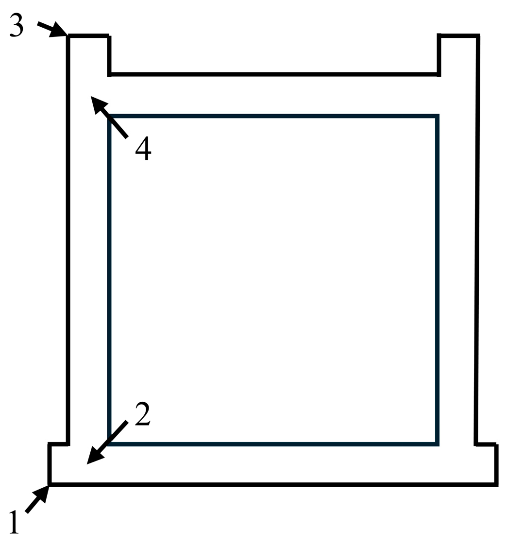
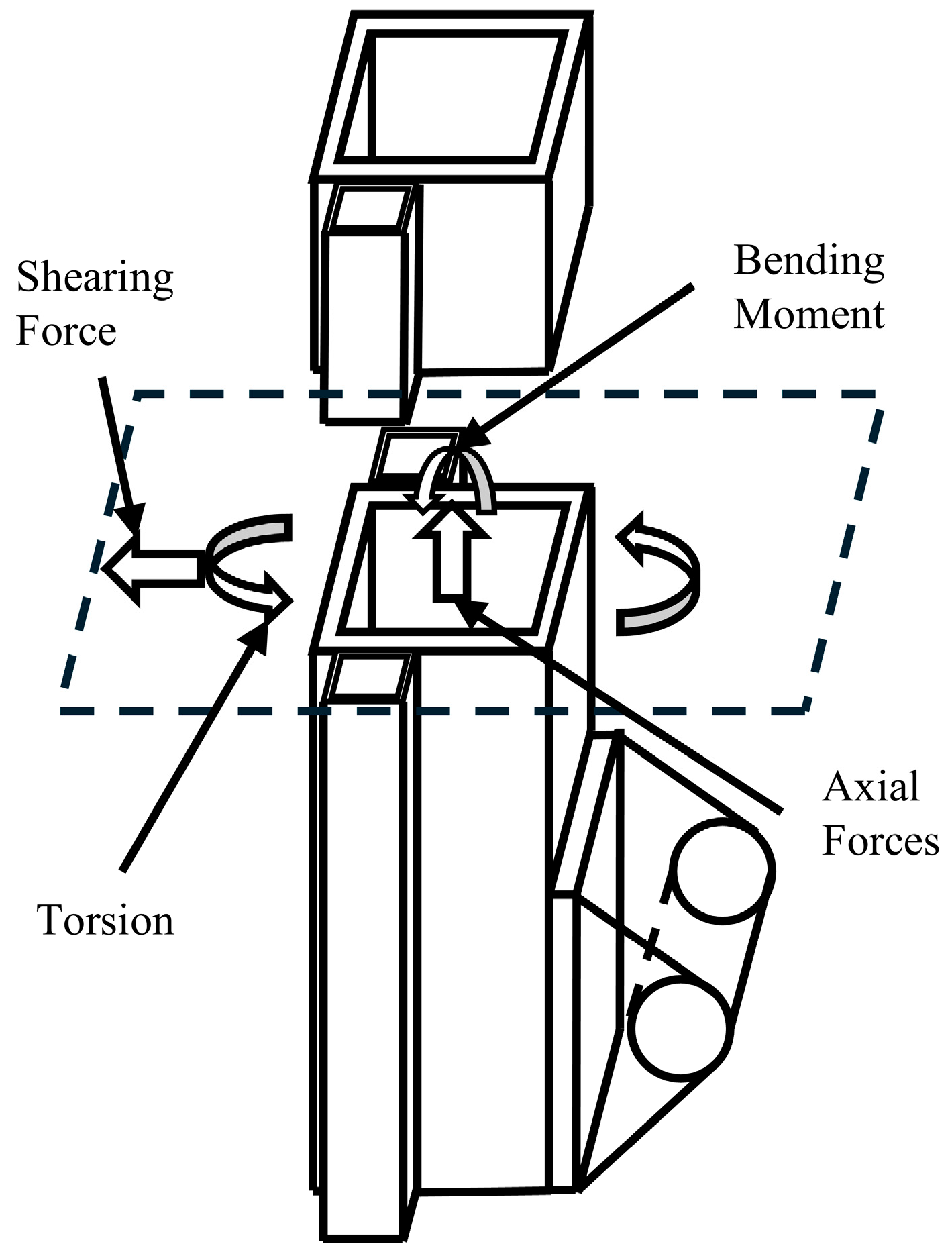
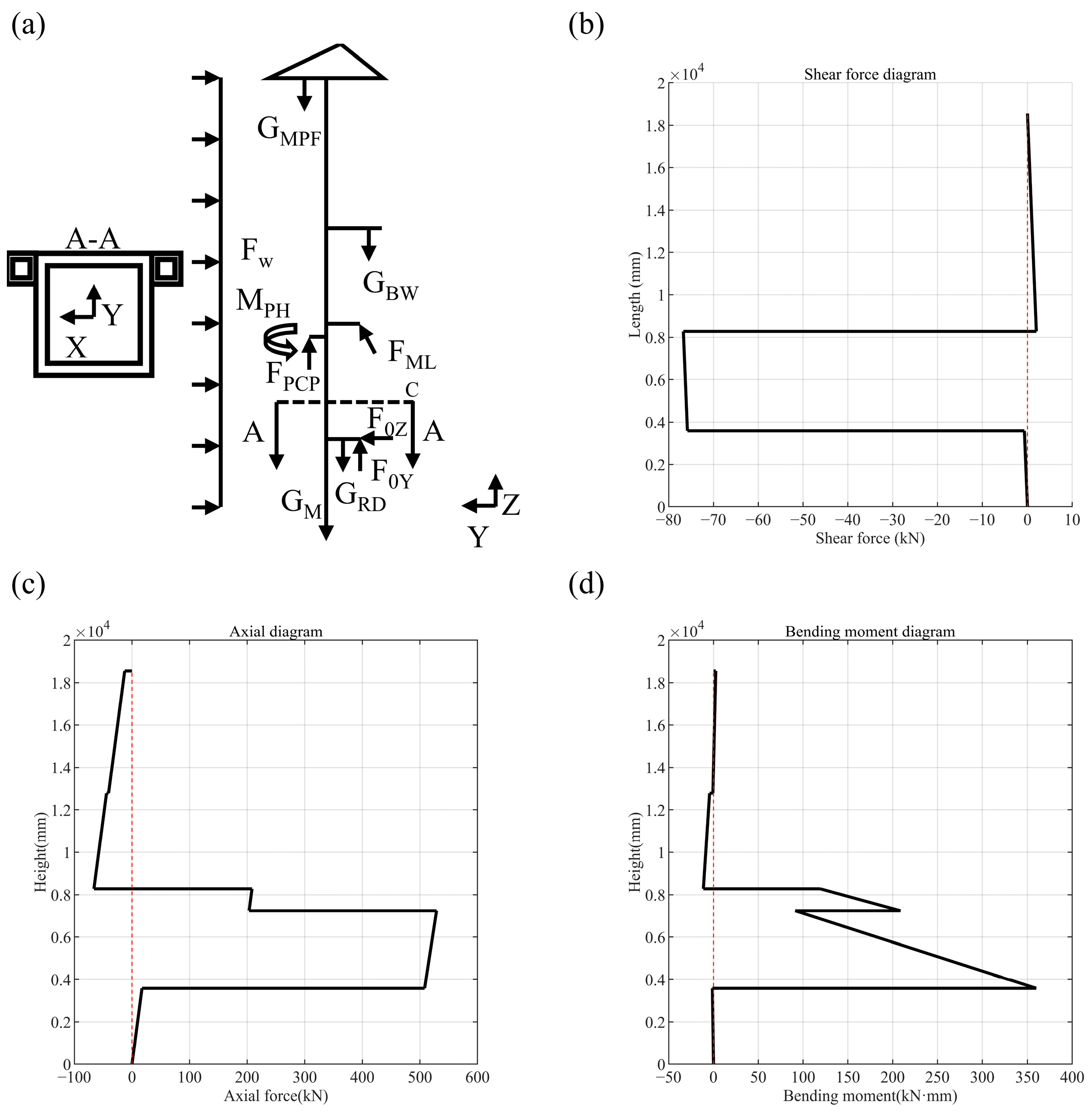
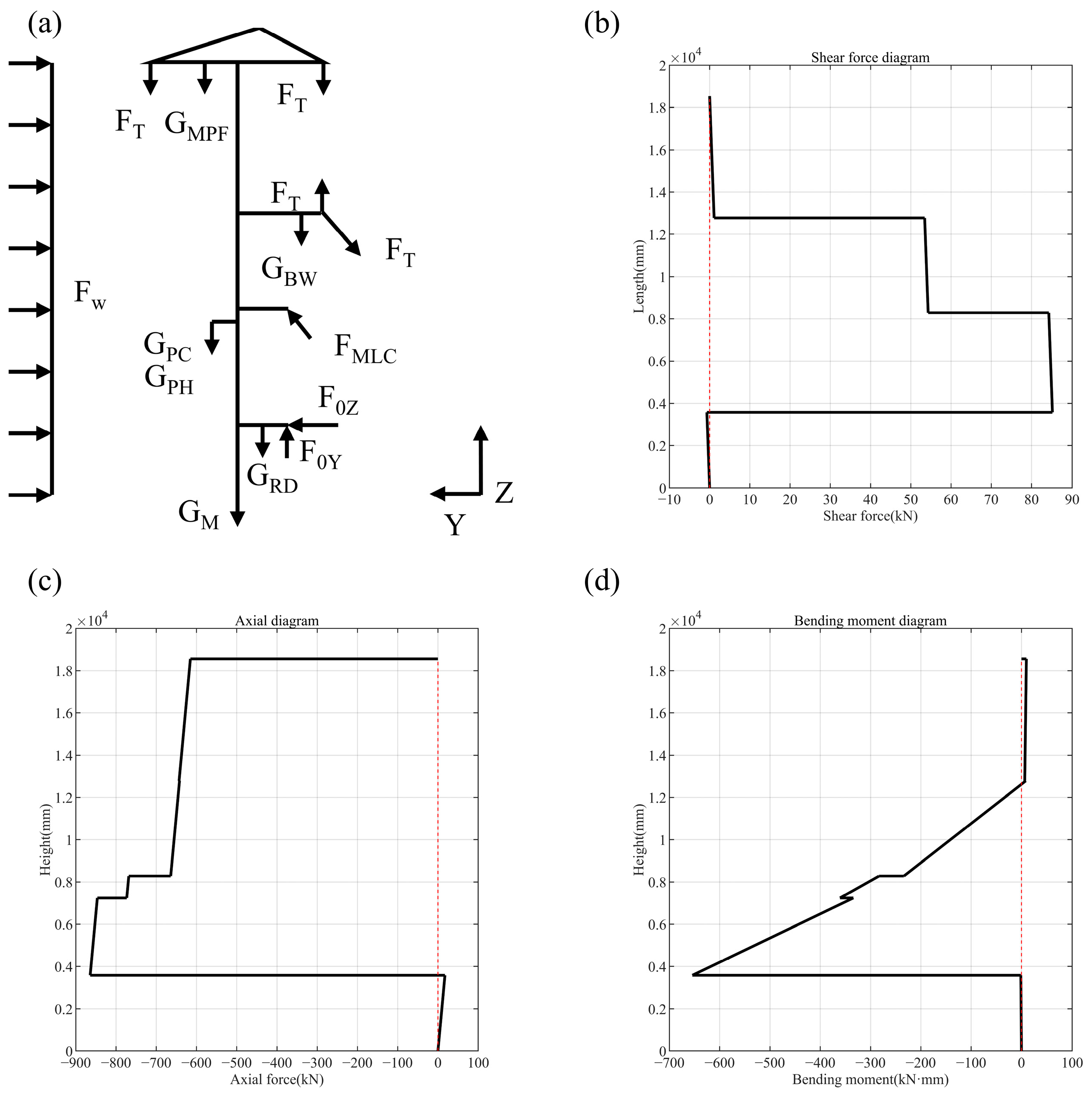
2.4.1. Selection of Hazardous Points for Mast Calibration Section

By calculating the internal force of the mast, the section with the maximum shear force, axial force and bending moment is selected as the dangerous section. According to the stress distribution law of the box section of the mast, points 1, 2, 3 and 4 shown in Figure 3 are selected as the dangerous points for calculation.

2.4.2. Static Strength Checks and Constraints

The static strength analysis of the mast is conducted based on the principle of the most critical working conditions. In the practical application of rotary drilling rigs, the most dangerous working condition is the in-hole lifting condition B3 or the drilling condition B1.

Under drilling conditions, the mast experiences a combination of tensile, bending and torsion deformations [21], as shown in Figure 4.

Specifically, under the B1 condition, points 1 and 3 are only subject to maximum free bending positive stress, which is calculated as shown in Equation (2).

$${\sigma }_0={\displaystyle \frac{N}{A_{\mathrm{j}}}}+{\displaystyle \frac{M_{\mathrm{x}}}{\left(1-(N/N_{Ex})\right)W_{jx}}}+{\displaystyle \frac{M_{\mathrm{y}}}{\left(1-(N/N_{Ey})\right)W_{jy}}}$$

(2)

The points 2 and 4 for B1 are subjected to a combination of the following stresses: free bending positive stress, maximum restrained bending positive stress, restrained torsional positive stress (fan positive stress), bending shear stress as shown in Equation (3), and torsional shear stress as shown in Equation (4). To calculate the constrained bending positive stress and constrained torsion positive stress, the equivalence method is employed, as shown in Equation (5) below.

$${\tau }_{\mathrm{s}}={\displaystyle \frac{F_{\mathrm{shearing}}}{\left(2\times \mathrm{h}\times \delta \right)}}$$

(3)

$${\tau }_{\mathrm{n}}={\displaystyle \frac{T_n}{(2\times A_0\times {\delta }_{\min })}}$$

(4)

$$\sigma =1.15{\sigma }_0$$

(5)

Under in-hole lifting conditions, the mast is subjected to a combination of both tensile (compression) and bending deformations [21]. Points 1 and 3 under the B3 condition are subjected to maximum free bending positive stress only, which is calculated as Equation (2).

Points 2 and 4 under the B3 condition are subjected to free bending positive stresses as in Equation (2), maximum restrained bending positive stresses as in Equation (6), and bending shear stresses as in Equation (3). The constrained bending positive stress is calculated using the equivalent method. The stresses experienced by hazardous points in dangerous working conditions are shown in

Table 2. Stress state.

	B1	B3
Point 1 Point 3	Maximum positive free bending stress
	Unidirectional state of stress at points 1 and 3
Point 2 Point 4	1. Positive free bending stress 2. Maximum positive stress in constrained bending 3. Constrained torsional stress 4. Bending shear stress 5. Torsional shear stress	1. Positive free bending stress 2. Maximum positive bending stress 3. Bending shear stress
	Points 2 and 4 are three-way stress states

.

$$\sigma =1.1{\sigma }_0$$

(6)

For unidirectional positive stresses, the static strength calibration equation is as follows:

$$\sigma \le \left[\sigma \right]$$

(7)

For a spatial stress state, its principal stress can be determined according to the stress tensor. Subsequently, the complex stress state is evaluated and calibrated based on the fourth strength theory.

The stress tensor is as follows:

$$\sigma =\left[\begin{array}{ccc}{\sigma }_{\mathrm{x}}& {\tau }_{xy}& {\tau }_{xz}\\ {\tau }_{yx}& {\sigma }_y& {\tau }_{yz}\\ {\tau }_{zx}& {\tau }_{zy}& {\sigma }_z\end{array}\right]$$

(8)

According to the tensor, its principal stress is as follows:

$${\sigma }_{1,2,3}=\mathrm{eig}(\sigma )$$

(9)

This can be converted to a unidirectional state of stress by the fourth theory of strength, as shown below:

$${\sigma }_{r4}=\sqrt{{\displaystyle \frac{1}{2}}\left[{\left({\sigma }_1-{\sigma }_2\right)}^2+{\left({\sigma }_2-{\sigma }_3\right)}^2+{\left({\sigma }_1-{\sigma }_3\right)}^2\right]}$$

(10)

$${\sigma }_{r4}\le \left[\sigma \right]$$

(11)

Through the above analysis, the stress at the largest point among the four hazardous points is calculated and the static strength constraint is applied to it, and the static strength constraint condition of the mast under working condition B1 is as follows:

$$\mathrm{g}(1)={\sigma }_{B1\max }-\left[\sigma \right]\le 0$$

(12)

The static strength constraints of the mast at operating condition B3 are as follows:

$$g(2)={\sigma }_{B3\max }-\left[\sigma \right]\le 0$$

(13)

2.4.3. Fatigue Calculations and Constraints

Fatigue damage is the primary failure form of engineering machinery structures, which needs to be evaluated based on the load spectrum and SN curve. In this paper, the load spectrum is divided into a complete working cycle, as shown in Figure 5. One cycle consists of the following conditions: drilling condition B1, in-hole lifting condition B3, out-of-hole lifting condition B2, rotating condition B7, dumping condition B4, shaking condition B5, and again rotating condition B7.

Following calibration, the maximum range of the design stress of the structure is less than the range of the ultimate stress, meaning that the fatigue strength of the structure is as follows:

$$\Delta {\sigma }_{S\mathrm{d}}\le \Delta {\sigma }_{Rd}$$

(14)

where is the calculated maximum range of design stresses, as shown below:

$$\Delta {\sigma }_{S\mathrm{d}}=\max \sigma -\min \sigma$$

(15)

where is the ultimate design stress range, as shown below:

$$\Delta {\sigma }_{Rd}={\displaystyle \frac{\Delta {\sigma }_c}{\left({\gamma }_{mf}\sqrt[m]{s_m}\right)}}$$

(16)

With the above calculations, the fatigue strength calibration is transformed into a constraint.

$$g\left(3\right)=\Delta {\sigma }_{S\mathrm{d}}-\Delta {\sigma }_{Rd}\le 0$$

(17)

2.4.4. Stiffness Calculations and Constraints

In engineering, the slenderness ratio is often used for stiffness calibration, the allowable slenderness ratio is [λ], and the calibration method is as follows:

$${\lambda }_{\max }=\sqrt{{\mathrm{l}}_0/r_x}\le \left[\lambda \right]$$

(18)

The stiffness constraints are shown below:

$$g\left(4\right)={\lambda }_{\max }-\left[\lambda \right]\le 0$$

(19)

2.4.5. Stability Calculations and Constraints

The mast is an eccentric compression member and the overall stability is verified according to Equation (20).

$${\displaystyle \frac{N}{\phi A}}+{\displaystyle \frac{M_{\mathrm{x}}}{\left(1-\left(N/N_{Ex}\right)\right)W_x}}+{\displaystyle \frac{M_{\mathrm{y}}}{\left(1-\left(N/N_{E\mathrm{y}}\right)\right)W_y}}\le \left[\sigma \right]$$

(20)

The stability constraints are as follows:

$$g\left(5\right)={\sigma }_{\mathrm{os}}-\left[\sigma \right]\le 0$$

(21)

2.4.6. Process Constraints

According to the force characteristics of the box section of the mast, the width of the wing plate is generally larger than the width of the web plate, and the constraints are given in Equation (22):

$$g(6)=x_2-x_1\le 0$$

(22)

3. Improvement of Salp Swarm Algorithm

3.1. Principles of the Salp Swarm Algorithm

The mathematical model of the SSA [19] divides the population into two categories, the leaders and the followers. The leaders are positioned at the front end of the chain of Salps, while the remaining individuals are the followers. The steps of its original algorithm are shown in Algorithm 1.

Algorithm 1 SSA Flow
1:	Initialization parameters: Population size N and maximum number of iterations L
2:	$\mathrm{Initialize}\mathrm{the}\mathrm{population}.x_j^i=rand(N,D)(u{b}_j-l{b}_j)+l{b}_j$
3:	Selection of food sources F.
4:	for l = 1:L
5:	for i = 1:N
6:	if (i < N/2)
7:	Updating the leader
8:	$x_j^i=\left\{\begin{array}{l}{F}_j+c_1((u{b}_j-l{b}_j)c_2+l{b}_j),c_3\ge 0.5\\ F_j+c_1((u{b}_j-l{b}_j)c_2+l{b}_j),c_3<0.5\end{array}\right.$
9:	else
10:	Update followers
11:	$x_j^i={\displaystyle \frac{1}{2}}(x_j^i+x_j^{i-1})$
12:	end if
13:	end for
14:	Updating of food source F
15:	end while
16:	Output optimal solution

$x_j^i$ is denoted as the position of the jth dimension of the ith slap, N is the population size, D is the dimension, ub_j is the upper bound of the jth dimension variable, and lb_j is the lower bound of the jth dimension variable. F_j is the position of the jth dimension of the food source, c₁ is the convergence factor of the optimization algorithm as shown in the following equation, and c₂ and c₃ are random numbers of [0,1].

$$c_1=2{\exp }^{-{({\displaystyle \frac{4l}{L}})}^2}$$

(23)

where l is the current iteration number and L is the maximum iteration number.

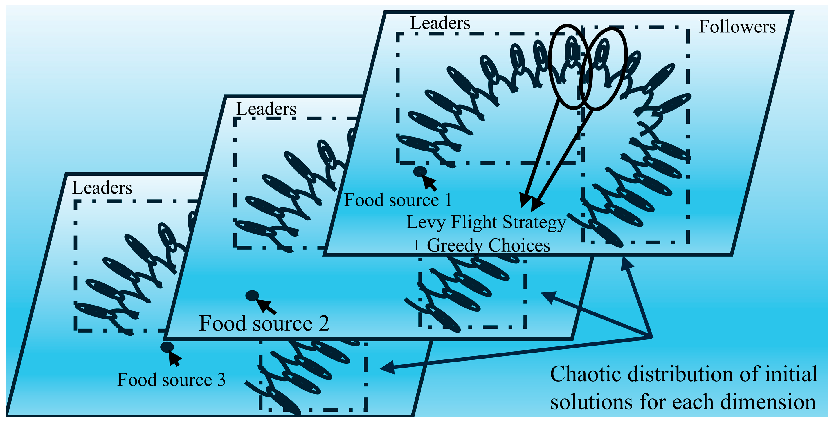
3.2. Improved Salp Swarm Algorithm

Optimization problems are subject to different types of constraints in both science and engineering fields [22]. For structural optimization problems in the engineering field, there are some specific requirements that need to be considered, such as the welded parts of the box section. The plate widths are usually integers, while plate thicknesses are usually standard plate thicknesses, most of which are even numbered. Additionally, the widths of the wing plates are larger than those of the web plates, etc. Imposing these practical design constraints accurately is a challenge for traditional swarm optimization algorithms. To address these challenges, this paper proposes the Improved Salp Swarm Algorithm (ISSA) as a suitable optimization method for determining the welded cross-section sizes. The ISSA enhances iterative ability, improves the quality of the solution, and maintains robust optimization performance in structured problems.

3.2.1. Algorithmic Multidimensional Settings

The core logic of the algorithm is to update the positions of the independent variables x₁ and x₂ accordingly, while x₃ and x₄ are used to select from the standard plate thickness data T to obtain a solution set that satisfies the procurement requirements. The plate thickness data T value is shown in Equation (24).

$$T=[T_1,\cdots \cdots T_z]$$

(24)

The multidimensional setting strategy of the algorithm is to make permutations and combinations from the given plate thickness dataset. For example, when T = [4,5,6,8,10], the dimensionality of the algorithm is N = size(T) × size(T) = 25. Each dimension corresponds to a kind of x₃ and x₄ solution set, as shown in Figure 6. If not stated separately, the following policy updates are operations of the optimization variables x₁ and x₂.

3.2.2. Population Initialization

The traditional Salp Swarm Algorithm (SSA) utilizes a randomly generated initial population, which can lead to an uneven distribution of the initial solutions within the search space. To address this issue, chaos-based techniques have been widely employed to enhance the performance of meta-inspired algorithms [12]. Among the commonly used chaotic mappings, Tent mapping has been shown to provide a more uniform distribution of initial solutions compared to Logistic mapping [23]. In this paper, Tent chaotic mapping is used for pseudo-random generation of initial solutions, which can make the distribution of initialized populations in the definition domain more uniform and improve the algorithm’s ability to traverse globally between the upper and lower bounds of the optimization variables.

In this paper, the optimization variables are separately distributed chaotically for each dimension separately as shown in Equation (26).

$$y_j^{i+1}=\left\{\begin{array}{c}{y}_j^i/0.499,0\le y_j^i\le 0.499\\ (1-y_j^i)/(1-0.499),0.499<y_j^i\le 1\end{array}\right.$$

(25)

$$x{[n]}_j^i=lb+(ub-lb)\times y_j^i$$

(26)

where x[n${]}_j^i$ denotes the nth dimension, the ith Salp and the jth variable; lb and ub are the upper and lower bounds of the optimization variables.

Subsequently, the fitness of the initial solution is computed and selected for each dimension using the food source F[n].

3.2.3. Leader Renewal

In the Salp Swarm Algorithm, the position of the food source is the target position of all Salp individuals, i.e., the global optimal solution during the search process, which influences the leader position update, and the number of leaders is taken to be half of the number of populations. The leader of each dimension performs an update operation for the food source of each dimension as in Equation (28).

$$c_1={\exp }^{(-{(4l/L)}^2)}$$

(27)

$$x{[n]}_j^i=round\left\{\begin{array}{c}(F{[n]}_j+c_1((u{b}_j-l{b}_j)c_2+l{b}_j)),c_3\ge 0.5\\ (F{[n]}_j-c_1((u{b}_j-l{b}_j)c_2+l{b}_j)),c_3<0.5\end{array}\right.$$

(28)

where F[n]_j is the location of the jth variable of the n-dimensional food source. c₁ is the convergence factor in the algorithm, which plays the role of balancing global exploration and local exploitation and is the most important parameter. c₂ and c₃ are [0,1] random numbers used to enhance randomness and increase diversity. l is the current number of iterations. L is the maximum number of iterations.

3.2.4. Follower Updates

The position of the ith Salp follower in the traditional Salp Algorithm is only related to itself and the i – 1th Salp. If the leader Salp converges to a local optimum, the follower Salp will also be trapped in the same local optimal solution, preventing the global optimal solution from being obtained. In this paper, it is improved by using Levy flights and greedy selection to make the algorithm more likely to jump out of the local optimum. The strategy adopted is shown below.

For the problem that the algorithm easily falls into the local optimal solution, the strategy of introducing Levy flight perturbation as a random wandering process can make the algorithm change randomly between long and short distances, and it can realize the long-time and short-distance back-and-forth search interspersed with the occasional long-distance search [24]. It can satisfy both small-scale fine searches and large-scale global searches, which can realize the diversification of the search domain and enhance the global search capability.

There are three alternatives for the follower. The first is the previous leader or the follower itself as in Equation (29), the second is that the former imposes a Levy flight perturbation as in Equation (30), and the third is that the follower follows the previous individual and their displacements conform to Newton’s Laws of Motion as in Equation (31).

$$p[n]=\left\{\begin{array}{cc}x{[n]}_j^i,\hfill & c_4\ge 0.5\hfill \\ x{[n]}_j^{i-1},\hfill & c_4<0.5\hfill \end{array}\right.$$

(29)

$$pp[n]=\left\{\begin{array}{l}p[n]+round(5\times s),c_5\le 0.5\\ p[n]-round(5\times s),c_5>0.5\end{array}\right.$$

(30)

$$ppp[n]={\displaystyle \frac{1}{2}}(x{[n]}_j^i+x{[n]}_j^{i-1})$$

(31)

where c₄ and c₅ are random numbers of [0,1] and s is the Levy flight step as shown in Equation (32).

$$s={\displaystyle \frac{\mu }{{\left|\nu \right|}^{1/\beta }}}$$

(32)

where ${\sigma }_{\mu }$ and ${\sigma }_{\nu }$ are obtained from Equation (33), as shown below:

$$\left\{\begin{array}{l}{\sigma }_{\mu }={\left\{{\displaystyle \frac{\Gamma (1+\beta )\sin (\pi \beta /2)}{\Gamma [(1+\beta )/2]\beta 2^{(\beta -1)/2}}}\right\}}^{1/\beta }\\ {\sigma }_{\nu }=1\end{array}\right.$$

(33)

The value of the parameter ranges from 0 to 2 and is taken as = 1.5 in this paper.

In this paper, the greedy selection method, which is a strategy that always selects the option with the best immediate reward or fitness, is used to decide the position of the update follower, i.e., the one with the best fitness among the alternative options is selected, as shown in Equation (34).

$$x{[n]}_j^i=\left\{\begin{array}{c}p[n],f[p[n]]<f[pp[n]]\&\&f[p[n]]<f[ppp[n]]\hfill \\ pp[n],f[pp[n]]<f[p[n]]\&\&f[pp[n]]<f[ppp[n]]\hfill \\ ppp[n],f[ppp[n]]<f[p[n]]\&\&f[ppp[n]]<f[pp[n]]\hfill \end{array}\right.$$

(34)

Under this strategy, the solutions will be diverse and the algorithm is more likely to jump out of the local optimum. The pseudo-code of the algorithm is shown in Algorithm 2.

Algorithm 2 Pseudo-Code of Proposed ISSA
1:	Initialization
2:	Define the population size M, algorithm dimension N, maximum iteration times L.
3:	The variables for the initial population in each dimension were chaotically distributed and rounded (The following variables are the variables x1 and x2, unless otherwise specified).
4:	Find the optimal initial values for each dimension and select for each dimension food source.
5:	for l = 1:L
6:	for n = 1:N
7:	for m = 1:M
8:	if i ≤ M/2 update leader position
9:	Leaders in each dimension move toward the food source in each dimension
10:	else
11:	Updating individual variables of followers in each dimension using Levy flight perturbation and greedy selection strategy
12:	end if
13:	end for
14:	Calculating adaptation, updating the food source for each dimension and recording the global optimal food source
15:	end for
16:	end for
17:	Update the optimal solution in all dimensions
18:	Finish

4. Experiments

4.1. Parameterization

In this section, the mast of a certain type of rotary drilling rig is selected as an example to carry out the study, the size of the mast is 600 × 600 mm, the thickness of the web plate and the thickness of the wing plate is 10 mm, and the model parameters are shown in

Table 3. Model parameter list.

Parameters	Numerical Value
Mast deadweight	GM = 70.71 kN
Self-weight of rotary disk	GRD = 5.13 kN
Back wheel deadweight	GBK = 2.76 kN
Main pulley frame deadweight	GMPF = 9.89 kN
Pressure cylinder deadweight	GPC = 6.79 kN
Pressure cylinder pressurization	FPCP = 210 kN
Pressure cylinder lifting force	FT1 = 210 kN
The main hoist lifting force	FT = 190 kN
Power head torque	MPH = 210 kN·m
Self-weight of power head	GPH = 50.51 kN

below.

The mast’s strength, stiffness, and stability checks were carried out as previously described and an optimization model with the objective function of minimizing weight was established. The range of variation of the independent variables was set as lb = [100,100,8,8], ub = [600,600,20,20], and the dataset of the commonly used standard thick steel plates below 10 mm was [4,5,6,8,10]. The initial parameters of the algorithm were set with the total number of iterations as L = 100 and the size of the population as M = 100. For its constraints, a penalty function was used for constraints and it was verified that a penalty function factor of 12,000 is more suitable for this problem. In order to verify the feasibility of this paper, traditional algorithms such as the Whale Optimization Algorithm (WOA) [25], SSA [19], and Grey Wolf Optimizer (GWO) [26] were also used and the same parameters were set for the traditional structure optimization. The optimization process was implemented on the platform MATLAB R2021a.

4.2. Constraints

In drilling conditions, the main hoist is not operational, and the pressure cylinder is pressurized downward with the maximum pressure. The power head provides torque for the drill pipe, and the weight of the drill pipe, the drill bit and the power head is borne by the ground. The mast is constrained by the mast’s deadweight G_M, the rotary disk’s deadweight G_RD, the back wheel’s deadweight G_BW, the main pulley frame G_MPF, the pressure cylinder pressurization F_PCP, and the wind load F_w. The mast has two constraints: the fixed hinge constraint of the rotary disk and the movable hinge constraint of the mast luffing cylinder. The force diagram is shown in Figure 7a. The equilibrium equations were solved, and the support reaction forces at the constraints were calculated as F_OY = −75.13 kN, F_OZ = −484.15 kN and F_MLC = 285.56 kN. We calculated the internal forces based on the external forces and created a shear force diagram, axial force diagram and bending moment diagram, as shown in Figure 7b–d.

The lifting condition in the hole, the winch lifting with full power and the force diagram are shown in Figure 8a. The mast was subjected to the self-weight of the mast G_M, the self-weight of the rotary disk G_RD, the self-weight of the back wheel G_BW, the main pulley frame G_MPF, pressure cylinder deadweight G_PC = 6.79 kN, the self-weight of power head G_PH, the main hoist lifting force F_T and the wind load F_w for the same reason as in the column balance equation, and we solved its cross-section internal force, creating an internal force diagram, as shown in Figure 8b–d.

In addition to the two working conditions described above, the remaining five working conditions are similar in nature but are not considered hazardous. Therefore, the calculation process for these conditions is omitted here, as they do not require static strength checks. According to the internal force diagram for each working condition, it is found that the internal force of the rotary disk for the mast is the largest, which represents the critical section of the entire mast. Consequently, the static strength of this section was evaluated. The mast material is Q355 steel, and the constraints for B1 and B3 working conditions are written according to Equations (12) and (13).

B3 working condition:

$$g\left(1\right)={\sigma }_{B1\max }-323\le 0$$

(35)

B1 working condition:

$$g\left(2\right)={\sigma }_{B3\max }-323\le 0$$

(36)

According to Equation (17), the fatigue constraints are as follows:

$$g\left(3\right)=\Delta {\sigma }_{S\mathrm{d}}-243\le 0$$

(37)

The stiffness constraint of the mast according to Equation (19) is as follows:

$$g\left(4\right)={\lambda }_{\max }-180\le 0$$

(38)

According to Equation (21), the stability constraints are as follows:

$$g\left(5\right)={\sigma }_{\mathrm{os}}-323\le 0$$

(39)

According to the force characteristics of the box section of the mast, the width of the wing plate is generally larger than the width of the web plate, as shown in Equation (40):

$$g(6)=x_2-x_1\le 0$$

(40)

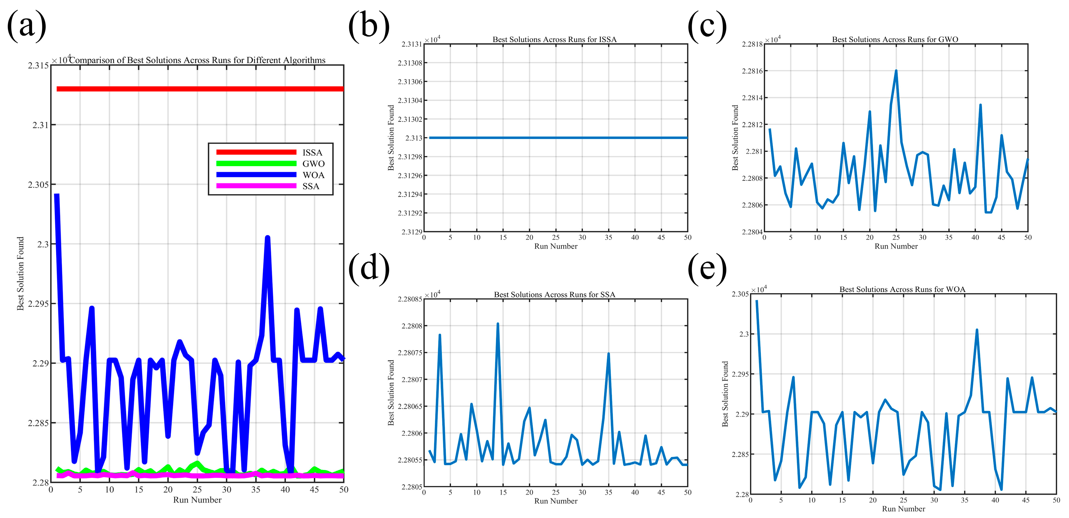
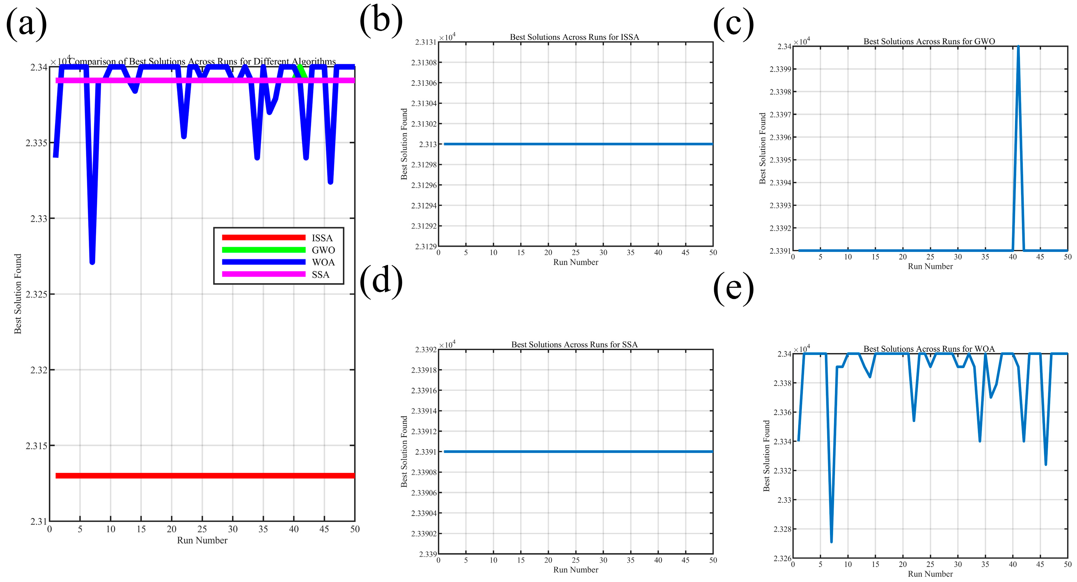
4.3. Comparison and Analysis of Optimization Results

The iteration curves of each algorithm are shown in Figure 9, which shows that the initial solution for ISSA has higher adaptability and the iteration process is smooth, proving the effectiveness of the improvement in this paper.

The comparison results of the optimization algorithms are shown in

Table 4. Empirical results.

	ISSA	GWO	SSA	WOA
x1	591	600	600	600
x2	591	600	600	600
x3	10	10.34	10.42	11.20
x4	20	18.66	18.58	17.87
g1	−89.33	−85.50	−85.06	−81.35
g2	−123.10	−121.20	−121.06	−119.88
g3	−60.77	−57.36	−56.87	−51.95
g4	−83.82	−84.55	−84.46	−83.63
g5	0	0	0	0
g6	−0.33	0	0	0
Degree of adaptation	23,130	22,808.40	22,805.90	22,842.80

below.

From the data presented in the above table, it can be concluded that the performance of the algorithms does not exhibit significant differences, with the ISSA appearing to be at a disadvantage. However, from the perspective of practical feasibility, the algorithm proposed in this study is superior. For the optimization variables x₁ and x₂, where the integer or fractional difference is negligible, but the plate thickness is either standard or not, the manufacturer cannot produce any plate thickness, such as a web thickness of 5.1686 mm or the wing thickness of 9.32925 mm for the GWO results. In conventional ground structure optimization, plate thicknesses can only be rounded upwards to integer plate thicknesses, followed by the selection of applicable standard plate thicknesses. This series of operations inevitably alters the adaptability of the algorithm, which leads to an increase in the objective function and ultimately prevents the attainment of the optimal solution. As shown in

Table 5. Results of standard plate thickness.

	ISSA	GWO	SSA	WOA
x1	591	600	600	600
x2	591	600	600	600
x3	10	11	11	12
x4	20	19	19	18
Degree of adaptation	23,130	23,391	23,391	23,384

below, the algorithm proposed in this study can effectively address this problem.

The plate thickness of the above traditional algorithm, following upward rounding, may still be non-standard, e.g., the web thickness of 5.5 mm for GWO represents a non-standard plate thickness, necessitating further upward rounding, which leads to a continued increase in the value of the objective function. It can be concluded that the solution of ISSA is both reasonable and optimal.

In addition, to assess the stability of the algorithms, a comparison was conducted among the four algorithms after 50 iterations, as shown in Figure 10a–e. After comparison, it was proposed that the algorithm in this paper is highly robust. Then, the thickeness was rounded upward and compared again, as shown in Figure 11a–e.

The figure concludes that the ISSA proposed in this paper can converge to the optimal solution stably and reliably. In contrast, the traditional algorithms exhibit poor convergence stability and inferior solution quality.

5. Conclusions

This study addresses the issues of high power consumption and poor economic efficiency in rotary drilling rigs by proposing the use of the Improved Salp Swarm Algorithm (ISSA) for the lightweight design of the mast. The objective function is set to minimize the box section size of the mast, with strength, stiffness, stability, and fatigue as constraints, which are optimized using the ISSA.

The results show that the cross-section size changes from 600 × 600 to 591 × 591, and the thickness of the web plate is reduced from a 10 mm thick steel plate to a 5 mm thick steel plate, resulting in a significant 20% weight reduction. Compared to the traditional optimization algorithm, it can be concluded that the improved SSA demonstrated high solution quality, exhibiting excellent solving ability for the structural optimization of box section size and plate thickness. The improved SSA was able to reasonably solve the optimal solution with a notable effect, providing a valuable reference for future optimization design.

Future work will focus on integrating machine learning with the Improved Salp Swarm Algorithm to further enhance the accuracy of the optimization model. By leveraging historical data, the machine learning model will predict the carrying capacity of the rotary drilling rig mast and use it as a constraint, thereby improving the model’s precision and yielding more reliable results. This approach will lay the foundation for the application of digital twin technology, making structural optimization more forward-looking and data-driven.

References

1. Savković, M.M.; Bulatović, R.R.; Gašić, M.M.; Pavlović, G.V.; Stepanović, A.Z. Optimization of the box section of the main girder of the single-girder bridge crane by applying biologically inspired algorithms. Eng. Struct. 2017, 148, 452–465. [Google Scholar] [CrossRef]
2. Cheng, B.; Qian, Q.; Sun, H. Steel truss bridges with welded box-section members and bowknot integral joints, Part II: Minimum weight optimization. J. Constr. Steel Res. 2013, 80, 475–482. [Google Scholar] [CrossRef]
3. Qi, Q.; Yu, Y.; Dong, Q.; Xu, G.; Xin, Y. Lightweight and green design of general bridge crane structure based on multi-specular reflection algorithm. Adv. Mech. Eng. 2021, 13, 16878140211051220. [Google Scholar] [CrossRef]
4. Pavlović, G.V.; Zdravković, N.B.; Savković, M.M.; Bulatović, R.R.; Marković, G.Đ. Light-weight design of an overhead crane’s girder with a non-symmetric box cross-section. Proc. Inst. Mech. Eng. Part C J. Mech. Eng. Sci. 2024, 238, 666–676. [Google Scholar] [CrossRef]
5. Cuong-Le, T.; Minh, H.-L.; Khatir, S.; Wahab, M.A.; Tran, M.T.; Mirjalili, S. A novel version of Cuckoo search algorithm for solving optimization problems. Expert Syst. Appl. 2021, 186, 115669. [Google Scholar] [CrossRef]
6. Kaveh, A.; Talatahari, S. An improved ant colony optimization for constrained engineering design problems. Eng. Comput. 2010, 27, 155–182. [Google Scholar] [CrossRef]
7. Pavlović, G.; Savković, M. Analysis and optimization of the main girder of the bridge crane with an asymmetric box cross-section. Sci. Tech. Rev. 2022, 72, 3–11. [Google Scholar] [CrossRef]
8. Hijjawi, M.; Alshinwan, M.; Khashan, O.A.; Alshdaifat, M.; Almanaseer, W.; Alomoush, W.; Garg, H.; Abualigah, L. Accelerated arithmetic optimization algorithm by cuckoo search for solving engineering design problems. Processes 2023, 11, 1380. [Google Scholar] [CrossRef]
9. Abdel-Basset, M.; Wang, G.-G.; Sangaiah, A.K.; Rushdy, E. Krill herd algorithm based on cuckoo search for solving engineering optimization problems. Multimed. Tools Appl. 2019, 78, 3861–3884. [Google Scholar] [CrossRef]
10. Askarzadeh, A. A novel metaheuristic method for solving constrained engineering optimization problems: Crow search algorithm. Comput. Struct. 2016, 169, 1–12. [Google Scholar] [CrossRef]
11. Salgotra, R.; Singh, U.; Singh, S.; Singh, G.; Mittal, N. Self-adaptive salp swarm algorithm for engineering optimization problems. Appl. Math. Model. 2021, 89, 188–207. [Google Scholar] [CrossRef]
12. Sayed, G.I.; Khoriba, G.; Haggag, M.H. A novel chaotic salp swarm algorithm for global optimization and feature selection. Appl. Intell. 2018, 48, 3462–3481. [Google Scholar] [CrossRef]
13. Al-Betar, M.A.; Kassaymeh, S.; Makhadmeh, S.N.; Fraihat, S.; Abdullah, S. Feedforward neural network-based augmented salp swarm optimizer for accurate software development cost forecasting. Appl. Soft Comput. 2023, 149, 111008. [Google Scholar] [CrossRef]
14. Zhang, D.; Sun, D.; Zhang, L. DV-Hop localization algorithm based on simulated annealing and optimization of salp swarm. Transducer Microsyst. Technol. 2024, 43, 125–129. [Google Scholar]
15. Tang, X.; Cheng, Y.; Pan, S. Look-ahead distance optimization method for pure pursuit control based on time delay compensation. J. Chin. Inert. Technol. 2023, 31, 876–882. [Google Scholar]
16. Altay, O.; Cetindemir, O.; Aydogdu, I. Size optimization of planar truss systems using the modified salp swarm algorithm. Eng. Optim. 2024, 56, 469–485. [Google Scholar] [CrossRef]
17. Hichri, A.; Hajji, M.; Mansouri, M.; Nounou, H.; Bouzrara, K. Supervised machine learning-based salp swarm algorithm for fault diagnosis of photovoltaic systems. J. Eng. Appl. Sci. 2024, 71, 12. [Google Scholar] [CrossRef]
18. Barhoush, M.; Abed-alguni, B.H.; Al-qudah, N.E.A. Improved discrete salp swarm algorithm using exploration and exploitation techniques for feature selection in intrusion detection systems. J. Supercomput. 2023, 79, 21265–21309. [Google Scholar] [CrossRef]
19. Mirjalili, S.; Gandomi, A.H.; Mirjalili, S.Z.; Saremi, S.; Faris, H.; Mirjalili, S.M. Salp Swarm Algorithm: A bio-inspired optimizer for engineering design problems. Adv. Eng. Softw. 2017, 114, 163–191. [Google Scholar] [CrossRef]
20. Kang, H.; He, Q.; Xie, Y. Mechanics analysis of rotary drilling rig under drilling-bucket-lifting conditions. Eng. Mech. 2010, 27, 214–218. [Google Scholar]
21. Kang, H. Study on Mechanical Properties and Optimization of Working Device of Rotary Drilling Rig; Central South University: Changsha, China, 2013. [Google Scholar]
22. Mohamed, A.W. A novel differential evolution algorithm for solving constrained engineering optimization problems. J. Intell. Manuf. 2017, 29, 659–692. [Google Scholar] [CrossRef]
23. Dan, L.; Qiang, H.; Li, J. Chaotic optimization algorithm based on Tent map. Control. Decis. 2005, 20, 179–182. [Google Scholar]
24. Lu, X.-L.; He, G. QPSO algorithm based on Lévy flight and its application in fuzzy portfolio. Appl. Soft Comput. 2021, 99, 106894. [Google Scholar] [CrossRef]
25. Mirjalili, S.; Lewis, A. The Whale Optimization Algorithm. Adv. Eng. Softw. 2016, 95, 51–67. [Google Scholar] [CrossRef]
26. Mirjalili, S.; Mirjalili, S.M.; Lewis, A. Grey Wolf Optimizer. Adv. Eng. Softw. 2014, 69, 46–61. [Google Scholar] [CrossRef]
Figure 1. Rotary drilling rig. (1) Guidance and load-bearing of the main and auxiliary wire ropes. (2) Guidance of the drill pipe. (3) Guidance and load-bearing of the power head. (4) Pressurization and lifting of the power head. (5) Pose adjustment.
Applsci 14 10040 g001
Figure 2. Box section parameters for rotary drilling rigs.
Applsci 14 10040 g002
Figure 3. Location of cross-section dangerous points.
Applsci 14 10040 g003
Figure 4. Diagram of the internal forces in section of the mast.
Applsci 14 10040 g004
Figure 5. Typical work cycle of a rotary drilling rig.
Applsci 14 10040 g005
Figure 6. Schematic diagram of the principle of the ISSA.
Applsci 14 10040 g006
Figure 7. Force diagram for drilling conditions. (a) Mechanical model for drilling conditions; (b) Shear force diagram for drilling conditions; (c) Axial force diagram for drilling conditions; (d) Bending moment diagram for drilling conditions. (The red line indicates the zero position).
Applsci 14 10040 g007
Figure 8. Force diagram for in-hole lifting condition. (a) Mechanical model for extreme lifting conditions; (b) Shear force diagram for extreme lifting conditions; (c) Axial force diagram for extreme lifting conditions; (d) Bending moment diagram for extreme lifting conditions. (The red line indicates the zero position).
Applsci 14 10040 g008
Figure 9. Algorithm iteration diagram. (a) Iteration graph of ISSA; (b) Iteration graph of GWO; (c) Iteration graph of SSA; (d) Iteration graph of WOA; (e) Comparison of iteration processes for each algorithm.
Applsci 14 10040 g009
Figure 10. Algorithm stability comparison. (a) Comparison of 50 iterations for each algorithm; (b) Results of 50 iterations for ISSA; (c) Results of 50 iterations for GWO; (d) Results of 50 iterations for SSA; (e) Results of 50 iterations for WOA.
Applsci 14 10040 g010
Figure 11. Comparison of algorithms after rounding. (a) Comparison of algorithms after rounding upward; (b) Results of ISSA after rounding upward; (c) Results of GWO after rounding upward; (d) Results of SSA after rounding upward; (e) Results of WOA after rounding upward.
Applsci 14 10040 g011