A Novel Approach to Transient Fourier Analysis for Electrical Engineering Applications

Abstract

This paper presents a detailed investigation into the application of transient Fourier analysis in select electrical engineering contexts. Two novel approaches for addressing transient analysis are introduced. The first approach combines the Fourier series with the Laplace–Carson ($\mathcal{L}\text{-}C$) transform in the complex domain, utilizing complex time vectors to streamline the computation of the original function. The inverse transformation back into the time domain is achieved using the Cauchy-Heaviside ($C\text{-}\mathcal{H}$) method. The second approach applies the Fourier transform ($\mathcal{F}\text{-}{\rm T}$) for the transient analysis of a power converter circuit with both passive and active loads. The method of complex conjugate amplitudes is employed for steady-state analysis. Both contributions represent innovative approaches within this study. The process begins with Fourier series expansions and the computation of Fourier coefficients, followed by solving the system’s steady-state and transient responses. The transient states are then confirmed using the Fourier transform. To validate these findings, the analytical results are verified through simulations conducted in the Matlab/Simulink R2023b environment.

1. Introduction

The transient analysis of dynamic systems plays a crucial role in understanding system behavior and is equally important as steady-state analysis. While steady-state analysis focuses on the equilibrium conditions of a system, transient analysis examines the rapid variations that occur within the system over time [1,2,3,4,5]. These rapid changes, however, cannot happen instantaneously due to the energy exchange processes involved, typically between the magnetic fields in inductors and the electric fields in capacitors. If energy were to change instantaneously, it would imply infinite power, which contradicts the laws of physical reality [1,2].

To analyze transient phenomena, several methods have been developed, including classical techniques, the Cauchy-Heaviside ($C\text{-}\mathcal{H}$) operational method, the Fourier transform, and the Laplace transform. The ($C\text{-}\mathcal{H}$) operational method, sometimes referred to as the symbolic method, simplifies the analysis by replacing derivatives with symbolic operators (such as s or p) [2].

Transient processes are particularly significant in power electronic systems (PES), as they occur over short time intervals and are characterized by substantial energy exchange [2]. The Fourier series has wide-ranging applications across various fields in the natural sciences and mathematics [3]. In [6], two novel methods for analyzing circuits with semiconductor elements are introduced: the Φ-function method and the complex conjugate amplitude method. The work [6] does not deal with or investigate nonlinear functions, nor does it address the Fourier transform. In our case, the function under study does not necessarily have to be analytic, or even strictly periodic, i.e., it does not have to meet the Dirichlet conditions, except in the cases of Fourier analysis, as mentioned in the conclusion of our paper.

This paper introduces two novel and effective approaches for transient analysis within the field of electrical engineering (EE):

• A method that employs the Laplace–Carson (L-C) transform in the complex domain, significantly simplifying the computation of the original function.
• The use of Fourier transform techniques to analyze transient states, particularly in electrical and electronic applications.

This study covers three major aspects of Fourier analysis: Fourier series/expansions, application within the orthonormal complex domain, and Fourier integral transforms. The paper is structured as follows:

• Introduction.
• Fourier Analysis in Time and Complex Domains, including the method of complex conjugate amplitudes and transient analysis under non-harmonic excitation.
• Transient Analysis of Power Electronic Systems (PESs) using Fourier integral transforms, illustrated with two application examples from the EE field.
• Validation of System States using Matlab/Simulink.
• Discussion and Conclusion.

2. Fourier Analysis in the Time and Complex Domains

Fourier series, in many respects, offers a broader scope of applicability compared to the more familiar Taylor series from calculus. This is because the Fourier series can represent a wide range of discontinuous periodic functions, which often arise in real-world applications, whereas such functions may not always have a valid Taylor series expansion [4]. As an illustrative example, we can consider the pulse waveforms commonly generated by power electronic systems, as shown in Figure 1 [5,6,7].

The Fourier series is expressed by the following relation [1,2,3,4],

$$u\left(t\right)=\sum _{\nu =1}^{\mathrm{\infty }}\left[A_{\nu }\cos \nu \omega t+B_{\nu }\sin \nu \omega t\right],$$

(1)

where $A_{\nu },\mathrm{a}\mathrm{n}\mathrm{d} B_{\nu }$ are amplitudes of harmonic functions, which are the functions of the Fourier coefficients $a_{\nu },\mathrm{a}\mathrm{n}\mathrm{d} b_{\nu }$, multiplied by the maximal value $U_m$ or [8]

$$u\left(t\right)=\sum _{\nu =1}^{\mathrm{\infty }}{C}_{\nu }\cos (\nu \omega t+{\delta }_{\nu }),$$

(1a)

where

$$C_{\nu }=\sqrt{A_{\nu }^2+B_{\nu }^2};\hspace{1em}\tan {\delta }_{\nu }={\displaystyle \frac{B_{\nu }}{A_{\nu }}}.$$

(1b)

Current waveform under linear R-L load can be derived using complex conjugate amplitudes [6] applied on Equation (1a) for steady-state and zero initial conditions

$$\begin{gathered} i\left(t\right)={\sum _{\nu =0}^{\mathrm{\infty }}{\displaystyle \frac{C_{\nu }\cos (\nu \omega t+{\delta }_{\nu })}{R+dL}}⌋}_{d\equiv j\nu \omega }\leftrightarrow \\ \mathit{i}\left(t\right)={\displaystyle \frac{1}{2}}\sum _{\nu =0}^{\mathrm{\infty }}{C}_{\mathrm{n}}{\displaystyle \frac{e^{j\left(\nu \omega t+{\delta }_{\nu }\right)}+e^{-j\left(\nu \omega t+{\delta }_{\nu }\right)}}{\left|Z_{\nu }\right|e^{j{\phi }_{\nu }}}} \\ ={\displaystyle \frac{1}{2}}\sum _{\nu =0}^{\mathrm{\infty }}{\displaystyle \frac{C_{\nu }}{\left|Z_{\nu }\right|}}\left[e^{j\left(\nu \omega t+{\delta }_{\nu }-{\phi }_{\nu }\right)}+e^{-j\left(\nu \omega t+{\delta }_{\nu }-{\phi }_{\nu }\right)}\right], \end{gathered}$$

(2a)

where d is a derivative symbol (d/dt) that is directly proportional to the frequency of the higher harmonic ($\nu \omega )$, $\left|Z_{\nu }\right|=\sqrt{R^2+{\left(\nu \omega L\right)}^2}$ and ${\phi }_{\nu }={\mathrm{t}\mathrm{a}\mathrm{n}}^{-1}{\displaystyle \frac{\nu \omega L}{R}}$.

Imagining the course of the current in complex notation [6,9], we obtain

$$\mathit{i}\left(t\right)={\displaystyle \frac{1}{2}}\sum _{\nu =0}^{\mathrm{\infty }}\left[{\mathit{I}}_{\nu }{e}^{j\nu \omega t}+{\dot{\mathit{I}}}_{\nu }{e}^{-j\nu \omega t}\right].$$

(2b)

Comparing amplitudes of the component in (2a) and $\left(2\mathrm{b}\right),$ we obtain

$${\displaystyle \frac{1}{2}}{\mathit{I}}_{\nu }={\displaystyle \frac{U_m}{2}}{\displaystyle \frac{C_{\nu }{e}^{-j\left({\delta }_{\nu }+{\phi }_{\nu }\right)}}{\left|Z_{\nu }\right|}}.$$

(2c)

After substituting $\left(2\mathrm{c}\right)$ into $\left(2\mathrm{b}\right)$, the relation for the steady-state is obtained

$$\begin{array}{l}\hspace{1em}i\left(t\right)={\displaystyle \frac{U_m}{2}}\sum _{\nu =0}^{\mathrm{\infty }}\left\{C_{\nu }\left[{\displaystyle \frac{e^{j\left(\nu \omega t+{\delta }_{\nu }-{\phi }_{\nu }\right)}}{\left|Z_{\nu }\right|}}+{\displaystyle \frac{e^{-j\left(\nu \omega t+{\delta }_{\nu }-{\phi }_{\nu }\right)}}{\left|Z_{\nu }\right|}}\right]\right\}\\ =U_m\sum _{\nu =0}^{\mathrm{\infty }}{C}_{\nu }{\displaystyle \frac{\cos \left(\nu \omega t+{\delta }_{\nu }-{\phi }_{\nu }\right)}{\left|Z_{\nu }\right|}},\hspace{1em}\hspace{1em}\hspace{1em}\end{array}$$

(2d)

Equation (2d) thus represents the steady-state component of the current. In our case of rectangular supply voltage, (Figure 1b) which involves just odd harmonics

$$i_{steady,RL}\left(t\right)=\sum _{\nu =1}^{\mathrm{\infty }}{\displaystyle \frac{4}{\pi }}{U}_m{\displaystyle \frac{1}{\nu \left|Z_{\mathrm{n}}\right|}}\mathrm{c}\mathrm{o}\mathrm{s}\left({\omega }_{\nu }t+{\delta }_{\nu }-{\phi }_{\nu }\right),$$

(3a)

the transient component can be calculated easily because of the first-order system

$$i_{trans,RL}\left(t\right)=\sum _{\nu =1}^{\mathrm{\infty }}{\displaystyle \frac{4}{\pi }}{U}_m{\displaystyle \frac{1}{\nu \left|Z_{\nu }\right|}}\left(-1\right){\mathrm{c}\mathrm{o}\mathrm{s}\left(+{\delta }_{\nu }-{\phi }_{\nu }\right)e}^{-t/\tau },$$

(3b)

where $\tau =R/L$.

Then, the total transient time waveform of the load current will be

$$\begin{gathered} i_{total,RL}\left(t\right)=i_{steady}\left(t\right)+i_{trans}\left(t\right) \\ =\sum _{\nu =1}^{\mathrm{\infty }}{\displaystyle \frac{4}{\pi }}{U}_m{\displaystyle \frac{1}{\nu \left|Z_{\nu }\right|}}\left[\mathrm{c}\mathrm{o}\mathrm{s}\left({\omega }_{\nu }t+{\delta }_{\nu }-{\phi }_{\nu }\right)-{\mathrm{c}\mathrm{o}\mathrm{s}\left(+{\delta }_{\nu }-{\phi }_{\nu }\right)e}^{-t/\tau }\right]. \end{gathered}$$

(3c)

Note: In the case, when the system is the second and higher order, the transient component can be calculated using Laplace or Laplace–Carson transform ($\mathcal{L}\text{-}C$), respectively, when the notation of Equation (1a) is [8]

$$U\left(p\right)=\sum _{\nu =0}^{\mathrm{\infty }}{C}_{\nu }{\displaystyle \frac{p\left(\mathrm{pcos}{\delta }_{\nu }+\nu \omega \sin {\delta }_{\nu }\right)}{p^2+{\left(\nu \omega \right)}^2}}.$$

(4)

The last Equation (4) can be used later for the transient Fourier analysis, but it will be significantly simplified which is one of the goals of this paper.

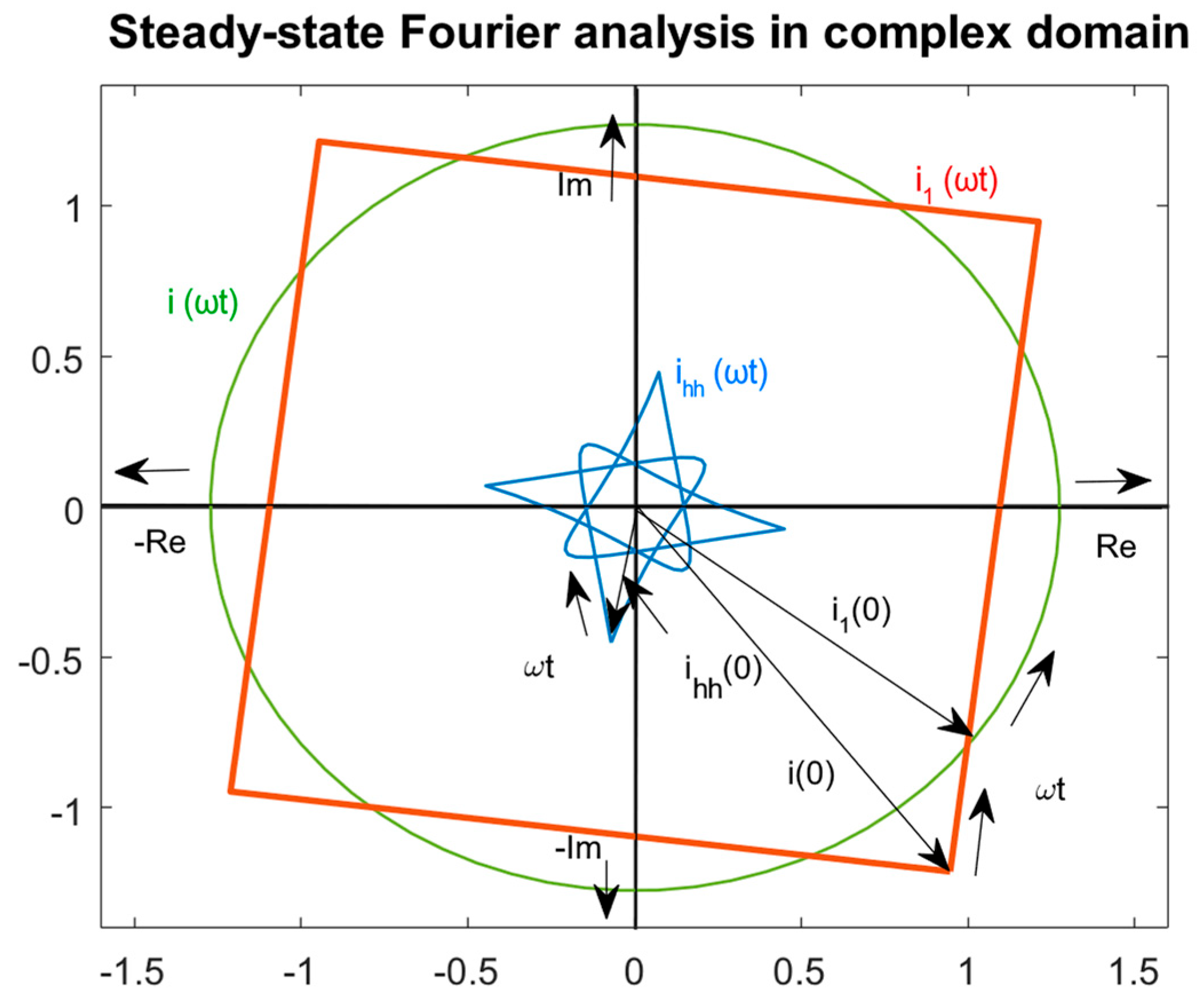
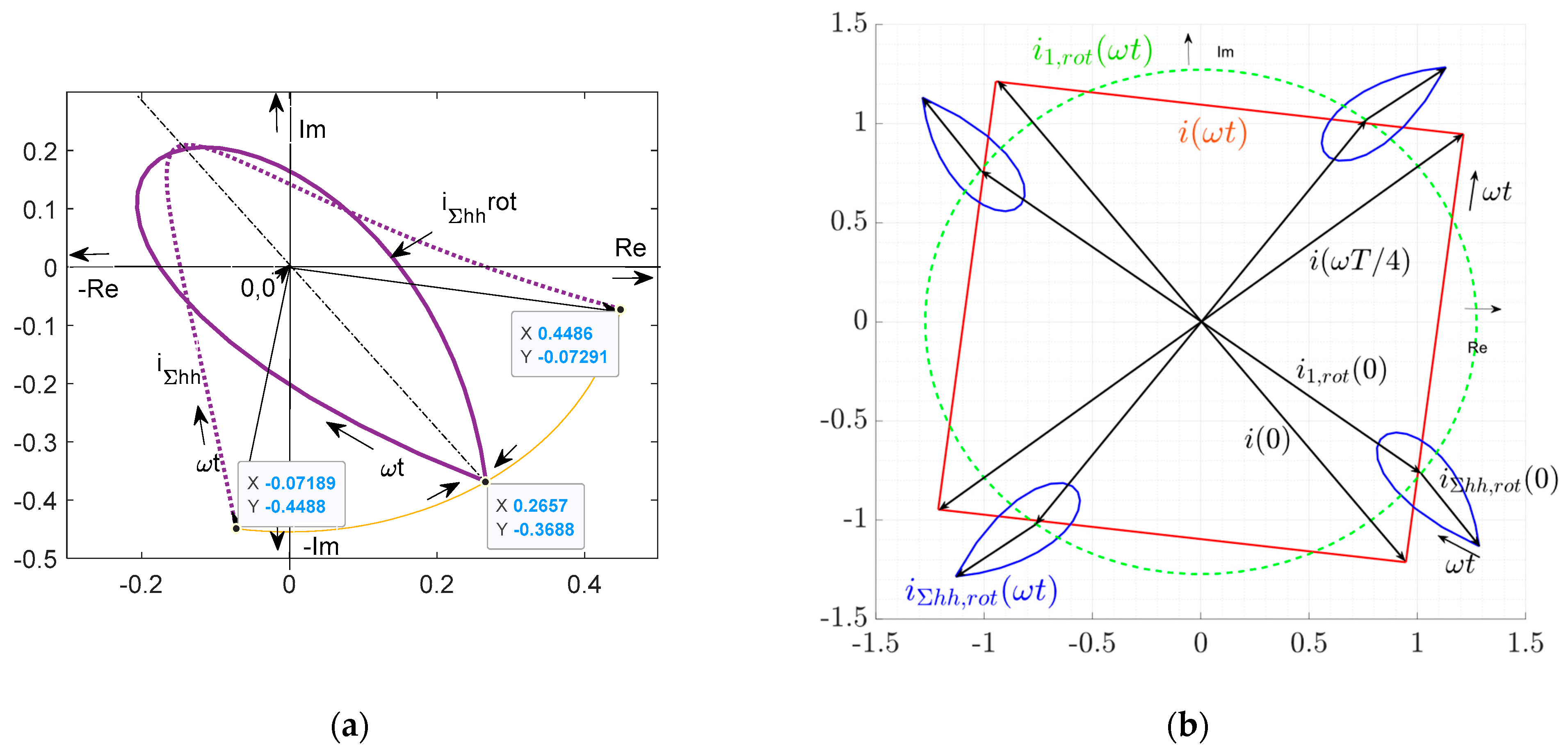
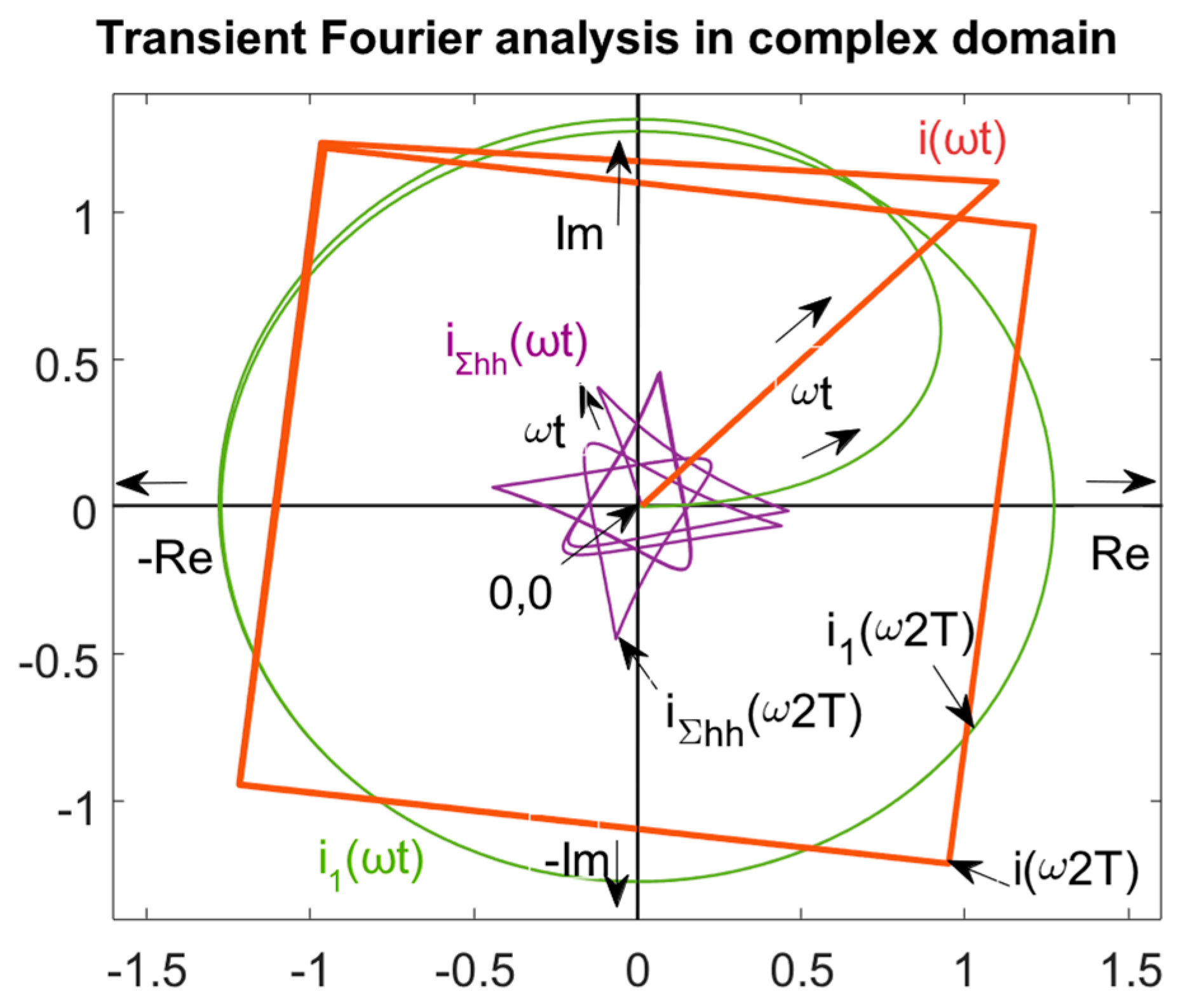
Analytical Solutions of Transient Values Using Fourier Series Using the Laplace–Carson Transform and Complex Time Vectors Inside One Period

Let us suppose a single electrical R-L circuit is supplied by harmonic voltage, as shown in Figure 2.

In the case of harmonic sinusoidal supply, it is valid.

$$u\left(t\right)=U_m\sin (\omega t+\delta ) \mathrm{o}\mathrm{r}$$

(5a)

$$u\left(t\right)=U_m\cos (\omega t+\delta ),$$

(5b)

where $\delta$ is a voltage connection angle to the load circuit or/and the initial angle of the time vector in the complex Gaussian plane. Adding a two-position switch in Figure 2b, where one of the positions closes the circuit, and the other grounds the R-L load, it is possible to reproduce the voltage profile on the R-L load of Figure 1a. Both curves in Figure 1 can be represented by the Fourier series.

Going back to the Fourier series, then using the relation Equations $\left(5\mathrm{a}\right)$ and $\left(5\mathrm{b}\right)$ we can write a projection in the complex domain

$$\mathit{U}\left(t\right)=\sum _{\nu =1}^{\mathrm{\infty }}{U}_{m,\nu }{\mathrm{e}}^{j\left({\omega }_{\nu }t+{\delta }_{\nu }\right)},$$

(6a)

where the angle frequency $\omega$ will be replaced by the frequency of the $\nu$-th harmonic ${\omega }_{\nu }$, the phase displacement $\phi$ by ${\phi }_{\nu }$, and $\delta$ by ${\delta }_{\nu }$.

After decomposing as a sum of the first and higher harmonic components, where the first term is a simple vector (${\mathit{U}}_1\left(t\right)$) starting at $\omega t=0$ rotated by an angle $\delta$, and the second one is the sum of the higher harmonic phasors ${\mathit{U}}_{\mathrm{n}}\left(t\right)$, we obtain

$$\mathit{U}\left(t\right)={\mathit{U}}_1\left(t\right)+{\mathit{U}}_{\mathrm{n}}\left(t\right).$$

(6b)

It is simpler to sum these two current vectors (right side of Equation (6b)) in a coordinate system fixed to the system’s real axis i.e. to the fundamental voltage vector. In this rotary coordinate system, the fundamental current is stationary, and the path of the current harmonics is a closed loop.

The graphic interpretation of the voltage vectors in the Gauss plane is shown in Figure 3.

Going back to the transfer analysis, each harmonic component of the sum in Equation (6a) can be further processed using Laplace or Laplace–Carson transform. So, by transforming any harmonic given by Equation (6a) we obtain

$$\mathit{U}\left(p\right)=\mathit{U}\left(0\right){\displaystyle \frac{1}{p-j\omega }}.$$

(7a)

using Laplace transform or

$$\mathit{U}\left(p\right)=\mathit{U}\left(0\right){\displaystyle \frac{p}{p-j\omega }}.$$

(7b)

using Laplace–Carson transform.

Comparing Equations $(7\mathrm{a},\mathrm{b})$ and $\left(4\right),$ we can see a considerable simplification of the notation.

Then, since the operator impedance $Z\left(p\right)=R+pL$, $I\left(0\right)=0$ and using Equation $\left(7\mathrm{b}\right),$ the complex time vector of the operator current gives

$$\mathit{I}\left(p\right)={\displaystyle \frac{\mathit{U}\left(0\right)}{L}}{\displaystyle \frac{p}{\left(p-j\omega \right)\left(p+\frac{R}{L}\right)}}.$$

(8)

where the roots of the denominator are

$$p_1=j\omega ;\hspace{1em}{p}_2=-{\displaystyle \frac{R}{L}}.$$

Applying inverse transform using Cauchy-Heaviside theorem

$$f\left(t\right)=\sum _{k=1}^N\underset{p\to p_k}{\lim }\left(p-p_k\right)\left[{\displaystyle \frac{F\left(p\right)}{p}}{e}^{p_{k}t}\right].$$

(9)

Then, the relationship is obtained

$$\mathit{I}\left(t\right)={\displaystyle \frac{\mathit{U}\left(0\right)}{L}}{\displaystyle \frac{1}{j\omega +\frac{R}{L}}}\left({\mathrm{e}}^{j\left(\omega t\right)}-{\mathrm{e}}^{-{\displaystyle \frac{R}{L}}t}\right).$$

(10a)

By introducing complex impedance $\mathit{Z}=\left|Z\right|{\mathrm{e}}^{j\phi }$ we obtain

$$\mathit{I}\left(t\right)={\displaystyle \frac{\mathit{U}\left(0\right)}{\mathit{Z}}}\left({\mathrm{e}}^{j\left(\omega t\right)}-{\mathrm{e}}^{-{\displaystyle \frac{R}{L}}t}\right).$$

(10b)

and consequently, respecting the different switch-on $\delta$ angle

$$\mathit{I}\left(t\right)={\displaystyle \frac{U_m}{\left|Z\right|}}\left({\mathrm{e}}^{j\left(\omega t+\delta -\phi \right)}-{\mathrm{e}}^{j\left(\delta -\phi \right)}{\mathrm{e}}^{-{\displaystyle \frac{R}{L}}t}\right).$$

(10c)

From this, Equation (10c) holds for the real part

$$i\left(t\right)={\displaystyle \frac{U_m}{\left|Z\right|}}\left[\mathrm{c}\mathrm{o}\mathrm{s}\left(\omega t+\delta -\phi \right)-\mathrm{c}\mathrm{o}\mathrm{s}\left(\delta -\phi \right){\mathrm{e}}^{-{\displaystyle \frac{R}{L}}t}\right],$$

(11a)

for $u\left(t\right)=U_m\cos (\omega t+\delta )$ or/and

$$i\left(t\right)={\displaystyle \frac{U_m}{\left|Z\right|}}\left[\mathrm{s}\mathrm{i}\mathrm{n}\left(\omega t+\delta -\phi \right)-\mathrm{s}\mathrm{i}\mathrm{n}\left(\delta -\phi \right){\mathrm{e}}^{-{\displaystyle \frac{R}{L}}t}\right],$$

(11b)

for $u\left(t\right)=U_m\sin (\omega t+\delta )$, respectively.

Supposing $t\to \mathrm{\infty },$ we can easily obtain the steady-state for variable $i\left(t\right)$, such as

$$i\left(t\right)={\displaystyle \frac{U_m}{\left|Z\right|}}\left[\mathrm{c}\mathrm{o}\mathrm{s}\left(\omega t+\delta -\phi \right)\right],$$

(11c)

for $u\left(t\right)=U_m\cos (\omega t+\delta )$.

The steady-state component is also—more easily—obtained using symbolic calculus and complex time vectors, respectively, directly without $\mathcal{L}\mathcal{}C$ transformation.

$$\mathit{I}\left(t\right)={\displaystyle \frac{U_m{\mathrm{e}}^{j(\omega t+\delta )}}{R+j\omega L}}={\displaystyle \frac{\mathit{U}\left(0\right){\mathrm{e}}^{j\left(\omega t\right)}}{\left|Z\right|{\mathrm{e}}^{j\phi }}}={\displaystyle \frac{\mathit{U}\left(0\right){\mathrm{e}}^{j\left(\omega t-\phi \right)}}{\left|Z\right|}},$$

(12a)

From where the real part is founded, the time waveform of the fundamental current variable $i\left(t\right)$,

$$i\left(t\right)={\displaystyle \frac{U_m}{\left|Z\right|}}\cos \left(\omega t+\delta -\phi \right).$$

(12b)

The time waveforms of the higher harmonics are similar, while the angle frequency $\omega$ will be replaced by the frequency of the $\nu$-th harmonic ${\omega }_{\nu }$, the phase displacement $\phi$ by ${\phi }_{\nu }$, and $\delta$ by ${\delta }_{\nu }$,

$$i_{\nu }\left(t\right)={\displaystyle \frac{{U_m}_{\nu }}{\left|Z_{\nu }\right|}}\cos \left({\omega }_{\nu },t+{\delta }_{\nu }-{\phi }_{\nu }\right).$$

(12c)

Respecting Equations (12b) and (12c), we can graphically image in the complex Gauss plane in Figure 4.

The course of higher harmonics in the range $0-\pi /2$ is shown separately in Figure 5a in both stationary and revolving coordinate systems [7] and for the transformation of the vector of higher harmonics, the relation applies

$${\mathit{i}}_{hh,rot}\left(t\right)={\mathit{i}}_{hh}\left(t\right)\mathrm{e}\mathrm{x}\mathrm{p}\left[-j\left(\omega t-\pi /2\right)\right].$$

(13)

Adding the vectors of fundamental and higher harmonic components—similarly as in the time domain—we obtain

$$\mathit{I}\left(t\right)={\mathit{I}}_1\left(t\right)+U_{m,\nu }\sum _{\nu =3}^{\mathrm{\infty }}{\displaystyle \frac{1}{\left|Z_{\nu }\right|}}{\mathrm{e}}^{j\left({\omega }_{\nu }t-{\phi }_{\nu }\right)}.$$

(13a)

Since the first term is a simple rotating vector (i.e., phasor) starting at $\omega t=0$ rotated by an angle $-\phi$, the second one is the sum of the higher harmonic phasors ${\mathit{I}}_{\nu }\left(t\right)$.

The obtained result can be displayed, as in Figure 5a,b.

The fundamental harmonic in the time domain is given by Equation (14a) if the switching angle δ is zero.

$$i\left(t\right)={\displaystyle \frac{U_m}{\left|Z\right|}}\left[\mathrm{c}\mathrm{o}\mathrm{s}\left(\omega t+\delta -\phi \right)\right],$$

(14a)

for $u\left(t\right)=U_m\cos (\omega t+\delta )$.

The transient component one obtains from Equation $\left(11\mathrm{a}\right)$ for ‘cosine’ supply (with cosine components)

$$i\left(t\right)={\displaystyle \frac{U_m}{\left|Z\right|}}\left[-\mathrm{c}\mathrm{o}\mathrm{s}\left(\delta -\phi \right){\mathrm{e}}^{-{\displaystyle \frac{R}{L}}t}\right].$$

(14b)

Or Equation $\left(11\mathrm{b}\right)$ for ‘sine’ supply (with sine components).

Supposing $\delta$ equals 0, the steady state is simply

$${\mathit{I}}_{\nu }\left(t\right)={\displaystyle \frac{{U_m}_{\nu }}{\left|Z_{\nu }\right|}}{\mathrm{e}}^{j\left({\omega }_{\nu }t-{\phi }_{\nu }\right)},$$

(14c)

where $U_{m,\nu }=U_m/\nu$ and thus the amplitude spectrum is monotonically decreasing.

Using the above approach given by Equations (7a,b)–(11c), it is possible to calculate the current time course of any $\mathrm{n}$-th harmonic, thus

$${\mathit{I}}_{\nu }\left(t\right)={\displaystyle \frac{{U_m}_{\nu }}{\left|Z_{\nu }\right|}}\left({\mathrm{e}}^{j\left({\omega }_{\nu }t+{\delta }_{\nu }-{\phi }_{\nu }\right)}-{\mathrm{e}}^{j\left({\delta }_{\nu }-{\phi }_{\nu }\right)}{\mathrm{e}}^{-{\displaystyle \frac{R}{L}}t}\right).$$

(15a)

and its real part

$$i_{\nu }\left(t\right)={\displaystyle \frac{{U_m}_{\nu }}{\left|Z_{\nu }\right|}}\left[\mathrm{c}\mathrm{o}\mathrm{s}\left({\omega }_{\nu }t+{\delta }_{\nu }-{\phi }_{\nu }\right)-\mathrm{c}\mathrm{o}\mathrm{s}\left({\delta }_{\nu }-{\phi }_{\nu }\right){\mathrm{e}}^{-{\displaystyle \frac{R}{L}}t}\right].$$

(15b)

So, the total transient course will be

$$i_{tot}\left(t\right)={\displaystyle \frac{4}{\pi }}{U}_m\sum _{\nu =1}^{\mathrm{\infty }}{\displaystyle \frac{1}{\nu \left|Z_{\nu }\right|}}\left[\mathrm{c}\mathrm{o}\mathrm{s}\left({\omega }_{\nu }t+{\delta }_{\nu }-{\phi }_{\nu }\right)-\mathrm{c}\mathrm{o}\mathrm{s}\left({\delta }_{\nu }-{\phi }_{\nu }\right){\mathrm{e}}^{-{\displaystyle \frac{R}{L}}t}\right].$$

(16)

Respecting Equations (15a) and (16), we can graphically image the complex Gauss plane in Figure 6.

3. Transient Analysis of PES System Using Fourier Integral Transform

Since the Fourier transform [10] is defined over the entire time domain, not just for positive time values, it poses a challenge in circuit analysis where, as mentioned earlier, the forcing functions and their responses typically begin at $t=0$. For such functions, the Fourier transform can be expressed as

$$\mathit{F}\left(j\omega \right)=\underset{-\mathrm{\infty }}{\overset{\mathrm{\infty }}{\int }}u\left(t\right)f\left(t\right)e^{-j\omega t}\mathrm{d}t=\underset{0}{\overset{\mathrm{\infty }}{\int }}f\left(t\right)e^{-j\omega t}\mathrm{d}t$$

(17)

where $u\left(t\right)$ means the unit-step function at $t=0$.

In comparison to the Laplace transform, for a function that meets the necessary conditions, the Fourier transform can be obtained simply by replacing s with $j\omega$ in the Laplace transform, i.e.,

$$\mathit{F}\left(j\omega \right)=\mathit{F}{(\left.s)\right|}_{\mathit{s}=j\omega }$$

(17a)

This approach for determining the spectral components of most non-periodic functions is both the simplest and most convenient method.

In the following power electronics applications, we address the transient analysis using two methods: first, by employing Fourier series/expansions with an emphasis on steady-state operation, and then by using the Fourier transform with a focus on transient analysis.

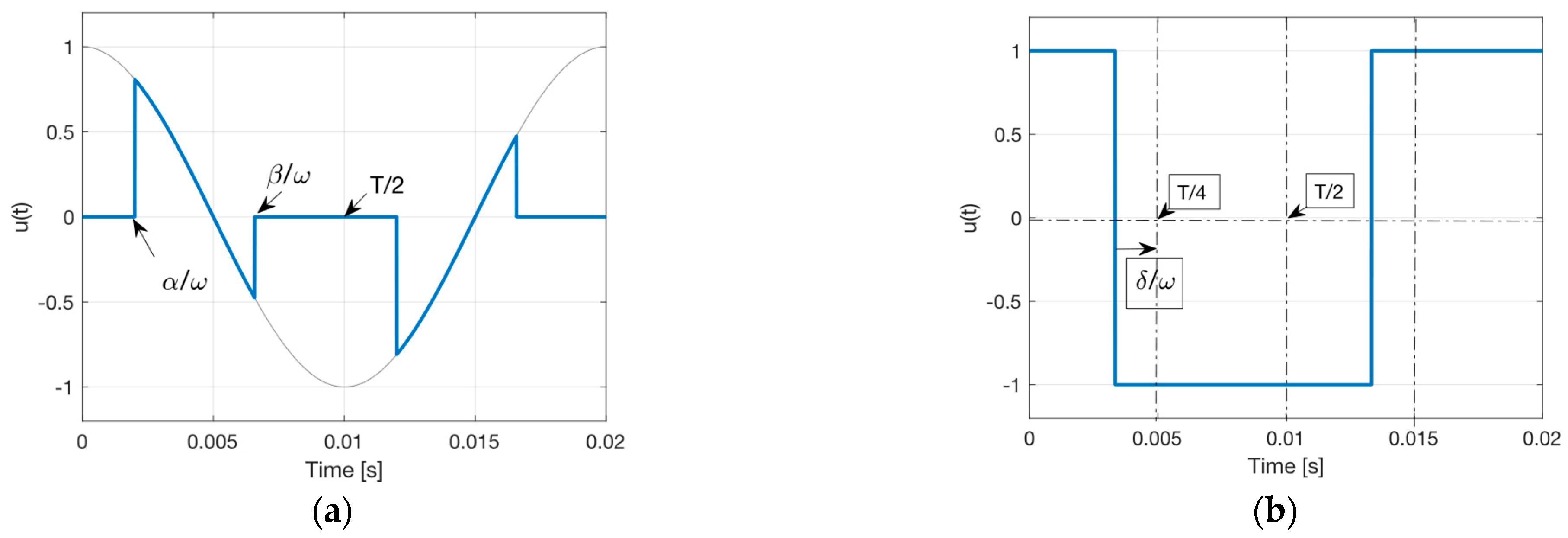
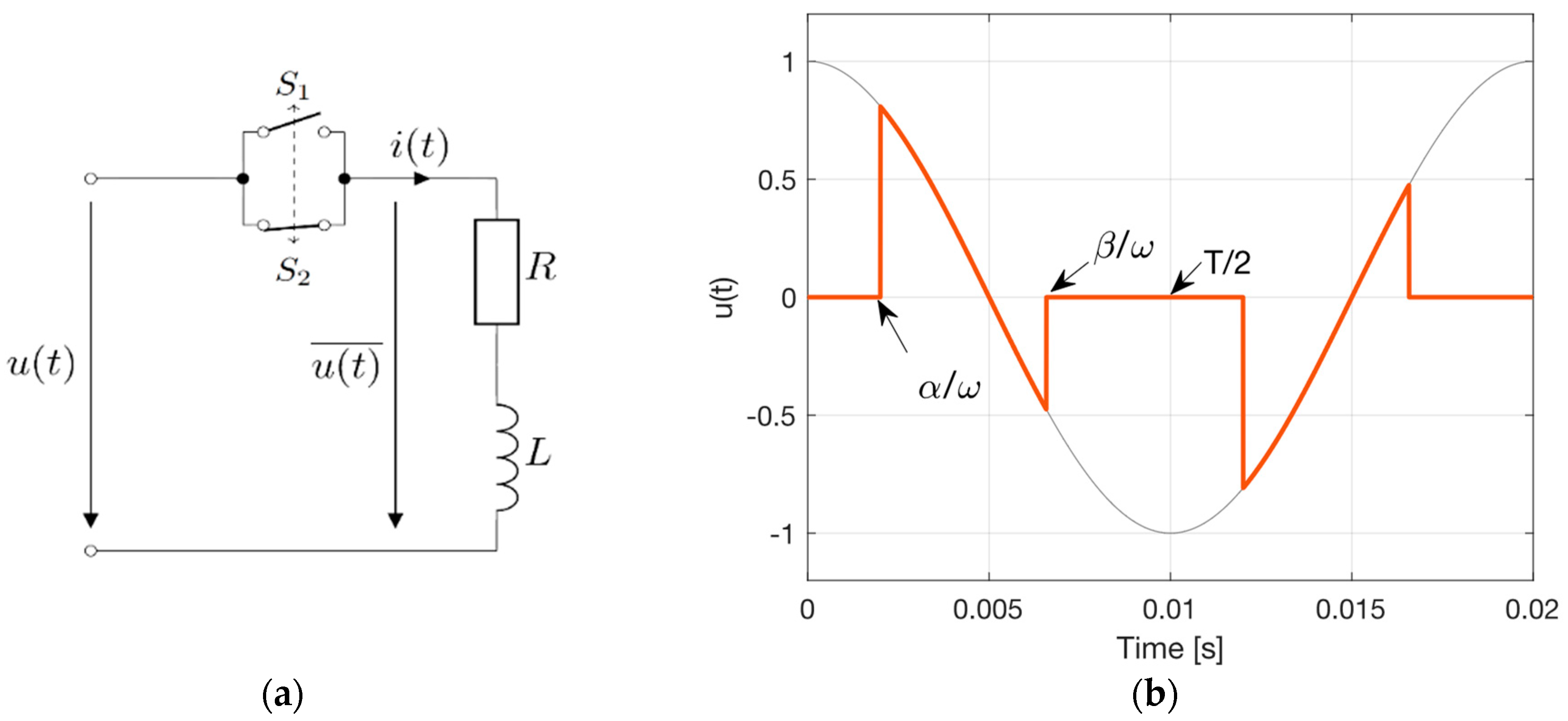
3.1. Case of Passive Resistive-Inductive Load Without Back-Electromotive Force (emf)

The connection of the electrical circuit is shown in Figure 7a, and the principal courses of the input and output (load) voltages in Figure 7b.

For AC symmetric waveform is valid

$$f\left(t\right)=a_1\cos \omega t+\cdots +a_{\nu }\cos \nu \omega t+b_1\sin \omega t+\cdots +b_{\nu }\sin \nu \omega t.$$

(18)

Fourier coefficients for the ν-harmonics type of cosine (see Appendix A)

$$\begin{gathered} a_{\nu }=U_m{\displaystyle \frac{2}{T}}\underset{0}{\overset{T}{\int }}\cos \omega t.\cos \nu \omega t \mathrm{d}t \\ {=U}_m{\displaystyle \frac{1}{\pi }}\left[{\displaystyle \frac{\mathrm{s}\mathrm{i}\mathrm{n}\left(1-\nu \right)\beta -\mathrm{s}\mathrm{i}\mathrm{n}\left(1-\nu \right)\alpha }{\left(1-\nu \right)}}+{\displaystyle \frac{\sin \left(1+\nu \right)\beta -\sin \left(1+\nu \right)\alpha }{\left(1+\nu \right)}}\right]. \end{gathered}$$

(18a)

As $=2k+1,$ then $1-v=2k$ and $1+v=2k+2$

$$a_{\nu }=U_m{\displaystyle \frac{1}{\pi }}\left[{\displaystyle \frac{\mathrm{s}\mathrm{i}\mathrm{n}2k\beta -\mathrm{s}\mathrm{i}\mathrm{n}2k\alpha }{2k}}+{\displaystyle \frac{\sin 2\left(k+1\right)\beta -\sin 2\left(k+1\right)\alpha }{2\left(k+1\right)}}\right].$$

(18b)

And since

$$\underset{k=0}{\lim }{\displaystyle \frac{\mathrm{s}\mathrm{i}\mathrm{n}2k\beta -\mathrm{s}\mathrm{i}\mathrm{n}2k\alpha }{2k}}=\beta -\alpha .$$

Then

$$a_1=U_m{\displaystyle \frac{1}{\pi }}\left[\left(\beta -\alpha \right)-{\displaystyle \frac{\sin 2\beta -\sin 2\alpha }{2}}\right].$$

(18c)

Similarly for sine coefficients (see Appendix B)

$$\begin{gathered} b_{\nu }=U_m{\displaystyle \frac{2}{T}}\underset{0}{\overset{T}{\int }}\cos \omega t.\sin \nu \omega t \mathrm{d}t \\ {=U}_m{\displaystyle \frac{1}{\pi }}{\left(-1\right)}^{\nu }\left[{\displaystyle \frac{\cos \left(\mathrm{n}+1\right)\beta -\cos \left(\mathrm{n}-1\right)\alpha }{\nu -1}}-{\displaystyle \frac{\cos \left(\mathrm{n}+1\right)\beta -\cos \left(\mathrm{n}+1\right)\alpha }{\nu +1}}\right]. \end{gathered}$$

(19a)

As $=2k+1,$ then $1-\nu =2k$ and $1+\nu =2k+2$

$$b_{\nu }=U_m{\displaystyle \frac{1}{\pi }}\left[{\displaystyle \frac{\mathrm{c}\mathrm{o}\mathrm{s}2k\beta -\mathrm{c}\mathrm{o}\mathrm{s}2k\alpha }{2k}}+{\displaystyle \frac{\cos 2\left(k+1\right)\beta -\cos 2\left(k+1\right)\alpha }{2\left(k+1\right)}}\right].$$

(19b)

And since

$$\underset{k=0}{\lim }{\displaystyle \frac{\mathrm{s}\mathrm{i}\mathrm{n}2k\beta -\mathrm{s}\mathrm{i}\mathrm{n}2k\alpha }{2k}}=0,$$

$$b_1={-U}_m{\displaystyle \frac{1}{\pi }}{\displaystyle \frac{\cos 2\beta -\cos 2\alpha }{2}}.$$

(19c)

Thus, the input voltage expressed by the Fourier series is defined using Equation $\left(1\right)$.

Then, for the load current using Equations (18b) and (19)

$$i\left(t\right)=U_m\sum _{\nu =1}^{\mathrm{\infty }}{c}_{\nu }{\displaystyle \frac{\cos \left(\nu \omega t-{\vartheta }_{\nu }-{\phi }_{\nu }\right)-\cos \left({\vartheta }_{\nu }-{\phi }_{\nu }\right)e^{-t/{\tau }_{\nu }}}{\sqrt{R^2+{\left(\nu \omega L\right)}^2}}}$$

(20a)

where ${\phi }_{\nu }=\mathrm{a}\mathrm{t}\mathrm{a}\mathrm{n}\left(\mathrm{n}\omega L/R\right)$ and ${\tau }_{\nu }\equiv {\tau }_1=L/R$.

Note: with a purely inductive load ($R=0$), the transient component $e^{-t/{\tau }_{\nu }}$ will be zero

$$i\left(t\right)=U_m\sum _{\nu =1}^{\mathrm{\infty }}{c}_{\nu }{\displaystyle \frac{\cos \left(\nu \omega t-{\vartheta }_{\nu }-{\phi }_{\nu }\right)}{\sqrt{R^2+{\left(\nu \omega L\right)}^2}}}.$$

(20b)

Note: if $\alpha =0$ and $R=0,$ the load current will be a purely sinusoidal one, i.e., for the fundamental harmonic

$$i\left(t\right)={\displaystyle \frac{U_m}{\left|Z\right|}}\cos \left(\omega t-\phi \right).$$

If the load current $i\left(t\right)$ will be zero, then $\omega t=\beta$ and so

$$\sum _{\nu =1}^{\mathrm{\infty }}{c}_{\nu }{\displaystyle \frac{\cos \left(\nu \beta -{\vartheta }_{\nu }-{\phi }_{\nu }\right)}{\sqrt{R^2+{\left(\nu \omega L\right)}^2}}}=0$$

(20c)

from where it is possible to obtain the angle $\beta$, e.g., in an iterative way. If $\beta =\pi -\alpha ,$ it means that the load is purely inductive.

The graphic interpretation of Equation $\left(20\mathrm{b}\right)$ is shown in Figure 8. The parameters of the system are given in

Table 1. Parameters of the system.

Um [V]	${\mathit{f}}_1$ [Hz]	R [W]	L [mH]	Z [W]	${\mathit{\tau }}_1$ [ms]	${\mathit{\phi }}_1$ [deg]
325	50	18.4	43.93	23	2.3875	36.76

.

The solution to the transient phenomenon of the system is significant only when the current is continuous, with the turn-on angle equal to the phase shift angle, i.e., 36.76 − 90 = −53.24 electrical degrees. Under this condition, the current will be purely sinusoidal. During the transient state, when switching occurs at α = 0, the current will increase from zero to its steady-state value according to the modified form of relation Equation (11a) for the fundamental harmonic

$$i_{RL}\left(t\right)={\displaystyle \frac{U_m}{Z}}{\left.\left[\mathrm{c}\mathrm{o}\mathrm{s}\left({\omega }_{1}t+\mathrm{a}-{\phi }_1\right)-{\mathrm{c}\mathrm{o}\mathrm{s}\left(\mathrm{a}-{\phi }_1\right)e}^{-t/{\tau }_1}\right]\right|}_{\alpha =0}.$$

(21)

The waveform for $\alpha =0$ is shown in Figure 9.

Since the equation consists of steady- and transient-state components, we can write

$$\begin{gathered} {\mathit{F}}_{i_{RL}}\left(j\omega \right)={\mathit{F}}_{st-st}\left(j\omega \right)+{\mathit{F}}_{trans}\left(j\omega \right) \\ ={\displaystyle \frac{U_m}{Z}}\underset{0}{\overset{\mathrm{\infty }}{\int }}\mathrm{c}\mathrm{o}\mathrm{s}\left({\omega }_{1}t-{\phi }_1\right)e^{-j\omega t}\mathrm{d}t+{\displaystyle \frac{U_m}{Z}}\underset{0}{\overset{\mathrm{\infty }}{\int }}\mathrm{c}\mathrm{o}\mathrm{s}\left(-{\phi }_1\right)e^{-t/{\tau }_1}{e}^{-j\omega t}\mathrm{d}t. \end{gathered}$$

(22)

The Fourier transform of $i_{RL}\left(t\right)$ function Equation (21) can be derived (a simplified approach [1,11]) with the time-shift rule,

$$f\left(t\pm t_1\right)\leftrightarrow e^{j\omega t_1}\mathcal{F}\left\{f\left(t\right)\right\},$$

(23)

where $t_1={\displaystyle \frac{{\phi }_1}{{\omega }_1}}$.

Then, for steady-state component

$$\begin{gathered} {\mathit{F}}_{st-st}\left(j\omega \right)=e^{j{\phi }_1}{\mathcal{F}}_{st-st}\left\{u\left(t\right)\mathrm{c}\mathrm{o}\mathrm{s}{\omega }_{1}t\right\}={\displaystyle \frac{U_m}{Z}}{e}^{j{\phi }_1}{\mathcal{F}}_{st-st}\left\{{\displaystyle \frac{1}{2}}\left[e^{j{\omega }_{1}t}+e^{-j{\omega }_{1}t}\right]\right\} \\ ={\displaystyle \frac{U_m}{Z}}{\displaystyle \frac{1}{2}}{e}^{j{\phi }_1}\left\{{\mathit{F}}_u\left[j\left(\omega -{\omega }_1\right)\right]+{\mathit{F}}_u\left[j\left(\omega +{\omega }_1\right)\right]\right\} \\ ={\displaystyle \frac{U_m}{Z}}{\displaystyle \frac{1}{2}}{e}^{j\omega {\displaystyle \frac{{\phi }_1}{{\omega }_1}}}\left[\pi \delta \left(\omega -{\omega }_1\right)+{\displaystyle \frac{1}{j\left(\omega -{\omega }_1\right)}}+\pi \delta \left(\omega +{\omega }_1\right)+{\displaystyle \frac{1}{j\left(\omega +{\omega }_1\right)}}\right] \\ ={\displaystyle \frac{U_m}{Z}}\left\{{\displaystyle \frac{\pi }{2}}\left[\delta \left(\omega -{\omega }_1\right)+\delta \left(\omega +{\omega }_1\right)\right]e^{j{\phi }_1}+{\displaystyle \frac{j\omega }{\left({{\omega }_1}^2{-\omega }^2\right)}}{e}^{j{\phi }_1}\right\}. \end{gathered}$$

(24)

And, for transient component

$${\mathit{F}}_{trans}\left(j\omega \right)={\mathcal{F}}_{trans}\left\{{\displaystyle \frac{U_m}{Z}}\mathrm{c}\mathrm{o}\mathrm{s}\left(-{\phi }_1\right)e^{-t/{\tau }_1}\right\}={\displaystyle \frac{U_m}{Z}}\cos {\phi }_1{\displaystyle \frac{1}{j\omega +\frac{1}{{\tau }_1}}}.$$

(25)

The graphic interpretation of the amplitude spectra of both components is shown in Figure 10 in the relative p.u. units (i.e., $U_m/Z\equiv 1)$.

Given that the time constant ${\tau }_1$ is relatively small (2.3875 ms), which is less than one-fourth of the time period, the predominant component of the response is the steady-state component.

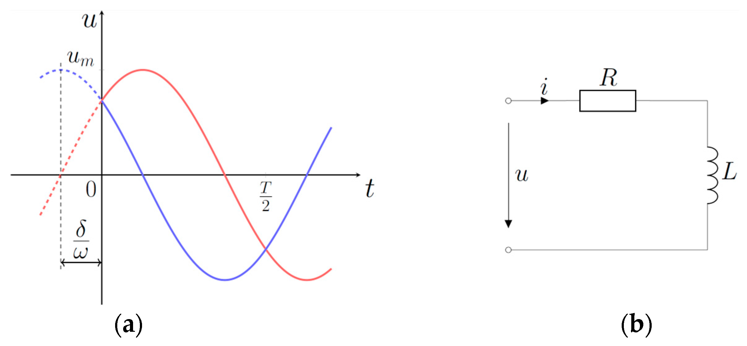
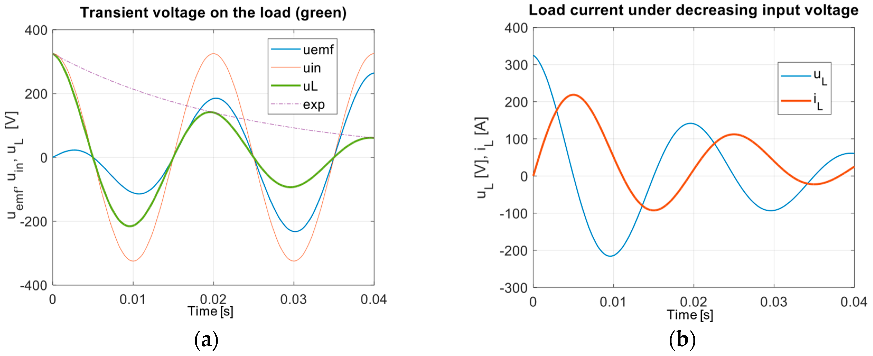
3.2. Case of Active-Inductive Load with Back-Emf

The connection of the electrical circuit is shown in Figure 11, and the principal time waveforms of the input and output (load) voltages in Figure 7b, where the input voltage $u_{in}\left(t\right)$ is harmonic cosine function, and S1 and S2 are electronic switches.

The Fourier coefficients of that series are calculated by Euler relations.

If $\beta =\pi -\alpha$ using Appendix C

$$\begin{gathered} a_1={\displaystyle \frac{8}{T}}\underset{{\displaystyle \frac{\alpha }{\omega }}}{\overset{{\displaystyle \frac{T}{4}}}{\int }}\cos \omega t.\cos \omega t \mathrm{d}t={\displaystyle \frac{2}{\pi }}\underset{\alpha }{\overset{\pi }{\int }}{\cos }^2\omega t \mathrm{d}\mathsf{\omega }t \\ =1-{\displaystyle \frac{2\alpha }{\pi }}-{\displaystyle \frac{\sin 2\alpha }{\pi }}. \end{gathered}$$

(26a)

or

$$\begin{gathered} ={\displaystyle \frac{2}{\pi }}\underset{\alpha }{\overset{\pi /2}{\int }}\left(1+\mathrm{c}\mathrm{o}\mathrm{s}2\omega t\right) \mathrm{d}\mathsf{\omega }t={\displaystyle \frac{2}{\pi }}{\left[\omega t\right]}_{\alpha }^{\pi /2}+{\displaystyle \frac{1}{\pi }}{\left[\sin 2\omega t\right]}_{\alpha }^{\pi /2} \\ ={\displaystyle \frac{2}{\pi }}\left({\displaystyle \frac{\pi }{2}}-\alpha \right)+{\displaystyle \frac{1}{\pi }}\left(\sin \pi -\sin 2\alpha \right)=1-{\displaystyle \frac{2\alpha }{\pi }}-{\displaystyle \frac{\sin 2\alpha }{\pi }}. \end{gathered}$$

(26b)

The same result we obtain using Equation $\left(18\mathrm{c}\right)$ for $\beta =\pi -\alpha$

$$a_1=U_m{\displaystyle \frac{1}{\pi }}\left[\left(\pi -\alpha -\alpha \right)-{\displaystyle \frac{\sin 2\left(\pi -\alpha \right)-\sin 2\alpha }{2}}\right]=U_m\left(1-{\displaystyle \frac{2\alpha }{\pi }}-{\displaystyle \frac{\mathrm{s}\mathrm{i}\mathrm{n}2\alpha }{2\pi }}\right).$$

(26c)

Similarly, for the sine coefficient of fundamental harmonic

$$\begin{gathered} b_1={\displaystyle \frac{2}{\pi }}\underset{\alpha }{\overset{\pi }{\int }}\cos \omega t.\sin \omega t \mathrm{d}\mathsf{\omega }t={\displaystyle \frac{1}{\pi }}\underset{\alpha }{\overset{\pi }{\int }}\sin 2\omega t \mathrm{d}\mathsf{\omega }t \\ ={\displaystyle \frac{1}{\pi }}\underset{\alpha }{\overset{\pi }{\int }}\sin 2\omega t \mathrm{d}\mathsf{\omega }t={\displaystyle \frac{1}{\pi }}(\underset{\alpha }{\overset{{\displaystyle \frac{\pi }{2}}}{\int }}+\underset{{\displaystyle \frac{\pi }{2}}}{\overset{\pi -\alpha }{\int }})\sin 2\omega t \mathrm{d}\mathsf{\omega }t \\ ={\displaystyle \frac{1}{2\pi }}\left[\cos 2\alpha -\left(-1\right)+\left(-1\right)-\cos 2\alpha \right]=0. \end{gathered}$$

(26d)

Checking, $\alpha =0,A1=1$

$$u\left(t,\alpha \right)=U_m\sum _{\nu =1}^{\mathrm{\infty }}{\left(-1\right)}^{{\displaystyle \frac{\nu -1}{2}}}{\displaystyle \frac{A_{\nu }}{\nu }}\cos \nu \omega t.$$

(27)

Fundamental harmonic max value

$$I_{1m}={\displaystyle \frac{2}{\pi }}\underset{\alpha }{\overset{\pi -\alpha }{\int }}{\displaystyle \frac{U_m}{\omega L}}\left(\mathrm{c}\mathrm{o}\mathrm{s}\omega t+\mathrm{c}\mathrm{o}\mathrm{s}\alpha \right)\mathrm{c}\mathrm{o}\mathrm{s}\omega t.\mathrm{d}\omega t={\displaystyle \frac{V_m}{\omega L}}{\displaystyle \frac{2}{\pi }}\left({\displaystyle \frac{1}{2}}\mathrm{s}\mathrm{i}\mathrm{n}2\alpha +\pi -\alpha \right).$$

(27a)

The parameters of the system are given in

Table 2. Parameters of the system $\alpha =36°,\mathrm{i}.\mathrm{e}.,\pi /5$.

Um [V]	${\mathit{f}}_1$ [Hz]	R [W]	L [mH]	Z [W]	${\mathit{\tau }}_{\mathit{r}\mathit{i}\mathit{s}\mathit{e}}$ [ms]	${\mathit{\phi }}_1$ [deg]
325	50	18.4	43.93	23	10 τ1	90

.

The graphic interpretation of Equation $\left(20\right)$ is shown in Figure 12a,b.

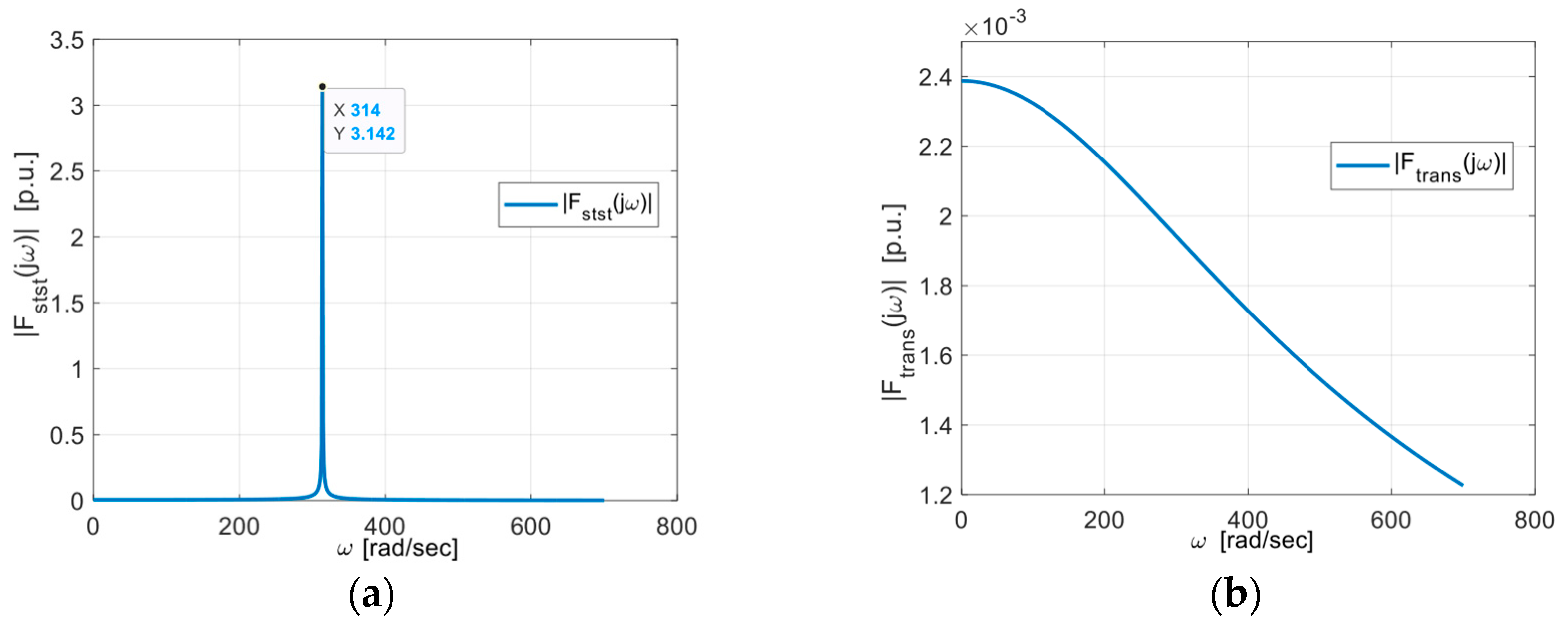
3.3. Transient Analysis Using Fourier Transform (and Under Decreasing Cosine Function)

Assuming an exponentially increasing back-emf voltage, such as during the start-up of an electric motor, and a constant harmonic input voltage, the voltage across the load (inductor) will follow a decreasing cosine function

$$u_L\left(t\right)=U_m\mathrm{c}\mathrm{o}\mathrm{s}{\omega }_{1}t.{\mathrm{e}}^{-{\displaystyle \frac{t}{{\tau }_{rise}}}},$$

(28)

where ${\tau }_{rise}$ respects a rise in the back-emf voltage, as shown in Figure 13a (green). If we take $u_L\left(t\right)$ according to (28), the corresponding load current of the inductor can be calculated, as shown in Figure 13b (red).

Applying the Fourier transform on the transient voltage $u_L\left(t\right),$ we can write [1]

$${\mathit{F}}_u\left(j\omega \right)=U_m\underset{0}{\overset{\mathrm{\infty }}{\int }}{e}^{-at}\mathrm{c}\mathrm{o}\mathrm{s}{\omega }_{1}t{e}^{-j\omega t}\mathrm{d}t,$$

(29)

where $a(=1/{\tau }_{rise})$ represents a damping of the circuit and ${\omega }_1$ is an angular frequency of the input voltage.

The infinitive integral $\int \left(.\right)$ can be calculated by substitution or per partes methods with the result

$$\int \left(.\right)={\displaystyle \frac{e^{-(a+j\omega )}}{{\left[-(a+j\omega )\right]}^2+{{\omega }_0}^2}}\left(-\left(a+j\omega \right)\mathrm{c}\mathrm{o}\mathrm{s}{\omega }_{1}t+{\omega }_0\mathrm{s}\mathrm{i}\mathrm{n}{\omega }_{1}t\right),$$

(30)

with use of the Euler formula as a substitution for $\mathrm{c}\mathrm{o}\mathrm{s}{\omega }_{1}t$.

So, after the establishment of integration boundaries

$$\underset{0}{\overset{\mathrm{\infty }}{\int }}\left(.\right)=\left[0-{\displaystyle \frac{-\left(a+j\omega \right)}{{\left[-(a+j\omega )\right]}^2+{{\omega }_1}^2}}\right]=\left[{\displaystyle \frac{\left(a+j\omega \right)}{{(a+j\omega )}^2+{{\omega }_1}^2}}\right],$$

(30a)

thus

$${\mathit{F}}_u\left(j\omega \right)=U_m{\displaystyle \frac{a+j\omega }{a+{{\omega }_1}^2-{\omega }^2+j2a\omega }}.$$

(31)

The magnitude spectrum of ${\mathit{F}}_u\left(j\omega \right)$

$$\left|{\mathit{F}}_u\left(j\omega \right)\right|=U_m\sqrt{{\displaystyle \frac{a^2+{\omega }^2}{{\left(a^2+{{\omega }_1}^2-{\omega }^2\right)}^2+4a^2{\omega }^2}}}$$

(31a)

The graphic interpretation of the magnitude spectra of $\left|{\mathit{F}}_u\left(j\omega \right)\right|$ is shown in Figure 14 in the relative p.u. units (i.e., $U_m\equiv 1)$.

The phase spectrum of $\mathit{F}\left(j\omega \right)$ we can calculate as an arctan function of the share quotient of the imaginary and real part of the magnitude spectrum ($\left|{\mathit{F}}_u\left(j\omega \right)\right|$)

$$\left(\omega \right)={\mathrm{t}\mathrm{a}\mathrm{n}}^{-1}{\displaystyle \frac{Im\left\{{\mathit{F}}_u\left(j\omega \right)\right\}}{Re\left\{{\mathit{F}}_u\left(j\omega \right)\right\}}}.$$

(32)

Similarly, as for $u_L\left(t\right)$—if we admit that the load current is decreasing the quasi sinusoidal function (Figure 15)—we can apply its Fourier transform

$${\mathit{F}}_i\left(j\omega \right)=I_m\underset{0}{\overset{\mathrm{\infty }}{\int }}{e}^{-at}\left[\mathrm{s}\mathrm{i}\mathrm{n}{(\omega }_{1}t-{\phi }_L)+\mathrm{s}\mathrm{i}\mathrm{n}{\phi }_L\right]e^{-j\omega t}\mathrm{d}t,$$

(33)

where the maximal value of the load current

$$I_m={\displaystyle \frac{U_m}{L\sqrt{a^2+{\omega }_1^2}}},$$

(34)

and ${\phi }_L={\mathrm{t}\mathrm{a}\mathrm{n}}^{-1}\left({\displaystyle \frac{a}{{\omega }_1}}\right)$ where $a=1/{\tau }_{rise}$ as mentioned above.

The magnitude spectrum of the current Fourier transform $\left|{\mathit{F}}_i\left(j\omega \right)\right|$ is depicted in Figure 15.

4. Discussion and Conclusions

From the results shown in Figure 10b and Figure 15, it is evident that during transient states, both the analyzed quantities exhibit a continuous spectrum of harmonic components, including the fundamental frequency. This implies that the electrical power, as a product of current and voltage, will contain distortion components, even in harmonic networks with linear loads (resistive, inductive, or both). Although this observation may seem unexpected, it is a significant contribution to practical applications.

While classical Fourier analysis, including its application to transient signal analysis, may not be as effective as other methods, it still offers distinct advantages:

• It provides insight into the harmonic content of the signal;
• It allows for the straightforward calculation of harmonic distortion [12].

The function being analyzed does not need to be analytically defined over the entire period and can be represented using methods like look-up tables.

When performing analysis in the complex domain, regardless of the method used, it enables the calculation of the effective values of quantities and the average power components. This is especially useful, as it allows for time savings in repeated calculations—1/4 of a time period for single-phase systems and 1/6 for three-phase systems. The Fourier transform also demonstrates that even with harmonic power supplies and linear time-invariant (LTI) loads, transient states generate a continuous spectrum of higher harmonics (Figure 10b, Figure 14 and Figure 15). In repeated or long-term START-STOP regimes, this could lead to excessive current stresses on system components, such as power transformers.

Additionally, when combined with the Laplace or Laplace–Carson transforms, Fourier analysis becomes a powerful tool for solving transient phenomena, especially when addressing steady-state conditions within a single time period.

This paper introduces two novel and effective approaches to transient analysis:

• The combined use of Fourier and L-C transforms in the complex domain, which significantly simplifies the computation of the original function (Figure 3, Figure 4, Figure 5 and Figure 6);
• The application of Fourier transforms for analyzing transient states in electrical systems, particularly in electrotechnical applications (Figure 10b, Figure 14 and Figure 15);
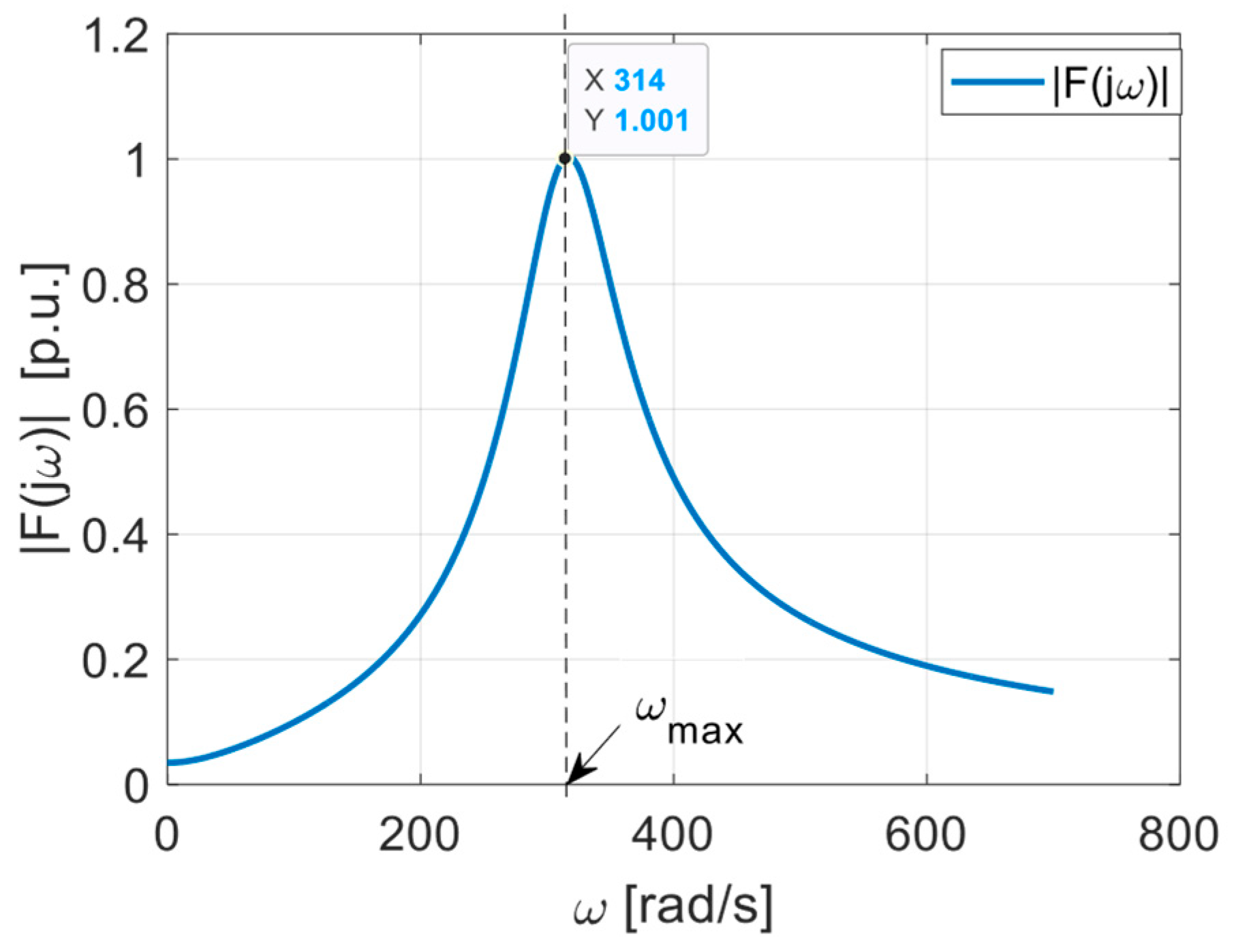
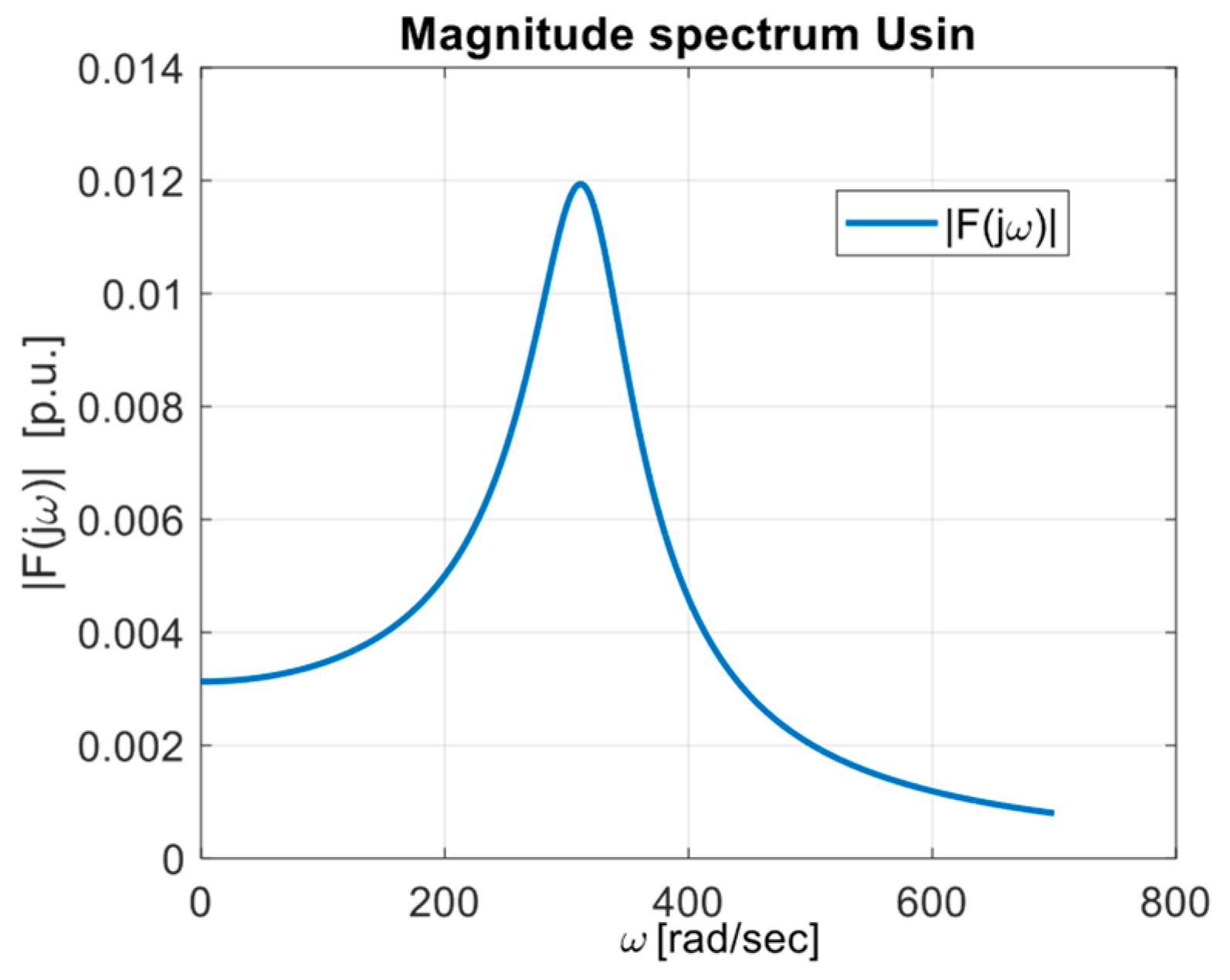
• The unique ability of this transformation to provide magnitude and phase frequency spectra, which are not easily obtained through other methods, demonstrates its utility [13].

In conclusion, this work presents a significant advancement in transient Fourier analysis, offering novel insights into the behavior of individual harmonics and their superposition in dynamic systems. The integration of complex time-domain analysis and the innovative techniques presented here hold considerable potential for further developments in this field.

References

1. Shenkman, A.L. Transient analysis using the Fourier transform. In Transient Analysis of Electric Power Circuits Handbook; Springer: Dordrecht, The Netherlands, 2005; Chapter 4; pp. 213–263. ISBN 10 0-387-28799-X. [Google Scholar]
2. Bai, H.; Mi, C. Transients of Modern Power Electronics; John Wiley & Sons, Ltd.: Chichester, UK, 2011; ISBN 978-0-470-68664-5. [Google Scholar]
3. Beerends, R.J.; Morsche, H.G.; Berg, J.C.; Vrie, E.M. Fourier and Laplace Transforms; Cambridge University Press: Cambridge, UK, 2003; Part 4; pp. 267–330. [Google Scholar]
4. Kreyszig, E.; Kreyszig, H.; Norminton, E.J. Advanced Engineering Mathematics; John Wiley & Sons, Inc.: New York, NY, USA, 2011; Chapter 6; pp. 203–255. ISBN 978-0-470-45836-5. [Google Scholar]
5. Simonová, A.; Hargaš, L.; Koniar, D.; Loncová, Z.; Hrianka, M. Mathematical analysis of complete operation cycle of a system with two-position controller. In Proceedings of the 2016 ELEKTRO, Strbske Pleso, Slovakia, 16–18 May 2016; pp. 213–215. [Google Scholar] [CrossRef]
6. Takeuchi, T.J. Theory of SCR Circuit and Application to Motor Control; Electrical Engineering College Press: Tokyo, Japan, 1968; 284p, ASIN no. B000O026. [Google Scholar]
7. Mohan, N.; Undeland, T.M.; Robbins, W.P. Power Electronics: Converters, Applications, and Design, 3rd ed.; John Wiley & Sons, Inc.: New York, NY, USA, 2003. [Google Scholar]
8. Aramovich, J.G.; Lunts, G.L.; Elsgolts, L.C. Complex Variable Functions, Operator Calculus, Theory of Stability; ALFA Publisher: Bratislava, Slovakia, 1973; Chapter 7; pp. 157–228. (In Slovak) [Google Scholar]
9. Oršanský, P. Complex Variable Theory; Textbook UNIZA: Žilina, Slovakia, 2020; ISBN 978-80-554-1764-6. (In Slovak) [Google Scholar]
10. Smith, S.W. The Complex Fourier Transform. In The Scientist and Engineer’s Guide to Digital Signal Processing; California Technical Publishing: San Diego, CA, USA, 1997–2007; Chapter 31; pp. 567–580. ISBN 0-9660176-3-3. [Google Scholar]
11. Dobrucký, B.; Kaščák, S.; Šedo, J. Power Components Mean Values Determination Using New Ip-Iq Method for Transients. Energies 2024, 17, 2720. [Google Scholar] [CrossRef]
12. Blagouchine, I.V.; Moreau, E. Analytic method for the computation of the total harmonic distortion by the Cauchy method of residues. IEEE Trans. Commun. 2011, 59, 2478–2491. [Google Scholar] [CrossRef]
13. Choi, M.-J.; Park, I.-H. Transient analysis of magneto-dynamic systems using Fourier transform and frequency sensitivity. IEEE Trans. Magn. 1999, 35, 1155–1158. [Google Scholar] [CrossRef]
Figure 1. Time waveforms of non-harmonic courses used in EE generated by PES compensator (a) and inverter (b).
Applsci 14 09888 g001
Figure 2. Time waveform of considered voltage (a), and electrical circuit (b).
Applsci 14 09888 g002
Figure 3. Principle graphic representation of considered vectors U t ,   U 1 t ,   a n d   U ν t in complex domains.
Applsci 14 09888 g003
Figure 4. Steady-state total current waveform decomposed into fundamental and sum of higher harmonics in complex domain.
Applsci 14 09888 g004
Figure 5. Course of higher harmonics in the range 0 π / 2 , both in the stationary and rotary coordinate system (a); the graphic representation of the considered vectors I t ,   I 1 t ,   a n d   I t in complex domain and rotary coordinate system (b).
Applsci 14 09888 g005
Figure 6. Time waveforms of the transient Fourier analysis in the complex domain.
Applsci 14 09888 g006
Figure 7. Schematics (a) and courses of network and load voltages (b).
Applsci 14 09888 g007
Figure 8. Time waveform of the load current and load and network voltages (a); the decomposition of the total current (b).
Applsci 14 09888 g008
Figure 9. Time waveforms of input voltage and load current.
Applsci 14 09888 g009
Figure 10. Amplitude spectra of steady-state (a) and transient component (b) under R - L load in transient phenomenon at switch-on the system.
Applsci 14 09888 g010
Figure 11. Schematic connection of an inductive load with back-emf.
Applsci 14 09888 g011
Figure 12. Time waveform of the load current and load and network voltages (a); the decomposition of the total current (b).
Applsci 14 09888 g012
Figure 13. Created a decreasing cosine function of the load voltage (a) and current (b).
Applsci 14 09888 g013
Figure 14. A decreasing cosine function and its voltage magnitude spectrum F u j ω .
Applsci 14 09888 g014
Figure 15. Magnitude spectrum F i j ω of the decreasing sinusoidal function.
Applsci 14 09888 g015