Abstract
This paper introduces a classification model that detects and classifies argumentative behaviors between two individuals by utilizing a machine learning application, based on the MediaPipe Holistic model. The approach involves the distinction between two different classes based on the behavior of two individuals, argumentative and non-argumentative behaviors, corresponding to verbal argumentative behavior. By using a dataset extracted from video frames of hand gestures, body stance and facial expression, and by using their corresponding landmarks, three different classification models were trained and evaluated. The results indicate that Random Forest Classifier outperformed the other two by classifying argumentative behaviors with 68.07% accuracy and non-argumentative behaviors with 94.18% accuracy, correspondingly. Thus, there is future scope for advancing this classification model to a prediction model, with the aim of predicting aggressive behavior in patients suffering with dementia before their onset.
1. Introduction
Dementia is defined as the deterioration of cognitive functioning, which includes concentration, memory and reasoning, to a degree that affects the day-to-day functioning of an individual. This clinical syndrome is a collection of symptoms linked to underlying illnesses such as Alzheimer’s disease and frontotemporal, body and vascular dementia, rather than one individual disease [1].
Healthcare providers and caregivers often face significant challenges when dealing with individuals with dementia, as physically aggressive behavior is a common symptom. The prediction of such behaviors could reduce dangers and potential harm involved, as well as improve care management. Current methods for managing such behavior rely mostly on individual observations or sensors, which are impractical on a daily basis and have limited accuracy. The development of assessment models with the ability to capture comprehensive body and facial features, from videos or images, can provide an opportunity for reliable behavioral prediction application and prevention of harm to self and others.
1.1. Related Works
Machine learning techniques have been used to classify patients into Mild Cognitive Impairment (MCI), Cognitively Normal (CN) or dementia with the use of cognitive tests, such as the Clinical Dementia Rating—Sum of Boxes (CDR-SB) score, showcasing that some algorithms such as C4.5 and Naive Bayes performed well in this specific task of classification [2]. In another study, the development of a neural network model based on the Xception architecture was used to classify individuals and predict progression to MCI with the use of tensor-based image analysis. The results show very high classification accuracy, outperforming modern Convolutional Neural Network (CNN) models [3]. A systematic review also assessed methods in machine learning in combination with neuroimaging to improve post traumatic stress disorder diagnosis. Techniques like Support Vector Machines showed increased diagnostic accuracy in such applications [4]. Moreover, a systematic review from a group of researchers used a multimodal machine learning approach to compare structural brain changes in patients with depression and psychosis on specific parts of the brain. The results indicate potential diagnostic neuroanatomical patterns [5,6]. The relationship between PTSD symptoms and brain functional connectivity was explored using a machine learning model that mapped MRIs from 50 patients. The model effectiveness during the final tests highlights the potential of machine learning applications in such scientific fields [7].
Regarding the early diagnosis of dementia, Hashmi and Barakub developed a deep learning model with improved classification. To achieve this, they addressed dataset imbalance in order to achieve enhanced accuracy. The results showed significant improvement in evaluation metrics including accuracy, F1 score, recall and precision [8]. Another study proposed a machine learning approach for detecting dementia in early stages using neuroimaging features. Researchers developed a model that outperformed traditional benchmark models with impressively high accuracy, showcasing the effect the cognitive test scores have in prediction performance [9]. Another study proposes the use of a two-layer machine learning model for diagnosing the early stages of dementia. Based on Mini-Mental State Examination-KC (MMSE-KC) data, the model classifies the patients as normal or abnormal and then, based on mild MCI, differentiates further. In a variety of tested algorithms, the Multilayer Perceptron (MLP) approach showed exemplary accuracy for normal cases. On the other hand, Support Vector Machine (SVM) was the most effective for diagnosing MCI and dementia [10].
In a study by Zadgaonkar, Keskar and Kakde, a machine learning approach was used for detecting the early stages of dementia using demographic clinical data. The model successfully predicted dementia risk based on various factors such aging, quality of life and social interactions [11].
Another study used machine learning models such as Gradient Boosting and Random Forest based on demographic data, actigraphy and health data for the prediction of behavioral and psychological symptoms of dementia. Gradient boosting attained the highest accuracy, while Random Forest performed best in specific symptom predictions, indicating the utility of both models for clinical applications [12]. In a study, an estimation about dementia showed that 50 million people worldwide suffer from the disease, while caregivers are affected by erratic episodes of agitation. This study used a deep learning model to predict such episodes in advance with high percentages of accuracy [13].
A proof-of-concept study showed, using only one patient, how to utilize a multilayer perceptron model with common sensors to achieve 99% accuracy for detecting abnormal behaviors in dementia patients. Although further study is needed with bigger samples, it highlights the utilities of the Internet of Things in such applications in nursing homes [14]. Finally, recent studies employed wearable sensors to monitor the movements and physiological data of elderly dementia patients with the goal of identifying behavioral symptoms of dementia. The tailored methods used in upcoming digital research are presented by the median AUC of 0.87 acquired from the machine learning models [15].
Internal and external factors have been the focus of aggressive behaviors in people with dementia and have been identified to highly contribute to aggressive behaviors. Non-pharmacological interventions are recommended in order to manage these symptoms and reduce caregiver stress [16]. Moreover, in another investigation, verbal non-aggressive behaviors were the most frequent, and physical aggression behaviors were the most disruptive [17]. Considering aggressive and violent behaviors by patients with dementia reported in nursing homes and by caregivers, a review revealed that person-centered care and non-mechanical techniques can reduce the use of physical and pharmacological restraints. This highlights the further need for research to understand these behaviors [18]. In a review, Hall and O’Conor addressed the clinical assessment and management of aggressive behaviors in patients with dementia based on personality traits, environmental conditions and cognitive impairment [19].
In another study, researchers McShane, Keene, Fairburn, Jacoby and Hope explored relationships between psychiatric symptoms and behavioral problems in dementia. It was found that physical aggression is predicted by hyperactivity in persecutory ideas and depressive appearance. The study suggested a distinction of syndromes of non-cognitive symptoms that persist throughout the course of the illness [20]. Subsequently, in the another review [21], the exploration of conceptual challenges considering the definition of aggressive behaviors in dementia patients highlighted psychiatric intervention as a significant cause along with medication and hospital admission.
Similarly, in another review [22], the researchers evaluated management strategies from various factors such as pharmacological, environmental and person-centered approaches, raising concerns about the lack of an effective approach. A study conducted by Swearer et al. on 126 patients with dementia revealed more than 80% exhibited troublesome behaviors, with aggressiveness being one of them. Based on the severity of the illness, these behaviors exhibited different levels of severity. The findings highlighted that aggressiveness is a significant aspect of dementia [23]. Moreover, another publication proposed a novel algorithm for classifying Alzheimer’s Disease Class Rules with the goal of improving the early diagnosis of dementia. The Alzheimer’s Disease Cognitive Resilience (AD-CR) algorithm used data from Alzheimer’s Disease and showcased high accuracy and performance with specificity above 90%. The algorithm’s effectiveness on this application highlights the need for further development in the fields of recognition and prediction using machine learning in such illnesses [24].
1.2. Objective
The main objective of this study is the development of a machine learning model that can accurately classify verbal-argumentative and non-argumentative behaviors during an interaction between two individuals. Classification data are based on body and facial data from images derived from a video [25]. The model uses facial features, hand gestures and body stance landmarks from the MediaPipe Holistic framework. Based on the importance of managing aggressive behavior in patients with dementia, its use could be extended to the development of a prediction model trained on new clinical datasets from such patients.
2. Materials and Methods
In this study, we developed a machine learning model using Python and Python Libraries such as OpenCV, SciKit, Pandas and the MediaPipe holistic model [25] and three different classification methods, using facial features, body stance and hand gestures. The methods used for classification are Random Forest Classifier, Logistic Regression, and Gradient Boosting. The selection of said algorithms was based on choosing the best ones for the purpose and goals of our research. Top priority was given to robustness against overfitting and to the ability to handle a high variety of different feature types that are interpretable and with high predicted accuracy.
Random Forest: Its ensemble nature constructs multiple decision trees and combines the predictions for each one individually and can reduce overfitting while increasing accuracy. It also enables the models to have a broader application in conditions with a small number of data or high data noise. Furthermore, it can help identify the most important predictors in datasets by computing feature importance scores and at the same time handling missing values successfully, which is especially useful in changeable datasets [26].
Gradient Boosting: This algorithm provides performance optimization by constructing stepwise trees and fixing mistakes created by the previous trees. When capturing intricate relationships within data, performance is often the result of this iterative improvement. Its flexible customization enables us to modify the model to fit the properties of our dataset by applying hyperparameters and fine-tuning the model. Gradient boosting also comes with inherent robustness to overfitting by balancing bias and variation in data with learning rate changes and early halting strategies, which is good for clinical applications [27].
Ridge Classifier: This algorithm reduces multicollinearity among features to avoid overfitting using L2 regularization, which is helpful in situations with an extremely high count of predictors. It works well with datasets where some features might bias the model’s behavior due to its efficiency in high-dimensional spaces. Due to its linearity, the Ridge Classifier interprets results with ease, and it is possible to express the effect the predictors have on the classification results [28].
For our initial model, we collected data from an image dataset, with the use of the MediaPipe holistic model feeding the set of images derived from a video sequence into our model. The images displayed either an argument between two individuals that progressively escalated, or a casual conversation. In each frame, facial features, body stance and hand gestures were detected, and the corresponding landmarks were later saved in a .csv file along with their corresponding x, y, z coordinates.
The failure to detect landmark values resulted in empty values. KNN imputation [29] was used to compensate for the missing values using the mean of the corresponding features in the dataset. Next, cross cross-validation and training of the model were performed, followed by hyperparameter fine-tuning using the gridsearch method. Overfitting and underfitting were identified in our classification methods, leading to predictions with low performance and accuracy results, discussed further in the Section 3.
For these reasons, we created a second improved processing pipeline, simplified by avoiding the KNN imputation method as well as hyperparameter fine-tuning using gridsearch. Below is the detailed description of methods and materials used for our second and improved model.
2.1. Data Collection and Processing
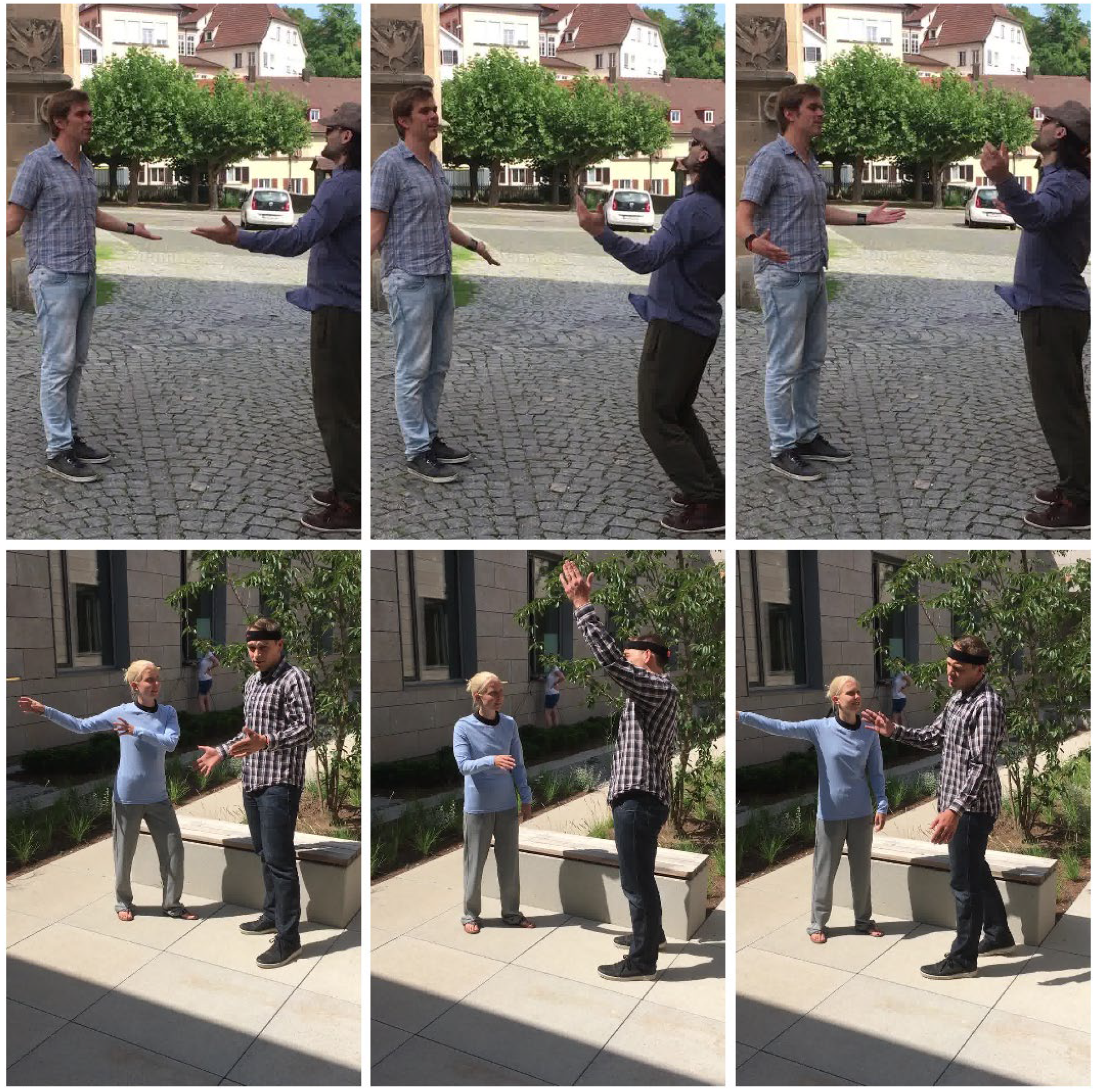
For this study, two datasets from a paper on “3D Human Pose in The Wild Using IMUs and a Moving Camera” [30] were utilized. The images of the dataset were already filed in different folders, with each folder containing images of a specific behavior. Actors were instructed to perform various expressions for every specific behavior, and the images contained these interactions from start to finish. No further processing was required by us at this point. We relied on the OpenCV library for the image reading process and loaded them into memory using cv2.imread() function. OpenCV can handle various image formats such as JPG and PNG. If an image could not be read, OpenCV converts it to an empty list to avoid code errors. For our purposes, the folders/behaviors utilized were courtyard_arguing_00 and downtown_arguing_00 for the argumentative behaviors containing interactions between two individuals arguing with each other (Figure 1), and courtyard_warmWelcome_00 and courtyard_giveDirections_00 for the non-argumentative behaviors containing interactions between two individuals casually talking, greeting each other and giving directions (Figure 2).
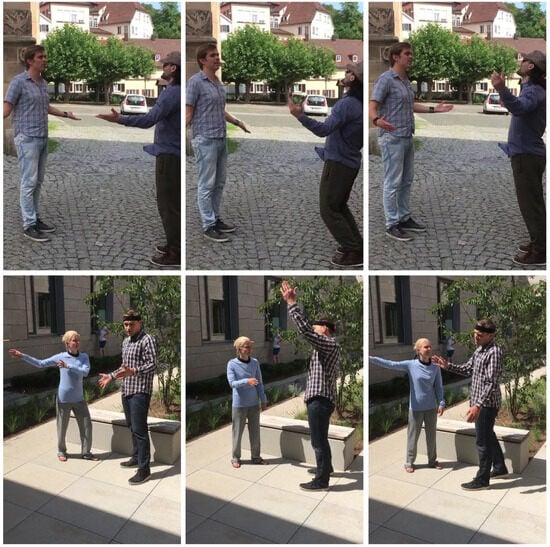
Figure 1.
Argumentative image dataset sample.
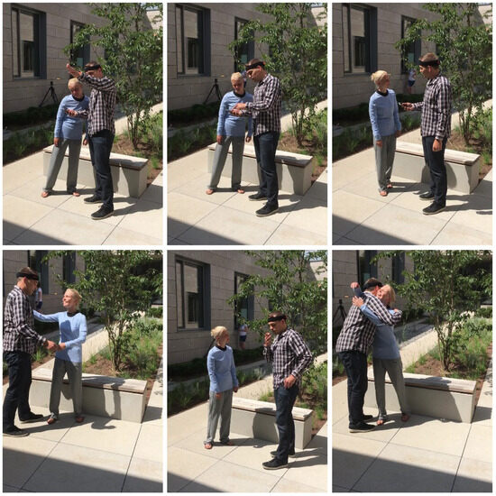
Figure 2.
Non-argumentative image dataset sample.
In this work, we defined a frame from the courtyard_arguing_00 or downtown_arguing_00 folder as a verbal-argumentative behavior, where the two individuals are having a verbal argument and disagree with each other using their hands, body and facial expressions to express their attitude. For non-argumentative behavior, we take frames from the courtyard_warmWelcome_00 and courtyard_giveDirections_00 folder, where the two individuals are casually discussing without expressing argumentative attitude.
- Argumentative Behavior Dataset: This dataset contains a combination of images from two different folders, courtyard_arguing_00 and downtown_arguing_00. Half of the images from each folder were used for training and the other half for testing. This includes images from two individuals in an argument that gradually escalated.
- Non-Argumentative Behavior Dataset: This dataset contains a combination of images from two different folders, courtyard_warmWelcome_00 and courtyard_giveDirections_00. Half of the images were used for training, and the other half for testing. This included images of two individuals in a warm greeting and giving directions to a specific destination.
- Number of Argumentative Images for training: 466 images;
- Number of Non-Argumentative Images for training: 466 images;
- Number of Argumentative Images for testing: 498 images;
- Number of Non-Argumentative Images for testing: 498 images.
2.2. Handling the Missing Data
Following image processing, landmarks with their corresponding coordinates for each frame were extracted into a single dataset (landmarks_data.csv). Each column represents coordinates of a value (x, y or z) for a specific landmark, and each row corresponds to a specific image. Moreover, a final column was added for classification labeling (1 marking the argumentative class and 0 the non-argumentative class).
As mentioned in Section 2.1, in case of a failed detection, landmarks, and therefore coordinates, were left empty. KNN imputation method was replaced by simple imputation in order to avoid overfitting and underfitting issues [31]. Taking the small size of the datasets used into account, simple imputation provided a more consistent bias by replacing missing values with a constant, whereas the KNN imputer may have introduced noise due to the fact that it relies on nearest neighbors, and therefore not true to the actual values. The number of images was divided equally for each class during training in order to avoid data imbalance. A simple imputer can easily manage imbalanced data, whereas KNN relies solely on equal data distribution among classes. Further, simple imputation can be beneficial in the case of the Random Forest Classifier and Gradient Booster because they are inherently robust to noise thanks to their ensemble nature. Therefore, overfitting can be avoided, as the simple imputer minimally affects the bias of the model. This means that the model’s performance remains unaffected, while the KNN imputer could introduce patterns to the Random Forest classifier and Gradient Booster leading to potential overfitting.
2.3. Artifact and Noise Management
In order to ensure the quality of the data, we applied noise reduction and quality control implementation [32,33] for a proper model validation.
- Noise Reduction Techniques
Right before the image processing, the code inspects the resolution of each image. If any image is below the defined resolution (640 × 480 pixels), then this image is skipped. This prevents the negative impact of low-quality or overly compressed images on landmark detection. Also, this ensures that the model will be provided with enough detailed images for accurate landmark detection. This Noise reduction technique aims to improve the clarity of the images given as the input right before the landmark extraction. We also used OpenCV’s fast non-local means denoising algorithm, to enhance the quality of the images for a more accurate landmark extraction from MediaPipe.
- Quality Control
The application of fast Non-Local Means Denoising using OpenCV’s cv2.fastNLMeansDenoisingColored() method in the code reduces noise in images while at the same time preserving important features like edges. The denoising parameters chosen were (10, 10, 7, 21), with the first two being responsible for controlling the noise filter strength for luminance and color channels. The other two parameters were responsible for fine-tuning the window size of the filter and its strength. This crucial step ensures that compression and noise artifacts in images will not negatively affect the process of the landmark detection, and therefore, the model can better capture the image features.
2.4. Extraction of Features Using MediaPipe
The method used for model development is the MediaPipe Holistic model for facial, hand gesture and body pose feature extraction. This model provides a robust landmark set. For each image, MediaPipe processes, detects and draws the following landmarks:
- Arms Gestures: A set of 21 landmarks for each hand corresponding to key points for it with proper x, y, z coordinates. These landmarks capture the positioning of fingers and the hand motions;
- Body Pose: A set of 33 landmarks for the body stance corresponding to key points for it with proper x, y, z coordinates. These landmarks capture the skeleton of the body providing a full-body pose estimation;
- Facial Features: A set of 468 landmarks for the face corresponding to key points for it with proper x, y, z coordinates. These landmarks capture facial expressions and can be relevant in expressions of feelings such as aggression.
This coverage gives us the ability to analyze hand gestures, body posture and facial expression simultaneously, which is crucial for classifying and detecting different emotions and behaviors. For proper model training, landmark extraction for each image was performed by combining them into a single feature vector containing the following:
- 63 + 63 values for each arm landmarks (21 landmarks for each hand multiplied by the count of coordinates [x, y, z]);
- 99 values for the body pose landmarks (33 landmarks for body stance multiplied by the count of coordinates [x, y, z]);
- 1404 values for the facial expressions landmarks (468 landmarks for body stance multiplied by the count of coordinates [x, y, z]).
The process for landmark extraction was as follows:
- The image file was first converted to RGB from BGR, which is the default format for OpenCV, since MediaPipe expects an RGB image as the input;
- The model then processes the converted images in order to detect and return the landmarks for the body pose, hands and face;
- If failure for landmark detection occurs, then NaN values are assigned to the list for the specific parts.
In order to successfully detect human behaviors, we prioritized specific essential components for our model. Our aim was to classify argumentative and non-argumentative behaviors, and therefore, we chose specific expressions and motions on the target behaviors. By prioritizing facial landmarks, emotions such as fear, sadness or anger can be indicated. Body language also can indicate such emotions based on the torso posture or the curve of the spine. Hands gestures are often used to express our feelings, such as dominance in a situation or disapproval. The choice of the selected features aligns with the existing literature [34,35] on behavioral analysis. This emphasizes the significance of interpreting human emotions based on the selected features.
2.5. Model Development and Training
In order to evaluate the efficacy of the chosen landmarks we extracted earlier, we chose three classification models: Random Forest, Gradient Boosting and Ridge Classifier. For accurate testing, we compared the performance of three state-of-the-art models in the field, and we utilized cross-validation metrics, t-paired testing for statistical comparison of our model superiority, F1 scores, accuracy, precision, recall, and confusion matrices.
- Random Forest Classifier: A commonly used machine learning algorithm that combines the output of multiple decision trees to reach a single result.
- Gradient Boosting: A technique based on functional space boosting. It gives a prediction model which contains an ensemble of weak prediction models. These models make very few assumptions about the data, in which most of the cases are simple decision trees.
- Ridge Classifier: A machine learning algorithm designed for multi-class classification tasks.
The test–train split technique was applied in our dataset, with 80% of the data used for training, and 20% of the data used for testing. In order to handle missing values in our model, we used the mean imputation strategy provided by the simple imputer. Next, we performed a cross-validation for the three classification models using 5 folds to evaluate the models’ performance and choose the model with the best performance ratio to advance.
2.6. Trained Model Evaluation
During training and cross-validation, the calculation and plotting of metrics was performed to assess each model’s performance.
- Accuracy: The percentage of the correctly classified samples.
- Precision: The percentage of true positives out of all positive classifications.
- Recall: The percentage of true positives out of all actual positive classifications.
- F1 Score: Harmonic mean of precision and recall.
- ROC Curve and AUC: A graphical representation of the trade-off between the true positive rate and false positive rate at various thresholds. They are used as a model’s ability to discriminate between classes.
- Confusion Matrix: The number of true-negative, true-positive, false-negative and false-positive classifications of the model.
- Learning Curves: A graphical representation of the model’s performance on the training and validation datasets over time. This graph represents the model’s accuracy or loss during training.
All metrics above were calculated for each model. Learning curves for each model displayed training and cross-validation scores against the number of training examples, providing an estimate of whether the model was overfitting or underfitting. The best model was selected based on the F1 score criteria.
2.7. Testing Model’s Performance on New Data
Before testing our model, it would be a good strategy to perform the fine-tuning of hyperparameters using GridsearchCV [36]. However, fine-tuning could sometimes lead to poor performance or in our case false predictions, as already happened in our initial model. The specific problems that were identified in the initial model using fine-tuning are as follows:
- Hyperparameters over-tuned to the validation set, especially in cases when the validation set is small, leading to false predictions on the test set;
- Dimensionality Curse [37]: Using the gridsearch method with many hyperparameters sometimes finds a good combination by chance, rather than through true model improvement;
- Ignored Shifts in Data Distribution [38]: In our case, as the validation set’s distribution is different from the test set, fine-tuning may produce biased hyperparameters, causing poor performance on the test set.
Thus, in this model, fine-tuning was entirely omitted. For model testing, a new set of images was utilized and fed to the best-performing model selected in the previous step.
- Model testing was performed through the classification of an argument between two individuals by using the second half of the images from the folders courtyard_arguing_00 and downtown_arguing_00. The total number of images in this class is 498.
- Casual conversation classification was performed by using images between two individuals casually chatting. The second half of the images from the folders courtyard_warmWeclome_00 and courtyard_giveDirections_00 were used. The total number of the images for this class is also 498.
2.8. Final Model Evaluation
The final results from the model prediction and probabilities were saved in a .csv file (detection_results.csv) for future analysis. Also, additional metrics, such as the total correct probabilities for argumentative and non-argumentative detections, were displayed and plotted. This included the probability for each separate detection, total F1 score, Accuracy, precision, recall, confusion matrices, ROC curves/AUC and positive and negative predictive values (NPV and PPV). These metrics provide a fine-grained understanding of the model’s classification capacity.
3. Results
During the evaluation of our three models, each model’s performance was calculated using cross-validation on the training data and with the help of evaluation metrics such as accuracy, precision, recall and F1 score.
3.1. Trained Model Performance
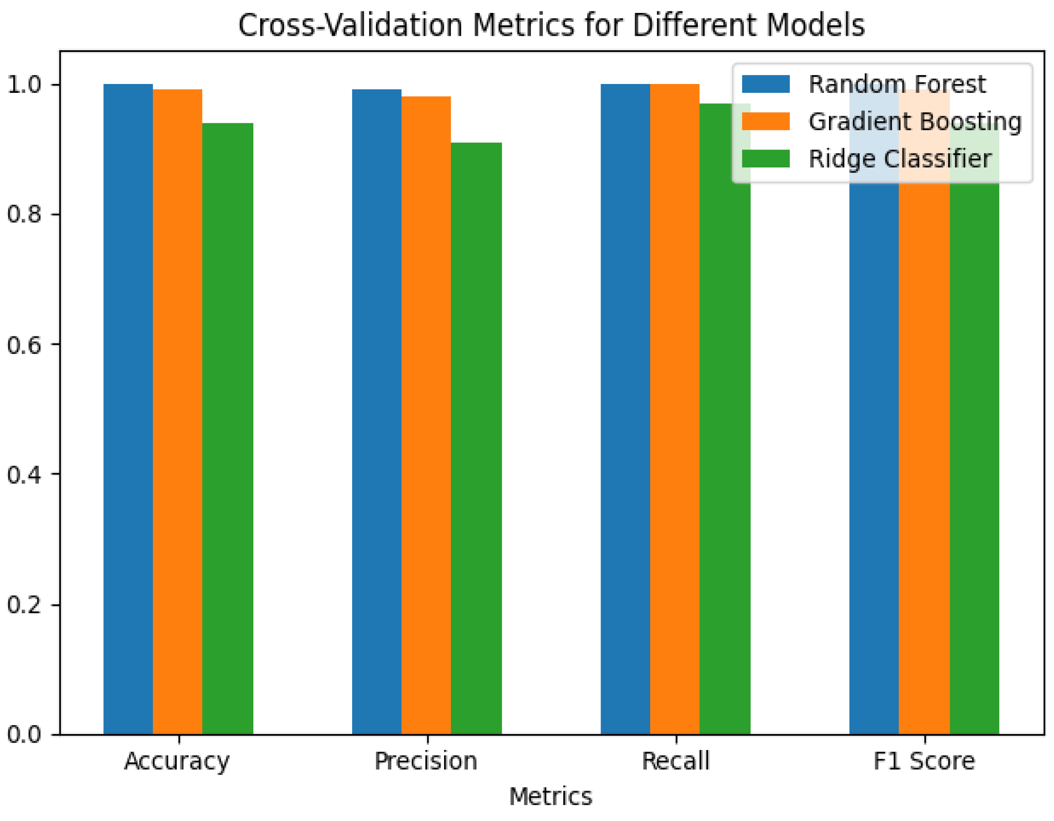
The best model in our case was considered the model with the highest F1 score. Cross-validation was limited to 5 folds in order to avoid overfitting issues and to correctly calculate each model’s general performance. The results are as shown in Table 1 and Table 2 and in Figure 3:
Random Forest Cross-Validation Metrics:
Accuracy: 1.00 (+/−0.01);
Precision: 0.99 (+/−0.02);
Recall: 1.00 (+/−0.00);
F1 Score: 1.00 (+/−0.01).
Gradient Boosting Cross-Validation Metrics:
Accuracy: 0.99 (+/−0.02);
Precision: 0.98 (+/−0.04);
Recall: 1.00 (+/−0.01);
F1 Score: 0.99 (+/−0.02).
Ridge Classifier Cross-Validation Metrics:
Accuracy: 0.94 (+/−0.05);
Precision: 0.91 (+/−0.06);
Recall: 0.97 (+/−0.05);
F1 Score: 0.94 (+/−0.05).
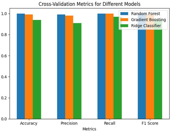
Figure 3.
Cross-validation metrics for the three models.
Figure 3.
Cross-validation metrics for the three models.
Even though the Gradient Boosting performance was exemplary, with similar results to the Random Forest Classifier, the preferred model was Random Forest due to its higher F1 score. Random forest exhibits a better balance between precision and recall making it more reliable. Also, Gradient boosting appears more likely to identify true positives, therefore maximizing recall with a cost in precision value. Following the best evaluated model selection (Random Forest), performance metrics were calculated using the test set as shown in Table 1.


Table 1.
Performance of the Random Forest classification model.
Table 1.
Performance of the Random Forest classification model.
| Precision | Recall | F1-Score | Support | |
|---|---|---|---|---|
| Class 0 (Non-Argumentative) | 1.00 | 1.00 | 1.00 | 89 |
| Class 1 (Argumentative) | 1.00 | 1.00 | 1.00 | 98 |
| Accuracy | 1.00 | 187 | ||
| Macro avg | 1.00 | 1.00 | 1.00 | 187 |
| Weighted avg | 1.00 | 1.00 | 1.00 | 187 |
Classification Performance on Test Set using Random Forest:
The Random Forest classifier exhibits excellent performance on the test set, with nearly perfect scores in all metrics [39]. The Test-Set Final Random Forest Cross-Validation Metrics are shown in Table 2.


Table 2.
Cross-validation evaluation metrics.
Table 2.
Cross-validation evaluation metrics.
| Metric | Value |
|---|---|
| Accuracy | 1.00 |
| Precision | 1.00 |
| Recall | 1.00 |
| F1-Score | 1.00 |
In addition, this high level of performance could indicate that the specific dataset used for this method aids towards developing this classifier and also that the dataset provides clear distinction between classes. As stated previously, methods preventing potential overfitting were used such as avoiding wrong imputation methods, advanced hyperparameter fine-tuning and unbalanced dataset usage. However, the final results could indicate possible overfitting. To mitigate this, cross-validation was used. Nonetheless, the derived classification model should be tested on different datasets, furthering the understanding of the model’s generalization [31]. Below are the learning curves for all three models, displaying performance and loss during training (see Figure 4).
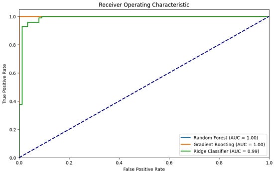
Figure 4.
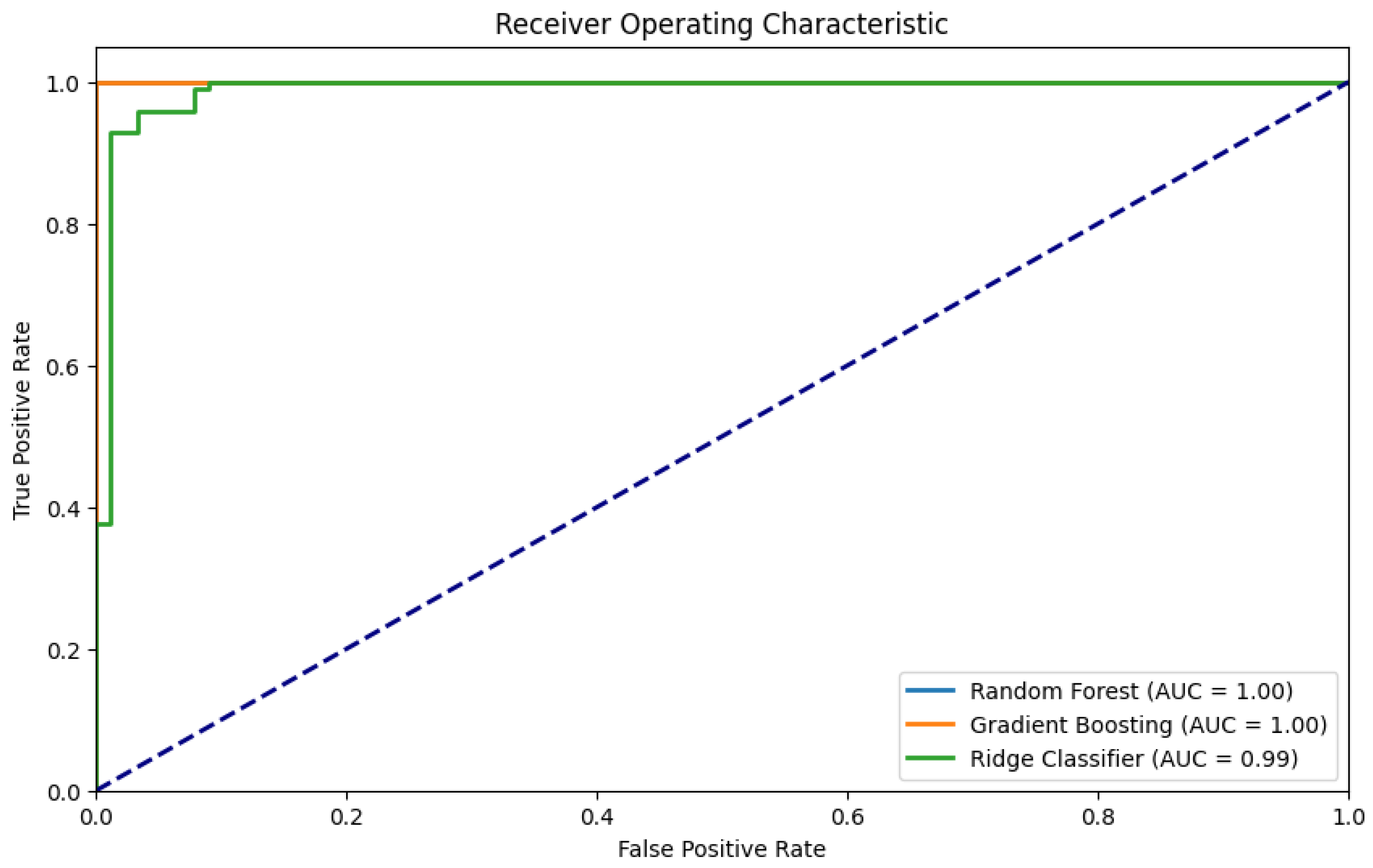
AUC scores of the three trained models. A model that makes random guesses (practically a model with no discriminative power), is represented by the diagonal dashed blue line that extends from the bottom left (0, 0) to the top right (1, 1). The ROC curve for any model that outperforms the random one will be above this diagonal line.
Random Forest and Gradient Boosting perform perfectly in classifying the positive and negative classes (Argumentative and Non-Argumentative), indicating that the model is able to identify all cases of argumentative and non-argumentative behaviors correctly and without errors. Ridge classifier’s AUC value of 0.99 is exceptionally high, showing that it is also performing with almost perfect accuracy.
Various techniques to control overfitting such as train–test split, cross-validation and confusion matrix evaluation are embedded in the code used to develop the models. The models display the ability to generalize effectively on the data based on the low standard deviations across the folds combined with the high performance metrics. However, in the presence of a potential overfitting risk due to the controlled setting of the dataset used, there is still the need to address some cases which may not be representative of a more diverse real-world scenario.
General Potential Risk Areas for Overfitting:
- Feature Engineering: The extraction of high-quality landmarks from the images serve as features for the model. If too-specific details are being captured from these features, the model could overfit to the specific data and may not be able to generalize to new data.
- Clean Dataset and High Performance: The dataset used for this model was within a sterile environment without much noise or artifacts. Despite this being a good case for our model training, leading it to perform exceptionally, it may cause it to perform less efficiently in real-world scenarios.
Gradient Boosting and Random Forest achieve high performance metrics for F1 score, recall, precision and accuracy. Their ensemble nature that combines multiple decision trees makes them generally robust to overfitting [40,41]. However, it is crucial to control overfitting and ensure that metrics are not misleading. In order to control overfitting, we included the following methods:
Imputation of Missing Values:
By handling missing values with simple imputation, we ensure that in cases of rows with incomplete data, the model does not overfit by discarding them entirely. The model is learning not just by one full row but from the entire dataset.
Training–Testing Split:
- The code splits the dataset into 80% of the data for training and 20% of the data for testing. Since the models are being trained on the training set and then evaluated on the test set that contains data unseen by the model during training, the performance results give a clear indication for a good model generalization.
- The performance metrics on the test are also very high (see Table 2), suggesting that the model learned meaningful patterns rather than memorizing data from training. If a significant performance drop had occurred on the test set, then it would be an indication of overfitting. In our case, the model does not exhibit such behaviors.
Cross-Validation:
- We performed 5-fold cross-validation during our model’s evaluation process. This technique is effective in controlling overfitting since it ensures that the model training is being evaluated on multiple subsets of the dataset, exposing it to different distributions of data. This prevents the model from memorizing patterns in a single set of training data.
- Also, the evaluation metrics (F1 score, recall, precision and accuracy) are averaged across the validation folds with their standard deviations being reported, indicating how much variance in performance happened across different folds, thus providing insight into the consistency of the model’s predictions across various data splits. High variance indicates potential overfitting. In our case, the low values on standard deviations suggest stable performance.
- The results for each model after cross-validation are very similar, indicating that the performance is good across all the different folds of the data, which is a sign of avoiding overfitting.
Further, the use of hyperparameter fine-tuning could help avoid overfitting in the future on a more complex dataset with higher levels of noise and artifacts. However, in our case, the hyperparameter tuning led to low ROC AUC scores and prediction accuracy, and was therefore omitted, as discussed later in the Section 3.3. L1 and L2 regularization techniques [42] prevent overfitting by discouraging the model of relying on a single feature by adding penalties to its complexity. Gradient Boosting and Random Forest are inherently resistant to overfitting due to their high performance in the generalization of the data, making the use of this technique not necessary in this case.
Proceeding with the model evaluation, the confusion matrices are displayed below for each method:
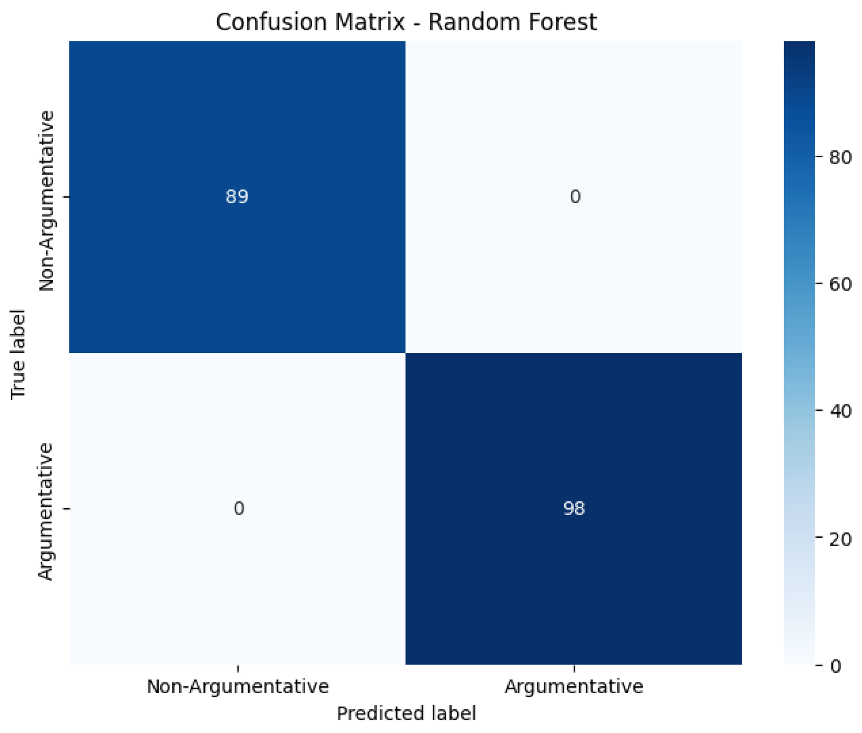
Random Forest Classifier (Figure 5)
True Positives (TPs): 98—Instances of the positive class correctly identified by the model.
True Negatives (TNs): 89—Instances of the negative class correctly identified by the model.
False Positives (FPs): 0—Instances of the negative class incorrectly identified by the model.
False Negatives (FNs): 0—Instances of the positive class incorrectly identified by the model.
Positive Predictive Value (PPV) for Random Forest: 1.0, meaning that during the prediction of a positive instance, the Random Forest is correct 100% of the time.
Negative Predictive Value (NPV) for Random Forest: 1.00, meaning that during the prediction of a negative instance, the Random Forest is correct 100% of the time.

Figure 5.
Confusion matrix of Random Forest Classifier after training.
Figure 5.
Confusion matrix of Random Forest Classifier after training.
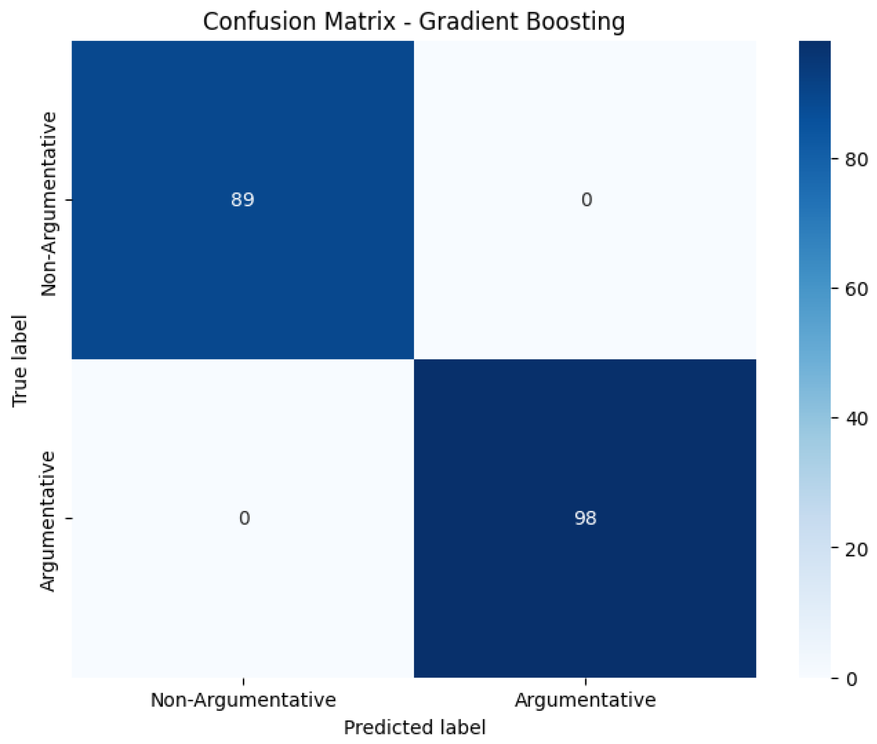
Gradient Boosting (Figure 6)
True Positives (TPs): 98—Instances of the positive class correctly identified by the model.
True Negatives (TNs): 89—Instances of the negative class correctly identified by the model.
False Positives (FPs): 0—Instances of the negative class incorrectly identified by the model.
False Negatives (FNs): 0—Instances of the positive class incorrectly identified by the model.
Positive Predictive Value (PPV) for Gradient Boosting: 1.0, meaning that during the prediction of a positive instance, the Random Forest is correct 100% of the time.
Negative Predictive Value (NPV) for Gradient Boosting: 1.00, Meaning that during the prediction of a negative instance, the Random Forest is correct 100% of the time.
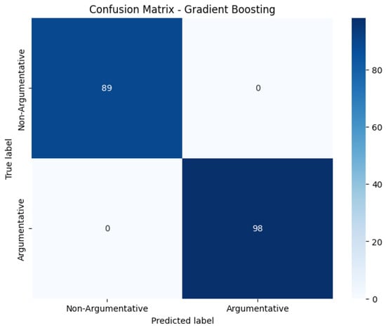
Figure 6.
Confusion matrix of Gradient Boosting after training.
Figure 6.
Confusion matrix of Gradient Boosting after training.
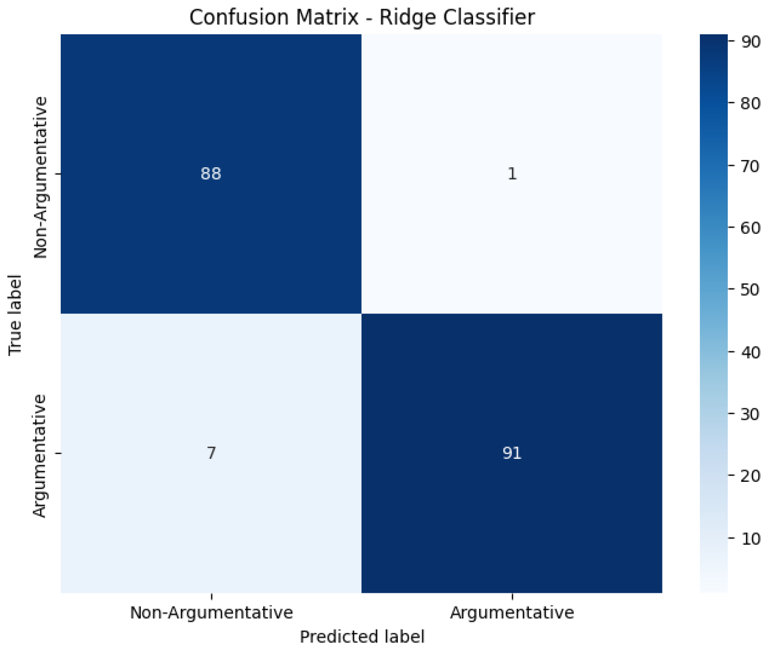
Ridge Classifier (Figure 7)
True Positives (TPs): 91—Instances of the positive class correctly identified by the model.
True Negatives (TNs): 88—Instances of the negative class correctly identified by the model.
False Positives (FPs): 1—Instances of the negative class incorrectly identified by the model.
False Negatives (FNs): 7—Instances of the positive class incorrectly identified by the model.
Positive Predictive Value (PPV) for Ridge Classifier: 0.99, meaning that during the prediction of a positive instance, the Random Forest is correct 99% of the time.
Negative Predictive Value (NPV) for Ridge Classifier: 0.93: Meaning that during the prediction of a negative instance, the Random Forest is correct 93% of the time.
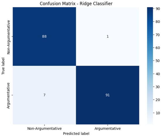
Figure 7.
Confusion matrix of Ridge Classifier after training.
Figure 7.
Confusion matrix of Ridge Classifier after training.
Both Random Forest classifier and Gradient Boosting performed exceptionally well, both outperforming Ridge Classifier with no false positives. This resulted in perfect PPV and NPV scores. Confusion matrices indicate that Gradient Boosting and Random Forest perform better than Ridge Classifier, taking precision and overall prediction accuracy into account. The Ridge Classifier has a lower accuracy than the previous two, with PPV and NPV values also lower when compared to the ensemble methods. This concludes that Ridge Classifier struggles with distinguishing between classes and is therefore less reliable. Depicted below are the learning curves of the machine learning model’s performance over time. Below we present the results of the learning curves from all three classification models during training.
Random Forest Classifier:
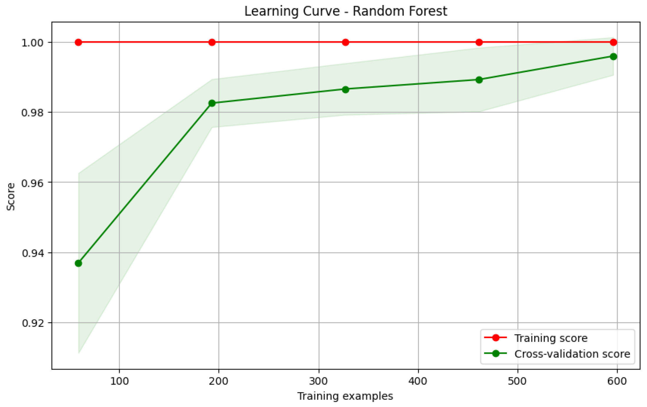
Training score: Depicts the performance of the model during its training with the training dataset. Random forest classifier shows that the model is fitting very well the training data (Figure 8).
Cross validation score: This curve depicts the performance of the model during training using a validation or test set unknown to the model and therefore showing how well the model generalizes unseen data. Random forest classifier shows an incremental cross-validation score from the beginning until 200 samples and then follows a slow but steady incremental course, reaching its peak near 600 images. This indicates the high data suitability of the dataset used since the cross-validation score almost meets with the training score (see Figure 8).
Figure 8.
Learning curve of Random Forest Classifier after training.
Figure 8.
Learning curve of Random Forest Classifier after training.
Gradient Boosting:
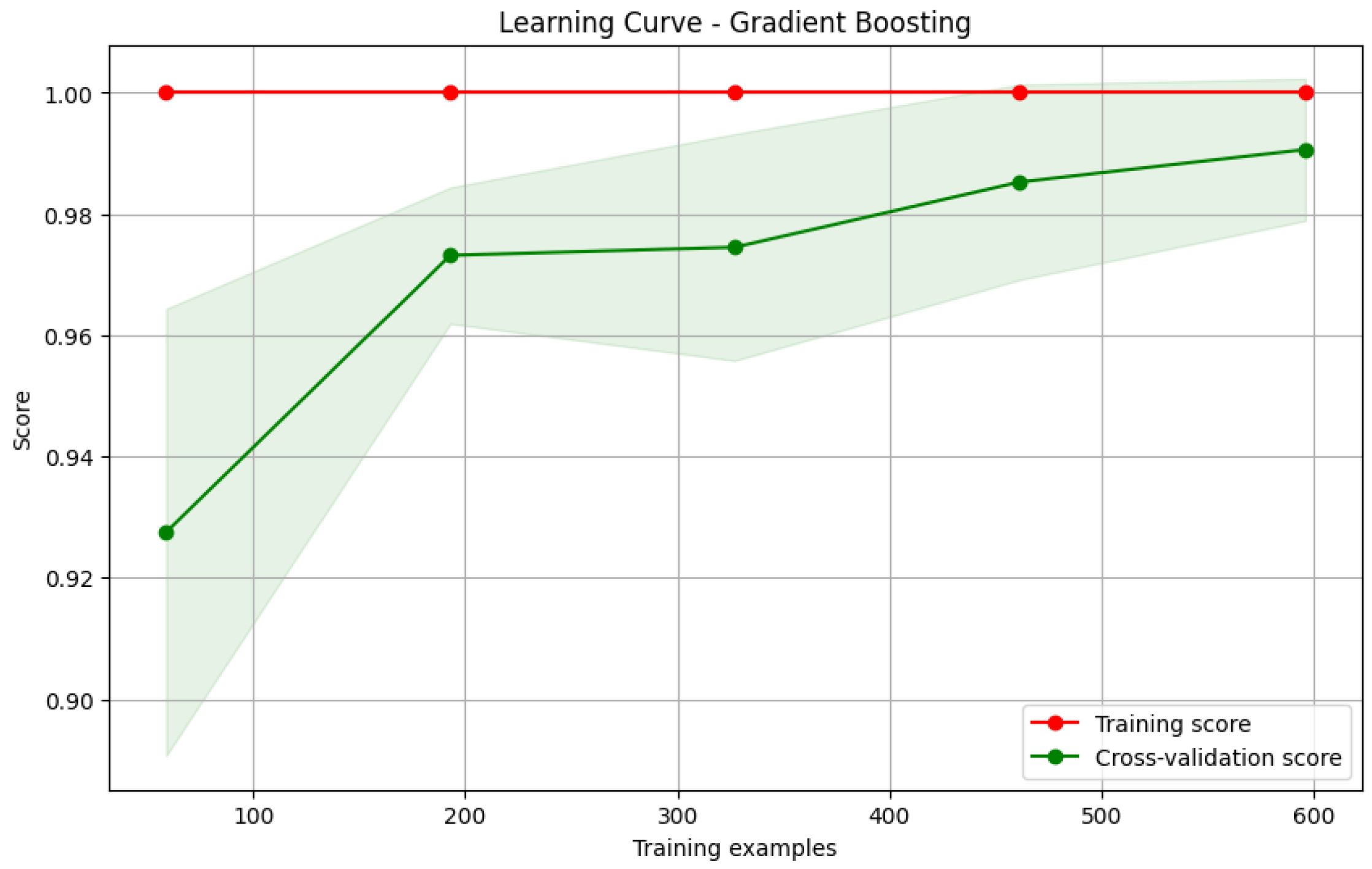
Training score: Gradient boosting also shows that the model is fitting very well the training data (Figure 9).
Cross-validation score: The learning curve for Gradient boosting indicates an initial steep rise during training until 200 samples, then an almost steady learning curve in the region of 200 and 320 samples, and then a further incremental way from 320 to 600 samples, indicating that sample numbers of around 350 and 600 are suitable for this model (Figure 9). Gradient Boosting shows a similar learning curve with Random Forest with the cross-validation score almost meeting the training score but with a higher divergence.
Figure 9.
Learning curve for Gradient Boosting after training.
Figure 9.
Learning curve for Gradient Boosting after training.
Ridge Classifier:
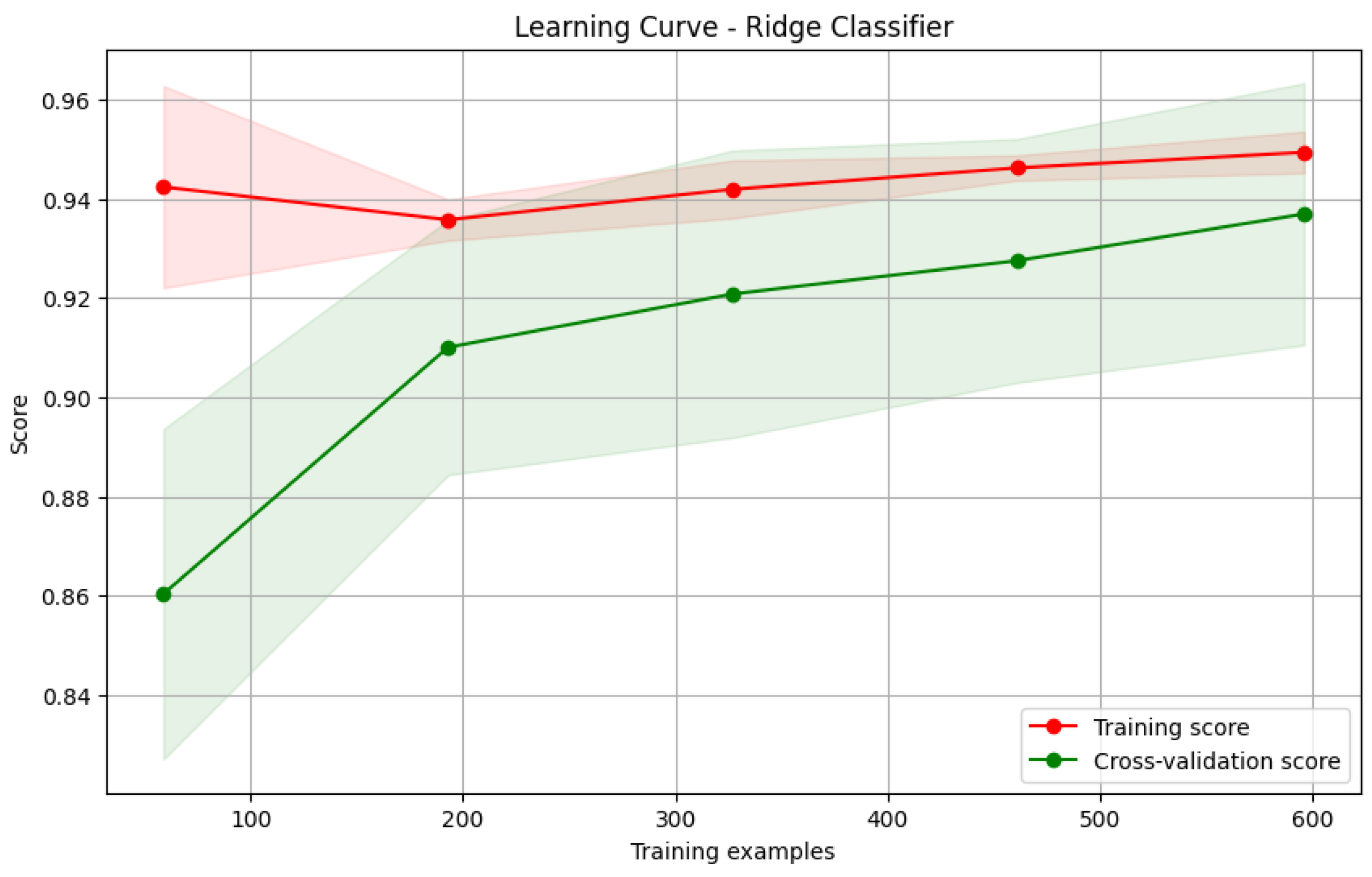
Training score: Finally, Ridge Classifier shows inferior data fitting starting at 0.94 while decreasing around the 200 samples and then steadily increasing again until 600 samples were used (Figure 10).
Cross-validation score: Despite the poor data fitting, the learning curve steadily increases from around 200 samples to the point of 600 samples, where the cross-validation score data tries to meet the training score (Figure 10).
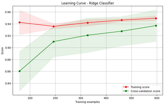
Figure 10.
Learning curve of Ridge Classifier after training.
Figure 10.
Learning curve of Ridge Classifier after training.
Since cross-validation alone is insufficient to confirm the superiority of our models, we used the paired t-test technique [43] for each of our models on the cross-validation results in order to determine if there were statistically significant differences. Following cross-validation, metrics (accuracy, precision, F1 and recall) from all models were compared. The result provided a t-statistic and p-value. For a statistically significant difference between our three models, the p-value should be less than 0.05. A greater t-statistic value indicates a more significant difference in model performance. A statistically significant difference is considered a t-statistic value larger than 2 or less than −2.
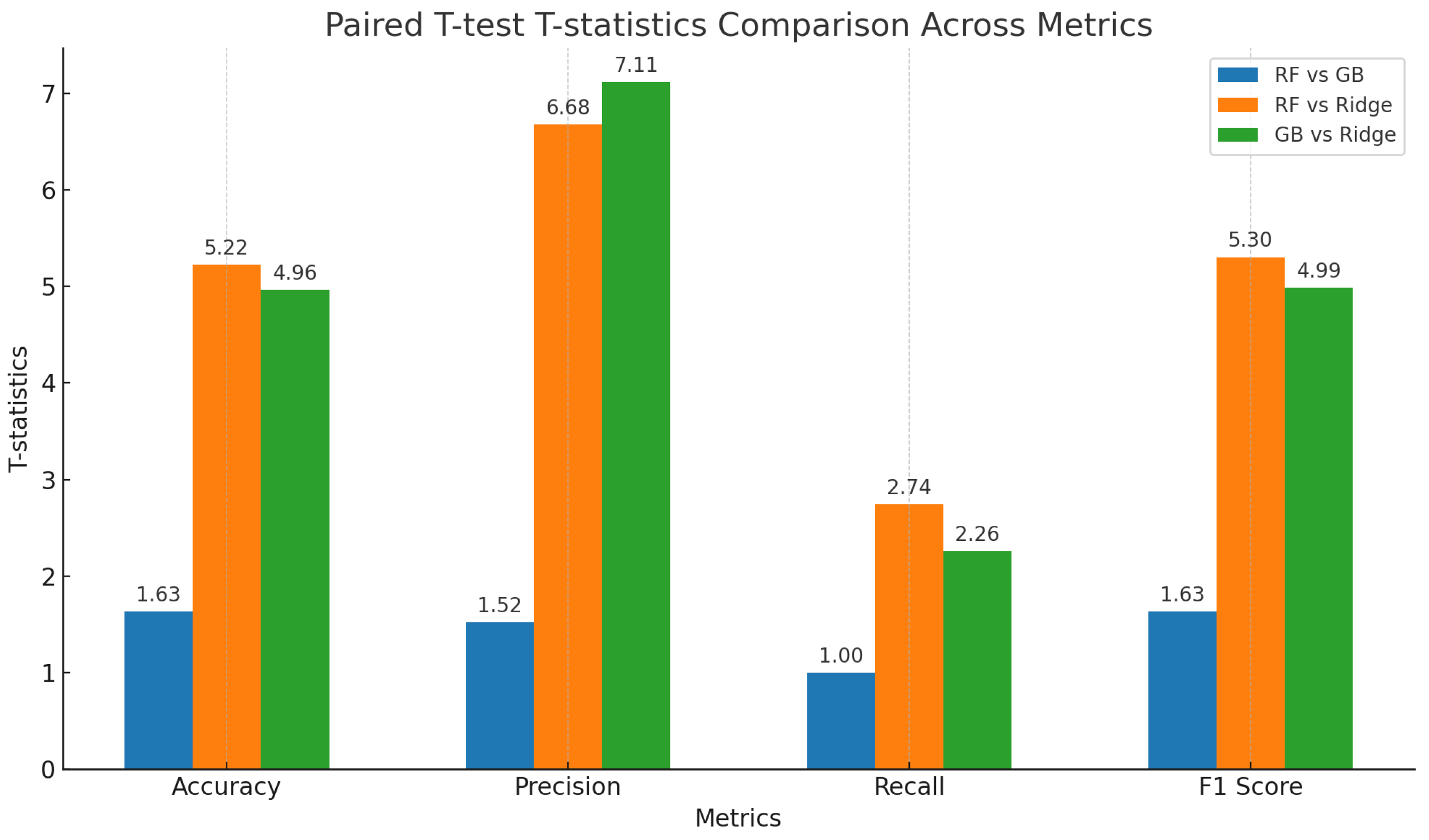
As seen in Figure 11, we performed paired t-tests on our models for all their metrics and evaluated the relative performance. The results were inherently paired since the models were assessed and trained on identical cross-validation splits, which is why the paired t-test was selected.

Figure 11.
Paired t-test statistic results across all models and metrics.
F1 Score: No significant difference was found between Random Forest and Gradient Boosting with t = 1.633 and p = 0.178. Random Forest outperformed Ridge Classifier with t = 5.302 and p = 0.006. Similarly, Gradient Boosting outperformed Ridge Classifier with t = 4.986 and p = 0.008.
Recall: In this metric, the results suggest that all models performed similarly in terms of recall, with the comparison between Random Forest and Gradient Boosting being t = 1.000 and p = 0.374. Similarly, between Random Forest and Ridge Classifier the difference was t = 2.743 and p = 0.052. Finally, Between Gradient Boosting and Ridge Classifier the significant differences were negligible with t = 2.260 and p = 0.087.
Precision: No statistically significant difference was shown between Random Forest and Gradient Boosting with t = 1.521 and p = 0.203. However, Random Forest outperformed Ridge Classifier significantly with t = 6.678 and p = 0.003. Gradient Boosting also outperformed Ridge Classifier with t = 7.115 and p = 0.002.
Accuracy: Random Forest and Gradient Boosting comparison showed values of t-statistic = 1.633 and p = 0.178, indicating no statistical significance between these models. Comparing Random Forest and Ridge Classifier the difference was statistically significant with t = 5.222 and p = 0.006, indicating that Random Forest outperforms Ridge Classifier in accuracy. Similar results were found when comparing Gradient Boosting and Ridge Classifier with t = 4.961 and p = 0.008.
The t-test results in Table 3 show that Both Gradient Boosting and Random Forest models greatly outperformed the Ridge Classifier in terms of Accuracy, Precision and F1 score, producing statistically comparable outcomes across all metrics. No significant difference was found in the recall metric throughout the models. According to these results, Both Gradient Boosting and Random Forest present excellent choices for classification implementation in this situation.

Table 3.
Results of paired t-tests.
3.2. Final Model Performance
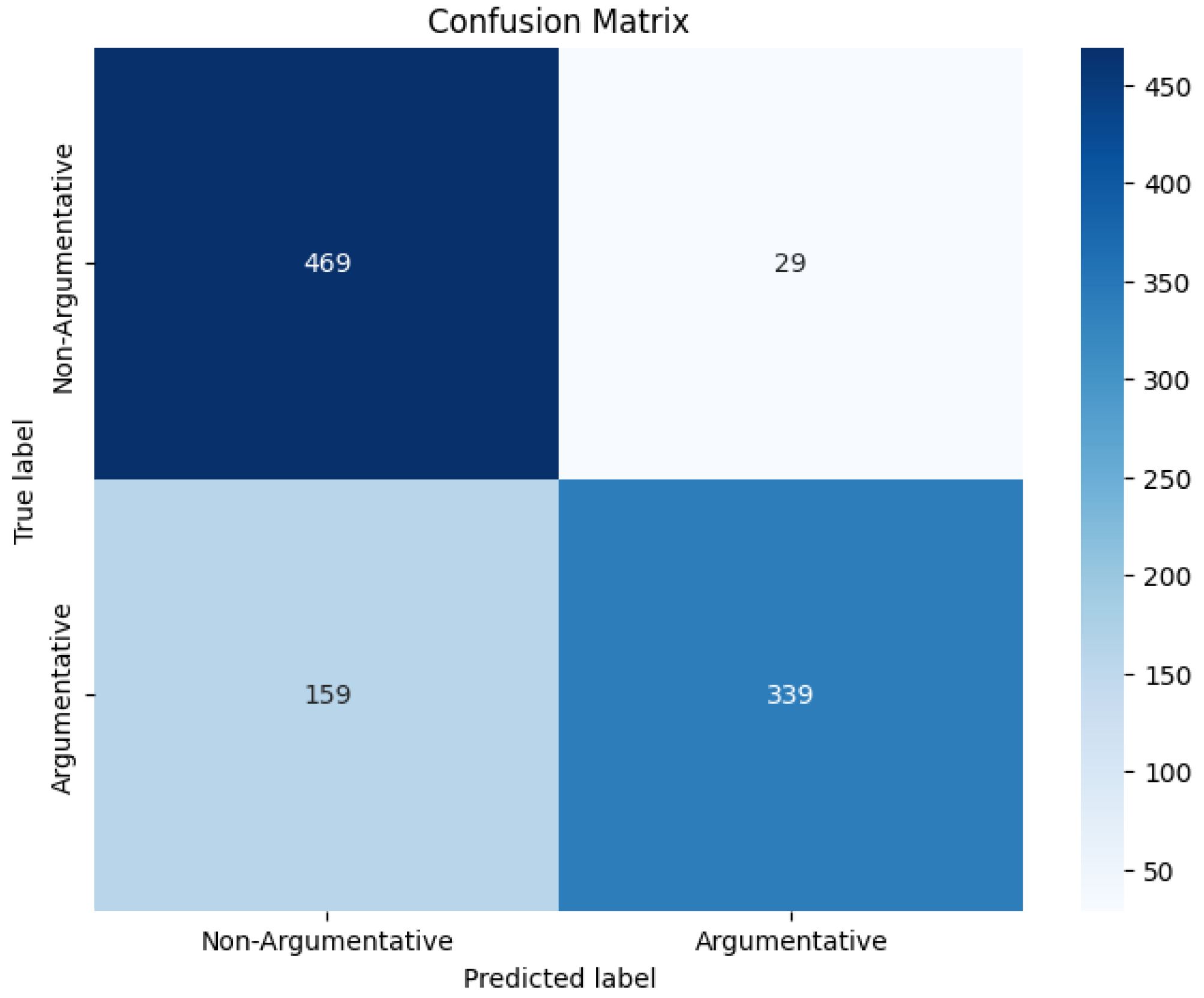
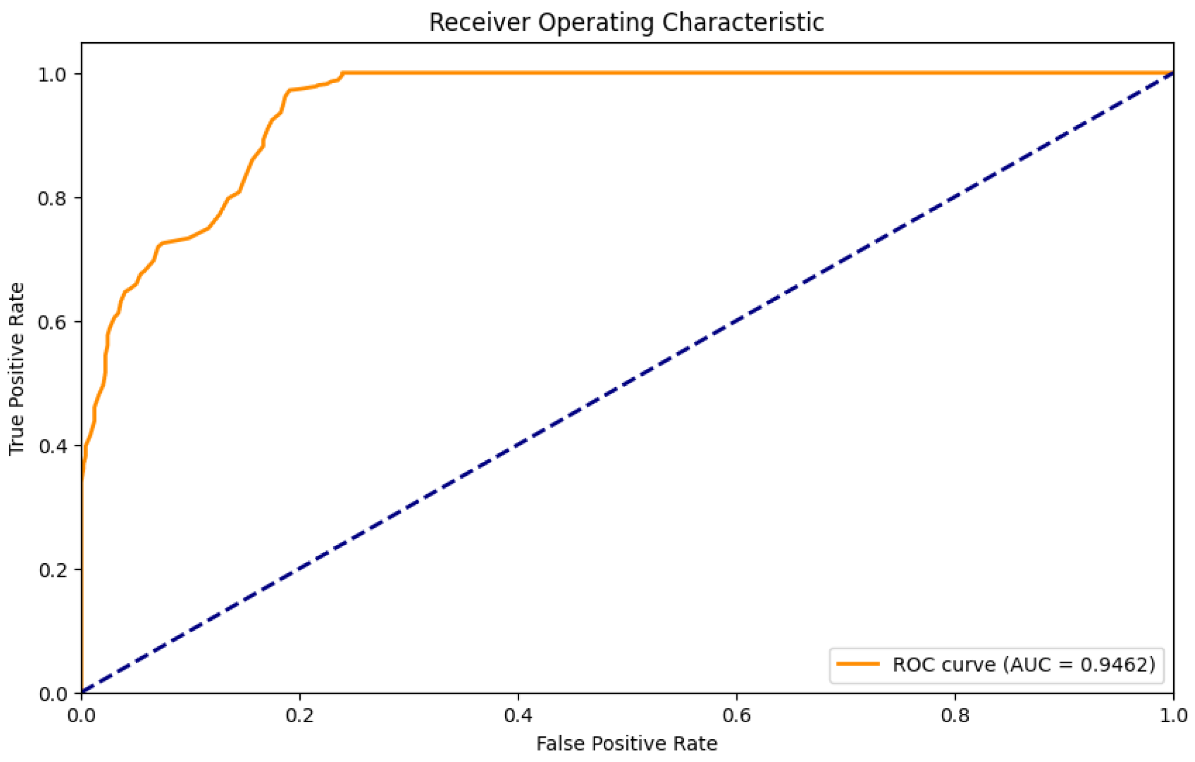
Following the training and model evaluation of the Random Forest Classifier, the pictures that remained unused during training were now used during testing in order to avoid misleading performance metrics, poor generalization and unreliable testing evaluation. By presenting new, unseen data in our model, we ensure its neutrality. The final results were derived after two separate folders were used, with two different classes of images, each with 498 images. Below, the results are presented, along with the confusion matrix in Figure 12 and ROC AUC scores in Figure 13.
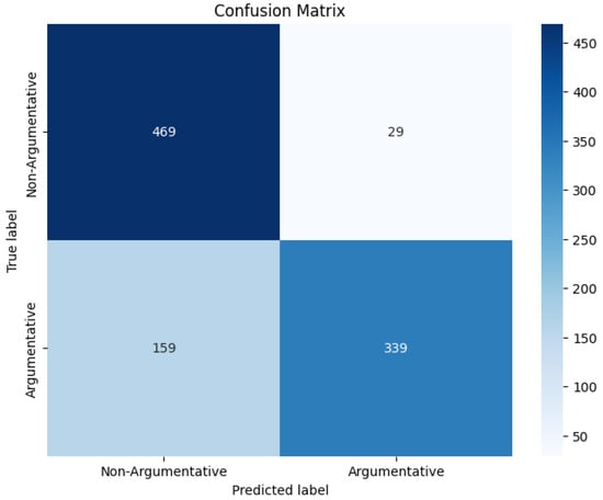
Figure 12.
Confusion Matrix of Random Forest Classifier after testing.
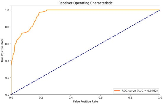
Figure 13.
ROC AUC score of Random Forest Classifier after testing.
Random Forest Final Evaluation Metrics after Testing:
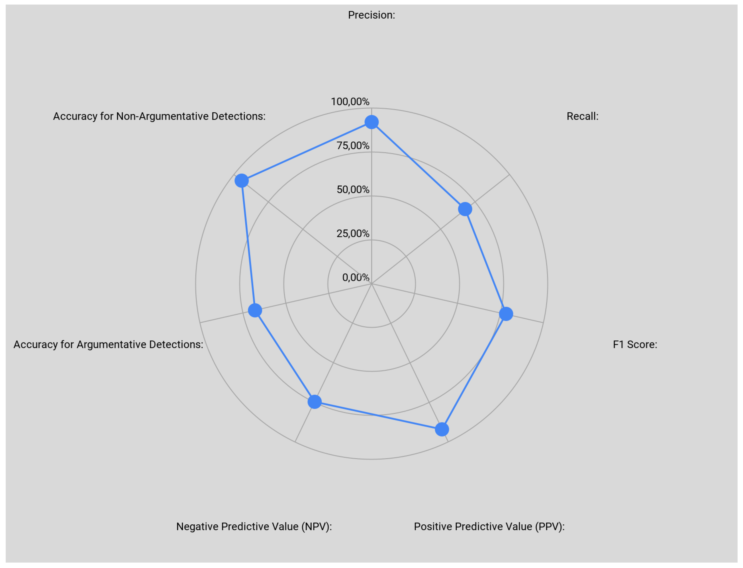
Accuracy: 81.12%
Correct classifications of the model during final testing correspond to a reasonably good performance considering the context of the dataset’s class distribution.
Precision: 92.12%
During the prediction of an argumentative or non-argumentative instance, the model had a 92.12% probability of correct classification. This suggests that the model is reliable in positive predictions with minimal numbers for false alarms.
Recall: 68.07%
From all the actual argumentative and non-argumentative instances, the model correctly identified 68.07% of the true instances. The remaining 31.93% of instances were false negatives.
F1 Score: 78.29%
This score reflects a good balance between recall and the precision scores of the model, also highlighting the potential for improvement.
Positive Predictive Value (PPV): 0.9212
This translates to the classification by the Random Forest model being correct 92% of the time.
Negative Predictive Value (NPV): 0.7468
The classification of a negative instance is correct 74% of the time.
True Positives (TPs): 339—Instances of the positive class correctly identified by the model.
True Negatives (TNs): 469—Instances of the negative class correctly identified by the model.
False Positives (FPs): 29—Instances of the negative class incorrectly identified by the model.
False Negatives (FNs): 159—Instances of the positive class incorrectly identified by the model.
Below are the final evaluation metrics of the final model after testing:
Accuracy for Argumentative Detections: 68.07%
From 498 images with true labels as argumentative, the model only identified 68.07% of them as actual argumentative.
Accuracy for Non-Argumentative Detections: 94.18%
From 498 images with true labels as non-argumentative, the model only identified 94.18% of them as actual non-argumentative.
The ROC curve in Figure 13 indicates that the model has excellent power for discriminating between different classes (in our case, argumentative and non-argumentative behaviors). The value of 0.9462 suggests that our model can distinguish between the two classes correctly 94.62% of the time. Further, this illustrates how the model performs at various decision thresholds. Moreover, a high AUC suggests that the performance of the model across different thresholds performs well, balancing FPR and TPR. Final results showcase a good prediction balance between two classes, falling between the 0.8–0.9 accuracy values. Values are based on the results derived as a direct output from our code after the testing finalization, saved in a ‘detection_results.csv’ file. Final results are shown in Figure 14 and Figure 15.
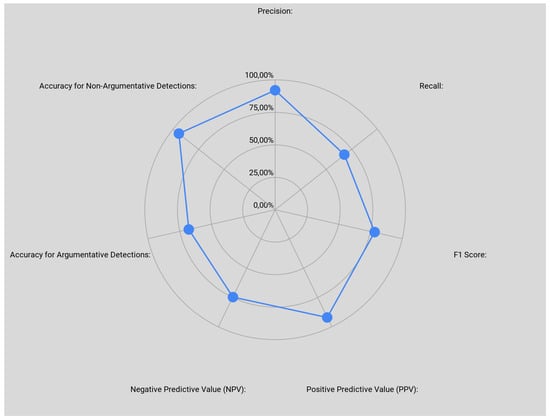
Figure 14.
Final model evaluation metrics.
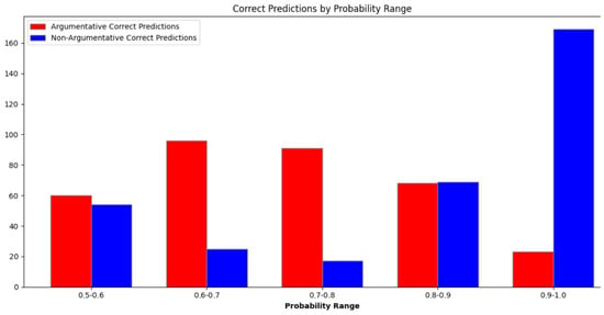
Figure 15.
Probability range/count of correct argumentative and non-argumentative predictions per 0.1 accuracy range, with 1.0 being the perfect accuracy score.
It is important to ensure that our model is both accurate and computationally efficient for real-time analysis. In order to address the computational efficiency and scalability of our model, we followed the implementation of measuring inference time [44] and evaluated its scalability using batch processing [45].
Inference Time Measurement:
- Timing Function: We used Python’s time module to accurately calculate inference times for our model on our dataset;
- Adding inference_times list: This allowed us to collect the times for each batch size;
- Timing the predictions: The time was recorded before and after the predictions to calculate the inference time;
- Saving times: The results were saved in a .csv file called inference_times.csv.
Scalability Evaluation with Batch Processing Usage:
- Parallelization: Using the joblib function, our model utilizes all available processing cores of the machine;
- Batch Processing: Implementation for inference to indicate how the model handles larger data sizes;
- Batch Size Evaluation: Evaluation through a loop for different batch sizes.
Interpretation of Results:
The results shown in Table 4 showcase inference times for different batch sizes. We measure in seconds the time the model needed to make predictions. The lower the times, the better the computation efficiency.

Table 4.
Results of inference times using batch processing.
High inference times are associated with smaller batch sizes. Comparing batch sizes of 5, 10 and 20, the time for batch size 1 is greater at 0.00572 for argumentative and 0.00397 for non-argumentative labels. This shows that the model is not that efficient on parallel computation when processing one image at a time.
A small variation in inference time when working with larger batch sizes is observed. The time increases negligibly as the batch size increases from 5 to 20 and even slightly decreases (batch size 5 is slightly faster than 1). This indicates the model’s ability to benefit from batch-level optimization and process multiple images at once.
For both argumentative and non-argumentative labels, the inference time per instance often drops with batch size. This indicates that the model can effectively handle larger datasets by processing multiple instances at once. For an argumentative label, the inference time at a batch size of one is 0.00572 s. For each instance, the time drops to 0.00352 s when the batch size is increased to 20.
The model’s results show that it can effectively scale when the batch size is increasing, while maintaining low inference times making it ideal for real-time clinical applications.
3.3. Secondary Analysis (Initial Model)
As we discussed earlier, our initial model utilized KNN imputation and fine-tuning the gridsearch using hyperparameters. Although these techniques were used to provide a more accurate and efficient model, the results showed potential overfitting/underfitting problems, and the final results indicated that the model was not capable of providing correct detections. Thus, this led us to redevelop the model with simple imputation instead of KNN imputation and without the use of hyperparameter fine-tuning. Below, we provide the results of the model during the training and testing phases. Figures S1–S16 are the results and metrics from our initial model.
The initial model displayed average to low accuracy 0.68 (almost based on random chance) with 0.85 precision, 0.45 recall and 0.58 F1 score, as shown in Table S3. It has also shown a low percentage of certainty for predicting the correct class and a high percentage of certainty for predicting the wrong class based on the true label. This indicated potential overfitting. We ruled out other factors that could have contributed to this poor performance, such as class or data imbalance, noise, outliers, incorrect labels and improper training [31]. Considering the fact that Gradient Boosting and Random Forest Classifier are both ensemble models and that KNN imputation along with fine-tuning could potentially create overfitting problems, since these models already have mechanisms that inherently help fine-tune the model by design, we decided to drop the initial model and redesign the new one by skipping fine-tuning and replacing KNN imputation with simple imputation.
4. Discussion
Patients with dementia can exhibit aggressive behaviors towards caregivers and mental health institutes, increasing the risk of harm to themselves and others. Various studies have examined the factors related to these behaviors. A primary focus is to assert the dangers of these behaviors thereby reducing stress to caregivers [16,18]. In order to better understand factors involved in agitation and aggressive behaviors in patients with dementia, further examination of the relationship between various types of behaviors has been undertaken by studying physically and verbally aggressive and non-aggressive behaviors. The results showed that the most disruptive type of aggression was verbal aggression [17].
Factors that cause aggressive behaviors and early signs that portend aggressive behavior in patients with dementia have previously been recognized. Hyperactivity, persecutory ideas and sad appearances can occur prior to an aggressive episode [8]. In emergency departments, dementia is a common condition among elderly patients. Patients exhibit psychotic symptoms, disturbances in motor activity and aggression. One study concluded that there are specific body movements from these patients anteceding an aggressive outburst [46].
Machine learning application approaches have been applied in psychiatry such as PTSD diagnosis [6], early stage dementia diagnosis and MCI, as well as First-Episode Psychosis using novel approaches such as multilayer perceptron and Support Vector [9,47]. Thus far, there are no studies in the field predicting aggressive behavior using machine learning models utilizing body pose and facial features expressions.
In this study, we developed, trained and validated a machine learning model that is capable of detecting and classifying argumentative and non-argumentative behaviors between two individuals in video frames. This foundational model is presented as a potential application for preventing aggressive outbursts in dementia patients. Limitations in acquiring datasets from dementia patients present a hurdle in the context of ethical concerns and patient consent. Collaborations with partners from the psychiatric section are needed in order to test this proof of concept model by obtaining access to clinical data from patients suffering from dementia. This will allow us to evaluate the model in real-world scenarios and enhance the robustness and reproducibility of our findings in subsequent research. The final model has high precision (90.18%) [39], translating to the high reliability of positive predictions and equal representation of classes in fair evaluation due to its balanced dataset. However, the model has a moderate recall (70.08%), a low NPV score (75.53%) and a substantial decrease in performance from training to testing. The reasons for the latter include overfitting or data discrepancies [31].
Among the strengths of our model are high classification metrics pointing to high effectiveness in distinguishing between two classes and its robustness to different operating conditions, performing well even under different decision thresholds (Figure 15) [39]. Further, the model exhibits high precision in positive predictions and can accurately distinguish the two separate classes of behaviors with false positive rates remaining low. Ensemble classification models (Random Forest Classifier/Gradient Boosting) are appropriate in order to avoid overfitting and thereby contribute to the overall performance of the model. Its adaptability to different operating conditions and consistent performance in various decision thresholds makes it a good launching pad for potential clinical applications in detecting and predicting aggressive behaviors in dementia patients, which could improve intervention strategies employed by caregivers and management.
Regarding the model’s weaknesses, these pertain mostly to the model’s metrics. A moderate recall score (70.08%) indicates false negative classification at a higher rate, which translates in some instances to argumentative behaviors not being identified. Moreover, low Negative Predictive Values scores (75.53%) indicate that the model has a lower predictive ability of non-argumentative behaviors and potentially misclassifies true negatives, as shown in Figure 15. Additionally, the model exhibits a performance drop from training to testing as shown in Figure 4 and Figure 13, correspondingly. This could be due to data discrepancies in the dataset used during training and testing, which attests to the need for further testing in real-world scenarios. The current dataset contains frames from verbal arguments and physical conversations. The controlled nature of the dataset could affect the model’s ability to perform well in real-world scenarios, and the use of clinical data may improve the model’s performance and its applicability in realistic conditions.
The choice of Random Forest, Gradient Boosting and Ridge Classifier was based on their computational efficiency for real-time clinical application, their robustness, efficiency and interpretability in handling complex characteristics, and their balancing accuracy, clinical relevance and resource efficiency. Nonetheless, models such as SVM or deep learning models were deemed less suitable due to difficulties with interpretability, their requirement for bigger datasets to work efficiently and their greater computational requirements. More specifically, Support Vector Machines rely on hyperplane separation and weight features, which conflict with the nature of coordinate-based data since all coordinates are needed to perform accurate detections and not weighted features. Also, Support Vector Machines have less interpretability, which is not suitable for clinical data. Deep learning also provides limited interpretability with difficulty in extracting meaningful patterns directly. Although they can theoretically capture complex dependencies, they require larger datasets in order to work correctly while needing high computational power [48,49].
Ethical Considerations
Considering the wider moral ramifications of machine learning algorithm application for predicting aggressive behaviors in vulnerable populations, we must address related ethical issues such as privacy and misclassification risk [50,51].
Privacy: Sensitive information is often included in predictive models such as video recordings, images, audio biometric data and behavioral logs. In order to avoid misuse or illegal use, we must therefore adhere to strict privacy laws and ethical norms. The anonymity of all datasets and participants is a critical part, and the individuals must be fully informed about the intended use of their data and provide their consent. Strict data protection is also a very important role of the researchers especially for vulnerable groups.
Risk of False Positives and False Negatives: Various consequences could result from false positives, such as unnecessary treatment or stigmatization due to inaccurate aggressive behavior prognostications. These may negatively affect the health of vulnerable patients or result in erroneous measures. Predictive models are employed as tools for supporting clinical decision making. The combination of machine learning with the expertise of trained staff can lead to the mitigation of such risks.
Bias and Fairness: Algorithms can apply biases in training data and cause the production of wrong results. This is especially problematic when working with communities or vulnerable populations. Mitigation strategies are included during the development of such models. Steps to ensure the bias reduction, fairness and transparency of such systems must be carried out regularly.
Ethical Deployment and Oversight: Engaging mental health and interdisciplinary teams of experts is crucial before implementing such models in community settings such as psychiatric hospitals, schools or prisons. The morality of these models must be guaranteed in order to avoid undue hazards to those who are already at risk.
Accountability and Human Agency: Machine learning models are meant to support human judgment. Experts able to comprehend the model’s behavior and predictions in the larger context should be responsible for case-by-case utilization. In order to assure such functionality, explicit accountability frameworks should be put in place when working with vulnerable populations.
5. Conclusions
In this study, the main goal was to create a robust model with high accuracy for detecting argumentative behaviors. This was achieved through testing different methodologies, classification models and approaches. The final model is a proof of concept that could be utilized in the future in a clinical setting for training based on frames and images from dementia patients, thus averting behavioral escalation which could potentially lead to an aggressive episode. The predictive model could therefore detect a patient’s combined facial features, body stance and hand gestures and prognosticate whether the behavior will escalate to an aggressive outburst. This could be beneficial both to patients and caregivers, enabling the effective management of such episodes. The performance of the model indicates that it is capable of accurately classifying the behavior of two individuals that are either in a verbal argument or a casual conversation. The dataset utilized in the model during training contained frames from videos that contained only arguments or a casual conversation. The evaluation of the model and its ability to correctly identify new unseen data shows promising results for a future work with clinical data of dementia patients, in order to perform predictions of an upcoming aggressive outburst and prevent it before the patient inflicts harm to him/herself or others.
It should also be taken into consideration that real-world data usually contain additional variability and noise. Even though this study focuses on a dataset in a controlled environment for argumentative and non-argumentative behaviors, real-world testing must take place in order to test the capabilities of our model further. Future work can broaden the model’s evaluation by incorporating acquired clinical data in real-world scenarios and increase the divergence of the classes. This will provide useful insights in evaluating model resilience in more realistic settings by encompassing a greater variety of noise levels and behaviors. It is also important to consider datasets containing a wide variety of behaviors and situational contexts for model generalizability testing. This will display its performance on dynamic, less structured data.
Overall, various clinical studies in the field of patients with dementia have focused on the elucidation of symptoms. Also, studies in the field of machine learning have focused on early-stage diagnosis prediction or symptom identification, addressing illness progression at an individual level. While these studies provide useful insights, they also lead to the utilization of machine learning in late symptoms of dementia management. This paper is a proof of concept paving a new road in the application of machine learning on clinical data with the aim to improve patients’ and caregivers’ well-being.
Supplementary Materials
The following supporting information can be downloaded at: https://www.mdpi.com/article/10.3390/app142210266/s1. Figure S1: Random Forest ROC AUC of the initial model after training; Figure S2: Random Forest Learning Curves of the initial model after training; Figure S3: Random Forest Confusion Matrix of the initial model after training; Figure S4: Logistic Regression ROC AUC of the initial model after training; Figure S5: Logistic Regression Learning Curves of the initial model after training; Figure S6: Logistic Regression Confusion Matrix of the initial model after training; Figure S7: Gradient Boosting ROC AUC of the initial model after training; Figure S8: Gradient Boosting Learning Curves of the initial model after training; Figure S9: Gradient Boosting Confusion Matrix of the initial model after training; Figure S10: Ridge Classifier Learning Curves of the initial model after training; Figure S11: Ridge Classifier Confusion Matrix of the initial model after training; Figure S12: Accuracy results of the four classification methods in the initial model after cross validation; Figure S13: Mean Accuracy results of the four classification methods in initial model after cross validation; Figure S14: Initial model accuracy of the four classification methods after hyperparameter tuning; Figure S15: Final Model ROC AUC scores after final testing; Figure S16: Final Model Confusion Matrix scores after final testing. Table S1. Evaluation Metrics of the candidate models. Table S2. Cross-Validation Model Performance. Table S3. Metrics results after testing.
Author Contributions
Conceptualization, I.G. and R.F.S.; methodology, I.G. and R.F.S.; software, I.G.; validation, I.G. and R.F.S.; formal analysis, I.G.; investigation, I.G. and R.F.S.; resources, I.G. and R.F.S.; data curation, I.G. and R.F.S.; writing—original draft preparation, I.G.; writing—review and editing, I.G., R.F.S. and N.K.; visualization, I.G.; supervision, R.F.S., I.V. and M.S.; project administration, A.V. All authors have read and agreed to the published version of the manuscript.
Funding
This research received no external funding.
Informed Consent Statement
Not applicable.
Data Availability Statement
The original data presented in the study are openly available at https://virtualhumans.mpi-inf.mpg.de/3DPW/ (accessed on 1 October 2024).
Conflicts of Interest
The authors declare no conflict of interest.
References
- Tsolaki, M. Introduction to a New Open Access Journal by MDPI: Journal of Dementia and Alzheimer’s Disease. J. Dement. Alzheimer’s Dis. 2024, 1, 1–2. [Google Scholar] [CrossRef]
- AlShboul, R.; Thabtah, F.; Walter Scott, A.J.; Wang, Y. The Application of Intelligent Data Models for Dementia Classification. Appl. Sci. 2023, 13, 3612. [Google Scholar] [CrossRef]
- Çelebi, S.B.; Emiroğlu, B.G. A Novel Deep Dense Block-Based Model for Detecting Alzheimer’s Disease. Appl. Sci. 2023, 13, 8686. [Google Scholar] [CrossRef]
- Jia, Y.L.; Yang, B.N.; Yang, Y.H.; Zheng, W.M.; Wang, L.; Huang, C.Y.; Lu, J.; Chen, N. Application of machine learning techniques in the diagnostic approach of PTSD using MRI neuroimaging data: A systematic review. Heliyon 2024, 10, e28559. [Google Scholar] [CrossRef] [PubMed]
- Lalousis, P.A.; Wood, S.J.; Schmaal, L.; Chisholm, K.; Griffiths, S.L.; Reniers, R.L.E.P.; Bertolino, A.; Borgwardt, S.; Brambilla, P.; Kambeitz, J.; et al. Heterogeneity and Classification of Recent Onset Psychosis and Depression: A Multimodal Machine Learning Approach. Schizophr. Bull. 2021, 47, 1130–1140. [Google Scholar] [CrossRef]
- Nicholson, A.A.; Harricharan, S.; Densmore, M.; Neufeld, R.W.J.; Ros, T.; McKinnon, M.C.; Frewen, P.A.; Théberge, J.; Jetly, R.; Pedlar, D.; et al. Classifying heterogeneous presentations of PTSD via the default mode, central executive, and salience networks with machine learning. NeuroImage Clin. 2020, 27, 102262. [Google Scholar] [CrossRef]
- Zandvakili, A.; Barredo, J.; Swearingen, H.R.; Aiken, E.M.; Berlow, Y.A.; Greenberg, B.D.; Carpenter, L.L.; Philip, N.S. Mapping PTSD symptoms to brain networks: A machine learning study. Transl. Psychiatry 2020, 10, 195. [Google Scholar] [CrossRef]
- Hashmi, A.; Barukab, O. Dementia Classification Using Deep Reinforcement Learning for Early Diagnosis. Appl. Sci. 2023, 13, 1464. [Google Scholar] [CrossRef]
- Irfan, M.; Shahrestani, S.; Elkhodr, M. Enhancing Early Dementia Detection: A Machine Learning Approach Leveraging Cognitive and Neuroimaging Features for Optimal Predictive Performance. Appl. Sci. 2023, 13, 10470. [Google Scholar] [CrossRef]
- So, A.; Hooshyar, D.; Park, K.; Lim, H. Early Diagnosis of Dementia from Clinical Data by Machine Learning Techniques. Appl. Sci. 2017, 7, 651. [Google Scholar] [CrossRef]
- Zadgaonkar, A.; Keskar, R.; Kakde, O. Towards a Machine Learning Model for Detection of Dementia Using Lifestyle Parameters. Appl. Sci. 2023, 13, 10630. [Google Scholar] [CrossRef]
- Cho, E.; Kim, S.; Heo, S.-J.; Shin, J.; Hwang, S.; Kwon, E.; Lee, S.; Kim, S.; Kang, B. Machine learning-based predictive models for the occurrence of behavioral and psychological symptoms of dementia: Model development and validation. Sci. Rep. 2023, 13, 8073. [Google Scholar] [CrossRef] [PubMed]
- HekmatiAthar, S.; Goins, H.; Samuel, R.; Byfield, G.; Anwar, M. Data-Driven Forecasting of Agitation for Persons with Dementia: A Deep Learning-Based Approach. SN Comput. Sci. 2021, 2, 326. [Google Scholar] [CrossRef] [PubMed]
- Kim, K.; Jang, J.; Park, H.; Jeong, J.; Shin, D.; Shin, D. Detecting Abnormal Behaviors in Dementia Patients Using Lifelog Data: A Machine Learning Approach. Information 2023, 14, 433. [Google Scholar] [CrossRef]
- Iaboni, A.; Spasojevic, S.; Newman, K.; Schindel Martin, L.; Wang, A.; Ye, B.; Mihailidis, A.; Khan, S.S. Wearable multimodal sensors for the detection of behavioral and psychological symptoms of dementia using personalized machine learning models. Alzheimer’sDement. Diagn. Assess. Dis. Monit. 2022, 14, e12305. [Google Scholar] [CrossRef]
- Cipriani, G.; Vedovello, M.; Nuti, A.; di Fiorino, M. Aggressive behavior in patients with dementia: Correlates and management. Geriatr. Gerontol. Int. 2011, 11, 408–413. [Google Scholar] [CrossRef]
- Cohen-Mansfield, J. Agitated behavior in persons with dementia: The relationship between type of behavior, its frequency, and its disruptiveness. J. Psychiatr. Res. 2008, 43, 64–69. [Google Scholar] [CrossRef]
- Enmarker, I.; Olsen, R.; Hellzen, O. Management of person with dementia with aggressive and violent behaviour: A systematic literature review. Int. J. Older People Nurs. 2011, 6, 153–162. [Google Scholar] [CrossRef]
- Hall, K.A.; O’Connor, D.W. Correlates of aggressive behavior in dementia. Int. Psychogeriatr. 2004, 16, 141–158. [Google Scholar] [CrossRef]
- McShane, R.; Keene, J.; Fairburn, C.; Jacoby, R.; Hope, T. Psychiatric symptoms in patients with dementia predict the later development of behavioural abnormalities. Psychol. Med. 1998, 28, 1119–1127. [Google Scholar] [CrossRef]
- Patel, V.; Hope, T. Aggressive behaviour in elderly people with dementia: A review. Int. J. Geriatr. Psychiatry 1993, 8, 457–472. [Google Scholar] [CrossRef]
- Pulsford, D.; Duxbury, J. Aggressive behaviour by people with dementia in residential care settings: A review. J. Psychiatr. Ment. Health Nurs. 2006, 13, 611–618. [Google Scholar] [CrossRef] [PubMed]
- Swearer, J.M.; Drachman, D.A.; O’Donnell, B.F.; Mitchell, A.L. Troublesome and Disruptive Behaviors in Dementia. J. Am. Geriatr. Soc. 1988, 36, 784–790. [Google Scholar] [CrossRef]
- Thabtah, F.; Peebles, D. Assessment for Alzheimer’s Disease Advancement Using Classification Models with Rules. Appl. Sci. 2023, 13, 12152. [Google Scholar] [CrossRef]
- Amit, M.L.; Fajardo, A.C.; Medina, R.P. Recognition of Real-Time Hand Gestures using Mediapipe Holistic Model and LSTM with MLP Architecture. In Proceedings of the 2022 IEEE 10th Conference on Systems, Process & Control (ICSPC), Malacca, Malaysia, 17 December 2022; pp. 292–295. [Google Scholar] [CrossRef]
- Rigatti, S.J. Random Forest. J. Insur. Med. 2017, 47, 31–39. [Google Scholar] [CrossRef]
- Konstantinov, A.v.; Utkin, L.v. Interpretable machine learning with an ensemble of gradient boosting machines. Knowl.-Based Syst. 2021, 222, 106993. [Google Scholar] [CrossRef]
- Singh, A.; Prakash, B.S.; Chandrasekaran, K. A comparison of linear discriminant analysis and ridge classifier on Twitter data. In Proceedings of the 2016 International Conference on Computing, Communication and Automation (ICCCA), Greater Noida, India, 29–30 April 2016; pp. 133–138. [Google Scholar] [CrossRef]
- Jerez, J.M.; Molina, I.; García-Laencina, P.J.; Alba, E.; Ribelles, N.; Martín, M.; Franco, L. Missing data imputation using statistical and machine learning methods in a real breast cancer problem. Artif. Intell. Med. 2010, 50, 105–115. [Google Scholar] [CrossRef]
- Von Marcard, T.; Henschel, R.; Black, M.J.; Rosenhahn, B.; Pons-Moll, G. Recovering Accurate 3D Human Pose in the Wild Using IMUs and a Moving Camera; Springer International Publishing: Berlin, Germany, 2018; pp. 614–631. [Google Scholar] [CrossRef]
- Jabbar, H.K.; Khan, R.Z. Methods to Avoid Over-Fitting and Under-Fitting in Supervised Machine Learning (Comparative Study). Comput. Sci. Commun. Instrum. Devices 2014, 70, 163–172. [Google Scholar] [CrossRef]
- Liu, Y.-L.; Wang, J.; Chen, X.; Guo, Y.-W.; Peng, Q.-S. A Robust and Fast Non-Local Means Algorithm for Image Denoising. J. Comput. Sci. Technol. 2008, 23, 270–279. [Google Scholar] [CrossRef]
- Coupé, P.; Yger, P.; Barillot, C. Fast Non Local Means Denoising for 3D MR Images; Springer International Publishing: Berlin, Germany, 2006; pp. 33–40. [Google Scholar] [CrossRef]
- Siam, A.I.; Soliman, N.F.; Algarni, A.D.; Abd El-Samie, F.E.; Sedik, A. Deploying Machine Learning Techniques for Human Emotion Detection. Comput. Intell. Neurosci. 2022, 2022, 032673. [Google Scholar] [CrossRef]
- Farkhod, A.; Abdusalomov, A.B.; Mukhiddinov, M.; Cho, Y.-I. Development of Real-Time Landmark-Based Emotion Recognition CNN for Masked Faces. Sensors 2022, 22, 8704. [Google Scholar] [CrossRef] [PubMed]
- Ahmad, G.N.; Fatima, H.; Ullah, S.; Salah Saidi, A.; Imdadullah. Efficient Medical Diagnosis of Human Heart Diseases Using Machine Learning Techniques with and Without GridSearchCV. IEEE Access 2022, 10, 80151–80173. [Google Scholar] [CrossRef]
- Aremu, O.O.; Hyland-Wood, D.; McAree, P.R. A machine learning approach to circumventing the curse of dimensionality in discontinuous time series machine data. Reliab. Eng. Syst. Saf. 2020, 195, 106706. [Google Scholar] [CrossRef]
- Becker, A.; Becker, J. Dataset shift assessment measures in monitoring predictive models. Procedia Comput. Sci. 2021, 192, 3391–3402. [Google Scholar] [CrossRef]
- Freiesleben, T.; Grote, T. Beyond generalization: A theory of robustness in machine learning. Synthese 2023, 202, 109. [Google Scholar] [CrossRef]
- Cánovas-García, F.; Alonso-Sarría, F.; Gomariz-Castillo, F.; Oñate-Valdivieso, F. Modification of the Random Forest algorithm to avoid statistical dependence problems when classifying remote sensing imagery. Comput. Geosci. 2017, 103, 1–11. [Google Scholar] [CrossRef]
- Barreñada, L.; Dhiman, P.; Timmerman, D.; Boulesteix, A.-L.; van Calster, B. Understanding overfitting in Random Forest for probability estimation: A visualization and simulation study. Diagn. Progn. Res. 2024, 8, 14. [Google Scholar] [CrossRef]
- Ng, A.Y. Feature selection, L1 vs. L2 regularization, and rotational invariance. In Proceedings of the Twenty-First International Conference on Machine Learning—ICML ’04, Banff, AB, Canada, 4–8 July 2004; Volume 78. [Google Scholar] [CrossRef]
- Hamarashid, H.K. Utilizing Statistical Tests for Comparing Machine Learning Algorithms. Kurd. J. Appl. Res. 2021, 6, 69–74. [Google Scholar] [CrossRef]
- Mwitta, C.; Rains, G.C.; Prostko, E. Evaluation of Inference Performance of Deep Learning Models for Real-Time Weed Detection in an Embedded Computer. Sensors 2024, 24, 514. [Google Scholar] [CrossRef]
- Hwang, J.-S.; Lee, S.-S.; Gil, J.-W.; Lee, C.-K. Determination of Optimal Batch Size of Deep Learning Models with Time Series Data. Sustainability 2024, 16, 5936. [Google Scholar] [CrossRef]
- Tueth, M.J. Dementia: Diagnosis and emergency behavioral complications. J. Emerg. Med. 1995, 13, 519–525. [Google Scholar] [CrossRef] [PubMed]
- Soldatos, R.F.; Cearns, M.; Nielsen, M.Ø.; Kollias, C.; Xenaki, L.-A.; Stefanatou, P.; Ralli, I.; Dimitrakopoulos, S.; Hatzimanolis, A.; Kosteletos, I.; et al. Prediction of Early Symptom Remission in Two Independent Samples of First-Episode Psychosis Patients Using Machine Learning. Schizophr. Bull. 2022, 48, 122–133. [Google Scholar] [CrossRef] [PubMed]
- Ogutu, J.O.; Piepho, H.-P.; Schulz-Streeck, T. A comparison of Random Forests, boosting and support vector machines for genomic selection. BMC Proc. 2011, 5, S11. [Google Scholar] [CrossRef]
- Golden, C.E.; Rothrock, M.J.; Mishra, A. Comparison between Random Forest and gradient boosting machine methods for predicting Listeria spp. prevalence in the environment of pastured poultry farms. Food Res. Int. 2019, 122, 47–55. [Google Scholar] [CrossRef]
- Joseph, J. Predicting crime or perpetuating bias? The AI dilemma. AI Society 2024. [Google Scholar] [CrossRef]
- Farayola, M.M.; Tal, I.; Connolly, R.; Saber, T.; Bendechache, M. Ethics and Trustworthiness of AI for Predicting the Risk of Recidivism: A Systematic Literature Review. Information 2023, 14, 426. [Google Scholar] [CrossRef]
Disclaimer/Publisher’s Note: The statements, opinions and data contained in all publications are solely those of the individual author(s) and contributor(s) and not of MDPI and/or the editor(s). MDPI and/or the editor(s) disclaim responsibility for any injury to people or property resulting from any ideas, methods, instructions or products referred to in the content. |
© 2024 by the authors. Licensee MDPI, Basel, Switzerland. This article is an open access article distributed under the terms and conditions of the Creative Commons Attribution (CC BY) license (https://creativecommons.org/licenses/by/4.0/).

