
Self-Adaptive Alternating Direction Method of Multipliers for Image Denoising


Abstract
:1. Introduction
- Formulate a collaborative regularization model that maintains structured sparsity within images and explores spatial correlations among pixels.
- Propose a self-adaptive alternating direction method of multipliers to achieve faster algorithm convergence.
2. Related Work
3. Preliminaries and Problem Statement
3.1. Low-Rank Matrix Recovery
3.2. Traditional Alternating Direction Method of Multipliers
4. Proposed Model and Improved Algorithm
4.1. A Collaborative Regularization Model
4.2. Self-Adaptive Alternating Direction Method of Multipliers
- Initialize
- Calculate the value of such that it satisfies the following condition for any :
- Calculate the value of such that it satisfies the following condition for any :
- Update Lagrange multiplier as follows:
- Update penalty parameter as follows:
- For a given error limit , if is satisfied, the iteration stops, yielding the numerical solution ; otherwise, set and return to step 2.
5. Experiment Results
5.1. Experiment Results with Synthetic Data
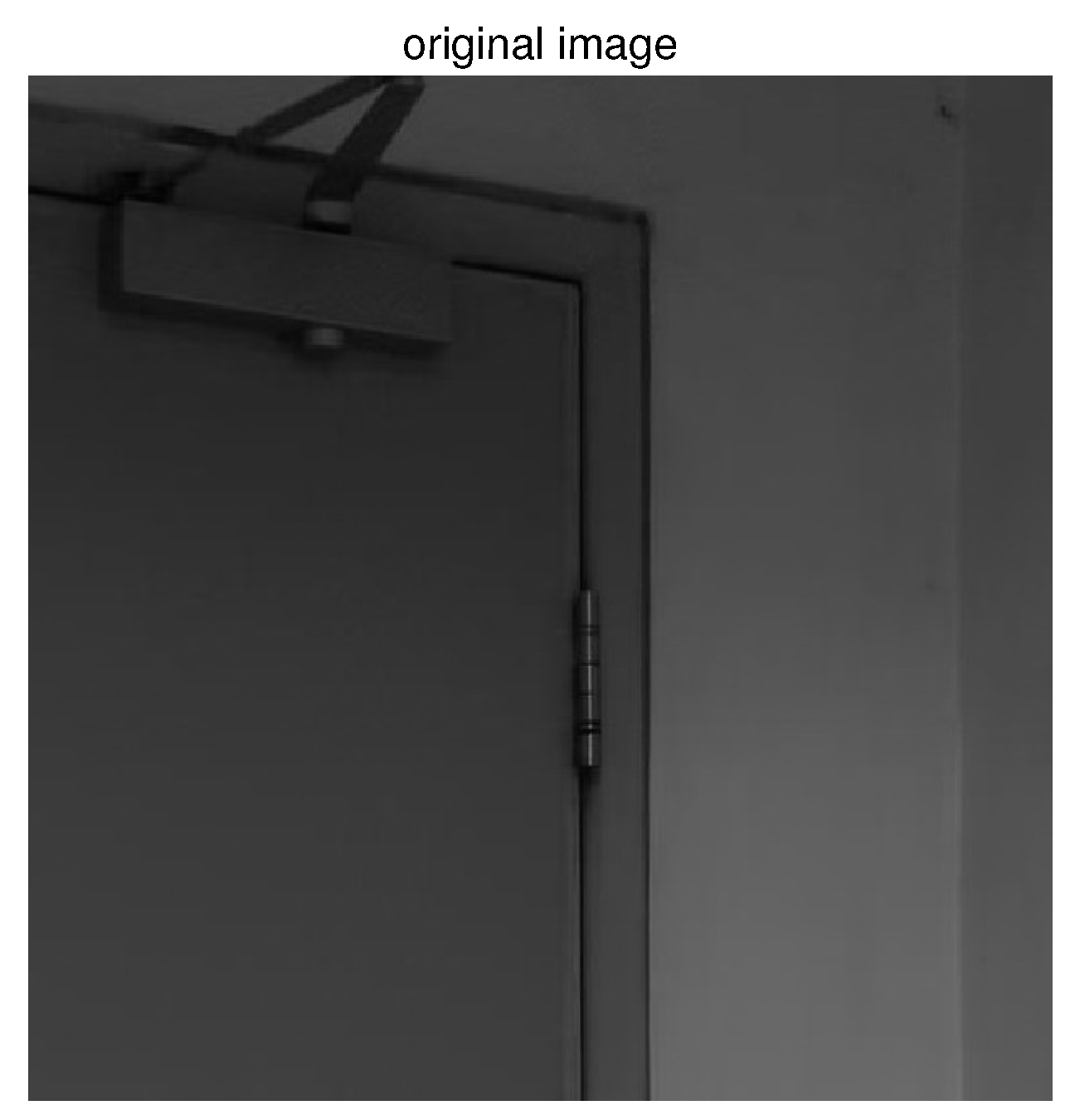
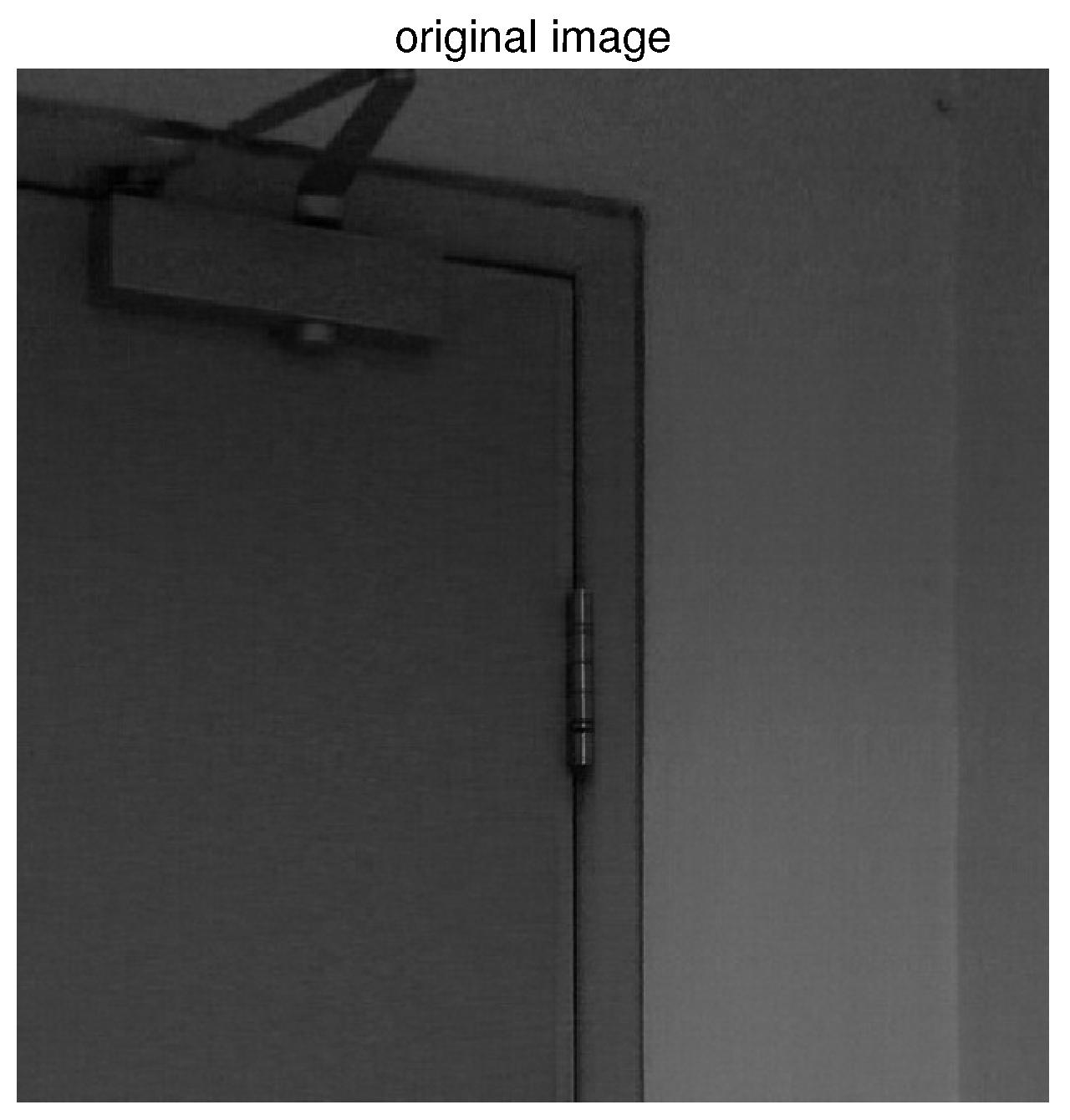
5.2. Experiment Results with Real Data
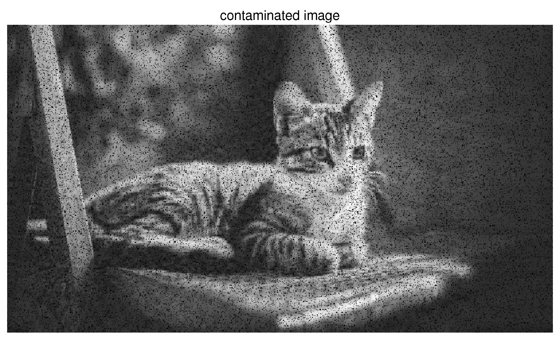
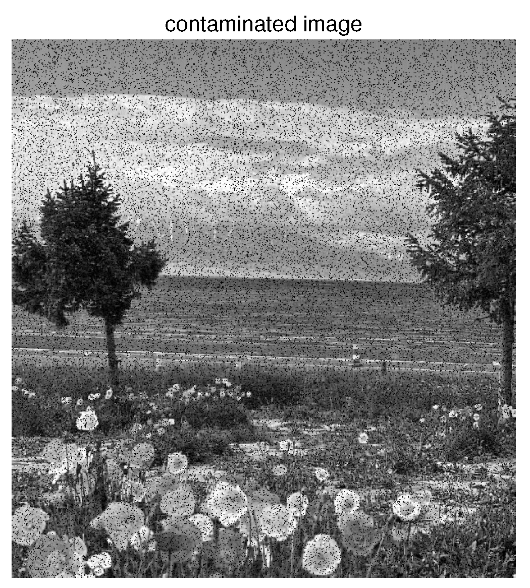
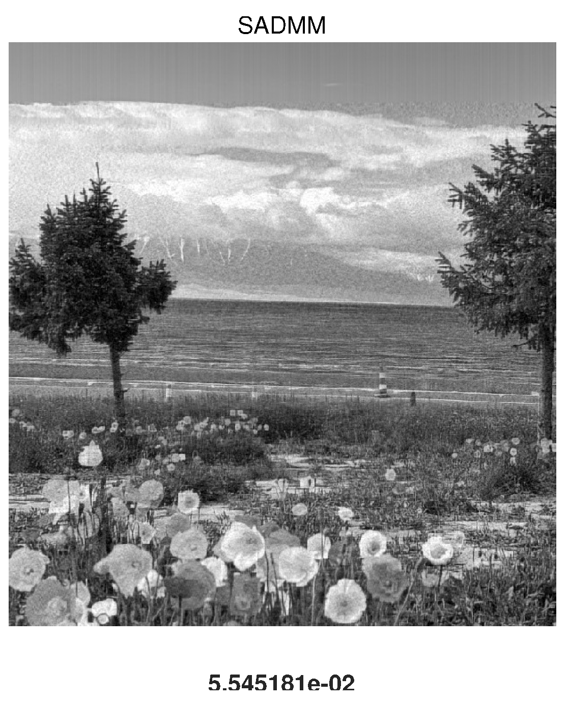
5.3. Experiment Results with Real Noisy Images
6. Discussion
7. Conclusions
Author Contributions
Funding
Institutional Review Board Statement
Informed Consent Statement
Data Availability Statement
Conflicts of Interest
Abbreviations
| MDPI | Multidisciplinary Digital Publishing Institute |
| DOAJ | Directory of Open-Access Journals |
| TLA | Three-letter acronym |
| LD | Linear dichroism |
References
- Jain, V.; Seung, H. Natural Image Denoising with Convolutional Networks. Adv. Neural Inf. Process. Syst. 2008, 24, 769–776. [Google Scholar]
- Liu, D.; Li, D.; Song, H. Image Quality Assessment Using Regularity of Color Distribution. IEEE Access 2016, 4, 4478–4483. [Google Scholar] [CrossRef]
- Kim, J.; Lee, J.K.; Lee, K.M. Accurate image super-resolution using very deep convolutional networks. In Proceedings of the IEEE Conference on Computer Vision and Pattern Recognition, Las Vegas, NV, USA, 27–30 June 2016; pp. 1646–1654. [Google Scholar]
- Tian, C.; Xu, Y.; Fei, L.; Yan, K. Deep Learning for Image Denoising: A Survey. In Advances in Intelligent Systems and Computing, Proceedings of the ICGEC 2018, Changzhou, China, 14–17 December 2018; Springer: Singapore, 2019; Volume 834. [Google Scholar]
- Puttagunta, M.; Ravi, S. Medical image analysis based on deep learning approach. Multimed. Tools Appl. 2021, 80, 24365–24398. [Google Scholar] [CrossRef]
- Vo, H.H.P.; Nguyen, T.M.; Yoo, M. Weighted Robust Tensor Principal Component Analysis for the Recovery of Complex Corrupted Data in a 5G-Enabled Internet of Things. Appl. Sci. 2024, 14, 4239. [Google Scholar] [CrossRef]
- Zhang, H.; Huang, D.; Wang, K. Denoising of Wrapped Phase in Digital Speckle Shearography Based on Convolutional Neural Network. Appl. Sci. 2024, 14, 4135. [Google Scholar] [CrossRef]
- Yi, J.; Jiang, H.; Wang, X. A Comprehensive Review on Sparse Representation and Compressed Perception in Optical Image Reconstruction. Arch. Comput. Methods Eng. 2024, 31, 3197–3209. [Google Scholar] [CrossRef]
- Yuan, Q.; Zhang, Q.; Li, J.; Shen, H.; Zhang, L. Hyperspectral image denoising employing a spatial–spectral deep residual convolutional neural network. IEEE Trans. Geosci. Remote Sens. 2019, 57, 1205–1218. [Google Scholar] [CrossRef]
- Bodrito, T.; Zouaoui, A.; Chanussot, J.; Mairal, J. A trainable spectral–spatial sparse coding model for hyperspectral image restoration. Proc. Adv. Neural Inf. Process. Syst. 2021, 34, 5430–5442. [Google Scholar]
- Bampis, E.; Escoffier, B.; Schewior, K.; Teiller, A. Online Multistage Subset Maximization Problems. Algorithmica 2021, 83, 2374–2399. [Google Scholar] [CrossRef]
- Eom, M.; Han, S.; Park, P. Statistically unbiased prediction enables accurate denoising of voltage imaging data. Nat. Methods 2023, 20, 1581–1592. [Google Scholar] [CrossRef]
- Buades, A.; Coll, B.; Morel, J.-M. A non-local algorithm for image denoising. In Proceedings of the 2005 IEEE Computer Society Conference on Computer Vision and Pattern Recognition, San Diego, CA, USA, 20–26 June 2005; Volume 2, pp. 60–65. [Google Scholar]
- Zhang, K.; Zuo, W.; Chen, Y.; Meng, D.; Zhang, L. Beyond a Gaussian Denoiser: Residual Learning of Deep CNN for Image Denoising. IEEE Trans. Image Process. 2017, 26, 3142–3155. [Google Scholar] [CrossRef] [PubMed]
- Candes, E.J.; Li, X.; Ma, Y.; Wright, J. Robust Principal Component Analysis? J. ACM 2011, 58, 37. [Google Scholar] [CrossRef]
- Muksimova, S.; Umirzakova, S.; Mardieva, S.; Cho, Y.I. Enhancing Medical Image Denoising with Innovative Teacher–Student Model-Based Approaches for Precision Diagnostics. Sensors 2023, 23, 9502. [Google Scholar] [CrossRef] [PubMed]
- Chen, Y.; Jalali, A.; Sanghavi, S.; Caramanis, C. Low-Rank Matrix Recovery From Errors and Erasures. IEEE Trans. Inf. Theory 2013, 59, 4324–4337. [Google Scholar] [CrossRef]
- Muksimova, S.; Mardieva, S.; Cho, Y.I. Deep Encoder–Decoder Network-Based Wildfire Segmentation Using Drone Images in Real-Time. Remote Sens. 2022, 14, 6302. [Google Scholar] [CrossRef]
- Li, X.; Zhu, Z.; Man-Cho So, A.; Vidal, R. Nonconvex Robust Low-Rank Matrix Recovery. SIAM J. Optim. 2020, 30, 660–686. [Google Scholar] [CrossRef]
- Huan, X.; Caramanis, C.; Sanghavi, S. Robust PCA via outlier pursuit. IEEE Trans. Inf. Theory 2012, 58, 3047–3064. [Google Scholar]
- Recht, B. A simpler approach to matrix completion. J. Mach. Learn. Res. 2011, 12, 3413–3430. [Google Scholar]
- Koko, J. Parallel Uzawa method for large-scale minimization of partially separable functions. J. Optim. Theory Appl. 2013, 158, 172–187. [Google Scholar] [CrossRef]
- Liu, Y.; Jiao, L.C.; Shang, F.; Yin, F.; Liu, F. An efficient matrix bi-factorization alternative optimization method for low-rank matrix recovery and completion. Neural Netw. 2013, 48, 8–18. [Google Scholar] [CrossRef]
- Hu, Y.; Liu, X.; Jacob, M. A Generalized Structured Low-Rank Matrix Completion Algorithm for MR Image Recovery. IEEE Trans. Med. Imaging 2019, 38, 1841–1851. [Google Scholar] [CrossRef] [PubMed]
- Iordache, M.D.; Bioucas-Dias, J.M.; Plaza, A. Collaborative Sparse Regression for Hyperspectral Unmixing. IEEE Trans. Geosci. Remote Sens. 2014, 52, 341–354. [Google Scholar] [CrossRef]
- Zhang, S.G. Projection and self-adaptive projection methods for the Signorini problem with the BEM. Appl. Math. Comput. 2017, 74, 1262–1273. [Google Scholar] [CrossRef]
- Zhang, S.; Li, X. A self-adaptive projection method for contact problems with the BEM. Appl. Math. Model. 2018, 55, 145–159. [Google Scholar] [CrossRef]
- Huang, Z.; Li, S.; Hu, F. Hyperspectral image denoising with multiscale low-rank matrix recovery. In Proceedings of the 2017 IEEE International Geoscience and Remote Sensing Symposium (IGARSS), Fort Worth, TX, USA, 23–28 July 2017; pp. 5442–5445. [Google Scholar]
- Mason, E.; Yazici, B. Robustness of LRMR based Passive Radar Imaging to Phase Errors. In Proceedings of the EUSAR 2016: 11th European Conference on Synthetic Aperture Radar, Hamburg, Germany, 6–9 June 2016; pp. 1–4. [Google Scholar]
- Zhou, P.; Lu, C.; Feng, J.; Lin, Z.; Yan, S. Tensor Low-Rank Representation for Data Recovery and Clustering. IEEE Trans. Pattern Anal. Mach. Intell. 2021, 43, 1718–1732. [Google Scholar] [CrossRef]
- Shen, Q.; Liang, Y.; Yi, S.; Zhao, J. Fast Universal Low Rank Representation. IEEE Trans. Circuits Syst. Video Technol. 2022, 32, 1262–1272. [Google Scholar] [CrossRef]
- Chen, T.; Xiang, Q.; Zhao, D.; Sun, L. An Unsupervised Image Denoising Method Using a Nonconvex Low-Rank Model with TV Regularization. Appl. Sci. 2023, 13, 7184. [Google Scholar] [CrossRef]
- Wu, B.; Yu, J.; Ren, H.; Lou, Y.; Liu, N. Seismic Traffic Noise Attenuation Using lp -Norm Robust PCA. IEEE Geosci. Remote Sens. Lett. 2020, 17, 1998–2001. [Google Scholar] [CrossRef]
- Xu, J.; Li, H.; Liang, Z.; Zhang, D.; Zhang, L. Real-world Noisy Image Denoising: A New Benchmark. arXiv 2018, arXiv:1804.02603. [Google Scholar] [CrossRef]


| Iteration | 5 | 10 | 25 | 100 |
|---|---|---|---|---|
| ADMM | 0.1962 | 0.1189 | 0.1115 | 0.1115 |
| S-ADMM | 0.9442 | 0.8575 | 0.5248 | 0.0542 |
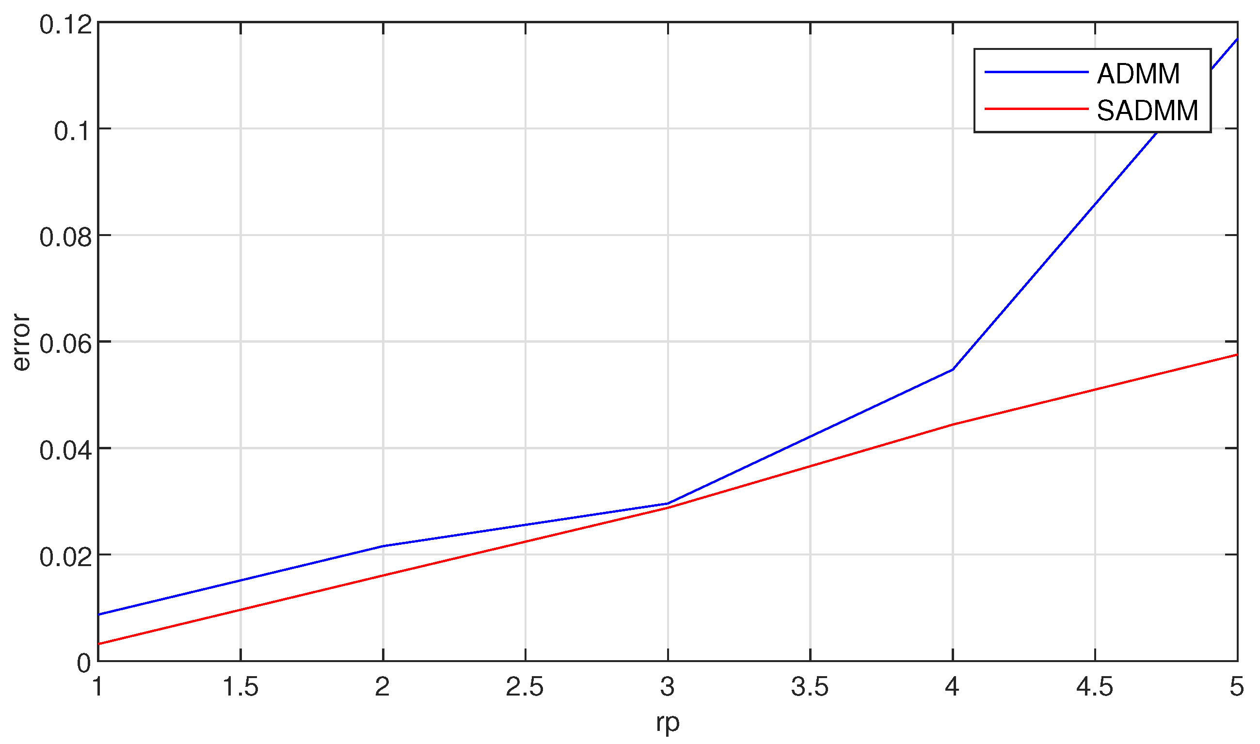
| 0.1 | 0.15 | 0.2 | 0.25 | 0.3 | |
|---|---|---|---|---|---|
| ADMM | 0.0079 | 0.0183 | 0.0313 | 0.0562 | 0.1115 |
| S-ADMM | 0.0027 | 0.0129 | 0.0308 | 0.0435 | 0.0542 |
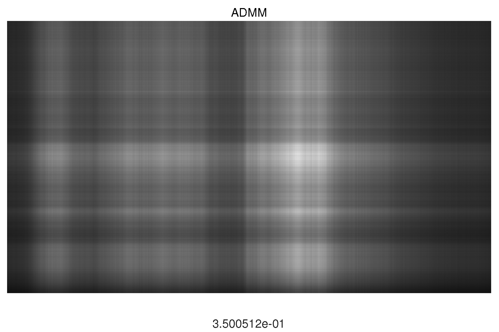
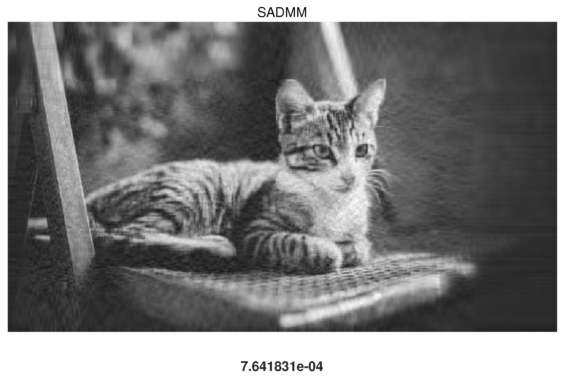
| Algorithm | SVT | ADMM | S-ADMM |
|---|---|---|---|
| MSE | 0.2503 | 0.3501 | |
| SSIM | 0.84977 | 0.74089 | 0.99395 |
| Algorithm | SVT | ADMM | S-ADMM |
|---|---|---|---|
| MSE | 0.2737 | 0.3214 | 0.0555 |
| SSIM | 0.62676 | 0.5018 | 0.96393 |
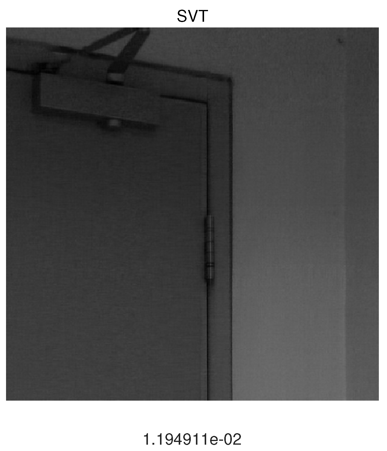
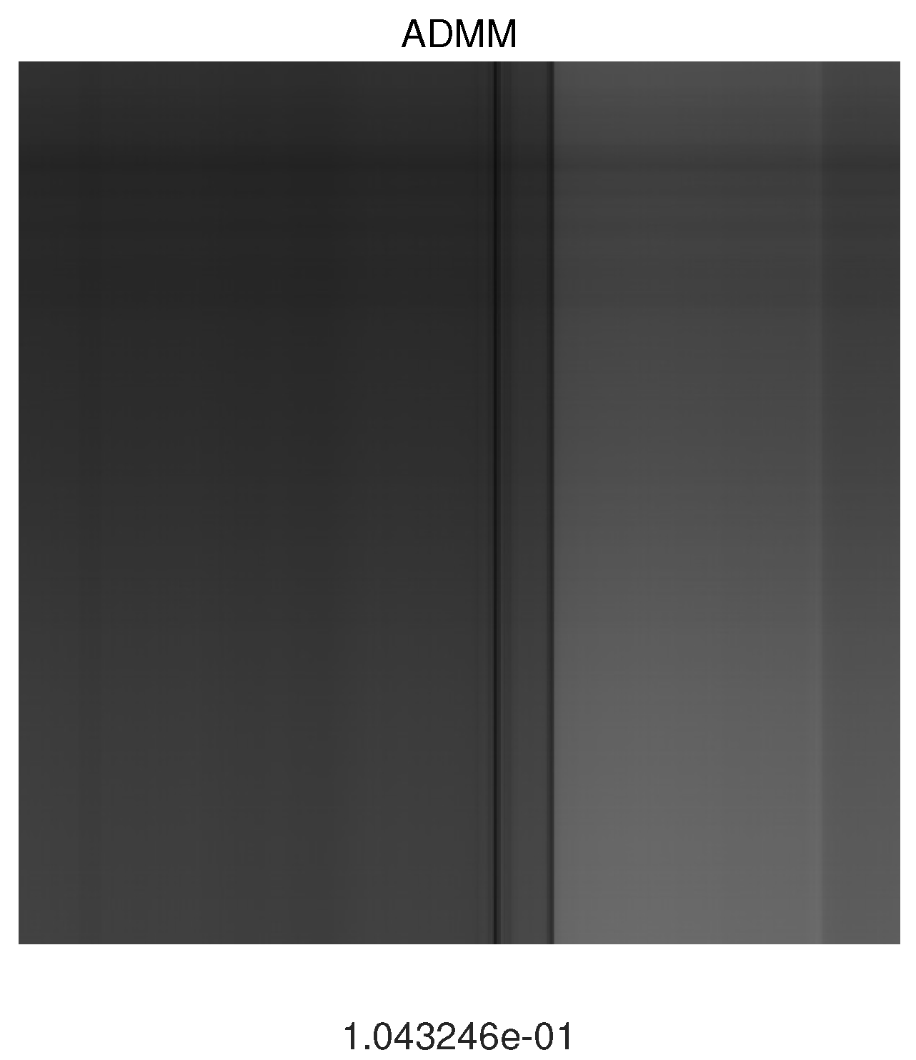
| Algorithm | SVT | ADMM | S-ADMM |
|---|---|---|---|
| MSE | 0.0119 | 0.1043 | 0.0093 |
| SSIM | 0.80704 | 0.96089 | 0.96561 |
Disclaimer/Publisher’s Note: The statements, opinions and data contained in all publications are solely those of the individual author(s) and contributor(s) and not of MDPI and/or the editor(s). MDPI and/or the editor(s) disclaim responsibility for any injury to people or property resulting from any ideas, methods, instructions or products referred to in the content. |
© 2024 by the authors. Licensee MDPI, Basel, Switzerland. This article is an open access article distributed under the terms and conditions of the Creative Commons Attribution (CC BY) license (https://creativecommons.org/licenses/by/4.0/).
Share and Cite
Xie, M.; Guo, H. Self-Adaptive Alternating Direction Method of Multipliers for Image Denoising. Appl. Sci. 2024, 14, 10427. https://doi.org/10.3390/app142210427
Xie M, Guo H. Self-Adaptive Alternating Direction Method of Multipliers for Image Denoising. Applied Sciences. 2024; 14(22):10427. https://doi.org/10.3390/app142210427
Chicago/Turabian StyleXie, Mingjie, and Haibing Guo. 2024. "Self-Adaptive Alternating Direction Method of Multipliers for Image Denoising" Applied Sciences 14, no. 22: 10427. https://doi.org/10.3390/app142210427
APA StyleXie, M., & Guo, H. (2024). Self-Adaptive Alternating Direction Method of Multipliers for Image Denoising. Applied Sciences, 14(22), 10427. https://doi.org/10.3390/app142210427