Advanced Distribution System Optimization: Utilizing Flexible Power Buses and Network Reconfiguration

Featured Application

Radial electrical power network optimizations through reconfigurations including generation and demand flexibility.

Abstract

The increasing integration of distributed generation (DG) and the rise of microgrids have reshaped the operation of distribution systems, introducing both challenges and opportunities for optimization. This study presents a methodology that combines network reconfiguration with the integration of buses with flexible power in order to improve the efficiency and cost-effectiveness of distribution networks. Flexible buses, which aggregate multiple microgrids or controllable distributed resources, function as control points that can dynamically adjust active and reactive power within predefined limits. This capability allows for more precise management of power flows, enabling the system to respond to fluctuations in generation and demand. The proposed optimization framework aims to minimize the total operational costs, including power losses and the use of flexible power, while adhering to system constraints. The methodology is evaluated through case studies on two distribution systems: the Kumamoto and IEEE-33 systems. The results indicate a 43.9% reduction in power losses for the Kumamoto system and a 66.6% reduction for the IEEE-33 system, along with notable cost savings in both cases. These outcomes demonstrate the potential benefits of incorporating flexible power buses in modern radial distribution networks, showing their role in adapting to various operational scenarios and supporting the integration of distributed generation and microgrids.

1. Introduction

The integration of distributed generation (DG) and the emergence of microgrids (µgrids) are reshaping the conventional operation of distribution systems. These technologies introduce new levels of flexibility and control, enabling more effective management of power flows [1,2]. As the penetration of renewable energy sources grows, along with advancements in energy storage and demand-side management, the traditional centralized approach to power distribution is evolving into a more decentralized and dynamic model [3,4].

Microgrids, typically comprising local DG units, energy storage, and controllable loads, can operate autonomously or in coordination with the main grid [5]. When connected to the larger distribution network, the aggregation of multiple microgrids at specific buses allows system operators to dynamically adjust power flows, enhancing both local optimization and overall network efficiency and stability [6,7,8].

Historically, power adjustment within distribution systems has been primarily used for contingency management, reacting to unexpected events to maintain stability [9,10]. However, with the increasing complexity and variability of modern power systems, there is a growing need for proactive strategies that leverage the flexibility of microgrids and distributed resources to optimize network performance under normal operating conditions [11,12]. This shift from reactive to proactive management requires new methodologies capable of dynamically reconfiguring the network and optimizing power flows to minimize operational costs, reduce losses, and maintain voltage stability.

In this context, this work introduces the concept of flexible power buses. These buses, representing aggregated microgrids or flexible resources, can dynamically adjust active and reactive power within predefined ranges. By integrating flexible power buses into the distribution network and applying network reconfiguration, the system can more effectively respond to varying demand and generation conditions, ultimately enhancing overall performance and resilience.

State of Art

In the scientific literature, there are numerous studies that combine distribution network reconfiguration, DG integration, optimization of DG placement and sizing, and the implementation of optimal power flow (OPF). However, the approach presented in this work introduces a subtle but significant variation from the existing literature.

In [13], Helmi et al. develop an algorithm based on Harris Hawks Optimization (HHO) to address the problem of distribution network reconfiguration, including µgrids. The objective is to minimize energy losses and improve voltage profiles by determining the optimal network topology. The approach includes a multi-stage optimization process that combines HHO with pre-processing and post-processing phases, which improve the initial generation of configurations and refine the solutions obtained. Lei et al., in their work titled “Radiality Constraints for Resilient Reconfiguration of Distribution Systems: Formulation and Application to Microgrid Formation” [14], as the title suggests, emphasize the importance of radiality constraints in systems that include flexible µgrids, explaining how they can contribute to system robustness by allowing dynamic network reconfiguration. Other authors have also studied µgrids/reconfigurations as a way to improve the system [15,16], including radial distribution systems [17,18]. The reconfigurations in the recent work published and described above [14] are based on graph theory, which has also been the foundation of the algorithm presented in this work. Additionally, Yaprakdal et al., in [19], highlight the innovation of reconfigurable microgrids (RMGs) in short-term optimization, combining network reconfiguration and optimal DG dispatch to minimize energy losses. They use a hybrid optimization approach based on particle swarm optimization (PSO), which enhances system efficiency and reliability, validated in an IEEE-33 system.

On the other hand, µgrids are increasingly recognized for their role in enhancing the flexibility of energy systems, enabling the integration of renewable energy sources, DG, and energy storage systems. Ramadan and Helmi [20] use the Manta Ray Foraging Optimization (MRFO) algorithm to improve fault tolerance and rapid recovery in smart grids through network reconfiguration, also achieving significant energy loss reduction and improvement in the voltage profile given different network scenarios. Recently, Gautam et al., in [21], propose a deep reinforcement learning approach for optimal distribution network reconfiguration, aimed at minimizing critical load loss during certain events (contingencies), achieving quick and effective reconfiguration even with changes in system states. Shi et al., in [22], develop a supply interruption management strategy that combines network reconfiguration with optimal distributed energy resource (DER) scheduling, enabling a high percentage of load to be maintained in service following network faults, highlighting the efficiency of the method compared to traditional µgrid formation approaches.

As the reconfigurations and DG management are investigated, the optimal placement of DG within an electrical system or µgrids is also studied. In [23], Badran et al. develop an optimization strategy that simultaneously determines the optimal reconfiguration of the distribution network and the DG power injection, with objectives such as minimizing energy loss, improving the voltage profile, and maximizing DG penetration. Using metaheuristic algorithms (Evolutionary Programming, PSO, Firefly, and GSA), they demonstrate that network reconfiguration alone is not sufficient to achieve maximum network performance. In this work, the authors highlight the crucial importance of optimal DG placement, although in their case study, they assume that this placement is optimal based on previous studies, specifically in [24], focusing therefore on optimizing DG injection.

Studies in this field are advancing by introducing and combining different optimization algorithms and merging various concepts into the problem to be optimized (functions, constraints, objectives, etc.). In the work [25] recently published by Raza et al., an ant colony optimization (ACOA)-based method is introduced, which optimizes both network reconfiguration and the placement and size of different types of DG, improving system stability and significantly reducing active power losses and voltage drops at the buses, all while maintaining the radial structure of the system and improving its reliability.

Regarding the approach followed in this work, it is essential to highlight the concept of optimal power flow, known as OPF. This method is a key tool in the operation and planning of electrical systems, as it aims to find the optimal point of control variables that minimize an objective function, generally associated with generation costs, while satisfying all system constraints [26,27]. The primary objective of OPF is to determine the optimal dispatch of generating units, adjust the voltage levels, and define power flow through the network, all in a way that minimizes the costs associated with operation, such as fuel costs, and maximizes system efficiency. Additionally, in some approaches/algorithms, OPF may also consider minimizing active and reactive power losses, as well as optimizing the voltage profile in the network. However, it is important to note that traditional OPF methods usually assume a fixed network topology, which means that the network structure does not change during the optimization process. This assumption limits the applicability of OPF in systems that may require dynamic reconfiguration, either for operational reasons or in response to contingencies. In this context, research has emerged that integrates network topology reconfiguration with OPF, allowing greater system flexibility and adaptability to changes [28,29,30].

This work presents a comprehensive approach that combines network reconfiguration with the implementation of flexible power buses to address challenges arising from increased distributed generation (DG) penetration, microgrid integration, gradual and growing electricity demand, and the stochastic variability of renewable production. The main contributions of this work are as follows:

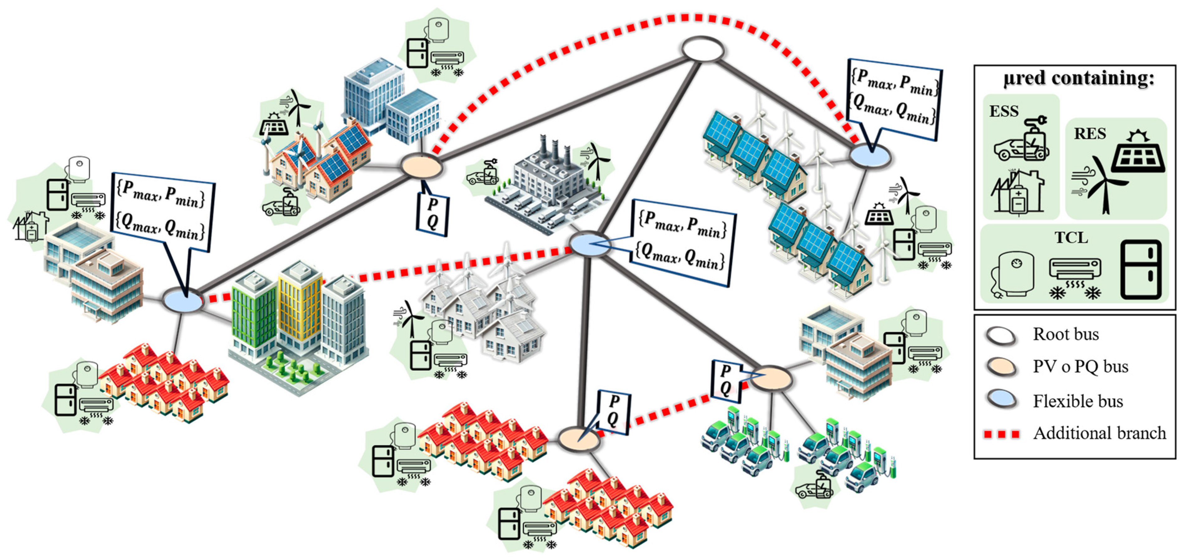
• Flexible Power Buses: The concept of flexible power buses is introduced, where each bus can dynamically adjust its active and reactive power within a predefined range in order to satisfy distribution system requirements. This flexibility allows for better adaptation to varying demand and generation conditions, enhancing overall system performance. This concept will be discussed in the next section.
• Integration of Flexible Power Buses with System Reconfiguration: The proposed algorithm systematically explores all possible radial configurations derived from the base system, incorporating flexible buses. By assessing each potential configuration, the method ensures that the global optimal solution is identified. This approach enables the distribution system to dynamically adapt to changes in demand and DG, providing a more robust and efficient operational topology.
• Optimization Framework: A comprehensive formulation of the optimization problem is presented, defining key decision variables, objective functions, and constraints. The framework integrates load flow analysis, allowing for precise adjustments to active (P) and reactive (Q) power flows. The optimization aims to minimize both operational costs and power losses, leading to a more efficient and cost-effective distribution network.

The remainder of this paper is organized as follows: Section 2 provides an overview of the approach. Section 3 covers key technical components, including power flow analysis (Section 3.1), the reconfiguration algorithm (Section 3.2), and the optimization problem formulation (Section 3.3). Section 4 presents two case studies: the Kumamoto and IEEE-33 system, demonstrating the effectiveness of the proposed approach. Finally, Section 5 concludes the work with a discussion of the results and potential future research directions.

2. Overview of the Approach

The proposed methodology for optimizing distribution systems through network reconfiguration and the use of flexible buses aims to address operational optimization. Unlike traditional approaches that focus solely on the optimal placement and sizing of DG, this method also integrates demand/generation flexibility. This allows for the precise adjustment of active and reactive power variables (P and Q) at designated flexible buses.

2.1. Concept of Flexible Buses

The concept of a flexible power bus refers to a specific point within the electrical network designed to centralize control over a set of small, geographically distributed electrical installations. These installations, often organized as microgrids, collectively contribute to the network’s generation and demand capabilities. When multiple microgrids are interconnected and linked to the main grid, they create a centralized node known as the Point of Common Coupling (PCC). This PCC acts as a flexible power bus, where aggregated power adjustments can be managed for both active and reactive power. It provides the system operator with a single, centralized location to control the power flows from all connected installations downstream, thus facilitating power management capabilities [31,32].

This flexibility is possible through the integration of various distributed energy resources (DERs) and/or controllable loads within the network. For example, thermostatic loads, which are prevalent in many electrical installations, can be adjusted without violating user comfort limits, allowing for controlled variations in power consumption [33]. Similarly, photovoltaic panels and small wind turbines can be regulated by modifying their operating points, such as adjusting maximum power point tracking (MPPT) settings [34,35]. Energy storage systems, whether stationary batteries or those integrated into electric vehicles, provide additional flexibility by allowing the injection or absorption of power based on network needs [36]. Moreover, flexible buses can take advantage of deferrable and controllable loads [37,38], like dishwashers and washing machines, that can shift their operation to periods of lower demand or higher renewable generation. In this context, DG is represented within the flexible bus concept.

When modeled, these buses differ from traditional PQ or PV buses, where power is typically fixed to a certain value. Instead, in this optimization problem, flexible buses are modeled as PQ buses, but the P/Q value can vary within predefined limits, represented as $\{P_{max},P_{min}\}$ and $\{Q_{max},Q_{min}\}$. This margin is given by the available generation and demand resources downstream of the PCC.

In a practical implementation, when optimizing the system, the operator identifies potential flexible buses by collecting detailed information on the PCCs of microgrids, distributed installations, and controllable resources across the network. This process includes assessing each bus’s capability to adjust power in terms of both generation and demand, as well as determining the specific power adjustment margins available.

In Figure 1, the flexible power buses are highlighted in blue.

2.2. Procedure

The flowchart in Figure 2 summarizes the complete methodology. Starting from the base radial configuration, the approach identifies buses with demand and generation flexibility, along with alternative branches for potential reconfiguration. The reconfiguration algorithm (highlighted in blue) systematically generates all possible radial configurations by incorporating these additional branches. Each configuration is then evaluated by the optimization framework (in grey), which adjusts P and Q at the flexible buses, taking into account constraints such as power limits and voltage levels across the system. The objective function aims to minimize both power loss costs and the costs associated with using flexible power. Ultimately, the configuration with the lowest objective function value is selected as the most efficient topology.

The flowchart highlights two key components: the reconfiguration algorithm and the optimization framework, each distinguished by colour for clarity. The reconfiguration algorithm focuses on generating potential configurations by exploring different combinations of branches and flexible buses, ensuring all configurations maintain radiality. Meanwhile, the optimization framework evaluates these configurations by determining the optimal P and Q settings at the flexible buses. Within this framework, load flow analysis plays a critical role, involving network modeling and the calculation of various electrical parameters, such as the voltage levels, power flows, and compliance with operational constraints. This comprehensive approach ensures that the system can dynamically adapt to changes in demand and generation, leading to a more efficient and resilient distribution network.

3. Methodology

In this section, the proposed approach for optimizing distribution systems through network reconfiguration and the utilization of flexible buses is presented. As discussed, the methodology comprises three main components: power flow analysis, reconfiguration algorithm, and optimization framework. Each of these components contributes to achieving a system configuration that minimizes operational costs while maintaining network stability and efficiency.

3.1. Power Flow Analysis

Power distribution systems predominantly operate in a radial configuration, favored for its simplicity, cost-effectiveness, and ease of fault isolation [39,40]. This structure, characterized by a single path from the source to each load, ensures efficient design and straightforward operation. Although some systems may incorporate limited meshing to meet specific operational needs, the radial layout remains the preferred choice due to its lower installation and maintenance costs, as well as the ease of integrating distributed energy resources (DERs). Radial configurations simplify fault detection and isolation, minimizing downtime and facilitating network management, which is crucial for maintaining stability. Additionally, the radial topology aligns well with typical urban and suburban network layouts, where loads are distributed across wide areas, making direct connections to substations more efficient. These advantages underscore why the radial structure is fundamental to power flow analysis and why it serves as the basis for the proposed optimization approach.

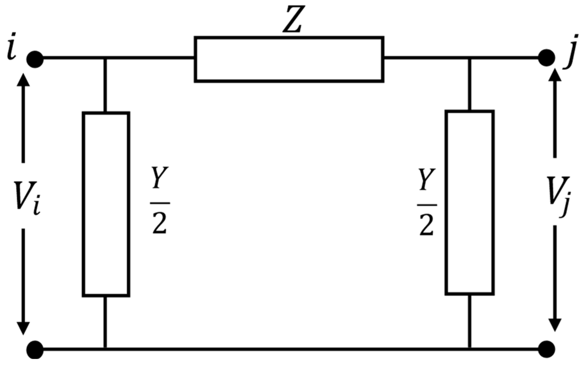
3.1.1. Network Modeling

The main components of a distribution network are buses, transmission lines, loads, and generators [41]. Buses serve as connection points where these elements converge, and these buses can be classified into three types:

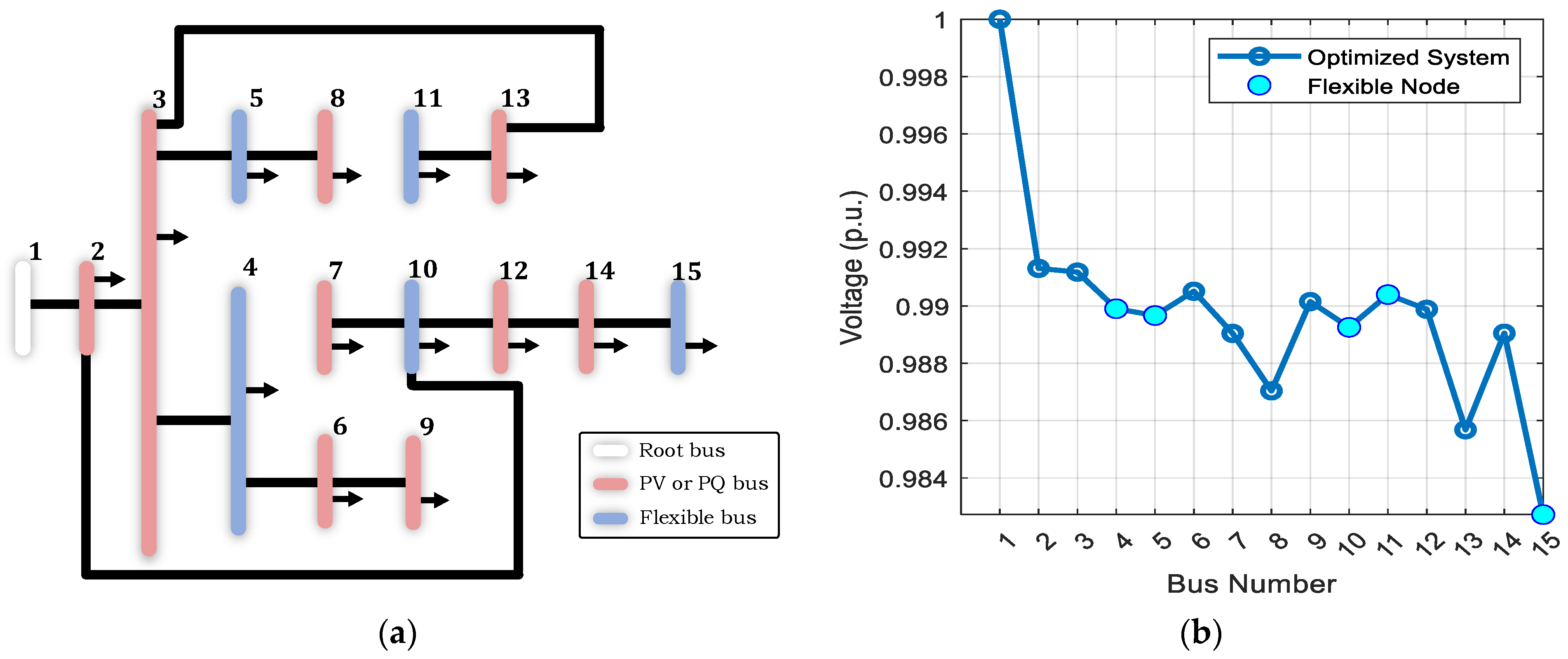
• Root Bus: acts as a reference point with a predefined voltage magnitude and phase angle.
• PQ Bus: defines specified levels of active (P) and reactive (Q) power.
• PV Bus: specifies active power (P) and voltage magnitude (V).

Transmission lines are represented using a $\pi$-equivalent circuit model, which includes both series impedance and shunt admittance. The series impedance $Z=R+jX$ accounts for resistance ($R$) and reactance ($X$), while the shunt admittance $Y$ reflects the line charging effect. This circuit model is illustrated in Figure 3.

The power generated by the generators at specific buses is expressed as follows:

$$S_{gen,i}=P_{gen,i}+j{Q}_{gen,i}$$

(1)

Meanwhile, loads are modeled as constant power requirements at each bus:

$$S_{load,i}=P_{load,i}+j{Q}_{load,i}$$

(2)

Calculating power flow in distribution systems relies on applying Kirchhoff’s laws to determine bus voltages and line currents under steady-state conditions. Due to the distinct features of these systems, such as their high $R/X$ ratios and predominantly radial topology, traditional power flow methods may not be as efficient. Instead, more tailored approaches, like the forward/backward sweep algorithm [42], are used to leverage the network’s radial layout, streamlining the process and improving convergence rates.

To further enhance the efficiency of these calculations, the use of BIBC (Bus Injection to Branch Current) and BCBV (Branch Current to Bus Voltage) matrices has been introduced. These methods help simplify the mapping of currents and voltages across the network [43].

3.1.2. BIBC, BCBV, and DLF Matrices

The BIBC matrix establishes the link between the current injected at various nodes and the currents flowing through the network branches [43]. It essentially encodes the network’s connectivity, capturing how current inputs at the nodes translate into currents along the lines. Mathematically, this can be expressed as follows:

$$I_b=BIBC·I_{inj}$$

(3)

where $I_{inj}$ is the vector of node current injections, and $I_b$ is the resulting vector of branch currents.

In a radial configuration, the BIBC matrix has a lower triangular form, reflecting the hierarchical, tree-like structure of the network. Each element ${BIBC}_{ij}$ is set to 1 if node$j$ is located upstream of node $i$, and 0 otherwise.

Complementary to the BIBC, the BCBV matrix describes how branch currents influence voltage drops across the network nodes [43]. This matrix inherently integrates the impedance characteristics of the network’s branches, converting the branch current vector ($I_b$) into a vector of node voltage drops ($∆V$). The transformation can be represented by the following:

$$∆V=BCBV·I_b$$

(4)

The construction of the BCBV matrix depends directly on the impedance values of each branch. For a network composed of $n$nodes, the matrix will have a dimensionality of (n − 1) × (n − 1) corresponding to the n − 1 branches typically present in a radial layout.

By combining these two matrices, a more comprehensive tool known as the Distribution Load Flow (DLF) matrix can be derived. This composite matrix provides a streamlined way to calculate voltage drops across nodes directly from current injections, eliminating the need for intermediate calculations involving branch currents. The DLF matrix is defined by the following:

$$DLF=BCBV·BIBC$$

(5)

Thus, the node voltage drop vector can be directly obtained as follows:

$$∆V=DLF·I_{inj}$$

(6)

A notable feature of the BIBC, BCBV, and consequently the DLF matrix is their stability: they remain constant as long as the network topology does not change. This constancy is particularly advantageous for repeated load flow analysis, as it allows for efficient calculations without needing to recompute these matrices unless there are structural changes in the system.

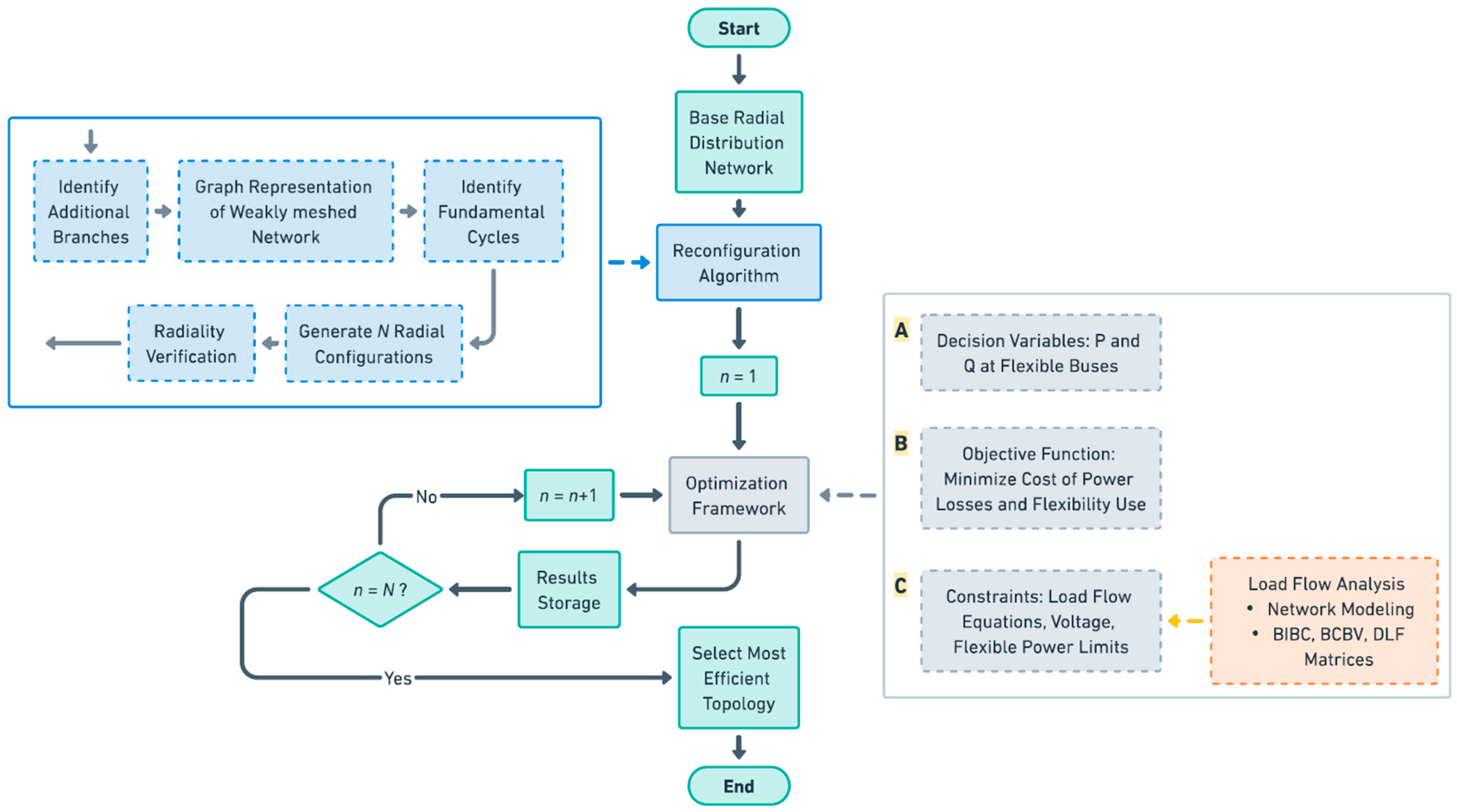
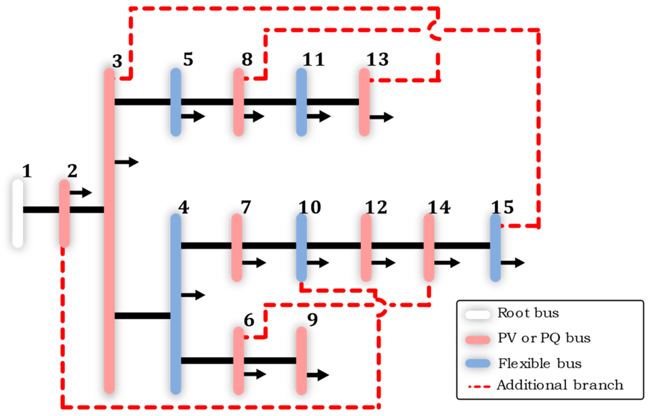
3.2. Reconfiguration Algorithm

Reconfiguration in radial distribution networks is a process that modifies the network topology by opening or closing line switches in response to changes in demand and generation conditions. The main goal of reconfiguration is to improve the network’s efficiency and reliability while preserving its radial structure, which simplifies the operation and control of the power system [44]. This process is essential for balancing loads, minimizing power losses, and responding to faults or maintenance needs without disrupting the overall power supply.

Graph theory provides a robust mathematical framework to model and analyze electrical distribution networks. In this context, the network is represented as a graph, where nodes (or vertices) correspond to buses, and edges (or branches) represent the power lines connecting these buses. It provides a robust mathematical framework to model and analyze electrical distribution networks, aiding in their reconfiguration. In [45], the authors demonstrated the use of graph theory to efficiently handle network reconfiguration in DC zonal electric distribution systems. The authors utilized graph-based numerical methods to solve optimization problems, ensuring power balance while minimizing switching operations. Similarly, Ref. [46] integrated graph theory with particle swarm optimization to minimize power loss and enhance the voltage profiles in distribution systems, highlighting the method’s feasibility for network reconfiguration. One of the main challenges in reconfiguring electrical distribution networks is ensuring that the network maintains a radial (tree-like) structure. Graph theory aids in this process by enabling the identification of redundant paths (cycles) and facilitating the calculation of feasible network topologies. Using techniques such as cycle identification, minimum spanning trees, and adjacency matrices, graph theory helps to simplify and streamline the reconfiguration process, making it more efficient. To develop the reconfiguration method presented in this work, various MATLAB functions were utilized to facilitate each of the necessary tasks. These functions provided robust tools for the analysis and manipulation of electrical networks, simplifying and optimizing each stage of the reconfiguration algorithm. The process is divided into five key steps:

• Graph Representation: The network is represented as an undirected graph $G(V,E)$ where $V$ is the set of buses and $E$ is the set of branches. The adjacency matrix $A$ describes the network connectivity, providing a foundation for further analysis. The MATLAB function graph is used to construct this representation [47].
• Identification of Fundamental Cycles: Fundamental cycles, which represent redundant paths that break the radial structure, are identified using MATLAB’s cyclebasis function [48]. These cycles are the primary targets for branch elimination to ensure the network maintains a radial configuration.
• Generation of Radial Configurations: All possible radial configurations are generated by selectively eliminating branches from the identified fundamental cycles. The MATLAB nchoosek function [49] is employed to calculate all possible combinations of branch elimination, ensuring that only unique configurations are considered.
• Radiality Verification: Each generated configuration is checked for radiality using the cyclebasis function again. Any configuration that still contains cycles is discarded, ensuring that only valid radial topologies are retained.
• Bus Reorganization and Branch Orientation: Before performing load flow analysis, the buses are reorganized according to their hierarchical structure. A minimum spanning tree is generated using MATLAB’s minspantree function [50], ensuring correct orientation and connectivity from the root bus towards the leaves.

This structured approach reduces computational complexity by focusing on branch elimination within detected cycles, enabling the efficient generation and evaluation of radial configurations.

3.3. Optimization Problem Formulation

Once the algorithm has identified all possible branch combinations to form radial systems, the optimization process begins on a system-by-system basis. The optimization process involves the following elements:

• Decision Variable

The decision variables for this optimization problem are the active (P) and reactive (Q) power at the flexible buses in the distribution system. These variables allow the system to dynamically respond to demand and generation needs. For each flexible bus i, the decision variables are represented as follows:

$$\begin{array}{c}{P}_{nudoflexiblei}\\ Q_{nudoflexiblei}\end{array}$$

(7)

B.

Objective Function

The objective of the optimization problem is to minimize the total costs associated with the operation of the distribution system. These costs include both active power losses in the network and the costs related to the use of flexible power at buses that allow variability in active and reactive power injection. Therefore, the goal is to determine, for each radial configuration generated by the algorithm, the optimal values of P and Q at the flexible buses, minimizing the economic impact of both active power losses and the use of flexibility at these buses.

$$\mathrm{M}\mathrm{i}\mathrm{n}\mathrm{i}\mathrm{m}\mathrm{i}\mathrm{z}\mathrm{e}{C}_{totals}=C_{PP}·P_{TS}+C_{PF}·S_{FTU}$$

(8)

where

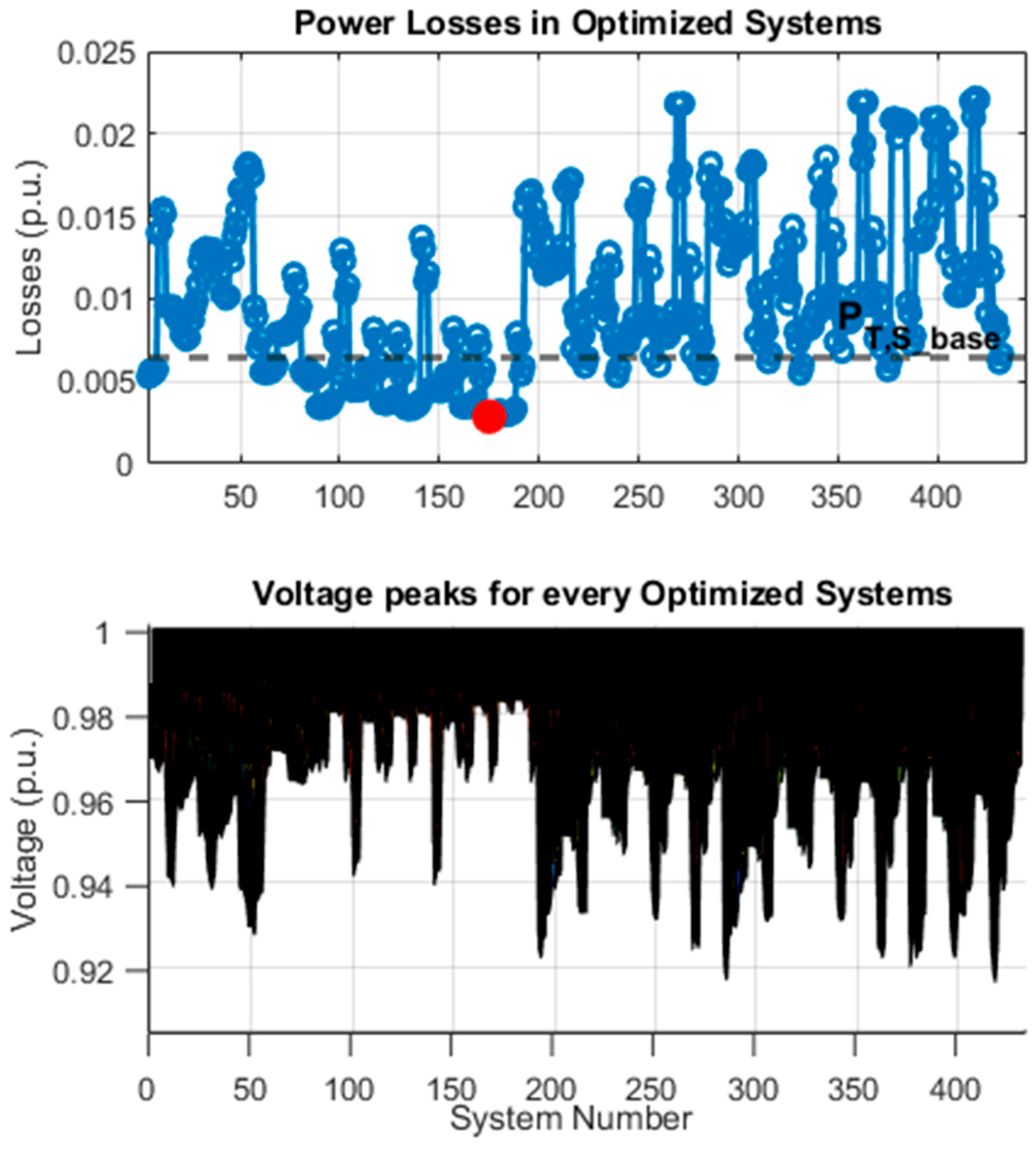
• $P_{TS}$ represents the total active power losses of the system.
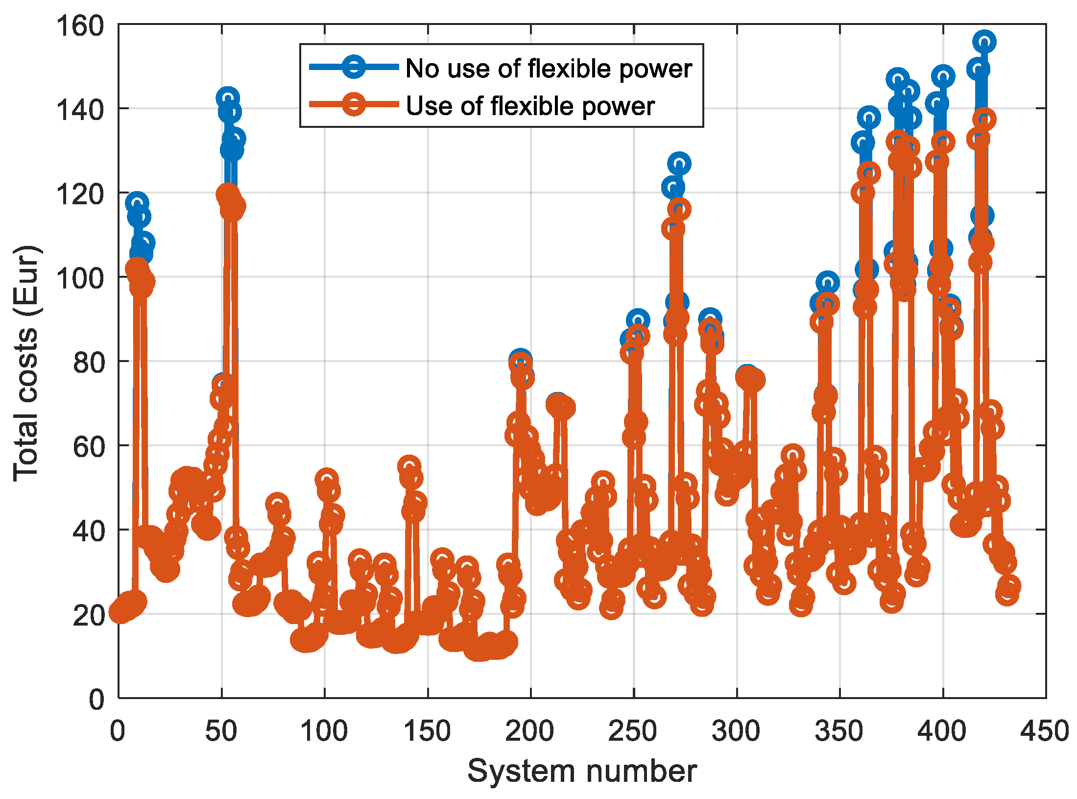
• $S_{FTU}$ represents the amount of flexible power used at the flexible buses.
• $C_{PP}$ is the cost associated with active power losses.
• $C_{PF}$ is the cost associated with the use of flexible power.

The flexible power utilized, $S_{FTU}$, is defined as follows:

$$S_{FTU}=\sqrt{{\left(P_{FTU}\right)}^2+{\left(Q_{FTU}\right)}^2}$$

(9)

The values of $P_{FTU}$ and $Q_{FTU}$ are calculated as follows:

$$\begin{gathered} P_{FTU}=\left|P_{baseinical}-P_{nudoflexiblei}\right| \\ {Q}_{FTU}=\left|Q_{baseinical}-Q_{nudoflexiblei}\right| \end{gathered}$$

(10)

where $P_{baseinical}$ and $Q_{baseinical}$ are the active and reactive power of the base system, respectively, and $P_{nudoflexiblei}$ and $Q_{nudoflexiblei}$ are the decision variables of the optimization problem as previously defined. If the values of P and Q have not changed, then the associated costs for that term will be zero.

C.

Constraints

The optimization problem must satisfy several operational constraints to ensure that the proposed solution is feasible and secure:

• Load flow equations:

These equations ensure the balance of active and reactive power at each bus of the system. They are represented as follows:

$$\begin{gathered} P_i=V_i\sum _{n=1}^N\left[V_n(G_{in}cos{\delta }_{in}+B_{in}sen{\delta }_{in})\right] \\ {Q}_i=V_i\sum _{n=1}^N\left[V_n(G_{in}sen{\delta }_{in}-B_{in}cos{\delta }_{in})\right] \end{gathered}$$

(11)

where $P_i$ and $Q_i$ are the active and reactive power at buses $i$, $V_i$ and $V_n$ are the voltage magnitudes at buses $i$ and $n$, $G_{in}$ and $B_{in}$ are the conductance and susceptance between buses $i$ and $n$, and ${\delta }_{in}={\delta }_i-{\delta }_n$ is the phase angle difference between buses $i$ and $n$.

2.

Power at flexible buses:

The range of power that the decision variable can take is limited as follows:

$$\begin{gathered} P_{min}\le P_{nudoflexiblei}\le P_{max} \\ {Q}_{min}\le Q_{nudoflexiblei}\le Q_{max} \end{gathered}$$

(12)

3.

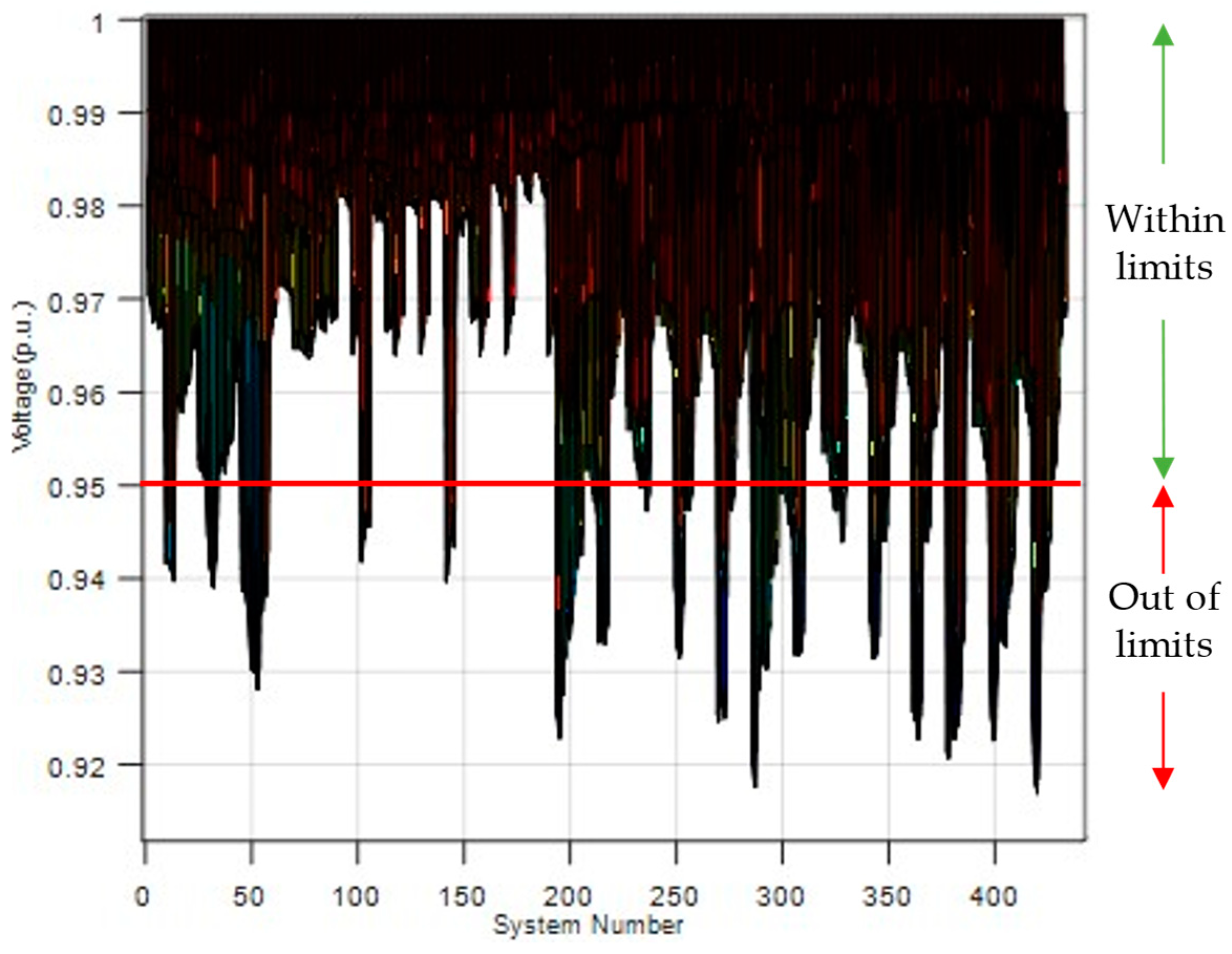
Voltage:

The voltage at all buses must remain within appropriate limits to ensure the normal and safe operation of the network:

$$V_{min}\le V_{nudoi}\le V_{max}$$

(13)

4.

Radiality:

In most optimization problems applied to distribution systems involving reconfiguration, radiality constraints are typically incorporated to ensure that the network maintains its radial structure during the optimization process. However, in the proposed methodology, this constraint is not necessary. This is because a previous algorithm generates all possible radial configurations of the system. As a result, the optimizer operates exclusively on configurations that are already radial, eliminating the need to impose additional radiality constraints during the optimization process.

D.

Optimizer

The optimization problem is solved using the MATLAB function fmincon [51], which is suitable for finding the minimum of an objective function subject to constraints. fmincon uses the “interior-point” algorithm by default, which converts a constrained problem into a series of unconstrained problems by adding a barrier to the objective function. This barrier prevents the solutions from approaching too close to the constraint boundaries, keeping them within the feasible region. As the algorithm progresses, the influence of the barrier is reduced, allowing the solution to approach the optimum within the permitted limits.

The interior-point algorithm follows a path known as the “central path”, guiding the solution toward the optimum while remaining within the feasible region. During this process, the algorithm ensures that the Karush–Kuhn–Tucker (KKT) conditions [52], which are fundamental to guaranteeing optimality in constrained optimization problems, are met. These conditions include primal feasibility, dual feasibility, stationarity, and complementary slackness.

This methodological approach is implemented systematically, evaluating all possible radial configurations and adjusting the flexible buses’ variables to find the most efficient configuration with minimized operational costs.

4. Use Cases

To evaluate the effectiveness of the proposed optimization algorithm applied to distribution systems through reconfiguration and flexible buses, these use cases analyze how the optimization of a distribution system can lead to significant improvements. The selected distribution systems are the Kumamoto and IEEE-33 systems.

4.1. Kumamoto System

The Kumamoto system consists of 15 buses, including 1 root bus and 14 PQ buses. The network operates at a base voltage of 6.6 kV and a base power of 10 MVA. Detailed data on the buses and branches comprising this system are provided in [53]. For this study, additional branches were considered to enable the reconfiguration of the network, as shown in Figure 4. A list of these additional branches is provided in

Table 1. Parameters of additional branches in the Kumamoto system.

From	To	R (p.u.)	X (p.u.)
6	14	0.0607	0.00754
15	8	0.00732	0.01694
3	13	0.0307	0.032346
2	10	0.0012	0.022

.

In this approach, flexible buses are introduced, allowing adjustments in both active and reactive power, as depicted in blue in Figure 4. Unlike traditional PV buses, where active power is known and reactive power is adjusted to maintain a specific voltage level, flexible buses do not have a fixed voltage setpoint. Instead, the optimization process ensures that the voltages at all system buses, including the flexible buses, remain within predefined limits, specifically between 0.95 and 1.05 p.u. Instead, the active and reactive power at these buses can vary within a specified range. The optimization process determines the optimal values of P and Q at these flexible buses, ensuring that the voltages at all system buses remain within predefined limits. This adjustability makes flexible buses more suitable for system optimization under dynamic conditions.

The system operates with nominal PQ values of the Kumamoto network, i.e., base values ($P_{baseinical}$and $Q_{baseinical}$). The optimization process begins by identifying which buses have flexibility, specifically in this proposed scenario, buses 4, 5, 10, 11, and 15. In addition to identifying which buses can have flexibility in active and reactive power values, the algorithm specifies the range for these values. These details for the case study are shown in

Table 2. Range of active and reactive power values for the flexible buses, Kumamoto system.

Bus Number	Interval over Initial Value (%)	$\mathbf{Active}\mathbf{Power}\left(\mathit{P}\right)$ (p.u.)			$\mathbf{Reactive}\mathbf{Power}\left(\mathit{Q}\right)$ (p.u.)
		Minimum Value	Initial Value (Base)	Maximum Value	Minimum Value	Initial Value (Base)	Maximum Value
4	50	0.0479	0.0958	0.1437	0.0049	0.0098	0.0147
5	50	0.0066	0.0132	0.0198	0.0007	0.0014	0.0021
10	50	0.01615	0.0323	0.04845	0.00165	0.0033	0.00495
11	50	0.00805	0.0161	0.02415	0.0008	0.0016	0.0024
15	50	0.1085	0.2170	0.3255	0.011	0.0220	0.033

. These buses were chosen randomly to act as flexible buses, simulating potential locations of flexibility. In a real system, the selection of flexible buses would depend on a detailed assessment of available distributed resources and their power adjustment capabilities.

To maintain a systematic approach, and given that this is a simulated scenario, a fixed percentage has been applied to the initial value of the distribution system to determine the maximum and minimum power values for all buses, which is set at 50%. However, it should be noted that these values could be different or randomly assigned for each bus, as the optimizer can work with any specified power range.

The cost associated with power losses is 0.4 EUR/kW, and the cost associated with flexible power is 0.04 EUR/kVA.

The algorithm code is executed in Matlab on a PC with an AMD Ryzen 5 2500U processor, Radeon Vega Mobile Gfx at 2.00 GHz, and 16.0 GB of RAM.

Once the algorithm has been applied to the Kumamoto system in Figure 4 and has optimized all feasible radial systems, the optimal system is presented, and the overall results are evaluated. The runtime was 52.8784 s.

A total of 432 feasible systems were found, and all of them were optimized. The system labeled as number 175 had the lowest total costs and is therefore considered the optimal configuration. In Figure 5a,b, the topology and voltage profile of this optimal system are shown, respectively. Compared to the initial system, lines 4–7 and 8–11 are disconnected, while lines 2–10 and 3–13 are connected.

The initial system exhibits 0.006484695 p.u. (64.85 kW) of power loss, with a cost of EUR 25.9387, while the optimal system shows 0.0028515 p.u. (28.5 kW) with a cost of EUR 11.406210. For the initial system, the total cost is equal to the cost of losses since no flexible power is being used. In contrast, in the optimized system, there is a cost of EUR 0.000013, indicating minimal use of flexible power. In the optimal system, power losses are reduced by 43.9% compared to the initial system, resulting in significant cost savings.

The reason for the minimal use of flexible power in this system is due to the low profitability it would represent for the total calculation of losses, i.e., using flexible power would not have a sufficiently profitable impact to justify its use.

In Figure 6a, the total power losses for each optimized system are shown, compared to the initial system (indicated by a dashed black line). It can be observed that a significant number of optimized configurations exhibit lower losses compared to the initial system, demonstrating the effectiveness of the optimization algorithm in improving system efficiency in several cases. However, 309 systems out of a total of 432 show higher losses after optimization. In the graph, system number 175, highlighted in red, stands out as the optimal system, achieving the lowest losses. On the other hand, Figure 6b represents the total costs associated with each optimized system. Comparing both graphs, it is noted that the relationship between power losses and costs is not directly proportional. This is because, in many cases, the algorithm has made considerable use of flexible power to reduce costs, which explains why, although some systems present higher losses, they are compensated with a reduction in total costs.

In Figure 7, the surface of voltage profiles for each bus in the different optimized systems is illustrated. This three-dimensional graph allows visualization of how voltages vary depending on the system configuration and the buses considered. It is evident that not all configurations meet the voltage constraints, as voltage peaks outside the permitted range (0.95 ≤ V ≤ 1.05) can be observed.

To delve deeper into this analysis, Figure 8 presents a closer view of the voltage peaks in the different optimized systems. Here, systems that do not meet the voltage constraints are highlighted, clearly showing how the voltage profiles of some systems fall below the lower limit of 0.95 p.u., disqualifying them as viable configurations. This analysis is crucial as it allows for the automatic filtering and discarding of configurations that do not meet the voltage constraints. Although these constraints have been established in the optimizer, it may happen that, among the various reconfigured systems, no combination of active and reactive power values at the flexible buses results in a system with voltage values within the range due to the nature of the topology (buses’ organization). A total of 89 reconfigured systems out of the 432 total do not meet the imposed voltage limits.

Figure 9 shows the correlation between voltages and power losses, providing a combined view that allows comparing the “performance” of each system from both perspectives. It is observed that systems with better voltage profiles, i.e., those with smaller voltage drops throughout their profile, tend to present lower power losses. This suggests that good voltage control is not only necessary to maintain good voltage levels in the system but is also associated with higher efficiency in terms of power losses. In contrast, systems that show greater voltage drops tend to have higher losses.

Figure 10 displays the total costs of optimized systems both with (in orange) and without (in blue) the use of flexible power. The objective of this figure is to verify the optimization algorithm’s functionality and its ability to reduce total costs through the intelligent use of flexible power. Comparing both sets of data, it is observed that the use of flexible power (represented in orange) is predominant in those systems where its application is profitable. This is clearly evident starting from approximately EUR 80. At this point, systems that use flexible power achieve a significant reduction in total costs compared to those that do not use it (represented in blue). This confirms that the optimizer makes appropriate decisions, applying flexible power in configurations where its economic impact is significant, allowing for a cost reduction when it is most advantageous to do so. Thus, it can be verified that the algorithm not only identifies optimal configurations in terms of power losses but also knows when it is profitable to use flexible power to minimize total costs.

In the simulated scenario, there were reconfigurations that did not require the use of flexible power for optimization, as incorporating it would have increased the overall operational costs of the distribution system. However, it is important to note that this may not always be the case. Under different conditions or scenarios, it is possible that all reconfigured systems could exhibit higher operational costs compared to the base case, necessitating the use of flexible power to minimize costs. In such situations, the optimization algorithm becomes crucial, as it intelligently determines when the application of flexible power is economically advantageous, ensuring that the total system costs are reduced whenever possible. This adaptability highlights the importance of the proposed approach, demonstrating its capability not only to optimize reconfiguration but also to strategically utilize flexible power to achieve cost-effective solutions under various operational scenarios.

4.2. IEEE-33 System

The IEEE-33 system consists of 33 buses, including a root bus and 32 PQ buses, operating at a base voltage of 12.66 kV and a base power of 100 MVA. Detailed information on the buses and branches of the IEEE-33 system, as well as the additional branches used for reconfiguration, can be found in [54]. The additional branches considered are 8–14, 7–20, 11–21, and 24–28.

Flexible buses are also introduced, which allows adjustments in both active and reactive power. These flexible buses, represented as nodes 9, 5, 17, 21, 30, 26, and 25, follow the base power settings of the IEEE-33 system. The flexibility range for active and reactive power is determined based on a fixed percentage, similar to the approach used in the Kumamoto system. The interval of allowed variation for the active and reactive power values is shown in

Table 3. Range of active and reactive power values for the flexible buses, IEEE-33 system.

Bus Number	Interval over Initial Value (%)	$\mathbf{Active}\mathbf{Power}\left(\mathit{P}\right)$ (p.u.)			$\mathbf{Reactive}\mathbf{Power}\left(\mathit{Q}\right)$ (p.u.)
		Minimum Value	Initial Value (Base)	Maximum Value	Minimum Value	Initial Value (Base)	Maximum Value
9	35	0.00039	0.0006	0.00081	0.00013	0.0002	0.00027
5	50	0.0003	0.0006	0.0009	0.00015	0.0003	0.00045
17	15	0.00051	0.0006	0.00069	0.00017	0.0002	0.00023
21	20	0.00072	0.0009	0.00108	0.00032	0.0004	0.00048
25	32	0.00286	0.0042	0.00554	0.00136	0.002	0.00264

, reflecting the flexibility needed for optimization.

The cost parameters are set at 0.4 EUR/kW for power losses and 0.04 EUR/kVA for flexible power usage.

The execution resulted in the identification and optimization of 2241 feasible radial systems, with the optimal system identified as system number 1577, yielding significant cost reductions.

The runtime for this case was 369.13 s. The initial IEEE-33 system exhibited 0.0021 p.u. (210 kW) of power loss with a total cost of EUR 84.4. After optimization, the optimal configuration, identified as system number 1577, showed a power loss of 0.0014 p.u. (140 kW) with a total cost of EUR 55.48. This reflects a power loss reduction of 66.6% and a significant cost saving. The optimal configuration for the IEEE-33 system did not utilize flexible power, as the cost–benefit analysis determined that its application would not result in a profitable outcome, similar to the findings observed in the Kumamoto case. However, there are configurations where the use of flexible power contributed to a reduction in the total costs, as illustrated in Figure 11.

5. Conclusions

This study presents a methodology for optimizing distribution systems through network reconfiguration and the use of flexible buses. With the increasing penetration of distributed generation, the rise of microgrids, and advancements in power system controllability, the integration of flexible buses becomes essential. These buses represent the sum of several microgrids connected to a point in the system, providing a range of values for active and reactive power adjustments. This approach allows for the dynamic optimization of power flows, enhancing the network’s efficiency and adaptability under varying distributed generation and demand scenarios.

A notable feature of this algorithm is its ability to evaluate all possible radial configurations that can arise from the base system. Unlike conventional optimization techniques, which may only consider a subset of potential configurations, this methodology ensures that all feasible radial systems are evaluated, guaranteeing that the global optimal solution is identified.

The optimization problem is formulated with clear decision variables and objective functions, enabling the systematic adjustment of power variables at flexible buses. This minimizes the operational costs and power losses, while accommodating the flexibility introduced by new technologies and the integration of distributed energy resources.

The application of this methodology to the Kumamoto and IEEE-33 system case study shows a 43.9% and 66.6%, respectively, reduction in power losses compared to the initial configuration, with a corresponding decrease in operational costs. This demonstrates the potential of the proposed approach in improving distribution network performance and highlights the significance of flexible buses in modern power systems.

References

- Shi, W.; Xie, X.; Chu, C.-C.; Gadh, R. Distributed Optimal Energy Management in Microgrids. IEEE Trans. Smart Grid 2015, 6, 1137–1146. [Google Scholar] [CrossRef]
- Chang, W.-N.; Chang, C.-M.; Yen, S.-K. Improvements in Bidirectional Power-Flow Balancing and Electric Power Quality of a Microgrid with Unbalanced Distributed Generators and Loads by Using Shunt Compensators. Energies 2018, 11, 3305. [Google Scholar] [CrossRef]
- Mahmoud, M.S.; Saif Ur Rahman, M.; A.L.-Sunni, F.M. Review of Microgrid Architectures—A System of Systems Perspective. IET Renew. Power Gener. 2015, 9, 1064–1078. [Google Scholar] [CrossRef]
- Han, Y.; Zhang, K.; Li, H.; Coelho, E.A.A.; Guerrero, J.M. MAS-Based Distributed Coordinated Control and Optimization in Microgrid and Microgrid Clusters: A Comprehensive Overview. IEEE Trans. Power Electron. 2018, 33, 6488–6508. [Google Scholar] [CrossRef]
- Wang, J.; Li, K.-J.; Javid, Z.; Sun, Y. Distributed Optimal Coordinated Operation for Distribution System with the Integration of Residential Microgrids. Appl. Sci. 2019, 9, 2136. [Google Scholar] [CrossRef]
- Hu, P.; Chen, H.; Chen, C.; Liu, X. Optimal Integration of Microgrid for Distribution Network. In Proceedings of the 2015 IEEE PES Asia-Pacific Power and Energy Engineering Conference (APPEEC), Brisbane, Australia, 15–18 November 2015; pp. 1–5. [Google Scholar]
- Liu, W.; Zhuang, P.; Liang, H.; Peng, J.; Huang, Z. Distributed Economic Dispatch in Microgrids Based on Cooperative Reinforcement Learning. IEEE Trans. Neural Netw. Learn. Syst. 2018, 29, 2192–2203. [Google Scholar] [CrossRef]
- Tong, X.; Hu, C.; Zheng, C.; Rui, T.; Wang, B.; Shen, W. Energy Market Management for Distribution Network with a Multi-Microgrid System: A Dynamic Game Approach. Appl. Sci. 2019, 9, 5436. [Google Scholar] [CrossRef]
- Babaei, S.; Jiang, R.; Zhao, C. Distributionally Robust Distribution Network Configuration Under Random Contingency. IEEE Trans. Power Syst. 2020, 35, 3332–3341. [Google Scholar] [CrossRef]
- Clavijo-Camacho, J.; Ruiz-Rodriguez, F.J. Improving the Reliability of an Electric Power System by Biomass-Fueled Gas Engine. Energies 2022, 15, 8451. [Google Scholar] [CrossRef]
- Wang, C.; Hou, Y.; Qiu, F.; Lei, S.; Liu, K. Resilience Enhancement with Sequentially Proactive Operation Strategies. IEEE Trans. Power Syst. 2017, 32, 2847–2857. [Google Scholar] [CrossRef]
- Park, S.; Shin, H. A Proactive Microgrid Management Strategy for Resilience Enhancement Based on Nested Chance Constrained Problems. Appl. Sci. 2022, 12, 12649. [Google Scholar] [CrossRef]
- Helmi, A.M.; Carli, R.; Dotoli, M.; Ramadan, H.S. Efficient and Sustainable Reconfiguration of Distribution Networks via Metaheuristic Optimization. IEEE Trans. Autom. Sci. Eng. 2022, 19, 82–98. [Google Scholar] [CrossRef]
- Lei, S.; Chen, C.; Song, Y.; Hou, Y. Radiality Constraints for Resilient Reconfiguration of Distribution Systems: Formulation and Application to Microgrid Formation. IEEE Trans. Smart Grid 2020, 11, 3944–3956. [Google Scholar] [CrossRef]
- Shariatzadeh, F.; Vellaithurai, C.B.; Biswas, S.S.; Zamora, R.; Srivastava, A.K. Real-Time Implementation of Intelligent Reconfiguration Algorithm for Microgrid. IEEE Trans. Sustain. Energy 2014, 5, 598–607. [Google Scholar] [CrossRef]
- Dall’Anese, E.; Giannakis, G.B. Risk-Constrained Microgrid Reconfiguration Using Group Sparsity. IEEE Trans. Sustain. Energy 2014, 5, 1415–1425. [Google Scholar] [CrossRef]
- Macedo, L.H.; Franco, J.F.; Mahdavi, M.; Romero, R. A Contribution to the Optimization of the Reconfiguration Problem in Radial Distribution Systems. J. Control Autom. Electr. Syst. 2018, 29, 756–768. [Google Scholar] [CrossRef]
- Kahouli, O.; Alsaif, H.; Bouteraa, Y.; Ben Ali, N.; Chaabene, M. Power System Reconfiguration in Distribution Network for Improving Reliability Using Genetic Algorithm and Particle Swarm Optimization. Appl. Sci. 2021, 11, 3092. [Google Scholar] [CrossRef]
- Yaprakdal, F.; Baysal, M.; Anvari-Moghaddam, A. Optimal Operational Scheduling of Reconfigurable Microgrids in Presence of Renewable Energy Sources. Energies 2019, 12, 1858. [Google Scholar] [CrossRef]
- Ramadan, H.S.; Helmi, A.M. Optimal Reconfiguration for Vulnerable Radial Smart Grids under Uncertain Operating Conditions. Comput. Electr. Eng. 2021, 93, 107310. [Google Scholar] [CrossRef]
- Gautam, M.; Abdelmalak, M.; MansourLakouraj, M.; Benidris, M.; Livani, H. Reconfiguration of Distribution Networks for Resilience Enhancement: A Deep Reinforcement Learning-Based Approach. In Proceedings of the 2022 IEEE Industry Applications Society Annual Meeting (IAS), Detroit, MI, USA, 9–14 October 2022; pp. 1–6. [Google Scholar]
- Shi, Q.; Li, F.; Olama, M.; Dong, J.; Xue, Y.; Starke, M.; Winstead, C.; Kuruganti, T. Network Reconfiguration and Distributed Energy Resource Scheduling for Improved Distribution System Resilience. Int. J. Electr. Power Energy Syst. 2021, 124, 106355. [Google Scholar] [CrossRef]
- Badran, O.; Mokhlis, H.; Mekhilef, S.; Dahalan, W. Multi-Objective Network Reconfiguration with Optimal DG Output Using Meta-Heuristic Search Algorithms. Arab. J. Sci. Eng. 2018, 43, 2673–2686. [Google Scholar] [CrossRef]
- Rao, R.S.; Ravindra, K.; Satish, K.; Narasimham, S.V.L. Power Loss Minimization in Distribution System Using Network Reconfiguration in the Presence of Distributed Generation. IEEE Trans. Power Syst. 2013, 28, 317–325. [Google Scholar] [CrossRef]
- Raza, A.; Zahid, M.; Chen, J.; Qaisar, S.M.; Ilahi, T.; Waqar, A.; Alzahrani, A. A Novel Integration Technique for Optimal Location & Sizing of DG Units with Reconfiguration in Radial Distribution Networks Considering Reliability. IEEE Access 2023, 11, 123610–123624. [Google Scholar] [CrossRef]
- Zimmerman, R.D.; Edmundo Murillo-Sanchez, C.; Thomas, R.J. MATPOWER: Steady-State Operations, Planning, and Analysis Tools for Power Systems Research and Education. IEEE Trans. Power Syst. 2011, 26, 12–19. [Google Scholar] [CrossRef]
- Alanazi, M.; Alanazi, A.; Abdelaziz, A.Y.; Siano, P. Power Flow Optimization by Integrating Novel Metaheuristic Algorithms and Adopting Renewables to Improve Power System Operation. Appl. Sci. 2023, 13, 527. [Google Scholar] [CrossRef]
- Wen, J.; Tan, Y.; Jiang, L.; Xu, Z. A Compound Objective Reconfiguration of Distribution Networks Using Hierarchical Encoded Particle Swarm Optimization. J. Cent. South Univ. 2018, 25, 600–615. [Google Scholar] [CrossRef]
- Hamour, H.; Kamel, S.; Abdel-mawgoud, H.; Korashy, A.; Jurado, F. Distribution Network Reconfiguration Using Grasshopper Optimization Algorithm for Power Loss Minimization. In Proceedings of the 2018 International Conference on Smart Energy Systems and Technologies (SEST), Seville, Spain, 10–12 September 2018; pp. 1–5. [Google Scholar]
- Merzoug, Y.; Abdelkrim, B.; Larbi, B. Distribution Network Reconfiguration for Loss Reduction Using PSO Method. Int. J. Electr. Comput. Eng. (IJECE) 2020, 10, 5009–5015. [Google Scholar] [CrossRef]
- Legry, M.; Dieulot, J.-Y.; Colas, F.; Saudemont, C.; Ducarme, O. Non-Linear Primary Control Mapping for Droop-Like Behavior of Microgrid Systems. IEEE Trans. Smart Grid 2020, 11, 4604–4613. [Google Scholar] [CrossRef]
- Legry, M.; Dieulot, J.-Y.; Colas, F.; Bakri, R. Model Predictive Control-Based Supervisor for Primary Support of Grid-Interactive Microgrids. Control Eng. Pract. 2023, 134, 105458. [Google Scholar] [CrossRef]
- Wang, Y.; Tang, Y.; Xu, Y.; Xu, Y. A Distributed Control Scheme of Thermostatically Controlled Loads for the Building-Microgrid Community. IEEE Trans. Sustain. Energy 2020, 11, 350–360. [Google Scholar] [CrossRef]
- Martin, A.D.; Cano, J.M.; Medina-Garcia, J.; Gomez-Galan, J.A.; Vazquez, J.R.; Martin, A.D.; Cano, J.M.; Medina-Garcia, J.; Gomez-Galan, J.A.; Vazquez, J.R. Centralized MPPT Controller System of PV Modules by a Wireless Sensor Network. IEEE Access 2020, 8, 71694–71707. [Google Scholar] [CrossRef]
- Torreglosa, J.P.; García, P.; Fernández, L.M.; Jurado, F. Energy Dispatching Based on Predictive Controller of an Off-Grid Wind Turbine/Photovoltaic/Hydrogen/Battery Hybrid System. Renew. Energy 2015, 74, 326–336. [Google Scholar] [CrossRef]
- Chen, L.; Wu, T.; Xu, X. Optimal Configuration of Different Energy Storage Batteries for Providing Auxiliary Service and Economic Revenue. Appl. Sci. 2018, 8, 2633. [Google Scholar] [CrossRef]
- Chen, Z.; Chen, Y.; He, R.; Liu, J.; Gao, M.; Zhang, L. Multi-Objective Residential Load Scheduling Approach for Demand Response in Smart Grid. Sust. Cities Soc. 2022, 76, 103530. [Google Scholar] [CrossRef]
- Li, Y.; Feng, B.; Wang, B.; Sun, S. Joint Planning of Distributed Generations and Energy Storage in Active Distribution Networks: A Bi-Level Programming Approach. Energy 2022, 245, 123226. [Google Scholar] [CrossRef]
- Chandramohan, S.; Kumudini Devi, R.P.; Venkatesh, D.B. Reliable Reconfiguration of Radial Systems—An Analysis. In Proceedings of the 2005 Annual IEEE India Conference—Indicon, Chennai, India, 11–13 December 2005; pp. 148–151. [Google Scholar]
- Li, Z.; Shahidehpour, M.; Alabdulwahab, A.; Al-Turki, Y. Valuation of Distributed Energy Resources in Active Distribution Networks. Electr. J. 2019, 32, 27–36. [Google Scholar] [CrossRef]
- Gomez-Exposito, A.; Conejo, A.J.; Canizares, C. Electric Energy Systems: Analysis and Operation; CRC Press: Boca Raton, FL, USA; London, UK; New York, NY, USA, 2020; ISBN 978-0-367-73427-5. [Google Scholar]
- Shirmohammadi, D.; Hong, H.W.; Semlyen, A.; Luo, G.X. A Compensation-Based Power Flow Method for Weakly Meshed Distribution and Transmission Networks. IEEE Trans. Power Syst. 1988, 3, 753–762. [Google Scholar] [CrossRef]
- Teng, J.-H. A Direct Approach for Distribution System Load Flow Solutions. IEEE Trans. Power Deliv. 2003, 18, 882–887. [Google Scholar] [CrossRef]
- Kumar, R.M.; Thanushkodi, K. Network Reconfiguration and Restoration in Distribution Systems through Oppostion Based Differential Evolution Algorithm and PGSA. In Proceedings of the 2013 International Conference on Current Trends in Engineering and Technology (ICCTET), Coimbatore, India, 3 July 2013; pp. 284–290. [Google Scholar]
- Certuche-Alzate, J.P.; Velez-Reyes, M. A Reconfiguration Algorithm for a DC Zonal Electric Distribution System Based on Graph Theory Methods. In Proceedings of the 2009 IEEE Electric Ship Technologies Symposium, Baltimore, MD, USA, 20–22 April 2009; pp. 235–241. [Google Scholar]
- Assadian, M.; Farsangi, M.M.; Nezamabadi-pour, H. GCPSO in Cooperation with Graph Theory to Distribution Network Reconfiguration for Energy Saving. Energy Convers. Manag. 2010, 51, 418–427. [Google Scholar] [CrossRef]
- Graph—Graph with Undirected Edges—MATLAB—MathWorks España. Available online: https://es.mathworks.com/help/matlab/ref/graph.html (accessed on 25 October 2024).
- Cyclebasis—Fundamental Cycle Basis of Graph—MATLAB—MathWorks España. Available online: https://es.mathworks.com/help/matlab/ref/graph.cyclebasis.html (accessed on 25 October 2024).
- Nchoosek—Coeficiente Binominal o Todas Las Combinaciones—MATLAB—MathWorks España. Available online: https://es.mathworks.com/help/matlab/ref/nchoosek.html (accessed on 25 October 2024).
- Minspantree—Minimum Spanning Tree of Graph—MATLAB—MathWorks España. Available online: https://es.mathworks.com/help/matlab/ref/graph.minspantree.html (accessed on 25 October 2024).
- Fmincon—Encontrar El Mínimo de Una Función Multivariable No Lineal Restringida—MATLAB—MathWorks España. Available online: https://es.mathworks.com/help/optim/ug/fmincon.html (accessed on 25 October 2024).
- Absil, P.-A.; Tits, A.L. Newton-KKT Interior-Point Methods for Indefinite Quadratic Programming. Comput. Optim. Appl. 2007, 36, 5–41. [Google Scholar] [CrossRef]
- Roy, N.K.; Pota, H.R.; Anwar, A. A New Approach for Wind and Solar Type DG Placement in Power Distribution Networks to Enhance Systems Stability. In Proceedings of the 2012 IEEE International Power Engineering and Optimization Conference, Melaka, Malaysia, 6–7 June 2012; IEEE: Piscataway, NJ, USA; pp. 296–301. [Google Scholar]
- Ruiz-Rodriguez, F.J.; Kamel, S.; Hassan, M.H.; Duenas, J.A. Optimal Reconfiguration of Distribution Systems Considering Reliability: Introducing Long-Term Memory Component AEO Algorithm. Expert Syst. Appl. 2024, 249, 123467. [Google Scholar] [CrossRef]