Spatiotemporal Analysis of Light Purse Seine Fishing Vessel Operations in the Arabian High Seas Based on Automatic Identification System Data

Abstract

Understanding the dynamic spatial distribution and characteristics of fishing activities is crucial for fisheries management and sustainable development. In recent years, small pelagic fish and cephalopods in the Arabian Sea have become new targets for light purse seine fishing; however, there is a lack of publicly available reports. This study uses automatic identification system (AIS) data from January to May and October to December of 2021 to 2022 in the region between 58°–70° E and 10°–22° N to extract spatial distribution information through three methods. The results show that with a spatial resolution of 0.25° × 0.25°, the spatial similarity index between the fishing ground information extracted in 2022 and catch data was consistently above 0.60, reaching 0.76 in March 2021 and 0.79 in November 2022, while the spatial similarity index in March 2022 exceeded 0.71. The spatial distribution of fishing effort and kernel density was similar to that of the fishing grounds, and the fishing intensity information exhibited the highest spatiotemporal similarity with commercial catch data, making it more suitable as a substitute for fishery data. Therefore, effective international cooperation and efficient joint management mechanisms for fishing vessels are needed to enhance the regulatory oversight of fishing vessels in this region. Integrating AIS data with other technological methods is crucial for more effective monitoring and management of fishing vessels. The findings presented in this paper provide both quantitative and qualitative scientific support for resource conservation and sustainable development in the region.

1. Introduction

With the increase in the number of global fishing vessels and advancements in fishing technology, global fishing efforts have surged significantly. This rapid increase presents formidable challenges to global fisheries management and sustainable development, exacerbated by both limited regulatory power and the absence of refined fishery information [1,2]. Understanding the distribution range of fishing vessel activities in fishing grounds, along with fishing intensity and other relevant information, is crucial for comprehending fishing pressure in these areas. Additionally, it indirectly reveals spatial changes in fishery resources and aids in monitoring illegal fishing activities [3,4], providing indispensable scientific support for the protection of marine fishery resources. The automatic identification system (AIS) provides trajectory information for fishing vessels, enabling the precise mapping of the spatial distribution of fishing intensity [5,6,7]. The AIS is instrumental in assessing fishing pressure within fishing grounds [8] and analyzing the operating behavior of fishing vessels [9,10]. As such, the AIS has emerged as a pivotal tool for fisheries resource management, fishing vessel regulation, and marine ecology protection.

High-resolution fishing activity information can indirectly reflect the spatial distribution of fishery resources and fishing grounds to a considerable extent [11]. AIS data have been effectively utilized for extracting spatial information on fishing grounds. In essence, the aggregation range of vessel operation positions and fishing intensity is often defined as fishing grounds [12]. Various spatial methods have been employed for this purpose; for instance, Sun et al. [13] utilized hotspot analysis to extract spatial information on fishing grounds in the North Pacific Ocean, while Guyader et al. [14] applied the kernel density method to derive information on bottom trawl fishing grounds in the western part of the Bay of Brest. These studies confirm that AIS data can be mined for spatiotemporal, high-precision fishing ground information. Chen et al. [15] integrated two methods, kernel density estimation (KDE) and hotspot analysis (HSA), to extract the hotspot areas of fishing activities in the Bohai Sea of China by mapping high-precision fishing grounds. This study emphasized that the combination of KDE and HSA was more effective than the individual use of these methods. The existing methodologies examine the topological structure of spatial information and often involve arbitrarily defined spatial analysis scales while overlooking the crucial role of spatial information in providing reliable analytical data for the fisheries industry. Inappropriate spatial scales can lead to the overestimation or underestimation of fishing pressure in fishing grounds, resulting in distortions or even erroneous outcomes. Spatial information extracted from AIS data must exhibit good spatial similarity with the spatial distribution of fisheries resources at an appropriate spatial statistical scale. Therefore, a comprehensive exploration is necessary to assess the reliability of the extracted fishing ground spatial information, considering both the spatial topology and the spatial consistency of information at different spatial scales relative to fishing production data. This exploration aims to provide a scientific basis for the effective utilization of the AIS in fisheries management.

High-sea light purse seining, a method employing lights to attract and capture small pelagic fish (such as mackerel, sardines, etc.) or cephalopods, constitutes a significant component of the world’s high-sea fisheries [16]. In 2017, mainland China’s fishing vessels initiated light purse seining activities in the Arabian Sea. Within this fishing area, purse seine catches are predominantly composed of squid, followed by mackerel. Despite its importance, this fishery area has been the subject of limited studies on its resources. Several investigations have been conducted on the fishery distribution and the relationship between the marine environment and primary fishing targets, namely, squid and mackerel [17,18,19]. Additionally, fishery forecast models have been developed [20] in an effort to comprehend the spatial and temporal distribution patterns of resources in this region. Nevertheless, there remains a dearth of comprehensive knowledge concerning the status of fishery resources and fishing pressure in this area. Therefore, understanding the fishing activities of vessels in this region is crucial for the sustainable utilization of fishery resources. Notably, the literature has primarily relied on logbook data for analysis. However, logbook data cannot be publicly accessed, and may be susceptible to underreporting, particularly in high-sea regions, potentially leading to a misinterpretation of our understanding [21]. Furthermore, statistics on high-sea purse seine data suffer from poor timeliness, often being delayed by up to half a year. This delay limits our ability to promptly grasp the production and harvesting status of fishery resources in the region.

To provide a real-time and dynamic understanding of the operational status of light purse seine fishing in the Arabian Sea, this paper utilized the trajectory information of mainland China’s light purse seine fishing vessels in 2021 and 2022. By employing three data analysis methods—data mining, KDE, and HSA—this study extracted spatial information such as fishing intensity, fishing hotspots, and fishing vessel operations. By mapping and conducting spatial similarity tests with concurrent production and commercial catch data, this study compared the topology and spatial consistency of the three calculated spatial information types. The optimal spatial information was then used to analyze the spatial distribution characteristics of purse seine fishing vessels in the Arabian Sea. Finally, this paper explores the application and limitations of AIS data in managing and supervising fishing vessels in the region. This research aims to provide a scientific foundation for the application of the AIS in fishery management and research in the Arabian Sea.

2. Materials and Methods

2.1. Data Sources and Processing

2.1.1. Data Sources

The Arabian Sea features a diverse range of vessel types, primarily including light purse seine fishing vessels, trawlers, purse seiners, fishing boats, small bulk carriers, large container ships, oil tankers, and naval vessels from various countries. In this paper, identification information for high-sea light purse seine vessels was acquired from the High Seas Purse Seine Technical Group of the East China Sea Fisheries Research Institute (ECSFRI), China. Light purse seine vessels typically have a medium to large carrying capacity, making them suitable for fishing operations in the open sea. A total of 96 vessels were compiled utilizing maritime mobile service identity (MMSI) information for mainland China’s high-sea light purse seine vessels between 2021 and 2022. The AIS data, sourced from the US satellite operator Spire, were stored and managed in an SQL database. The analysis and visualization of the AIS data were performed using MATLAB (version R2018b) and R (version 4.2.3).

2.1.2. Data Processing

The vessel trajectory information for the selected 96 vessels was meticulously processed on a per-article basis using the corresponding MMSI numbers. Four vessels with fewer than 100 AIS records for the entire year were excluded. Trajectory points exhibiting outliers in speed (speed > 15 kn) were eliminated, while data points with speeds ranging from 0 to 15 kn were retained. The dataset was then sorted chronologically, and duplicate data for trajectory points were removed. Subsequently, solar radiance was calculated using the Solar R package, with a value of 0 for nighttime. Finally, the time information embedded in each trajectory point was computed as half of the sum of the time difference between each point and its preceding and succeeding records.

Figure 1 illustrates the distribution of track points in the designated region spanning 50°–70° E and 10°–24° N, with land shown in gray and the exclusive economic zone (EEZ) outlined in black. Notably, the track points are predominantly situated to the east of the EEZ of Oman, the EEZ of Pakistan, and the southern and western sectors of the EEZ of India. The operational area is in close proximity to the EEZ of Oman. For this study, the region defined by 58°–70° E and 10°–22° N was selected as the primary focus. A total of 14,426,013 AIS track points within this study area were considered for analysis.

2.2. Methods

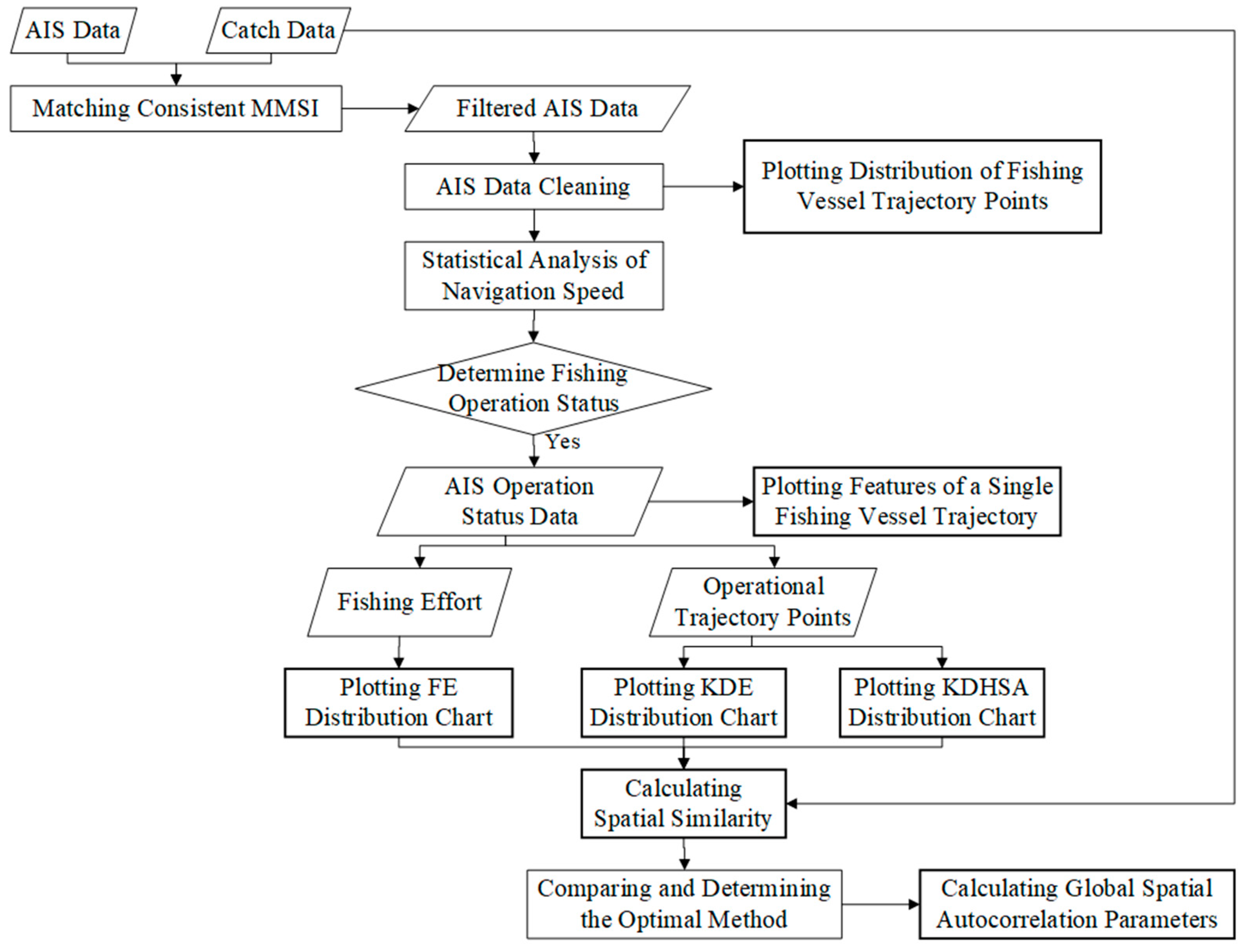
2.2.1. Technical Workflow

In this paper, the extraction method for fishing grounds was investigated using AIS data from mainland China’s purse seine fishing vessels operating in the Arabian Sea. As shown in Figure 2, the process is outlined in the following steps:

• The AIS data were compared with the relevant catch data and identity information of mainland China’s purse seine fishing vessels, and the AIS data corresponding to the MMSI numbers of the relevant fishing vessels were screened out.
• Data cleaning was conducted on the original AIS data following the method outlined in Section 2.1.2.
• The cleaned data were analyzed to identify AIS records indicating the fishing behavior of the fishing vessels and the trajectories of fishing vessel operations were extracted, which were visually represented as fishing vessel operation trajectories.
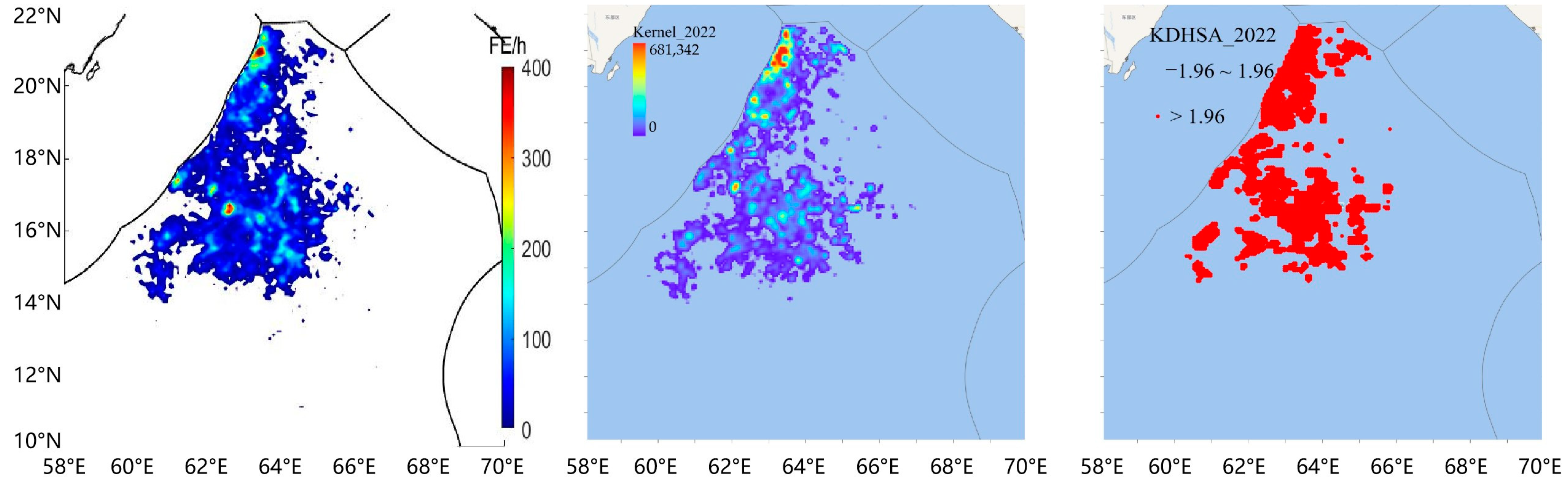
• Three methods, namely, fishing effort (FE), KDE, and kernel density hotspot analysis (KDHSA), were utilized to extract fishing grounds and subsequently, the results were compared and analyzed.
• The extraction results of the three methods were compared with the catch data, and a spatial similarity analysis was performed.
• The most effective method was determined and statistical analyses were conducted on the extracted fishery information, including global autocorrelation and other relevant parameters.

2.2.2. Operation Behavior of the Light Purse Seine Vessels

Light purse seine fisheries leverage the phototropic characteristics of small pelagic fish by utilizing fish-collecting lamps to attract them around fishing vessels at night for capture. During the day, fishing vessels may drift, travel at high speeds, or relocate to different fishing grounds. Light purse seine fishing vessel operations are characterized by notable variations in speed and time.

2.2.3. Identification of Fishing Vessel Operation Status

Light purse seine fishing vessels operate in a drifting state at night; therefore, in this paper, we used the solaR package (version 4.2.3) in R to calculate the solar radiance, defined a value of 0 as night, and combined this value with the speed of the fishing vessel to construct a trajectory point operation state identification model with the following formula:

$$P=\left\{\begin{array}{cc}1,\hfill & Bo0=0 and v_1<v<v_2 \\ 0,\hfill & else\end{array}\right.$$

(1)

where P denotes the fishing state and a value of 1 signifies fishing and 0 indicates nonfishing, Bo0 represents luminosity, $v$ signifies the speed of the fishing vessel, and $v_1$ and $v_2$ denote the upper and lower bounds of the speed threshold, respectively. The speed thresholds were determined using the Gaussian mixture model (GMM).

The time for each operation point is calculated as follows:

$${dt}_k=\left\{\begin{array}{cc}{t}_{k+1}-t_k\hfill & k=1\\ {\displaystyle \frac{\left(t_{k+1}-t_k\right)+\left(t_k-t_{k-1}\right)}{2}}\hfill & 1<k<n\\ t_k-t_{k-1}\hfill & k=n\end{array}\right.$$

(2)

where ${dt}_k$ represents the duration of the kth point in the extracted sequence of fishing vessel track points and $t_k$ denotes the update time of the kth track point in the extracted sequence. The interval time was calculated between the first track point and its neighboring subsequent point, as well as between the last track point and its preceding point.

Fishing intensity is defined as the cumulative operating hours in a single 0.1° × 0.1° latitude/longitude grid, expressed by the following equation:

$$E_{lon,lat}=\sum {dt}_{lon,lat}$$

(3)

where lon, lat represents the latitude and longitude, respectively, of the rasterized grid vertices of the map divided into 0.1° × 0.1°; $E_{lon,lat}$ signifies the fishing intensity; and ${dt}_{lon,lat}$ denotes the cumulative operating time of the grid track points.

The formula for calculating the center of gravity of the fishing effort is as follows:

$$FX={\displaystyle \frac{\sum _{i=1}^n\left(F_i\times X_i\right)}{\sum _{i=1}^n{F}_i}} ,FY={\displaystyle \frac{\sum _{i=1}^n\left(F_i\times Y_i\right)}{\sum _{i=1}^n{F}_i}}$$

(4)

where FX and FY represent the latitude and longitude, respectively, of the center of gravity of the fishing effort in each month; $X_i$ is the longitude of the ith grid in the fishing effort calculation; $Y$ is the latitude of the ith grid in the fishing effort calculation; n is the total number of grids; and $F_i$ is the fishing effort of the ith grid.

2.2.4. Kernel Density Estimation

KDE is a nonparametric method used to estimate probability density functions for calculating the density of an element in its surrounding neighborhood. The computational equation for kernel density estimation can be expressed as follows:

$$f\left(x\right)={\displaystyle \frac{1}{n{h}^d}}\sum _{i=1}^{n}K\left({\displaystyle \frac{1}{h}}\left(x-x_i\right)\right)$$

(5)

where $K$() is the kernel function, h is the bandwidth, n is the number of known points within the bandwidth, and d is the dimension of the data.

In this study, the kernel density tool in ArcGIS software (version 3.2) was used to calculate the intensity of the fishing activities of fishing vessels and their attenuation with distance. The spatial accuracy was set at 0.01° × 0.01°, and the temporal accuracy was monthly. The default value of the search radius was used. The kernel function utilized a Gaussian function to smooth the point density values in each cell with the values of adjacent cells. The resulting density surface was visualized using gradient colors to represent the point density in different regions.

2.2.5. Hotspot Analysis

The HSA is a local autocorrelation statistic employed to identify spatially hotspot areas in the distribution of fishing vessel activities. In the ArcGIS software, the hotspot analysis utilized Z scores, p values, and confidence intervals to generate a new output element class based on the input element class. A Z score greater than 1.96 indicates that the probability of an element being a hotspot is greater than 95%, with a higher Z score corresponding to a higher degree of hotspot aggregation. Conversely, a Z score of less than −1.96 indicates that the probability of an element being a coldspot is greater than 95%, and a lower Z score corresponds to a greater degree of coldspot aggregation. A Z score between −1.96 and 1.96 suggests that the element is most likely randomly distributed, lacking obvious statistical characteristics. In this study, a Z score of ±1.96 served as the threshold for delineating the hotspot area of fishing activities and the region with no obvious statistical characteristics. This was carried out to extract the range of the fishing activity aggregation area, and the hotspot area was visualized using gradient color or other visualization methods. The spatial accuracy was set at 0.01° × 0.01°, and the temporal accuracy was monthly.

2.2.6. Kernel Density Hotspot Analysis

KDHSA integrates KDE with HSA to identify the spatial distribution characteristics of fishing activities. In the ArcGIS software, this method identified hotspot and coldspot areas by combining the kernel density results with the local autocorrelation statistics. This study utilizes high-resolution grids and a monthly time frame, selecting a fixed distance as the weight coefficient. By incorporating the geographic units of kernel density values into the HSA method, it can successfully identify statistically significant spatial hotspots and extract fishing hotspot areas [22].

2.2.7. Spatial Similarity Statistics

Fishing grounds, calculated from fishery data, were compared with estimated fishing positions by computing the I similarity statistic [23]. This global metric accumulates the disparities between two predictions taken in pairs, yielding a single value that reflects the similarity of the two distributions based on their variable intensity and spatial distribution. The I similarity statistic varies between 0 (indicating no overlap between the two spatial distributions) and 1 (indicating identical spatial distributions).

2.2.8. Global Moran’s Index

The global autocorrelation Moran’s index is a statistical measure of the global spatial autocorrelation of spatial datasets. To comprehend the global spatial distribution pattern of fishing vessel operations in the Arabian Sea, the global Moran’s index (GMI) in spatial autocorrelation analysis was used as a metric with the following formula:

$$I={\displaystyle \frac{n{\sum }_{i=1}^n{\sum }_{j=1}^n{w}_{i,j}{z}_i{z}_j}{\left({\sum }_{i=1}^n{\sum }_{j=1}^n{w}_{i,j}\right){\sum }_{i=1}^n{z}_j^2}},\left(i\ne j\right)$$

(6)

In Equation (6), n denotes the number of samples; $z_i$ and $z_j$ are the deviations in the attributes of elements i and j from the mean of all the sample attributes, respectively; and $w_{i,j}$ is the spatial weight between elements i and j. If elements i and j are adjacent, $w_{i,j}=1$, and vice versa, $w_{i,j}=0$. Moran’s index ranges from −1 to +1, where −1 denotes a complete negative correlation, +1 indicates a complete positive correlation, and 0 indicates the absence of spatial autocorrelation. The GMI ranges from −1 to 1. A value greater than 0 indicates that the elements are clustered in the entire study area, with a higher value signifying a greater degree of clustered distribution. A value less than 0 indicates that the elements are discretely distributed throughout the entire study area, and the closer the value is to −1, the greater the degree of discrete distribution. If the value is equal to 0, the elements are randomly distributed. The GMI tool in ArcGIS returns a Z score and a p value, where a larger Z score suggests that the elements are clustered, and a smaller p value indicates that the spatial distribution pattern is less likely to be random.

3. Results

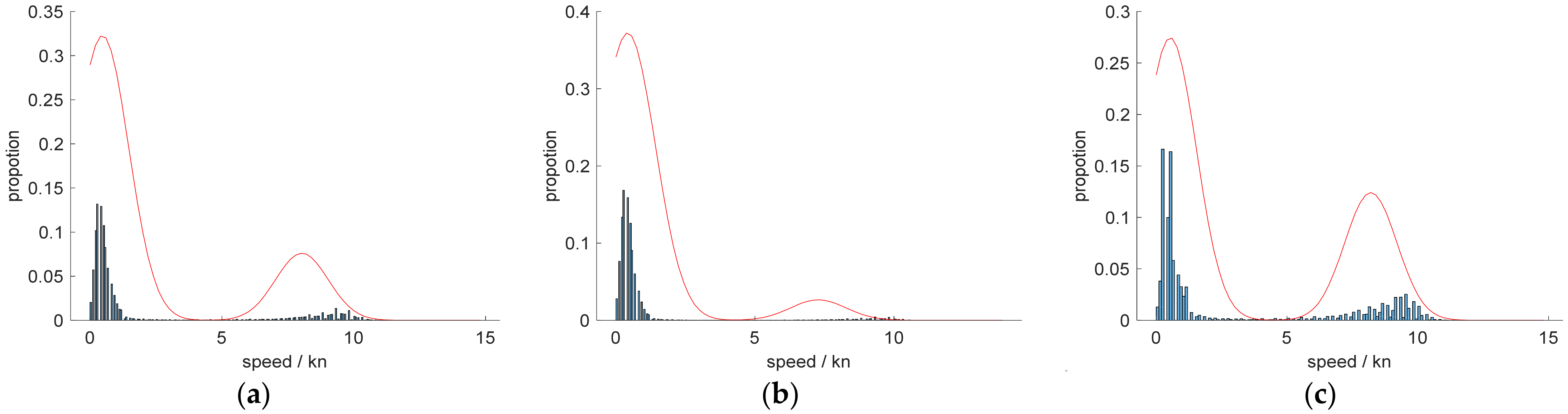
3.1. Analysis of Fishing Vessel Speed

The GMM curve-fitted velocity distribution plots (Figure 3) reveal a bimodal distribution of velocities for the all-day (Figure 3a), nighttime (Figure 3b), and daytime (Figure 3c) data during 2021 and 2022. The mean value of the first peak for the entire day data was 0.47 kn, with a standard deviation of 0.28. The nighttime data (Figure 3b) indicated that the mean value of the first peak was 0.42 kn, with a standard deviation of 0.24, suggesting that the fishing vessels operating at night were slowing down and in a drifting state. The daytime data (Figure 3c) showed that the mean value of the first peak was 0.53 kn, with a standard deviation of 0.32, which was slightly greater than the distribution of the first peak speeds of operational daytime fishing vessels. The distribution of the first peak speeds of fishing vessels during the day was slightly greater than that at night. All three plots consistently showed that the first peak speed was mostly below 1.5 kn, and this paper defined 1.5 kn as the upper limit of the speed threshold for the operating conditions of fishing vessels.

3.2. Analysis of Single Fishing Vessel Behavior

Figures S1 and S2 illustrate the speed trajectories and residence time distributions of the light purse seine vessel with MMSI No. 412440745 for 2021 and 2022. The speed plots (Figures S1a and S2a) show that the trajectory of the light purse seine vessel primarily comprises medium-speed points, with some instances of low-speed points. The spatial plots of the dwell times (Figures S1b and S2b) reveal that the light purse seiners exhibited prolonged dwell times in specific areas and brief dwell times at certain trajectory points. Additionally, the analysis indicated that these vessels engaged in extended dwell time after a period of moderate-speed travel to an area, proceeding to move at low speeds in that area before resuming prolonged dwell time. The spatial maps of operation time (Figures S1c and S2c) show that the extended dwell time and the dense concentration of trajectory points within specific sea areas suggest potential richness in fishery resources, indicating that significant large-scale fishing activities may have occurred there. Conversely, the short dwell time in other areas implies relatively low fishery resources, suggesting that vessels may have merely traversed through or conducted relatively brief fishing operations in those locations.

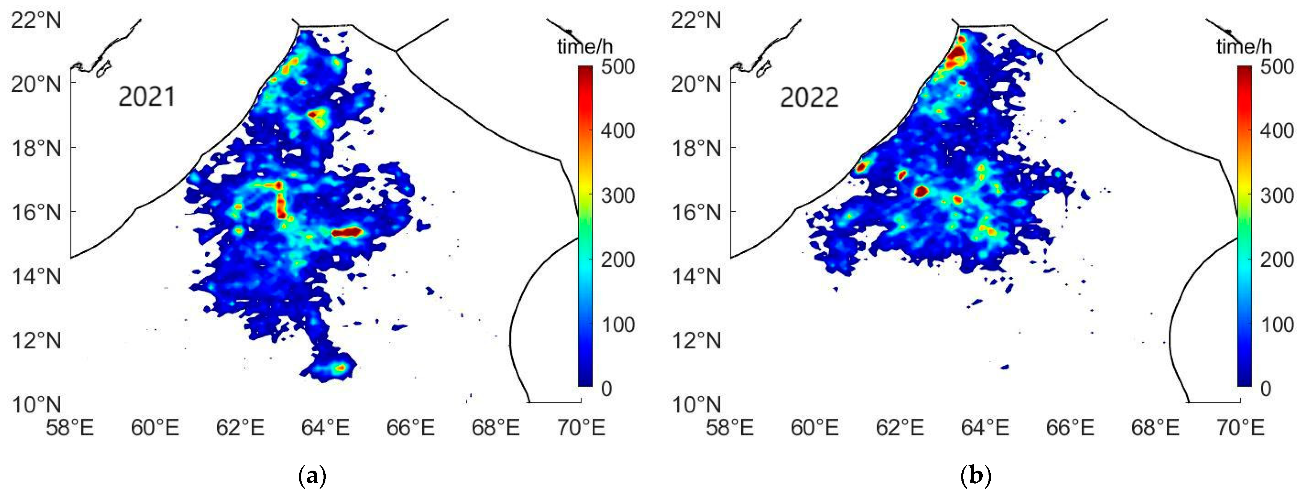
3.3. Spatial Distribution of Fishing Vessel Tracks

Figure 4 presents spatial maps illustrating the cumulative time of occurrence (without distinguishing between operational and non-operational periods) of all the fishing vessels in each grid for 2021 and 2022. The findings revealed that throughout the year, fishing vessel activity predominantly occurred near the southern high seas where the EEZ of Oman and the EEZ of Pakistan intersect. Several patchy areas with a high cumulative time of vessel occurrence were observed. Upon comparing 2021 and 2022, it became apparent that the majority of the areas with high cumulative times of vessel occurrence in both years did not coincide. Only a few areas exhibited consistently high cumulative times in both years. For instance, fishing vessels showed high cumulative times near the coordinates of 64°12′ E, 15°18′ N, and 63°24′ E, 21° N during both years.

The distribution of vessel trajectory points by month (depicted in Figure S3) revealed discernible seasonal variations in vessel activity. Notably, the area at approximately 64° E, 16° N exhibited a consistent year-round aggregation of vessel activity, suggesting heightened resource richness in this region. The spatial maps of trajectories for January, May, October, and November illustrate sailing departures from and arrivals at the fishing grounds. Specifically, in May, all the vessels left the operational area, while in October and November, almost all the vessels entered the fishing grounds. In November, virtually all the vessels accessed the fishing grounds, indicating a concentrated period of increased fishing activity.

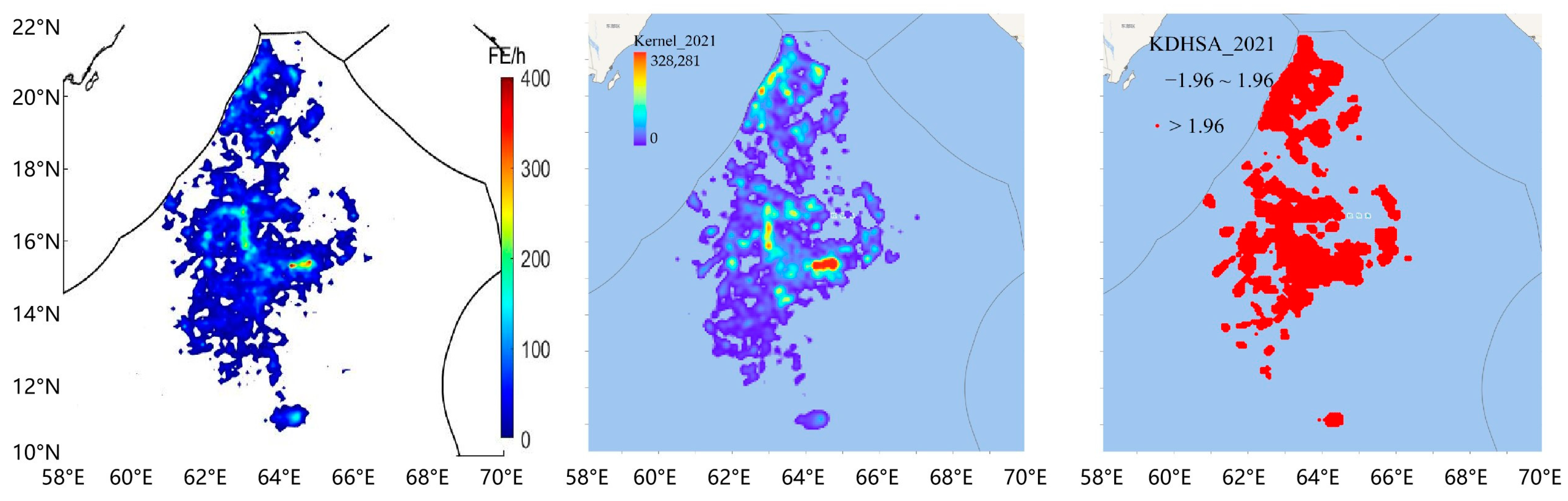
3.4. Comparison of the Mapping Results of Different Methods

Based on the results obtained from identifying the operational status of fishing vessel track points, calculations and mapping were performed to determine the distribution of fishing intensity, nuclear density, and hotspot spatial information. Figure 5 and Figure 6 show that the spatial distributions of fishing vessel operations, as mapped by the three methods, exhibited striking similarities. The spatial distribution of fishing vessel operations revealed a distinct patchy pattern, primarily concentrated in proximity to the Omani EEZ domain. Notably, small patches with high fishing intensity were observed in the study area, particularly at the coordinates 64°12′ E–64°42′ E, 15°18′–15°24′ N in 2021 and at the coordinates 63°18′ E–63°24′ E, 20°48′°–21° N and 62°30′ E–62°36′ E, 16°30′–16°42′ N. The cumulative fishing operation time of vessels per unit area within these high-intensity patches generally ranged between 200 and 500 h. Large areas with null values were interspersed between these high-value patches. Furthermore, other operational areas displayed diverse distributions. Noteworthy examples include 62°54′ E, 15°54′–16°42′ N and 63°42′ E, 19° N in 2021, as well as 61°6′–61°18′ E, 17°18′–17°30′ N and 63°18′–63°24′ E, 16°18′–16°24′ N in 2022, with the cumulative fishing operation times per unit area primarily falling within a range of 200–300 h. Similarly to the high-intensity patches, null-value areas were prevalent between these regions. Most regions exhibited an operating time of less than 100 h, with an average length of operation ranging between 200 and 300 h. In many areas, the average length of operation was approximately 100 h or less.

The spatial distribution patterns of purse seine fishing activities, as delineated by the three methods, exhibited notable distinctions (see Figure 5 and Figure 6). All three methods indicated that the fishing activities in the Arabian Sea occurred within a range of 4°–8° in both latitude and longitude. However, for certain small patches, the maps derived from the fishing effort and kernel density analyses depict a slightly larger and more detailed area compared to the hotspot analyses. The edges of the fishing intensity maps exhibit relatively sharp contrasts, while the edges of the hotspot map images appear smoother. The fishing effort and kernel density methods effectively captured both the high-density and low-density areas of fishing vessel operations. In contrast, the hotspot spatial information extracted by the KDHSA primarily reflected boundary information without distinguishing between the high-density and low-density areas. Consequently, the KDHSA was deemed unsuitable for evaluating fishing pressure on the fishing grounds. Fishery fishing effort maps prove more adept at illustrating the distribution of high and low values, featuring fewer clustered blocks, albeit with clearer boundaries and finer distributions.

Figure 7 shows the average spatial similarity indices of the fishery data and fishing intensity information at various spatial resolutions. The average spatial similarity indices consistently surpassed 0.7 when considering spatial accuracies greater than 0.2°. Notably, at spatial scales exceeding 0.2°, the spatial distributions of fishery data and fishing intensity information exhibited notable similarities, indicating a robust correspondence between the two datasets.

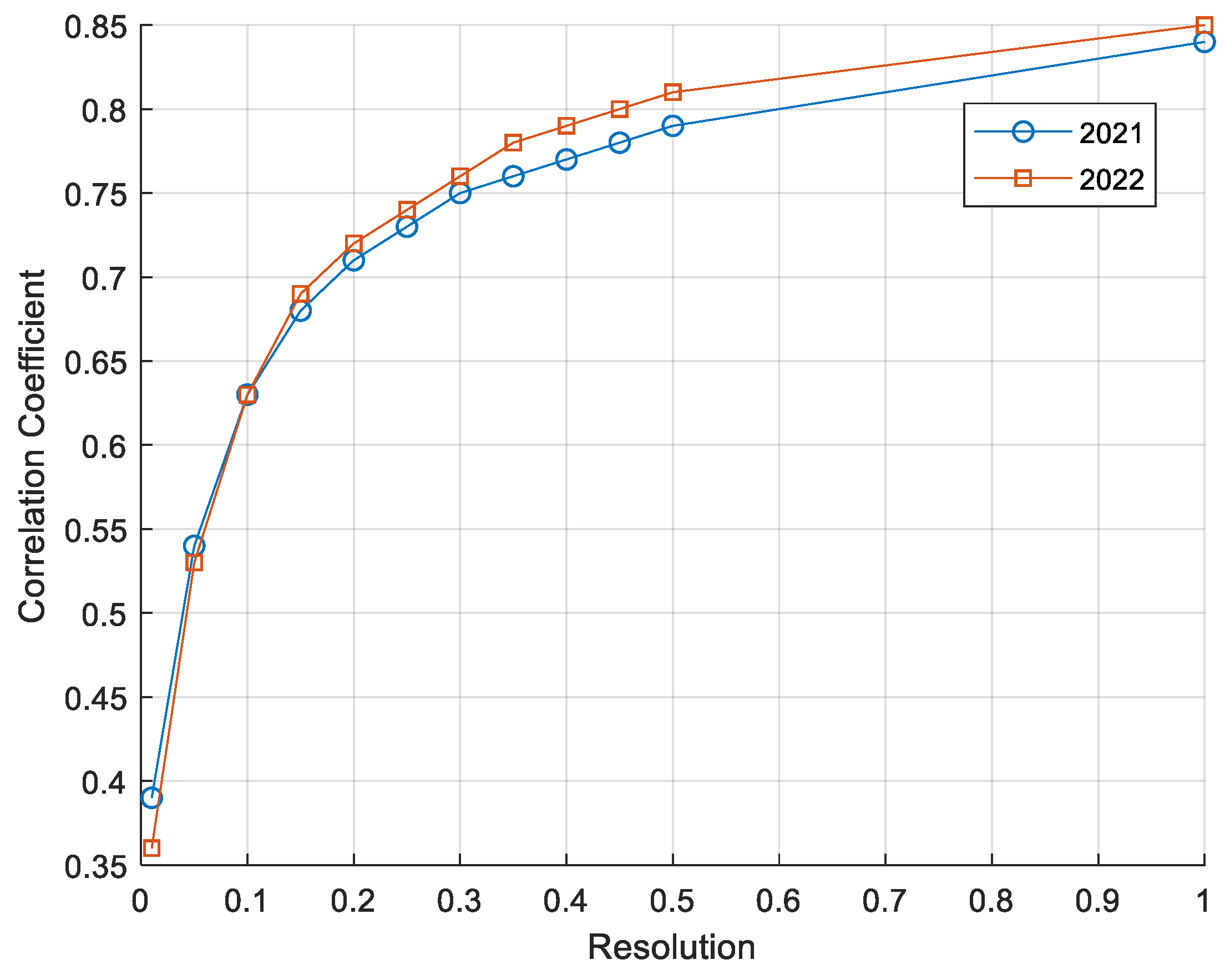
3.5. Spatial Similarity Index

Figure S4 presents spatial maps illustrating light purse seine catches in the Arabian Sea of the Indian Ocean for 2021 and 2022, with a spatial resolution of 0.25° × 0.25°. The spatial distribution of the annual catch data closely mirrors the spatial distribution of the annual fishing intensity. The catch maps reveal a distinct meridional trend characterized by interspersed high and low catches. Notably, the catch data were predominantly concentrated in the peripheral areas of the Omani EEZ, while minimal to no catches were observed near the Indian EEZ line. This spatial distribution underscores a clear trend in light purse seine catches within the specified region.

Table 1. Indicators of spatial similarity between the extraction results and the actual data by the three methods in 2021.

Method	Jan.	Feb.	Mar.	Apr.	May	Oct.	Nov.	Dec.
FE	0.7	0.7	0.76	0.71	0.65	0.75	0.76	0.74
KDE	0.7	0.69	0.74	0.71	0.65	0.46	0.72	0.7
KDHSA	0.59	0.55	0.59	0.56	0.52	0.69	0.54	0.52

and

Table 2. Indicators of spatial similarity between the extraction results and the actual data by the three methods in 2022.

Method	Jan.	Feb.	Mar.	Apr.	May	Oct.	Nov.	Dec.
FE	0.71	0.73	0.75	0.73	0.69	0.78	0.79	0.77
KDE	0.69	0.71	0.74	0.69	0.68	0.69	0.68	0.72
KDHSA	0.62	0.64	0.71	0.67	0.68	0.63	0.6	0.66

present the spatial similarity index between the fishing effort (FE) information extracted using the three methods and the catch data from actual production operations, considering a spatial accuracy of 0.25° × 0.25° for the periods of January–May and October–December. In 2022, the spatial similarity indices between the FE extracted via the three methods and the catch data consistently exceeded 0.60 for all three methods. Notably, in 2021, the spatial similarity index was highest at 0.76, and this value increased to 0.79 in 2022. For specific months, the spatial similarity index peaked at 0.76 in March 2021 and reached 0.79 in November 2022. In March 2022, the spatial similarity indices calculated using all three methods were consistently greater than 0.71. Upon comparing the three methods, it was observed that the spatial similarity indices between the fishery information extracted using KDHSA and the catch data from actual production operations were the lowest. Additionally, the spatial similarity index between the FE and catch data from actual production operations was the lowest for KDHSA, while it was the highest for the other two methods.

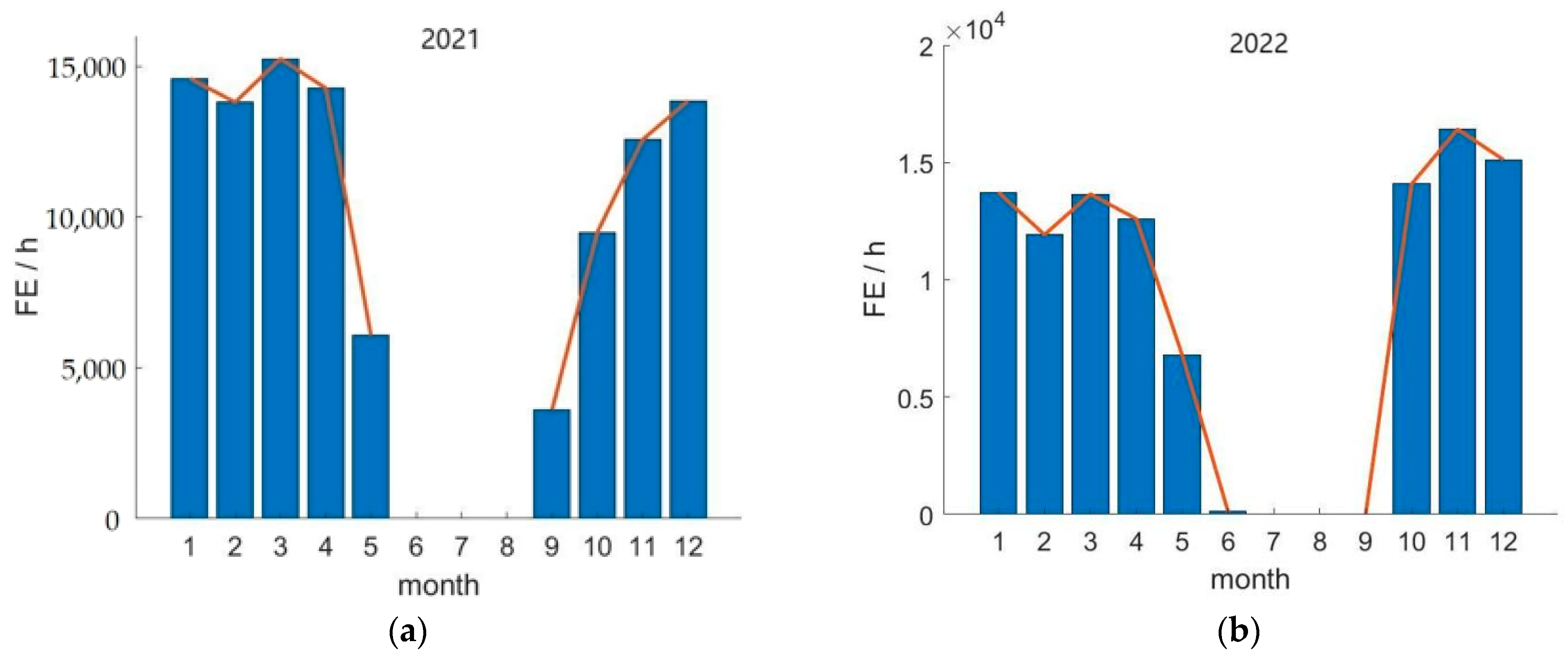
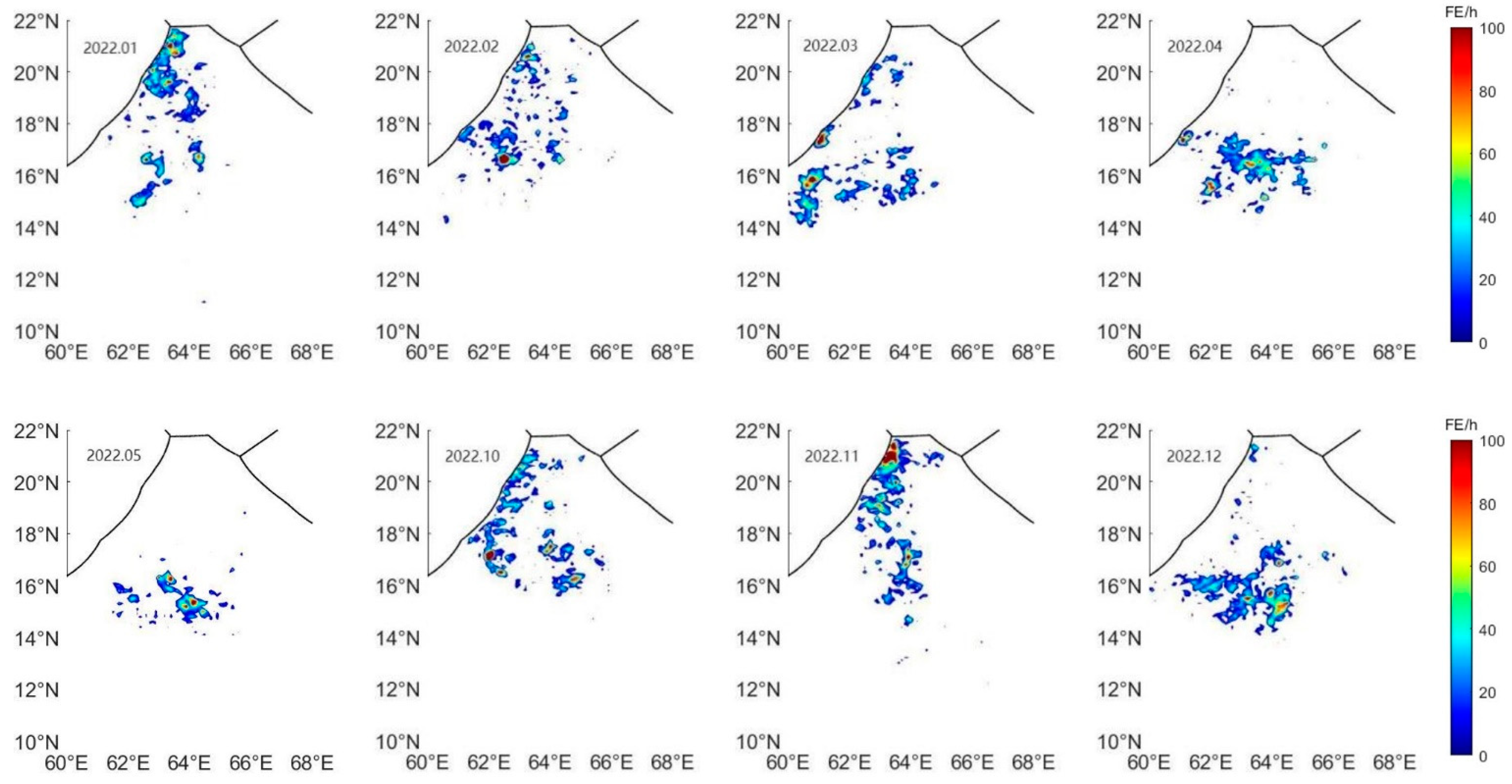
3.6. Characterization of the Spatial Distribution of Fishing Vessel Operations

The monthly distribution of fishing effort by mainland China’s light purse seine vessels in the Arabian Sea in 2021 and 2022 is illustrated in Figure 8. The statistics revealed that fishing effort was primarily concentrated from January to May and from October to December. Among these, January and March had the highest levels, while September had the lowest, with almost no fishing vessel operations observed from June to August. The following analysis focuses on January to May and October to December.

Due to the optimal spatial alignment between fishing effort and production data, fishing intensity was utilized to analyze the spatial distribution characteristics of fishing vessel operations. The monthly distribution of fishing intensity for 2021–2022 is visually represented in Figure 9 and Figure 10. The spatial intensity maps for each month reveal the patchy nature of the spatial distribution of fishing vessel operations. The distribution was characterized by discrete patterns, with no contiguous areas of concentrated operations. However, small yet highly concentrated areas were consistently present each month, with cumulative time exceeding 100 h in a 0.1° × 0.1° area. Notably, certain months exhibited maximum cumulative times ranging from 200 to 350 h, indicating highly aggregated fishing activities in those periods. The spatial distribution of fishing effort displayed significant monthly variations, highlighting distinct seasonal changes.

In Figure 9 and Figure 10, the areas with the duration of fishing effort per month in 2021 and 2022 were assessed at a resolution of 0.1° × 0.1°. In October 2021, a peak concentration was observed at 63° E, 15°54′ N, lasting for up to 322 h. Subsequently, in February 2022, another concentration was recorded at 62°30′ E, 16°42′ N, lasting for up to 350 h. These findings suggest that fishing vessels had identified a substantial abundance of fishery resources in these areas. These monthly observations provide us with valuable insights into the dynamic utilization of fishing resources.

3.7. Centre of Gravity of Fishing Vessel Operations

Due to the optimal spatial alignment between fishing effort and production data, this study employed fishing effort information to calculate the center of gravity of fishing vessel operations. Figure S5 illustrates the evolution of the center of gravity of fishing effort for light purse seine vessels from January to May and October to December 2021 and 2022. In 2021, the overall center of gravity of fishing effort exhibited a gradual shift from low to high latitudes from January to May. Specifically, it moved from high to low latitudes from January to February, from low to high latitudes from February to April, and from high to low latitudes from April to May. The center of gravity was greater in latitude in October. From October to November, it shifted slightly from low to high latitude, and from November to December, it moved from high latitude–high longitude to low latitude–low longitude. In 2022, the spatial and temporal changes in the center of gravity of fishing effort from January to May differed significantly from those in the same period in 2021. However, the pattern from October to November in 2022 mirrored that of 2021. Notably, from January to May in 2022, the center of gravity gradually shifted from high latitudes to low latitudes, opposite to the trend observed in 2021. From October to December 2022, the vessel movement pattern remained consistent with that of 2021.

The comparable centre of gravity between 2021 and 2022 from October to December underscores a consistent trend in vessel movement during those months. The observed shifts in the center of gravity provide valuable insights into the evolving fishing activity of light purse seine vessels across different months.

3.8. Global Spatial Pattern of Fishing Vessel Operations

As indicated in Tables S1 and S2, the mean fishing effort was consistently greater in October and November of each year. The maximum mean value occurred in December 2021, followed by March 2021, while lower values were observed in December and March 2022. The mean fishing effort in the fishing area was smallest in May 2021, with a similarly smaller value in May 2022. Skewness values for all the months were greater than 0, revealing a positively skewed frequency distribution, indicating a prevalence of lower values with fewer instances of high values. Kurtosis values exceeding three further emphasized that the squid fishing effort in the study area was dominated by low values. The coefficient of variation for each month surpassed one, signifying a strong variance and indicating a substantial variation in fishing effort within the study area. The results from the GMI indicated that while the index for each month was greater than 0, they were all relatively small. This suggests a weak positive spatial correlation in fishing effort across months. High Z scores and p values less than 0.01 further indicated spatial aggregation in the distribution of fishing effort by fishing vessels each month, affirming that it was not a randomly distributed phenomenon. This observation is consistent with the identified small areas of highly concentrated effort illustrated in Figure 9 and Figure 10.

4. Discussion

4.1. The Reliability of AIS Data

It is crucial to consider the potential impact of AIS transmission rates on the overall data quality and accuracy in assessing fishing vessel activities. Mainland China’s purse seine fishing vessels are active in the high seas of the North Pacific Ocean, the Western Pacific Ocean, the Southwest Atlantic Ocean, and the Indian Ocean. To better safeguard and optimize the utilization of fishery resources on the high seas, China’s fisheries management authorities have implemented management measures for the areas where purse seine fishing vessels operate. Consequently, only authorized vessels are permitted to operate in the Arabian Sea of the Indian Ocean. The potential reasons for missing data from these vessels may include AIS equipment malfunctions or the captain’s decision to deactivate the equipment, leading to a potential underestimation of fishing effort. It is recommended to enhance the security of the existing AIS using encryption technology to protect signals, or to introduce multi-factor authentication mechanisms to reduce the risk of the transmitters being turned off. Additionally, it is worth noting that an increase in vessel density can impact the reception quality of AIS signals. Signals are susceptible to interference and attenuation in high-density waters, resulting in a decrease in signal quality. Recognizing the importance of accurate data, China’s fishery administration has recently mandated that fishing vessels operating on the high seas must ensure that their AIS equipment is activated. This proactive measure is expected to contribute to more precise and comprehensive data for fishery analysis and management in the future.

Due to the limitations of the collected AIS data, we only analyzed the spatial distribution characteristics of fishing vessel operations for 2021–2022. However, this paper clearly outlines appropriate methods and spatial scales.

4.2. Fishing Vessel Operational Status Recognition

Accurately determining the operational state of fishing vessels holds paramount importance in fishing spatial information mining. Typically, the sailing speed of fishing vessels is employed to ascertain their operational state, a method widely used in the literature [24,25]. However, the definition of speed thresholds often relies on expert knowledge and statistical modeling [11,14,15]. While this approach is efficient, especially for vast fishing vessel trajectories, it has limitations, as the operational status is influenced by various factors. The statistical findings in this study revealed a notable number of low-speed trajectory points during the daytime. Importantly, light purse seines generally do not operate during daylight hours. Failing to differentiate between daytime and nighttime information can lead to an overestimation of fishing effort and fishing pressure in the fishery, potentially misguiding fisheries research and management. To address this issue, this study utilized the Solar R package to calculate solar radiance, defining trajectory points with a solar radiance of 0 as nighttime trajectory information. Further analysis of the bimodal distribution of fishing vessel speeds shows that daytime speed distribution is slightly higher than at night. This is expected, as clearer visibility during the day allows for more flexible and efficient operations. By examining speed distributions across the entire day, nighttime, and daytime, we found that the first peak speed across all the time periods is primarily below 1.5 kn. This observation enables us to clearly define 1.5 kn as the upper threshold for fishing vessel operational speed. The bimodal distribution phenomenon and the differences in speed distribution across different times of day provide important insights for identifying fishing activities during various periods. This information serves as a valuable reference for optimizing fishery management and resource conservation strategies, enhancing the scientific monitoring and management of fishing activities. Additionally, the exploration of deep learning for fishery operation state recognition has shown promising results. Future endeavors should involve the integration of deep learning methods with field survey data to enhance the accuracy of fishing vessel operation state recognition models. This approach holds the potential for improving the precision and reliability of identifying fishing vessel operational states in practical applications.

4.3. Comparison of the Three Methods for Extracting Spatial Information and Spatial Similarity Analysis

Spatial variations in the maps were evident due to methodological factors; however, the fishing grounds extracted by the three methods exhibited overall consistency, were primarily located near the Omani EEZ domain, and displayed characteristic patchy distributions. Notably, the spatial similarity index between the fishing ground information extracted by the FE methods and the catch data from actual production operations was the highest, while KDHSA showed the lowest similarity. This suggests that KDHSA introduced some divergence in the spatial characterization compared to the actual production operation, highlighting a nuanced difference. The spatial distribution of fishing intensity and the spatial distribution of production data for each month demonstrated the highest compatibility. In October 2021, the similarity index calculated by KDE was 0.46, potentially indicating a lack of catch due to unknown fishery resources in the Arabian Sea. This anomaly was likely associated with vessels engaging in prolonged salvage operations in that region.

Theoretically, when analyzing fishing vessel track data, the possibility of dividing time and space at a fine granularity exists. However, the determination of appropriate spatial and temporal scales is crucial and should align with the specific objectives of the study. The average spatial similarity index of fishery data and fishing intensity information at different spatial resolutions indicated that a spatial scale of 0.2° achieved an average similarity index exceeding 0.7. Considering that the 0.25° spatial scale also consistently surpassed 0.7 for all the months, it was deemed more reasonable for statistical analyses in the Arabian Sea, striking a balance between spatial accuracy and similarity to fishery resources. Excessive spatial precision can pose challenges to fisheries management and analysis. Figure S6 illustrates the fishing effort intensity at a high resolution, 0.01° × 0.01°, displaying dense and discrete areas resembling scattered sands in densely packed regions. To mitigate this, a map of fishing intensity at a resolution of 0.1° × 0.1° was developed in this study. Additionally, the maps for the kernel density and hotspot analysis were generated at a spatial resolution of 0.05° × 0.05°, providing smoother raster outputs. This higher resolution contributed to more comprehensive and detailed results in the analysis.

Chen et al. [15] highlighted that KDHSA leverages the strengths of both KDE and HSA, integrating the distance decay effect of KDE [26] with the statistical index of HSA [27]. However, the hotspot map generated by KDHSA did not include information on coldspots, resulting in a lower spatial similarity index than that of the other methods. Spatially, the hotspots extracted by KDHSA could only reveal boundary information and lacked the representation of both high-density and low-density areas. This limitation hindered the ability to showcase the changing spatial distribution of the fishery, making KDHSA unsuitable for assessing fishery pressure. Despite exhibiting sharper boundaries, the fishery intensity map demonstrated the highest spatial similarity index and clearly illustrated the spatial distribution characteristics. The kernel density map, while displaying the spatial variability of the fishery with smooth boundaries, did not perform as well overall as the fishery intensity map.

4.4. Spatial and Temporal Distribution of Fishing Vessel Operations

Light purse seine vessels in the Arabian Sea of the Indian Ocean exhibited heightened activity during the first and fourth seasons, with the primary fishing period spanning from late September to May of the following year. This is consistent with the occurrence of the northeast monsoon in the Indian Ocean, indicating continuous operation by mainland China’s light purse seine fishing vessels throughout the year in this region. Spatially, the distribution of fishing vessel operations formed a distinct patchy pattern, predominantly close to the Omani EEZ area. The notable areas of high fishing intensity were concentrated in the study area, with the spatial clustering of fishing vessel operations observed at 60°–68° E, 15°–20° N. The spatial similarity index test results affirm that the spatial information extracted by the three methods closely aligns with the distribution and movement trends of the fishing grounds.

There is a potential correlation between the center of fishing effort and the ecological and environmental factors in the Arabian Sea. Firstly, ocean temperature is a significant factor influencing the center of fishing effort. The ocean temperature in the Arabian Sea varies significantly with the seasons; in winter, when the water temperature is lower, fishing vessels may migrate to warmer waters, whereas in summer, with rising temperatures, they may move to cooler areas. From January to May 2021, the center of the fishing effort gradually shifted from lower to higher latitudes, and from October to December, it remained at higher latitudes, closely linked to the seasonal temperature changes. In contrast, from January to May 2022, the center moved from higher to lower latitudes, opposite to the pattern in 2021, but the movement from October to December was consistent with 2021, demonstrating the impact of seasonal temperatures on fishing activities. Secondly, ocean productivity also plays a crucial role in influencing the center of fishing effort. Ocean productivity directly affects fish growth and distribution, with the areas of high primary productivity typically attracting more fishing vessels. The abundance of phytoplankton and nutrient supply in the Arabian Sea are significantly influenced by monsoons and ocean currents. The rainfall and nutrients brought by the southwest and northeast monsoons promote changes in ocean productivity, thereby affecting the spatial distribution of fishing effort. A high coefficient of variation (Cv > 1) and a global Moran’s I index (Moran’s I > 0) indicate that squid fishing activities exhibit significant spatial clustering rather than random distribution, which is highly correlated with the spatial distribution of ocean productivity. Overall, the seasonal and spatial movement of the center of fishing effort partially reflects the significant impact of the ecological and environmental factors in the Arabian Sea on fishing activities.

The considerable variability observed in the fishing vessel operating spaces across different months indicates substantial seasonal fluctuations in fishery resources within the region. The existing research has focused primarily on analyzing the relationships between resource variations and environmental factors during the fishing season [28]. However, there is a significant gap in the understanding of the migration patterns and routes of key catch species, such as squid and mackerel, in this particular sea area. Current studies have not fully elucidated these migration dynamics. Addressing this gap will require further observations and survey studies. More comprehensive research efforts in the future will contribute to understanding the migratory behavior of major catch species, providing invaluable data for a deeper comprehension of the ecosystems within this sea area.

4.5. Implications for Fisheries Management

The mapping of fishing intensity, kernel density, and hotspots revealed a patchy spatial distribution of fishing vessel operating spaces in the Arabian Sea. Within this region, high-value patches were interspersed with 0 value patches, as confirmed by the spatial distribution map of the catch data. This patchy distribution underscores the need for fine-grained fisheries and environmental data for effective resource analysis and management in the area. Greater spatial precision in the analysis may smooth detailed information about resource distribution and potentially lead to misleading conclusions.

In the patchy spatial distribution phenomenon, the substantial spatial variation in operations across different months underscores the considerable seasonal fluctuation of the fishery resources in the region. Simultaneously, the global spatial analysis, as illustrated in Table 2, indicated a non-random distribution, revealing spatial aggregation in the monthly distribution of fishing vessels engaged in catches. This suggests that despite the notable month-to-month variability in the spatial distribution of fishing vessel operations, a majority of these vessels tended to operate in clusters, particularly those affiliated with the same fishing vessel production enterprises. The patchy and spatially clustered nature of fishing vessel operating spaces highlights significant changes in the region’s fishery, emphasizing that fishing vessels have yet to fully grasp the characteristics of fishery distribution and its changing patterns. Effective fishery management necessitates a comprehensive understanding of the migration and distribution of fishery resources in the region. Given that the light purse seine fishery in the area borders the exclusive economic zones of multiple countries, it becomes imperative to strengthen international cooperation in regional fishery resource management. This cooperation should focus on comprehending the migratory paths and biological habits of fishery resources in the region, establishing an effective joint fishery management mechanism, and enhancing the regulation of the fishing vessels operating in the area.

The statistical analysis presented in this paper revealed a notable decline in fishing vessel operations during the period from June to September, consistent with the findings from previous fishery data studies [18,19]. Mainland China’s fishing vessels traditionally embark on fishing expeditions in September for annual operations. Notably, the fishing season in the Arabian Sea spans from October to May of the following year. Notably, engaging in fishing operations during non-fishing seasons can have severe detrimental effects on fishery resources [29]. Commencing in 2020, China implemented a high-sea fishing moratorium policy, which was effective from July 1 to September 30. In 2022, the high sea waters of the northern Indian Ocean (55° E–70° E, 0° N–22° N), excluding the SIOFA jurisdictional area, were also included in the high sea closure area, as corroborated by the absence of fishing effort in September 2022, as depicted in Figure 8. The methodology outlined in this paper demonstrates that AIS vessel position data can serve as a valuable tool for monitoring the potential violations of regulations during closed seasons. While the AIS data for 2021–2022 in this study are somewhat limited, the applied methodology serves as a viable model for future studies.

Moreover, inherent limitations in AIS data contribute to challenges such as short-term information gaps resulting from the brief artificial shutdowns of AIS equipment. Distinguishing this situation from data loss due to transmission issues is complex. Bernabé et al. [30] utilized self-supervised deep learning techniques and transformer models to detect abnormal intentional AIS transponder shutdowns. Light purse seine fishing vessels operating in the Arabian Sea are in close proximity to the EEZs of numerous countries, with some vessels operating along these EEZs. While China’s fisheries administration mandates that fishing vessels operating on the high seas keep AIS equipment operational, the absence of AIS information is a global reality for fishing vessels. The unrecorded fishing vessel activity contributed to an additional 19% (5500 h) of the activity by AIS-equipped fishing vessels between 2017 and 2022 in the Northeast Pacific [31]. Given the difficulty in identifying AIS information for short durations, it becomes imperative to enhance the supervision and regulation of fishing vessels by integrating other technical methods. Incorporating tools such as night-light remote sensing [32], synthetic aperture radar (SAR) image data, aerial surveillance (“flyovers”) [33], and remote sensing radio information is essential for establishing a comprehensive supervision system for the operational behavior of fishing vessels. This integrated approach aims to achieve more effective management of fishing vessel operations.

5. Conclusions

In this study, the distribution of spatiotemporal information related to the operations of light purse seine fishing vessels in the Arabian High Seas was extracted and subjected to spatial analysis based on AIS data. The findings present a methodological framework for comprehending information pertaining to fishing vessel operating patterns, areas under fishing pressure, and seasonal variations. The following conclusions were drawn:

• The spatial distributions of fishing effort and kernel density were similar to the spatial layout of fishing grounds. The spatial similarity between fishing effort and catch data was the highest, with the use of a 0.25° spatial scale deemed most suitable for extracting and analyzing spatial information related to light purse seine fishing vessels in the Arabian Sea.
• The operational space of light purse seine fishing vessels in the Arabian Sea displayed patchy distribution characteristics and underwent significant spatial changes each month. There were evident seasonal variations with no apparent distribution pattern, emphasizing the need for detailed information in resource analysis and management within this region.
• AIS data were valuable for monitoring the operations of light purse seine fishing vessels in the Arabian Sea. Through real-time data supervision, it enhanced the monitoring of fishing ground distribution and fishing pressure, assisting in global resource conservation efforts. However, it is essential to integrate other technical methods for more effective supervision of fishing vessel operations.

References

1. Chen, R.; Wang, Y.; Wu, X.; Gao, Z. Identifying the Key Factors Influencing Spatial and Temporal Variations of Regional Coastal Fishing Activities. Ocean Coast. Manag. 2024, 248, 106940. [Google Scholar] [CrossRef]
2. Tickler, D.; Meeuwig, J.J.; Palomares, M.-L.; Pauly, D.; Zeller, D. Far from Home: Distance Patterns of Global Fishing Fleets. Sci. Adv. 2018, 4, eaar3279. [Google Scholar] [CrossRef] [PubMed]
3. Xu, Z.; Wang, J.; Zhou, C.; Lei, L.; Chen, X.; Li, B. Identification of Fishing State of Purse Seine Fishing Vessels Based on Multi-Indices. J. Ocean. Univ. China 2023, 22, 1605–1612. [Google Scholar] [CrossRef]
4. Mullié, W.C. Apparent Reduction of Illegal Trawler Fishing Effort in Ghana’s Inshore Exclusive Zone 2012–2018 as Revealed by Publicly Available AIS Data. Mar. Policy 2019, 108, 103623. [Google Scholar] [CrossRef]
5. Cimino, M.A.; Anderson, M.; Schramek, T.; Merrifield, S.; Terrill, E.J. Towards a Fishing Pressure Prediction System for a Western Pacific EEZ. Sci. Rep. 2019, 9, 461. [Google Scholar] [CrossRef]
6. Kroodsma, D.A.; Mayorga, J.; Hochberg, T.; Miller, N.A.; Boerder, K.; Ferretti, F.; Wilson, A.; Bergman, B.; White, T.D.; Block, B.A.; et al. Tracking the Global Footprint of Fisheries. Science 2018, 359, 904–908. [Google Scholar] [CrossRef]
7. Vespe, M.; Gibin, M.; Alessandrini, A.; Natale, F.; Mazzarella, F.; Osio, G.C. Mapping EU Fishing Activities Using Ship Tracking Data. J. Maps 2016, 12, 520–525. [Google Scholar] [CrossRef]
8. Russo, E.; Monti, M.A.; Mangano, M.C.; Raffaetà, A.; Sarà, G.; Silvestri, C.; Pranovi, F. Temporal and Spatial Patterns of Trawl Fishing Activities in the Adriatic Sea (Central Mediterranean Sea, GSA17). Ocean Coast. Manag. 2020, 192, 105231. [Google Scholar] [CrossRef]
9. Yan, Z.; He, R.; Ruan, X.; Yang, H. Footprints of Fishing Vessels in Chinese Waters Based on Automatic Identification System Data. J. Sea Res. 2022, 187, 102255. [Google Scholar] [CrossRef]
10. James, M.; Mendo, T.; Jones, E.L.; Orr, K.; McKnight, A.; Thompson, J. AIS Data to Inform Small Scale Fisheries Management and Marine Spatial Planning. Mar. Policy 2018, 91, 113–121. [Google Scholar] [CrossRef]
11. Wang, Y.B.; Wang, Y. Estimating Catches with Automatic Identification System (AIS) Data: A Case Study of Single Otter Trawl in Zhoushan Fishing Ground, China. Iran. J. Fish. Sci. 2016, 15, 75–90. [Google Scholar]
12. Lee, J.; South, A.B.; Jennings, S. Developing Reliable, Repeatable, and Accessible Methods to Provide High-Resolution Estimates of Fishing-Effort Distributions from Vessel Monitoring System (VMS) Data. ICES J. Mar. Sci. 2010, 67, 1260–1271. [Google Scholar] [CrossRef]
13. Sun, Y.-W.; Zhang, S.-M.; Tang, F.-H.; Wang, S.-X.; Fan, W.; Fan, X.-M.; Yang, S.-L. Research on the Distribution and Types of Fishing Vessels in the North Pacific Based on Satellite Ship Position Data. J. Agric. Sci. Technol. 2022, 24, 207–217. [Google Scholar]
14. Le Guyader, D.; Ray, C.; Gourmelon, F.; Brosset, D. Defining High-Resolution Dredge Fishing Grounds with Automatic Identification System (AIS) Data. Aquat. Living Resour. 2017, 30, 39. [Google Scholar] [CrossRef]
15. Chen, R.; Wu, X.; Liu, B.; Wang, Y.; Gao, Z. Mapping Coastal Fishing Grounds and Assessing the Effectiveness of Fishery Regulation Measures with AIS Data: A Case Study of the Sea Area around the Bohai Strait, China. Ocean Coast. Manag. 2022, 223, 106136. [Google Scholar] [CrossRef]
16. Darasi, F.; Aksissou, M. Longline, Trawl, and Purse Seine in Coastal Fishing of Tangier Port in North-West of Morocco. Egypt. J. Aquat. Res. 2019, 45, 381–388. [Google Scholar] [CrossRef]
17. Xiao, G.; Xu, B.; Zhang, H.; Tang, F.H.; Chen, F.; Zhu, W.B. A Study on Spatial-Temporal Distribution and Marine Environmental Elements of Symplectoteuthis Oualaniensis Fishing Grounds in Outer Sea of Arabian Sea. S. China Fish. Sci. 2022, 18, 10–19. [Google Scholar]
18. Yang, S.-L.; Fan, X.-M.; Wu, Y.-M.; Zhou, W.-F.; Wang, F.; Wu, Z.-L.; Zhang, B.-B.; Fan, W. The Relationship between the Fishing Ground of Mackerel (Scomber australasicus) in Ara Bian Sea and the Environment Based on GAM Model. Chin. J. Ecol. 2019, 38, 2466. [Google Scholar]
19. Yang, S.-L.; Fan, X.-M.; Zhang, B.-B.; Zhang, H.; Zhang, S.-M.; Cui, X.-S. Spatial-Temporal Distribution of Purse Seine in Arabian Sea and Its Relationship with Sea Surface Environmental Factors. J. Agric. Sci. Technol. 2019, 21, 149–158. [Google Scholar]
20. Fan, X.-M.; Cui, X.-S.; Tang, F.-H.; Fan, W.; Wu, Y.-M.; Zhang, H. Research on the Prediction Model of Spatial Distribution of Sthenoteuthis Oualaniensis in the Open Sen Arabian Sea Based on PCA-GAM. J. Fish. China 2022, 46, 2340–2348. [Google Scholar]
21. Taconet, M.; Kroodsma, D.; Fernandes, J.A. Global Atlas of AIS-Based Fishing Activity—Challenges and Opportunities; FAO: Rome, Italy, 2019. [Google Scholar]
22. Wan, L.; Cheng, T.; Fan, W.; Shi, Y.; Zhang, H.; Zhang, S.; Yu, L.; Dai, Y.; Yang, S. Spatial Information Extraction of Fishing Grounds for Light Purse Seine Vessels in the Northwest Pacific Ocean Based on AIS Data. Heliyon 2024, 10, e28953. [Google Scholar] [CrossRef] [PubMed]
23. Warren, D.L.; Glor, R.E.; Turelli, M. Environmental Niche Equivalency versus Conservatism: Quantitative Approaches to Niche Evolution. Evolution 2008, 62, 2868–2883. [Google Scholar] [CrossRef] [PubMed]
24. Debrah, E.A.; Wiafe, G.; Agyekum, K.A.; Aheto, D.W. An Assessment of the Potential for Mapping Fishing Zones off the Coast of Ghana Using Ocean Forecast Data and Vessel Movement. West Afr. J. Appl. Ecol. 2018, 26, 26–43. [Google Scholar]
25. Bez, N.; Walker, E.; Gaertner, D.; Rivoirard, J.; Gaspar, P. Fishing Activity of Tuna Purse Seiners Estimated from Vessel Monitoring System (VMS) Data. Can. J. Fish. Aquat. Sci. 2011, 68, 1998–2010. [Google Scholar] [CrossRef]
26. Borruso, G. Network Density Estimation: A GIS Approach for Analysing Point Patterns in a Network Space. Trans. GIS 2008, 12, 377–402. [Google Scholar] [CrossRef]
27. Feng, Y.; Chen, X.; Gao, F.; Liu, Y. Impacts of Changing Scale on Getis-Ord Gi* Hotspots of CPUE: A Case Study of the Neon Flying Squid (Ommastrephes bartramii) in the Northwest Pacific Ocean. Acta Oceanol. Sin. 2018, 37, 67–76. [Google Scholar] [CrossRef]
28. Yang, S.; Wang, L.; Fei, Y.; Zhang, S.; Yu, L.; Zhang, H.; Wang, F.; Wu, Y.; Wu, Z.; Wang, W.; et al. Spatio-Temporal Variability of Fishing Habitat Suitability to Tuna Purse Seine Fleet in the Western and Central Pacific Ocean. Reg. Stud. Mar. Sci. 2024, 70, 103366. [Google Scholar] [CrossRef]
29. Roberts, C.M.; McClean, C.J.; Veron, J.E.N.; Hawkins, J.P.; Allen, G.R.; McAllister, D.E.; Mittermeier, C.G.; Schueler, F.W.; Spalding, M.; Wells, F.; et al. Marine Biodiversity Hotspots and Conservation Priorities for Tropical Reefs. Science 2002, 295, 1280–1284. [Google Scholar] [CrossRef]
30. Bernabé, P.; Gotlieb, A.; Legeard, B.; Marijan, D.; Sem-Jacobsen, F.O.; Spieker, H. Detecting Intentional AIS Shutdown in Open Sea Maritime Surveillance Using Self-Supervised Deep Learning. IEEE Trans. Intell. Transp. Syst. 2024, 25, 1166–1177. [Google Scholar] [CrossRef]
31. Welch, H.; Clavelle, T.; White, T.D.; Cimino, M.A.; Kroodsma, D.; Hazen, E.L. Unseen Overlap between Fishing Vessels and Top Predators in the Northeast Pacific. Sci. Adv. 2024, 10, eadl5528. [Google Scholar] [CrossRef]
32. Seto, K.L.; Miller, N.A.; Kroodsma, D.; Hanich, Q.; Miyahara, M.; Saito, R.; Boerder, K.; Tsuda, M.; Oozeki, Y.; Urrutia, S.O. Fishing through the Cracks: The Unregulated Nature of Global Squid Fisheries. Sci. Adv. 2023, 9, eadd8125. [Google Scholar] [CrossRef]
33. Iacarella, J.C.; Burke, L.; Clyde, G.; Wicks, A.; Clavelle, T.; Dunham, A.; Rubidge, E.; Woods, P. Application of AIS-and Flyover-Based Methods to Monitor Illegal and Legal Fishing in Canada’s Pacific Marine Conservation Areas. Conserv. Sci. Pract. 2023, 5, e12926. [Google Scholar] [CrossRef]
Figure 1. (a) AIS vessel track point distribution in 2021; (b) AIS vessel track point distribution in 2022.
Applsci 14 10692 g001
Figure 2. Spatiotemporal analysis workflow.
Applsci 14 10692 g002
Figure 3. (a) Speed distribution of fishing vessels—all-day data; (b) speed distribution of fishing vessels—nighttime; (c) speed distribution of fishing vessels—daytime.
Applsci 14 10692 g003
Figure 4. (a) Duration spatial distribution of all vessels in 2021; (b) duration spatial distribution of all vessels in 2022.
Applsci 14 10692 g004
Figure 5. Mapping results of light purse seine vessel distribution (Bo0 = 0, speed ≤ 1.5 kn) using FE, KDE, and KDHSA in 2021.
Applsci 14 10692 g005
Figure 6. Mapping results of light purse seine vessel distribution (Bo0 = 0, speed ≤ 1.5 kn) using FE, KDE, and KDHSA in 2022.
Applsci 14 10692 g006
Figure 7. Average spatial similarity index under different spatial resolutions.
Applsci 14 10692 g007
Figure 8. (a) Monthly distribution of fishing effort in 2021; (b) monthly distribution of fishing effort in 2022.
Applsci 14 10692 g008
Figure 9. Mapping of monthly light purse seine vessel fishing efforts in 2021.
Applsci 14 10692 g009
Figure 10. Mapping of monthly light purse seine vessel fishing efforts in 2022.
Applsci 14 10692 g010