Abstract
Action recognition has found extensive applications in fields such as video classification and security monitoring. However, existing action recognition methods, such as those based on 3D convolutional neural networks, often struggle to capture comprehensive global information. Meanwhile, transformer-based approaches face challenges associated with excessively high computational complexity. We introduce a Multi-Scale Video Longformer network (MSVL), built upon the 3D Longformer architecture featuring a “local attention + global features” attention mechanism, enabling us to reduce computational complexity while preserving global modeling capabilities. Specifically, MSVL gradually reduces the video feature resolution and increases the feature dimensions across four stages. In the lower layers of the network (stage 1, stage 2), we leverage local window attention to alleviate local redundancy and computational demands. Concurrently, global tokens are employed to retain global features. In the higher layers of the network (stage 3, stage 4), this local window attention evolves into a dense computation mechanism, enhancing overall performance. Finally, extensive experiments are conducted on UCF101 (97.6%), HMDB51 (72.9%), and the assembly action dataset (100.0%), demonstrating the effectiveness and efficiency of the MSVL.
1. Introduction
With the rapid growth of the internet and the rise of short video platforms, there has been an exponential increase in the number of videos available online. Understanding and categorizing these massive volumes of videos has become an urgent challenge [1]. Action recognition is one of the challenging tasks in the field of video understanding [2], with wide-ranging applications in video classification, short video recommendations, and security surveillance [3].
Early action recognition methods primarily depended on handcrafted features, representing videos with multiple local descriptors [4,5]. Nevertheless, these handcrafted feature extraction methods were effective only in limited scenarios due to their lack of adaptability to different types of data. With the rapid development of deep learning in image recognition and detection, an increasing number of deep learning-based action recognition methods have emerged in recent years. These deep learning-based methods can generally be categorized into two groups: those based on convolutional neural networks (CNNs) [6] and those based on transformers [7].
Unlike static images, videos encompass both spatial and temporal dimensions of feature information. Effectively extracting and utilizing these two types of information from continuous video frames is crucial for action recognition [8]. Two-dimensional (2D) CNNs can effectively extract high-level semantic information in the spatial dimension from video frames, while they lack sufficient capability to integrate spatio-temporal features. Simonyan et al. [9] proposed a two-stream 2D CNN architecture, which enhances the network’s spatio-temporal modeling capabilities by integrating features from both RGB frames and optical flow frames. However, extracting optical flow is time-consuming, and changes in scenes and lighting in the sample may lead to errors in optical flow recognition, thereby reducing the accuracy of action recognition.
In contrast to 2D CNNs, 3D CNNs demonstrate greater efficacy in representing video features, directly modeling samples in the spatio-temporal dimension and effectively capturing motion information in videos [10,11,12]. However, a prevalent limitation associated with CNN-based methods is their focus on local information. This focus inherently restricts their capacity to model global features, especially those beyond the scope of their receptive fields [13,14].
Originally developed for natural language processing, transformers compute attention for each token in relation to all other tokens in the input, enabling them to capture long-range dependencies effectively. This characteristic makes them particularly adept at understanding the context within sequences. With the application of vision transformers (ViTs) [15] to image classification, the exceptional capabilities of the self-attention mechanism have been showcased.
This has spurred an increasing number of works applying transformers to action recognition tasks. For instance, TimeSformer [16] utilizes temporal and spatial attention to process video data, effectively extracting time-based and spatial features. MViT [17] enhances network performance and reduces computational consumption by integrating the multiscale feature hierarchies with transformer models. Nevertheless, as the sequence length (number of tokens) increases, the computational complexity grows quadratically. This sensitivity to token quantity restricts the transformer’s ability to model global features effectively.
In this paper, we introduce a 3D Longformer [18] structure and utilize it to construct a Multi-Scale Video Longformer network for action recognition. Our MSVL comprises four stages, progressively reducing video feature resolution while increasing feature dimensions. In stages 1 and 2, it reduces local redundancy through local window attention and maintains global features with global tokens. In stages 3 and 4, the local window attention turns into a dense computation mechanism to enhance performance. The main contributions of this paper are as follows:
- (1)
- Introduction of a 3D Longformer structure and its application in constructing a Multi-Scale Video Longformer action recognition network.
- (2)
- Implementation of learnable absolute 3D position encoding and relative 3D position encoding based on depthwise separable convolution within the 3D Longformer structure.
- (3)
- Creation of an assembly action dataset consisting of eight assembly actions: snipping, cutting, grinding, hammering, brushing, wrapping, turning screws, and turning wrenches.
- (4)
- Comprehensive experiments were conducted to validate the proposed approach using the UCF101, HMDB51, and assembly action datasets.
2. Related Works
Existing action recognition methods can be classified into two categories based on how they extract features: convolution-based methods and attention-based methods. Convolution is effective at capturing local semantic information within a window. Simonyan et al. [9] proposed the two-stream convolutional network, which uses spatial and temporal stream neural networks to perform 2D convolution operations on RGB and optical flow, respectively, to extract appearance and motion information from videos. Wang et al. [19] proposed the TSN network to process longer video sequences by sparsely sampling the video and extracting a single frame from each segment. C3D [11] demonstrated the effectiveness of 3D convolutional networks in extracting spatiotemporal features from videos and explores the optimal 3D convolutional kernel structure as 3 × 3 × 3. Carreira et al. [12] presented the inflate and bootstrap methods, expanding the 2D network structure and weights trained on ImageNet to a 3D network structure and weights, making it easier to use mature 2D network structures and weights. R(2 + 1)D [20] combined 2D convolution and 3D convolution to reduce computation and memory usage. ACRN [21] modeled spatiotemporal relations with weakly supervised learning to capture interactions between actors, objects, and scenes to differentiate human actions. LFB [22] introduced a long-term feature bank, which involves extracting supportive information from the entire span of a video to augment video models. To better balance the accuracy and speed of the network, Feichtenhofer et al. [23] proposed the SlowFast network, including a slow and a fast branch, to extract motion and scene information from videos, respectively.
Convolutional methods are limited to capturing local information within a fixed window, which poses challenges for comprehensively considering global information. In contrast, transformers can leverage self-attention mechanisms to represent global features. To model long-distance semantic information, Wang et al. [24] proposed the insertable non-local spatiotemporal self-attention module. Bertasius et al. [16] introduced the TimeSformer, which applies self-attention separately in the temporal and spatial dimensions to reduce computational complexity. Girdhar et al. [25] proposed the action transformer model to capture semantic context from other people’s actions. ViViT [26] investigated the impact of different spatiotemporal attention structures on network performance, while VidTr [27] used separable attention mechanisms to reduce redundancy in videos, thus decreasing memory consumption. TadTR [28] effectively reduced computation costs by selectively attending to sparse key segments in videos. STPT [29] balanced efficiency and accuracy by employing local window attention and global attention at both early and late stages to extract semantic information. MeMViT [30] combined multimodal information by storing past visual and textual features to capture long-term dependencies in videos. MaskFeat [31] employed masks to guide feature learning in videos, enhancing the feature representation of objects in video frames. VideoMAE [32] enhanced the similarity between videos of the same class and distinguishes videos of different classes through a self-supervised paradigm of masking and reconstruction. MViT [17] and VideoSwin [33] reduced transformer resource consumption through multi-scale feature hierarchical structures and shifted window operations. UniFormer [34] combined both CNN and transformer structures to mitigate local redundancy and effectively model global features.
Transformers exhibited quadratic computational complexity as the token count increased during calculations, limiting their ability to model global features effectively. To address this issue, Longformer employed sliding window attention to calculate local context, thereby reducing local redundancy and maintaining linear complexity with the sequence length. Additionally, Longformer utilized global tokens to perform global attention alongside local tokens in the sequence, providing global memory. VTN [35] transferred Longformer from natural language processing tasks to video understanding, using a 1D Longformer structure to handle long video sequences. Zhang et al. [36] introduced a 2D Longformer structure, which served as a fundamental feature extraction backbone known as ViL for image classification. Building upon the 2D Longformer structure, we introduced a temporal dimension T, proposing a 3D Longformer structure, and employed it to construct a multi-scale action recognition network for action recognition.
3. Method
In this section, we provide a detailed introduction to the proposed MSVL. Firstly, we present the overall architecture of the network. Then, we explain the detailed configuration of the network and the key components of the 3D Longformer structure: the PatchEmbed, the 3D Longformer AttenBlock, and the MlpBlock.
3.1. Overall Network Architecture
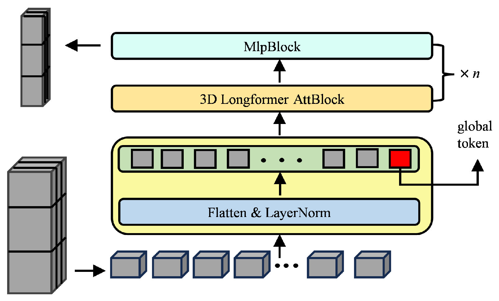
The overall structure of the MSVL is illustrated in Figure 1, which is composed of a stack of 3D Longformer structures, consisting of four stages and a final fully connected layer. As video features enter each stage, the spatial resolution decreases while the depth increases. To ensure effective extraction of temporal information from the video, temporal subsampling is applied only in the first stage, reducing the temporal dimension by a factor of 2. The subsequent stages maintain the temporal dimension unchanged. Each stage includes a complete 3D Longformer structure, consisting of three main components: the PatchEmbed, the 3D Longformer AttenBlock, and the MlpBlock, as depicted in Figure 2. In the PatchEmbed module, the input video, represented as , is divided into N patches of size in the spatial dimensions, where . Subsequently, it passes through Flatten and LayerNorm layers, and positional encoding is added, along with global tokens. PatchEmbed further reduces spatial resolution and increases depth by combining all tokens from the previous stage’s patches. The 3D Longformer AttenBlock extracts features by computing attention scores, while the MlpBlock enhances the extracted spatiotemporal features.

Figure 1.
The overall structure of MSVL. MSVL consists of 4 stages, where the spatial resolution of the video decreases, and the depth increases as the video progresses through each stage.
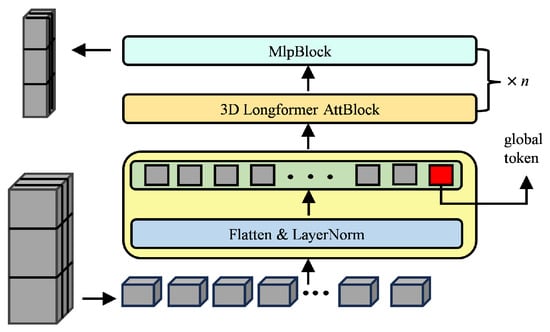
Figure 2.
Structure diagram for each stage, which is composed of three parts: PatchEmbed, 3D Longformer AttenBlock, and MlpBlock. The quantity of 3D Longformer AttenBlocks and MlpBlocks differs between stages, but each stage always begins with a PatchEmbed.
The detailed configuration parameters of the MSVL are provided in Table 1, where n represents the number of 3D Longformer AttenBlocks and MlpBlocks in each stage. refers to the spatial dimensions of the patches, is the depth of the output video features, and denote the number of attention heads and the dimension of each head, where the dimension of each head is equal to the depth of the output video features divided by the number of attention heads. specifies the number of global tokens. T, H, and W represent the dimensions of the video features, where we sample 16 frames per video, and each frame has a size of 224 × 224. defines the window size for self-attention in the spatial dimensions.

Table 1.
Network configuration parameters.
3.2. Patchembed
The PatchEmbed module consists of a Position Embedding Layer, a Flatten Layer, a Layer Normalization Layer, a Position Encoding Layer, a Dropout Layer, and a global token. It combines all tokens from the previous stage’s patches into a single token for the current stage, achieving spatial downsampling of video features while increasing their depth. The Position Embedding Layer uses Conv3D to split the input video into different patches in the spatial dimension; the video features sequentially pass through the Flatten layer and the LayerNorm layer, concatenate with positional encoding, and finally undergo Dropout before output. As videos exhibit variations in both spatial and temporal dimensions, encoding the spatial and temporal position information within the video is essential; position encoding is applied to both local tokens and global tokens as shown in Equation (1).
where represents global tokens, denotes the LayerNorm layer, E represents the position embedding layer, and represents the nth local token in the temporal dimension T.
We implement both absolute 3D position encoding and relative 3D position encoding. Absolute 3D position encoding initializes the learnable tensors using a truncated normal distribution to encode coordinates (t, x, y) in the temporal and spatial dimensions. These coordinates are concatenated and added to the input features. During training, these parameters are continuously updated, as illustrated in Equation (2).
where Cat represents the concatenation operation, and denote the x and y coordinates in the spatial dimension, and T represents the temporal dimension.
The relative 2D position encoding typically involves adding position biases during self-attention calculations, as shown in Equation (3). , , , and represent the dimensions of matrix K, and B is the positional bias.
However, this method lacks absolute spatiotemporal position information and may not be suitable for video features with both temporal and spatial dimensions. CPE [37] has proved that zero padding 3D depthwise separable convolution can overcome permutation invariance, allowing any local token at arbitrary positions to obtain its absolute spatiotemporal position by querying local tokens located at the boundary positions. In this paper, a kernel size of (3, 3, 3), a stride of (1, 1, 1), and padding of (1, 1, 1)—along with the number of groups equal to the dimensions of the current stage—are employed in 3D depthwise separable convolution to calculate the 3D relative positional encoding of local tokens, as shown in Equation (4).
where represents 3D depthwise separable convolution, and the global token utilizes absolute positional encoding initialized with truncated normal distribution.
3.3. 3D Longformer Attenblock and Mlpblock
The 3D Longformer AttenBlock consists of a Layer Normalization Layer, 3D Longformer Attention, and a Dropout Layer. Input video features undergo Layer Normalization and then pass through a multi-head self-attention layer (MSA) comprising the 3D Longformer Attention. The output of MSA is combined with the input features through residual connections and Dropout, as shown in Equation (5).
The 3D Longformer Attention, characterized by convolution-like sparse computations, effectively reduces local redundancy and decreases computational complexity while maintaining global modeling capabilities. To elaborate, an equivalent number of global tokens is introduced, corresponding to the temporal dimension T. These global tokens enable attention calculations involving all local tokens within the input video features, facilitating global modeling and communication among distant local tokens via the global tokens. Local tokens are allowed to perform attention calculations with both global tokens and local tokens within a spatial window. Since actions demonstrate temporal coherence across video frames, we enable attention calculations for local and global tokens at different frames, as illustrated in Figure 3.
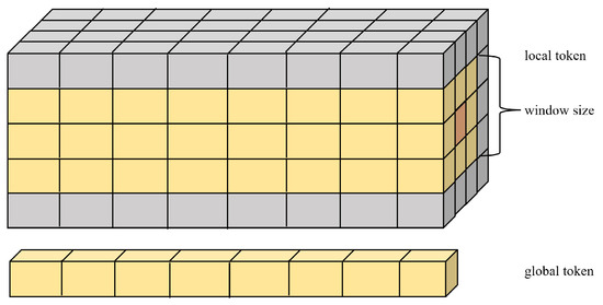
Figure 3.
Diagram of the 3D Longformer Attention mechanism. We add the same number of global tokens as the temporal dimension T in attention calculations; local tokens only perform attention calculations within the window size in spatial dimension.
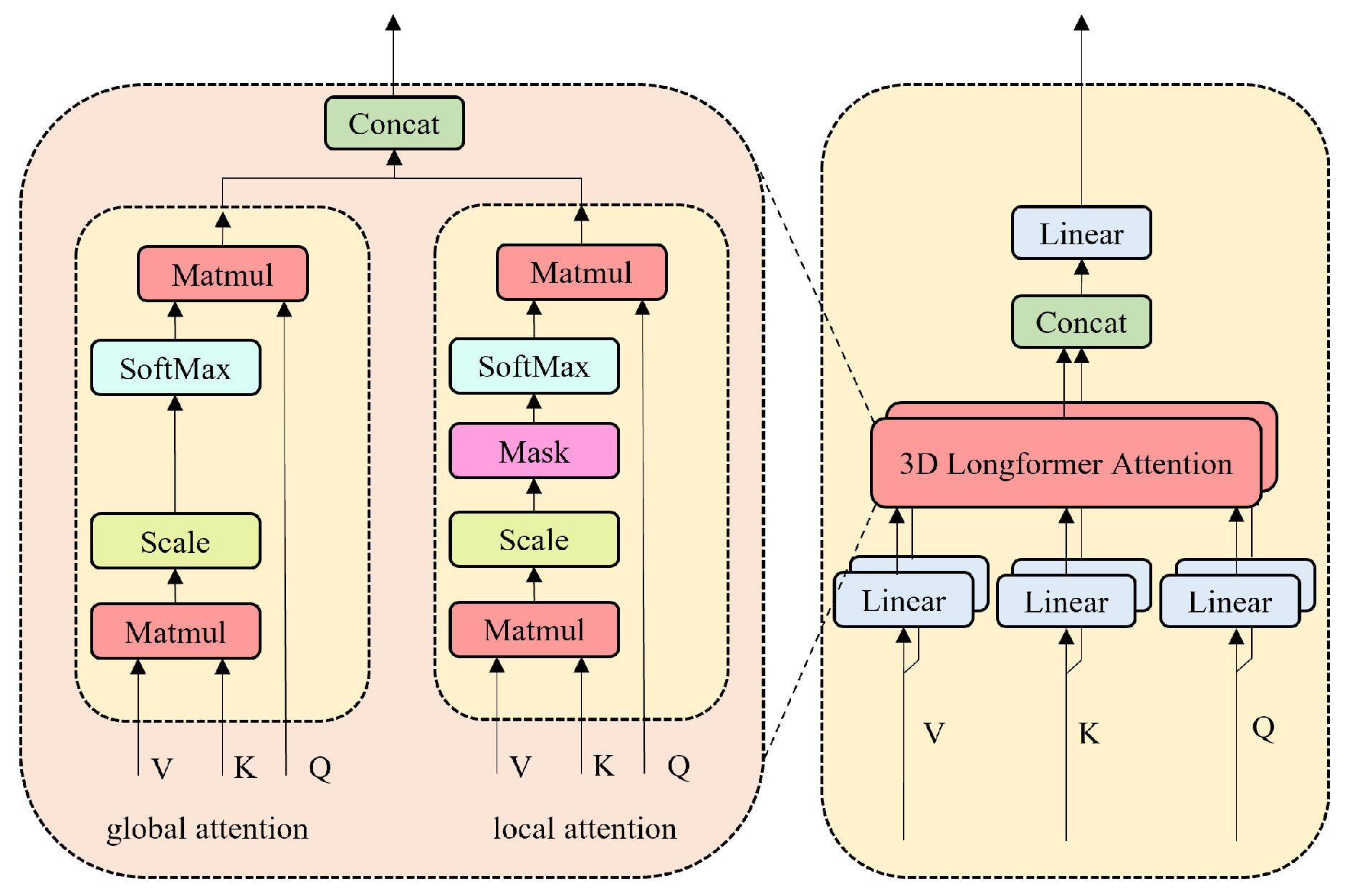
In 3D Longformer Attention, Q, K, and V are divided into global attention and local attention branches, corresponding to the attention calculation for global tokens and local tokens, respectively. In the global attention branch, standard multi-head attention calculations are performed. In the local attention branch, tokens outside a specified window size are masked, allowing only tokens within the window size to participate in attention calculations. The results from both the global and local branches are concatenated, as illustrated in Figure 4. By setting the window size to 15 × 15, the 3D Longformer Attention selectively employs a convolution-like sparse computation mechanism for local window attention calculations in stage1 (: 56 × 56) and stage2 (: 28 × 28), reducing local redundancy and extracting features. In stage3 (: 14 × 14) and stage4 (: 7 × 7), the local window attention transforms into a dense computation mechanism akin to transformers to enhance performance.

Figure 4.
Diagram of the 3D Longformer Attention structure.
The MlpBlock consists of a Layer Normalization Layer, an Mlp Layer, and a Dropout Layer. Video features outputted from the 3D Longformer AttenBlock undergo Layer Normalization, Mlp processing, and are then combined with the input through residual connections. Finally, a Dropout layer is applied before output, as shown in Equation (6).
4. Experiments
In this section, we validate the effectiveness of our method through experiments conducted on multiple datasets. Firstly, in Section 4.1, we provide a detailed description of the datasets we used. In Section 4.2, we introduce the hardware and software environment for these experiments. Subsequently, in Section 4.3, we conduct ablation experiments to explore the optimal combination of our method and use this combination to train MSVL on our assembly action dataset. In Section 4.4, we compare our method with state-of-the-art approaches. Finally, in Section 4.5, we visualize the network and present cases where the network predictions were incorrect.
4.1. Dataset
4.1.1. Assembly Action Dataset
Unlike typical human action datasets, the assembly action dataset primarily encompasses upper-body operations. These actions often involve the use of specific assembly tools and exhibit high repeatability with significant similarities among different actions. Since there is currently no publicly available standard dataset for assembly action recognition in the industrial domain, we established an assembly action dataset consisting of eight different assembly actions, including snipping, cutting, grinding, hammering, brushing, wrapping, turning screws, and turning wrenches, as shown in Figure 5. The dataset was captured using an Intel RealSense D435i camera, manufactured by Intel Corporation, Santa Clara, CA, USA, at a frame rate of 30 frames per second and a resolution of 640 × 480. Each action was recorded in 100 video segments, with each segment lasting for 5 s, resulting in a total of 800 video segments. These segments were organized into corresponding folders based on action categories. The dataset was further split into a training set (90%) and a test set (10%), with 20% of the training set reserved for validation purposes.
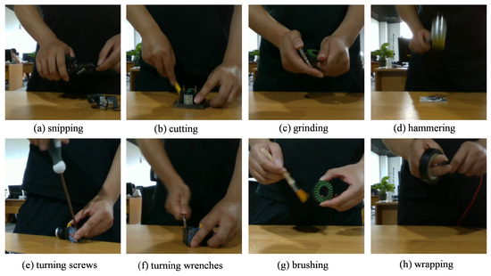
Figure 5.
Assembly action dataset.
4.1.2. Ucf101 Dataset
UCF101 [38] was created by a research team from the University of Central Florida (UCF) and is composed of 13,320 video clips downloaded from YouTube, with approximately 70% serving as the training set and about 30% as the validation set. It covers a total of 101 action categories distributed across 5 major action types. UCF101 boasts approximately 27 h of video content, and each action category typically includes between 100 and 800 video examples.
4.1.3. Hmdb51 Dataset
HMDB51 [39] was released by Brown University. This dataset primarily comprises video clips extracted from movies, alongside some clips obtained from public databases and online video platforms such as YouTube. HMDB51 consists of 6766 video clips spanning 51 action categories with approximately 70% serving as the training set and about 30% as the validation set. The dataset collectively offers around 7 h of video content, with each action category containing at least 101 examples.
4.2. Experimental Environment
The experiment was conducted under the following conditions: Intel(R) Xeon(R) Gold 6248R CPU, 128 GB memory, NVIDIA RTX 3090 GPU, Windows 10 operating system, PyTorch 1.10.2, CUDA 11.4, and Python 3.8.12. The training configuration includes a batch size of 4, running for 100 epochs and utilizing the AdamW optimizer. The chosen loss function is SoftTargetCrossEntropy, the learning rate is updated using the CosineAnnealingLR strategy with WarmUp, the initial learning rate is set to 1 × , and the minimum learning rate is set to 1 × . The video is sampled with 16 frames at a sampling rate of 4. MixUp data augmentation is applied with an alpha value of 0.8, and label smoothing is set to 0.1. The image cropping size used for both training and testing is 224 × 224 pixels. During training, we follow the approach used in the SlowFast repository [40], where videos are randomly cropped for validation. For testing, we set the number of crops to 1 and the number of views to 4.
4.3. Evaluation Metrics
In the experiment, we utilized top-1 and top-5 accuracy as the evaluation metrics for accuracy. top-1 accuracy involves comparing the predicted class with the highest confidence score to the true class label for each sample. If the top prediction aligns with the true label, it is considered a correct classification (Equation (7)).
where represents the number of correct predictions, and T represents the total number of samples.
On the contrary, top-5 accuracy takes a more lenient approach by evaluating whether the correct label is among the top five predictions. This is determined by examining the predicted classes with the top five highest confidence scores (Equation (8)).
where represents the number of samples where the correct class is in the top five predictions.
4.4. Hyperparameter Tuning
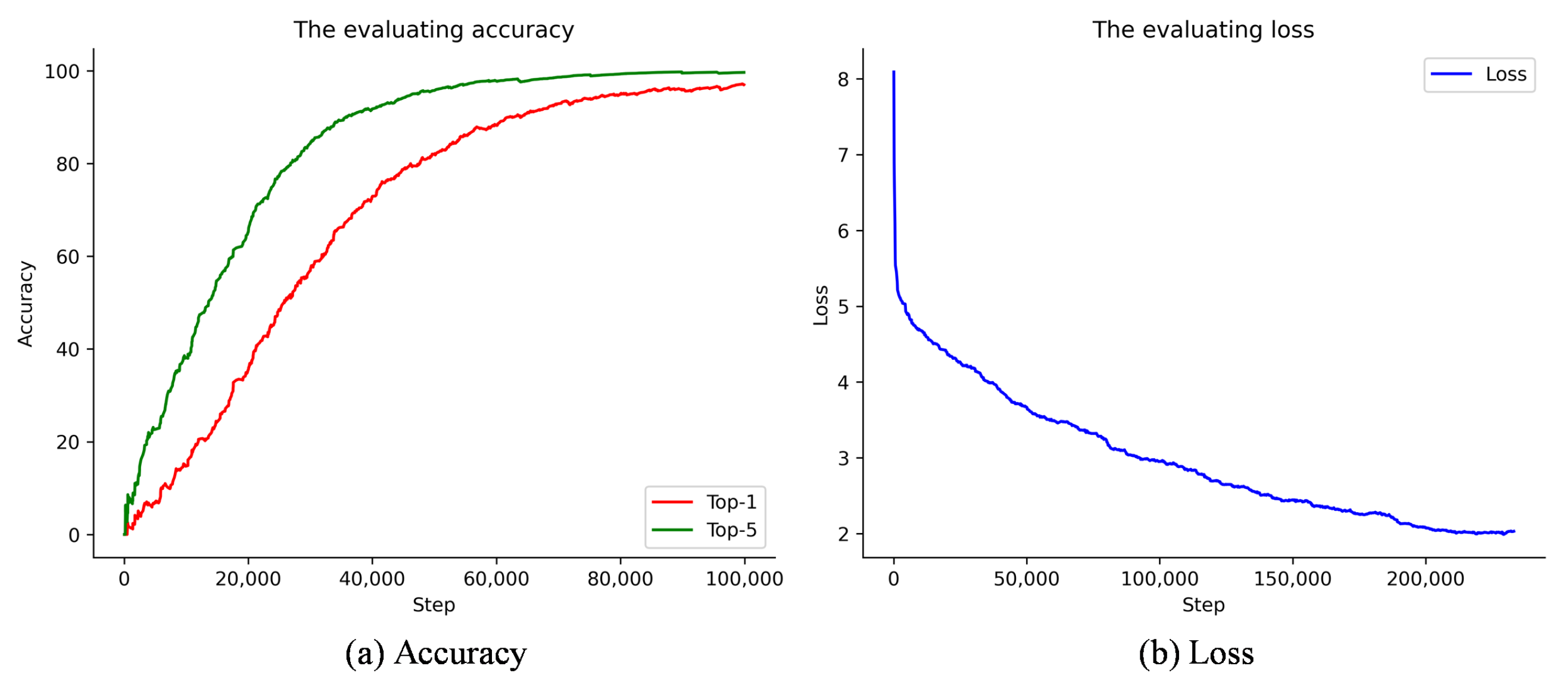
We utilized the pretrained ViL weights on ImageNet-1K, provided by EsViT repository [41] as the initial weights. We extended them to accommodate the temporal dimension for video tasks through inflation. Since training MSVL on the HMDB51 dataset leads to severe overfitting issues, resulting in poor accuracy, we first trained MSVL on the larger UCF101 dataset for 100 epochs with a warm-up of 10 epochs. Our MSVL achieved a top-1 accuracy of 97.6% on the UCF101 dataset. In Figure 6, we have plotted the top-1 accuracy, top-5 accuracy, and loss curves on the validation set.
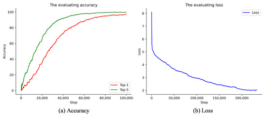
Figure 6.
Training results of MSVL on the UCF101 dataset.
Table 2 presents the prediction accuracy of MSVL across various categories in the UCF101 dataset. While the accuracy for most categories reached 100%, the category with the lowest accuracy is “WalkingWithDog”, standing at only 80.62%. Upon reviewing the confusion matrix of MSVL on the UCF101 dataset (Appendix A), we identified that 12 samples categorized as “WalkingWithDog” were inaccurately identified as “HorseRiding”. This directly contributes to the low accuracy observed in the “WalkingWithDog” category. Firstly, this misstep can be attributed to the limited samples in the “WalkingWithDog” category, as there are only 123 video files in this category in the UCF101 dataset, fewer than the average number of videos per category, which is 130.59. This limitation hinders MSVL’s capacity to learn sufficient features for precise recognition. Secondly, appearance features appear to dominate over motion characteristics in distinguishing between “WalkingWithDog” and “HorseRiding”. Since MSVL is sensitive to actions and does not prioritize the extraction of target features; while these two categories share similar actions in some samples, this could lead to confusion in MSVL due to the similarity in motion features.

Table 2.
Accuracy for different categories in the UCF101 dataset.
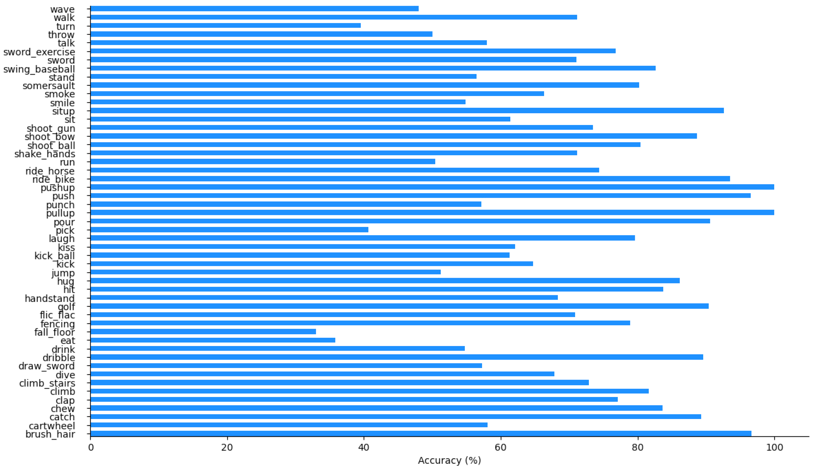
We utilized weights pretrained on the UCF101 dataset to train MSVL on the HMDB51 dataset. The training process spanned 100 epochs, with an initial warm-up period of 10 epochs, and the learning rate was set to 1 . Consequently, MSVL achieved a top-1 accuracy of 72.94% on the HMDB51 dataset and the distribution of accuracies across different categories is presented in Figure 7. It can be observed that, although a relatively high overall accuracy is achieved, there are still some actions that are prone to confusion. For example, it sometimes classifies “walk“ as “run”, or “stand“ as “jump”. One reason is that actions with a smaller field-of-view tend to receive less attention, causing MSVL to focus more on irrelevant information. Another factor is that the HMDB51 dataset consists of clips extracted from movies and, in some clips, background actors perform different actions from the main actors, introducing significant background interference.
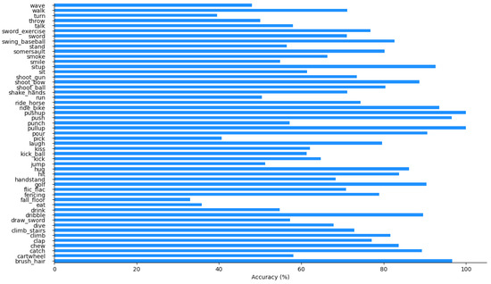
Figure 7.
The accuracy for each category in the HMDB51 dataset.
To explore the effectiveness of the 3D Longformer and the optimal configuration for MSVL, we conducted hyperparameter tuning on MSVL with different parameters and network configurations using the HMDB51 dataset. Firstly, we investigated the impact of different positional encodings. Then, we tested the use of different numbers of 3D Longformer Attention Blocks and MlpBlocks. Finally, we investigated the role of global tokens in network feature extraction by determining whether they were passed to the next stage. We present the accuracy and loss of MSVL with four distinct network configurations in Figure 8. In the legend, “Rpe“ denotes relative 3D position encoding, “Ape” denotes absolute 3D position encoding, “1191” signifies the specific network architecture employed, and “Glo” indicates the practice of passing global tokens to the next stage.

Figure 8.
The accuracy and loss of MSVL with four different network configurations on the HMDB51 dataset, employing the same training strategy.
4.4.1. Position Encoding
We tested two encoding methods of MSVL, absolute 3D position encoding (Ape), and relative 3D position encoding (Rpe). The results for top-1 and top-5 accuracies, FLOPs, and parameters on the HMDB51 dataset are presented in Table 3. Remarkably, the utilization of absolute 3D position encoding resulted in a reduction of 1G FLOPs compared to relative 3D position encoding, while maintaining consistent parameters. However, relative 3D position encoding also notably improved top-1 accuracy by 2.76% and top-5 accuracy by 1.97%.

Table 3.
Ablations on different position encoding of MSVL on the HMDB51 dataset.
To investigate the reasons behind the superior performance of relative 3D position encoding over absolute 3D position encoding, we visualized the position encoding of four stages in both scenarios, as depicted in Figure 9. Our observations revealed that relative 3D position encoding, which relies on 3D depthwise separable convolution, can capture spatiotemporal positional information from local tokens, simultaneously enhancing the features. On the contrary, the absolute 3D position encoding contains no feature information and solely provides positional information. We think this disparity leads to the superior generalization performance of relative 3D position encoding compared to absolute 3D position encoding.
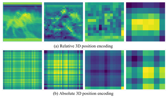
Figure 9.
Visualization of absolute 3D position encoding and relative 3D position encoding.
4.4.2. Number of 3D Longformer Attenblocks and Mlpblocks
We investigated the impact of different numbers (n) of 3D Longformer AttenBlock and MlpBlock layers in each stage. To ensure a fair experiment, we set the total count of n to be equal. To be specific, we employed two network structures—(1, 1, 9, 1), resembling a transformer hierarchy, and (1, 2, 8, 1), resembling a convolutional network hierarchy—both using relative 3D position encoding. As shown in Table 4, the (1, 1, 9, 1) structure reduced FLOPs by 2G but increased Params by 1.2M compared to (1, 2, 8, 1). Furthermore, the (1, 1, 9, 1) structure lagged behind (1, 2, 8, 1) by 1.97% in top-1 accuracy and 0.97% in top-5 accuracy.

Table 4.
Ablations about how many 3D Longformer AttenBlocks and MlpBlocks to insert.
From the data presented above, it is evident that the (1, 2, 8, 1) structure, which resembles a convolutional network hierarchy, is better suited for MSVL. We believe this is related to the feature extraction process and network architecture of MSVL. MSVL employs high resolution feature maps for extracting local information in shallow layers and low resolution feature maps for capturing global information in deeper layers, all while progressively increasing the feature depth, which aligns more closely with the characteristics of convolutional neural networks.
4.4.3. Passing Global Tokens to the Next Stage
In each stage, global tokens generate global features by attending to all local tokens. However, in the standard ViL structure, only input features were passed to the next stage, and old global tokens were discarded, with new global tokens initialized in the patch embedding. We conducted experiments to evaluate the impact of sequentially passing global tokens to the next stage. To ensure the smooth transfer of global tokens from the previous stage to the next stage, we trimmed a portion of the global tokens’ data during the transfer process to match the dimensions of the next stage. The comparative results are presented in Table 5. It was observed that passing global tokens to the next stage had no impact on FLOPs and Params but improved top-1 accuracy by 1.56% and top-5 accuracy by 0.5%. Furthermore, we noticed that the practice of passing global tokens leads to faster network convergence during the early stages of training (within the first 20,000 steps), as shown in Figure 8.

Table 5.
Ablations about whether to pass global tokens to the next stage.
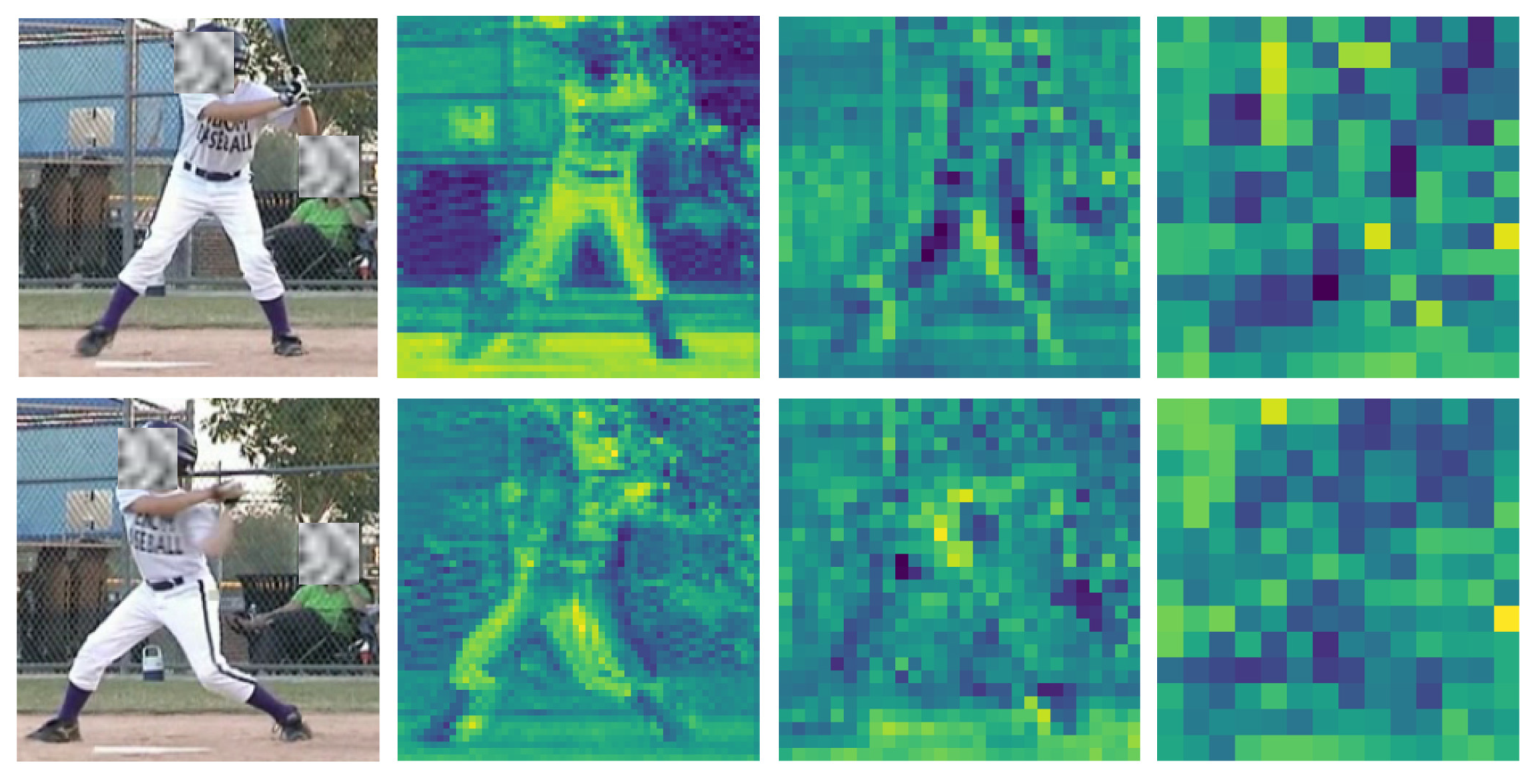
We believe that one significant reason for the improvement in accuracy is that these global tokens contain global features, which represent essential spatiotemporal features of the video and allow local tokens to better understand the video context. In Figure 10, we visualize the global tokens passed at different stages. It can be observed that the global tokens passed from lower stages contain more specific spatial features, while those passed from higher stages contain more abstract features. Additionally, we also noticed the presence of shadows of human actions from the previous frame in the global tokens passed from stage 1 to stage 2. This further validates our hypothesis that global tokens capture both temporal and spatial features.

Figure 10.
For the visualization of global tokens, we selected the “swing baseball” category and displayed RGB frames, global tokens passed from stage 1 to stage 2, global tokens passed from stage 2 to stage 3, and global tokens passed from stage 3 to stage 4.
4.4.4. Training on the Assembly Action Dataset
Using ablation experiments to validate the optimal configuration, we trained MSVL on the assembly action dataset, obtaining top-1 accuracy, top-5 accuracy, and loss curves as shown in Figure 11a,b. MSVL achieved 100% top-1 and top-5 accuracy after only 4000 training steps on the assembly action dataset. Evaluating the trained MSVL on the test set, we obtained a confusion matrix for the assembly action dataset, as depicted in Figure 11c. MSVL achieved high accuracy, correctly classifying all categories.

Figure 11.
Training results of the optimal configuration of MSVL on the assembly action dataset.
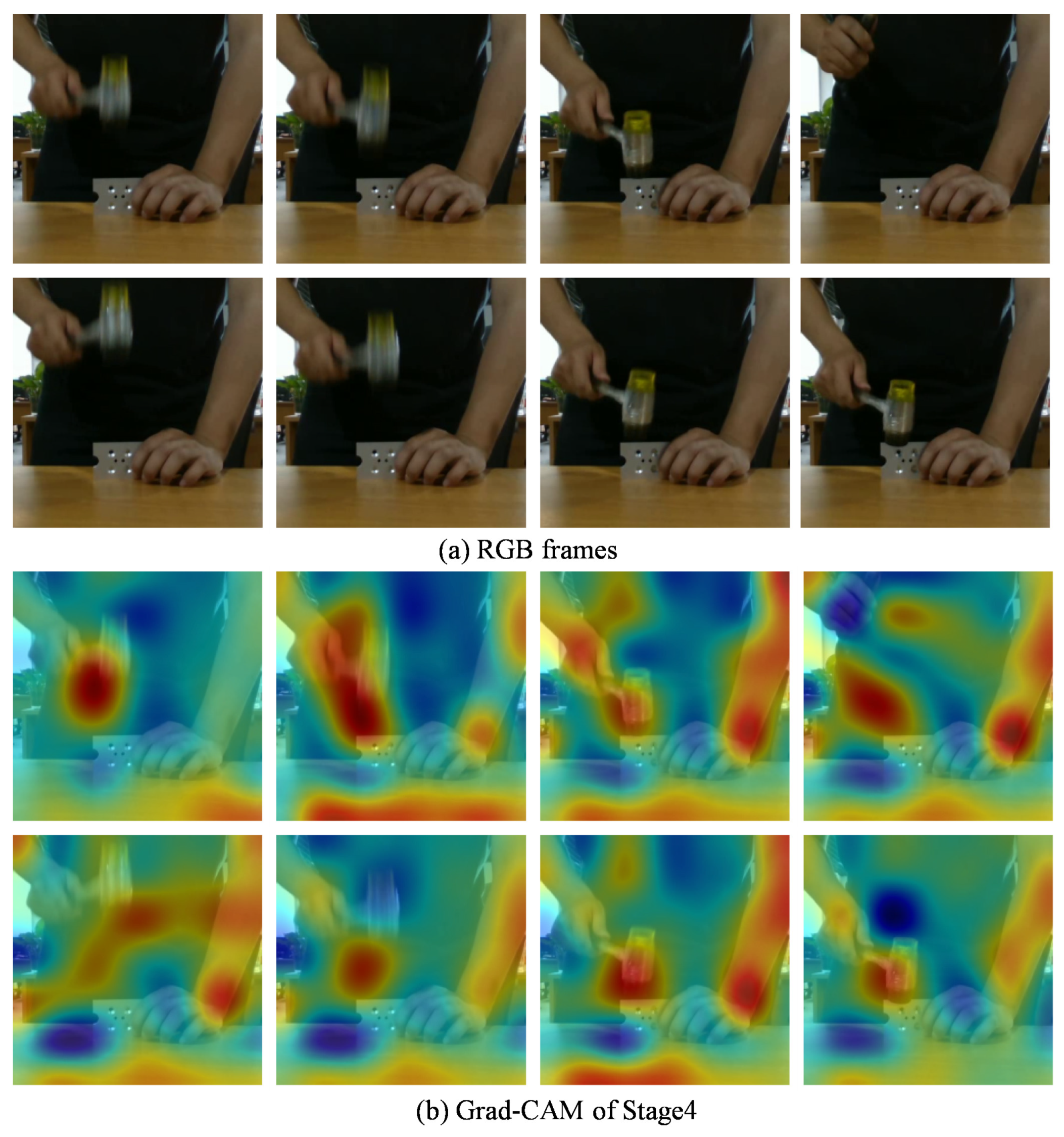
In Figure 12, we employed Grad-CAM [42] to visualize MSVL’s output in stage 4, using a video segment from the assembly action dataset demonstrating the “hammering” category. We observed that MSVL focused more attention on the hand area interacting with assembly tools and parts, differentiating the current assembly action category by assigning higher weights to these regions.

Figure 12.
We sampled 8 frames from the “hammering” action, (a) representing RGB frames and (b) displaying Grad-CAM results for stage 4.
Additionally, we visualized the feature maps of the “hammering” category produced by MSVL in each stage, as shown in Figure 13. We noticed that each patch in the feature maps had global features, which were particularly evident in stage 1 and stage 2. This indicates that global tokens played a crucial role, leveraging attention calculations between global tokens and all local tokens in the input video features, thus passing these global features to each local token, even for those located far apart.
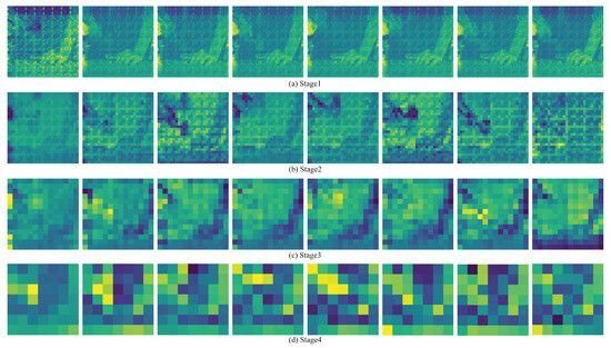
Figure 13.
Feature maps for the hammering action generated at each stage.
4.5. Comparative Experiments
We conducted comparative experiments to assess the performance of the proposed MSVL in comparison with state-of-the-art methods on the HMDB51 and UCF101 datasets. The results for top-1 and top-5 accuracies, FLOPs, and parameters are presented in Table 6. The top-1 and top-5 accuracy results, with the best, second best, and third best performances, are highlighted in red, blue, and green, respectively. All networks used only RGB frames as input with a video frame resolution of 224 × 224 pixels. For feature extraction backbones, R(2 + 1)D, TSN, I3D, and TSM employed ResNet50. divST represents the version of TimeSformer that incorporates spatiotemporal separated attention, while VideoSwin utilized the Swin-S version. We initially attempted to train TimeSformer and VideoSwin directly on the HMDB51 and UCF101 datasets but achieved suboptimal accuracy. As a result, we decided to finetune them using pretrained weights provided by mmaction2 [43]. The sampling parameters for TimeSformer are as follows: a clip length of 16, a frame interval of 2, and one clip. For VideoSwin, the parameters are 8, 32, and 1, respectively.

Table 6.
Performance comparison with the state-of-the-art on UCF-101 and HMDB-51 datasets.
In most cases, it can be observed that our MSVL achieves the best performance compared to other methods. In contrast to methods employing convolutional approaches [11,12,19,20,44], MSVL excels in extracting overall video features, demonstrating exceptional performance. In comparison to divST, MSVL harnesses 3D Longformer Attention in a joint spatiotemporal manner to extract spatiotemporal features. It also lowers computational complexity and reduces the network’s parameter count through a local attention mechanism. On the UCF-101 dataset, MSVL outperforms TimeSformer by a margin of 2.9% while simultaneously reducing the parameter count by 77.6%. VideoSwin also employs a convolution-like mechanism that recombines patches from different positions in the input video features. In comparison to VideoSwin, MSVL achieves a notable reduction in the parameter count and FLOPs by 45.1% and 4.8%, respectively. Despite not undergoing pretraining on large-scale datasets, MSVL achieves highly competitive accuracy compared to VideoSwin. We believe that, if MSVL were pretrained on similarly large-scale datasets (such as K400), its performance would further improve.
4.6. Visualization
In Figure 14, we present examples of correct and incorrect predictions by our MSVL on the HMDB51 and UCF101 datasets, and display both RGB frames and the feature maps of the four stages of MSVL. We observe that MSVL performs well on videos where the human body occupies a significant portion of the frame. However, for videos with a small proportion of the human body region, prediction errors may occur. This phenomenon could be attributed to the attention mechanism involving global and local tokens, which makes MSVL focus more on the overall global features and may neglect local characteristics. We calculated the real-time performance of the network. Our MSVL took a total of 16 min and 56 s to perform inference on 3996 videos, with each video extracting 8 frames as input to the network; this resulted in our MSVL achieving 31.45 FPS on a 3090 GPU.
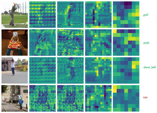
Figure 14.
Correctly predicted categories are shown in green text, while incorrectly predicted categories are shown in red text.
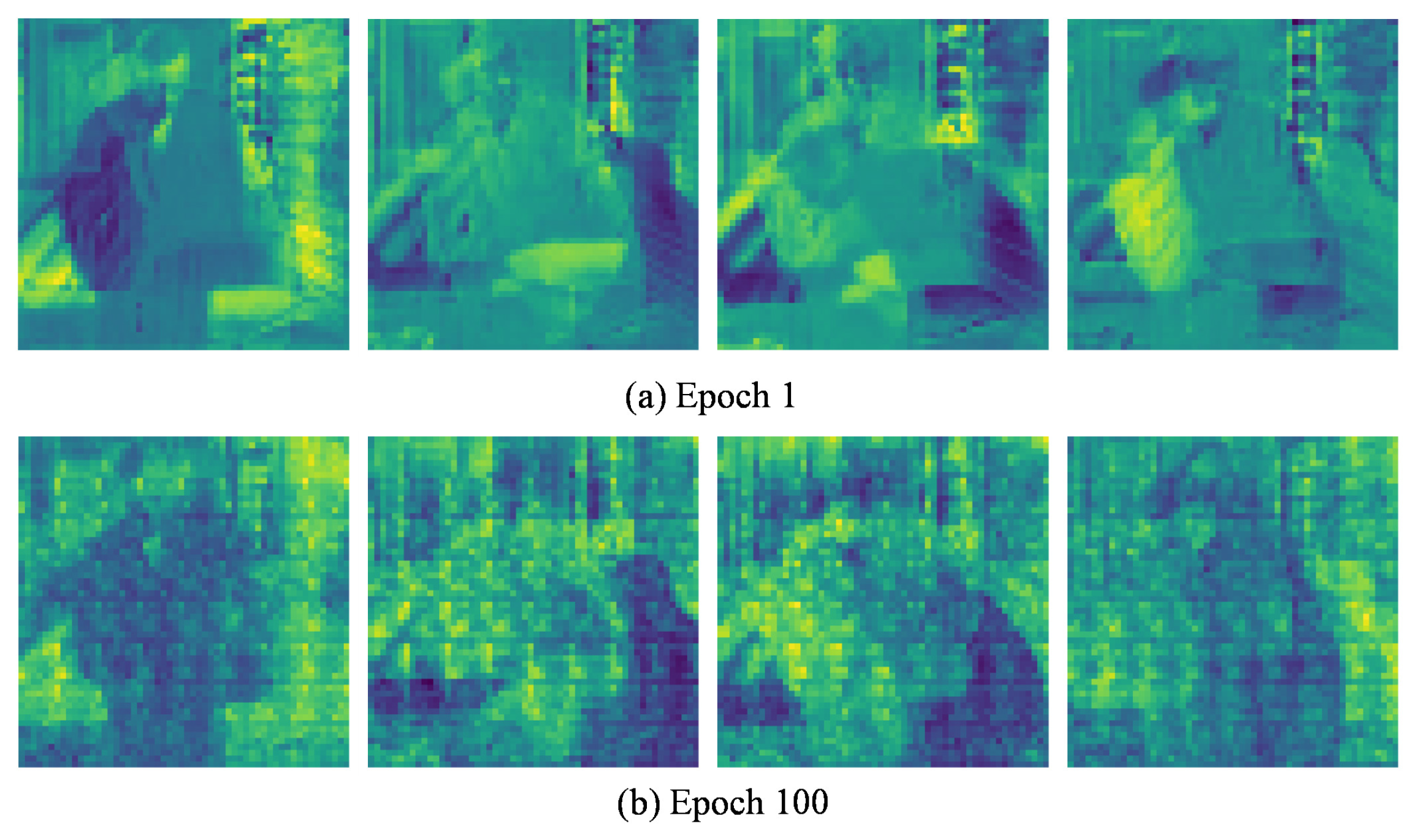
We also observed an intriguing phenomenon: the feature map patches exclusively contain global features in models trained for an extended number of epochs. In contrast, models trained for fewer epochs tend to contain predominantly local features, as illustrated in Figure 15. We posit that this phenomenon arises because global tokens only transfer these global features to each local token through attention calculations after undergoing multiple epochs of training. Furthermore, in the feature maps of the subsequent video frames, we can also observe shadows of human actions from the previous video frame, similar to those that global tokens extract. This further indicates that global tokens can pass the extracted spatiotemporal features to local tokens, thereby maintaining global features of action information from previous video frames and effectively integrating temporal and spatial features.

Figure 15.
We selected the model weights at epoch 1 and epoch 100, respectively, and generated their feature maps for the same video in stage 1 of MSVL.
5. Conclusions
This paper introduces MSVL, a Multi-Scale Video Longformer network for action recognition. MSVL effectively integrates spatiotemporal information from video sequences using the 3D Longformer structure with a “local attention + global features” attention mechanism. It reduces network computational complexity and parameter count through local window attention. Furthermore, it extracts global features via global tokens, preserving and propagating the global features of the video. Numerous ablation experiments were conducted to identify the optimal configuration for MSVL and explore the effectiveness of global tokens in video feature extraction. The architecture of MSVL is simple and achieves high accuracy on the HMDB51 and UCF101 datasets, even when using only RGB frames as input and without pretraining on large-scale datasets. Additionally, we have created an assembly action dataset comprising eight categories for assembly action recognition and achieved high accuracy using MSVL, further demonstrating its effectiveness.
Author Contributions
Methodology, C.C. and C.Z.; Software, C.Z.; Validation, C.C., C.Z. and X.D.; Visualization, C.C., C.Z. and X.D. All authors have read and agreed to the published version of the manuscript.
Funding
This research was supported in part by the Jiangsu Carbon Peak Carbon Neutrality Science and Technology Innovation Project of China under Grant BE2022044.
Institutional Review Board Statement
Not applicable.
Informed Consent Statement
Not applicable.
Data Availability Statement
Publicly available datasets were analyzed in this study. These datasets can be found here: UCF101 Dataset: https://www.crcv.ucf.edu/research/data-sets/ucf101/, accessed on 2 January 2024; HMDB51 Dataset: https://serre-lab.clps.brown.edu/resource/hmdb-a-large-human-motion-database/, accessed on 2 January 2024.
Conflicts of Interest
The authors declare no conflicts of interest.
Appendix A. The Confusion Matrix of MSVL on the UCF101 Dataset
To provide a more intuitive observation of the performance of the MSVL on the UCF101 dataset, we have visualized the confusion matrix in Figure A1. In the figure, the deeper the blue color of the diagonal elements, the higher the accuracy of the model’s prediction for that category.
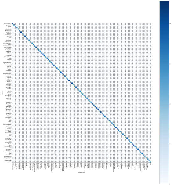
Figure A1.
Confusion matrix of MSVL on the UCF101 dataset.
Figure A1.
Confusion matrix of MSVL on the UCF101 dataset.

References
- Yang, S.; Zhao, Y.; Ma, Y. Analysis of the reasons and development of short video application-Taking Tik Tok as an example. In Proceedings of the 2019 9th International Conference on Information and Social Science (ICISS 2019), Manila, Philippines, 12–14 July 2019; pp. 12–14. [Google Scholar]
- Xiao, X.; Xu, D.; Wan, W. Overview: Video recognition from handcrafted method to deep learning method. In Proceedings of the 2016 International Conference on Audio, Language and Image Processing (ICALIP), Shanghai, China, 11–12 July 2016; pp. 646–651. [Google Scholar]
- Lavee, G.; Rivlin, E.; Rudzsky, M. Understanding video events: A survey of methods for automatic interpretation of semantic occurrences in video. IEEE Trans. Syst. Man Cybern. Part (Appl. Rev.) 2009, 39, 489–504. [Google Scholar] [CrossRef]
- Dalal, N.; Triggs, B.; Schmid, C. Human detection using oriented histograms of flow and appearance. In Proceedings of the Computer Vision–ECCV 2006: 9th European Conference on Computer Vision, Graz, Austria, 7–13 May 2006; pp. 428–441. [Google Scholar]
- Wang, H.; Schmid, C. Action recognition with improved trajectories. In Proceedings of the IEEE International Conference on Computer Vision, Sydney, Australia, 1–8 December 2013; pp. 3551–3558. [Google Scholar]
- O’Shea, K.; Nash, R. An introduction to convolutional neural networks. arXiv 2015, arXiv:1511.08458. [Google Scholar]
- Vaswani, A.; Shazeer, N.; Parmar, N.; Uszkoreit, J.; Jones, L.; Gomez, A.N.; Kaiser, Ł.; Polosukhin, I. Attention is all you need. Adv. Neural Inf. Process. Syst. 2017, 30, 6000–6010. [Google Scholar]
- Al-Berry, M.; Salem, M.M.; Hussein, A.; Tolba, M. Spatio-temporal motion detection for intelligent surveillance applications. Int. J. Comput. Methods 2015, 12, 1350097. [Google Scholar] [CrossRef]
- Simonyan, K.; Zisserman, A. Two-stream convolutional networks for action recognition in videos. Adv. Neural Inf. Process. Syst. 2014, 27, 568. [Google Scholar]
- Huang, D.A.; Ramanathan, V.; Mahajan, D.; Torresani, L.; Paluri, M.; Fei-Fei, L.; Niebles, J.C. What makes a video a video: Analyzing temporal information in video understanding models and datasets. In Proceedings of the IEEE Conference on Computer Vision and Pattern Recognition, Salt Lake City, UT, USA, 18–23 June 2018; pp. 7366–7375. [Google Scholar]
- Tran, D.; Bourdev, L.; Fergus, R.; Torresani, L.; Paluri, M. Learning spatiotemporal features with 3d convolutional networks. In Proceedings of the IEEE International Conference on Computer Vision, Santiago, Chile, 7–13 December 2015; pp. 4489–4497. [Google Scholar]
- Carreira, J.; Zisserman, A. Quo vadis, action recognition? A new model and the kinetics dataset. In Proceedings of the IEEE Conference on Computer Vision and Pattern Recognition, Honolulu, HI, USA, 21–26 July 2017; pp. 6299–6308. [Google Scholar]
- Albawi, S.; Mohammed, T.A.; Al-Zawi, S. Understanding of a convolutional neural network. In Proceedings of the 2017 International Conference on Engineering and Technology (ICET), Antalya, Turkey, 21–23 August 2017; pp. 1–6. [Google Scholar]
- Li, Z.; Liu, F.; Yang, W.; Peng, S.; Zhou, J. A survey of convolutional neural networks: Analysis, applications, and prospects. IEEE Trans. Neural Networks Learn. Syst. 2021, 33, 6999–7019. [Google Scholar] [CrossRef] [PubMed]
- Dosovitskiy, A.; Beyer, L.; Kolesnikov, A.; Weissenborn, D.; Zhai, X.; Unterthiner, T.; Dehghani, M.; Minderer, M.; Heigold, G.; Gelly, S.; et al. An image is worth 16x16 words: Transformers for image recognition at scale. arXiv 2020, arXiv:2010.11929. [Google Scholar]
- Bertasius, G.; Wang, H.; Torresani, L. Is space-time attention all you need for video understanding? In Proceedings of the 2021 International Conference on Machine Learning, Online, 18–24 July 2021; Volume 2, p. 4. [Google Scholar]
- Fan, H.; Xiong, B.; Mangalam, K.; Li, Y.; Yan, Z.; Malik, J.; Feichtenhofer, C. Multiscale vision transformers. In Proceedings of the IEEE/CVF International Conference on Computer Vision, Montreal, BC, Canada, 11–17 October 2021; pp. 6824–6835. [Google Scholar]
- Beltagy, I.; Peters, M.E.; Cohan, A. Longformer: The long-document transformer. arXiv 2020, arXiv:2004.05150. [Google Scholar]
- Wang, L.; Xiong, Y.; Wang, Z.; Qiao, Y.; Lin, D.; Tang, X.; Van Gool, L. Temporal segment networks: Towards good practices for deep action recognition. In Proceedings of the European Conference on Computer Vision, Amsterdam, The Netherlands, 11–14 October 2016; Springer: Berlin/Heidelberg, Germany, 2016; pp. 20–36. [Google Scholar]
- Tran, D.; Wang, H.; Torresani, L.; Ray, J.; LeCun, Y.; Paluri, M. A closer look at spatiotemporal convolutions for action recognition. In Proceedings of the IEEE Conference on Computer Vision and Pattern Recognition, Salt Lake City, UT, USA, 18–23 June 2018; pp. 6450–6459. [Google Scholar]
- Sun, C.; Shrivastava, A.; Vondrick, C.; Murphy, K.; Sukthankar, R.; Schmid, C. Actor-centric relation network. In Proceedings of the European Conference on Computer Vision (ECCV), Munich, Germany, 8–14 September 2018; pp. 318–334. [Google Scholar]
- Wu, C.Y.; Feichtenhofer, C.; Fan, H.; He, K.; Krahenbuhl, P.; Girshick, R. Long-term feature banks for detailed video understanding. In Proceedings of the IEEE/CVF Conference on Computer Vision and Pattern Recognition, Long Beach, CA, USA, 15–20 June 2019; pp. 284–293. [Google Scholar]
- Feichtenhofer, C.; Fan, H.; Malik, J.; He, K. Slowfast networks for video recognition. In Proceedings of the IEEE/CVF International Conference on Computer Vision, Seoul, Republic of Korea, 27 October–2 November 2019; pp. 6202–6211. [Google Scholar]
- Wang, X.; Girshick, R.; Gupta, A.; He, K. Non-local neural networks. In Proceedings of the IEEE Conference on Computer Vision and Pattern Recognition, Salt Lake City, UT, USA, 18–23 June 2018; pp. 7794–7803. [Google Scholar]
- Girdhar, R.; Carreira, J.; Doersch, C.; Zisserman, A. Video action transformer network. In Proceedings of the IEEE/CVF Conference on Computer Vision and Pattern Recognition, Long Beach, CA, USA, 15–20 June 2019; pp. 244–253. [Google Scholar]
- Arnab, A.; Dehghani, M.; Heigold, G.; Sun, C.; Lučić, M.; Schmid, C. Vivit: A video vision transformer. In Proceedings of the IEEE/CVF International Conference on Computer Vision, Montreal, BC, Canada, 11–17 October 2021; pp. 6836–6846. [Google Scholar]
- Zhang, Y.; Li, X.; Liu, C.; Shuai, B.; Zhu, Y.; Brattoli, B.; Chen, H.; Marsic, I.; Tighe, J. Vidtr: Video transformer without convolutions. In Proceedings of the IEEE/CVF International Conference on Computer Vision, Montreal, BC, Canada, 11–17 October 2021; pp. 13577–13587. [Google Scholar]
- Liu, X.; Wang, Q.; Hu, Y.; Tang, X.; Zhang, S.; Bai, S.; Bai, X. End-to-end temporal action detection with transformer. IEEE Trans. Image Process. 2022, 31, 5427–5441. [Google Scholar] [CrossRef] [PubMed]
- Weng, Y.; Pan, Z.; Han, M.; Chang, X.; Zhuang, B. An Efficient Spatio-Temporal Pyramid Transformer for Action Detection. In Proceedings of the European Conference on Computer Vision, Tel Aviv, Israel, 23–27 October 2022; Avidan, S., Brostow, G., Cissé, M., Farinella, G.M., Hassner, T., Eds.; Springer Nature: Cham, Switzerland, 2022; pp. 358–375. [Google Scholar]
- Wu, C.Y.; Li, Y.; Mangalam, K.; Fan, H.; Xiong, B.; Malik, J.; Feichtenhofer, C. Memvit: Memory-augmented multiscale vision transformer for efficient long-term video recognition. In Proceedings of the IEEE/CVF Conference on Computer Vision and Pattern Recognition, New Orleans, LA, USA, 18–24 June 2022; pp. 13587–13597. [Google Scholar]
- Wei, C.; Fan, H.; Xie, S.; Wu, C.Y.; Yuille, A.; Feichtenhofer, C. Masked feature prediction for self-supervised visual pre-training. In Proceedings of the IEEE/CVF Conference on Computer Vision and Pattern Recognition, New Orleans, LA, USA, 18–24 June 2022; pp. 14668–14678. [Google Scholar]
- Tong, Z.; Song, Y.; Wang, J.; Wang, L. Videomae: Masked autoencoders are data-efficient learners for self-supervised video pre-training. Adv. Neural Inf. Process. Syst. 2022, 35, 10078–10093. [Google Scholar]
- Liu, Z.; Ning, J.; Cao, Y.; Wei, Y.; Zhang, Z.; Lin, S.; Hu, H. Video swin transformer. In Proceedings of the IEEE/CVF Conference on Computer Vision and Pattern Recognition, New Orleans, LA, USA, 18–24 June 2022; pp. 3202–3211. [Google Scholar]
- Li, K.; Wang, Y.; Gao, P.; Song, G.; Liu, Y.; Li, H.; Qiao, Y. Uniformer: Unified transformer for efficient spatiotemporal representation learning. arXiv 2022, arXiv:2201.04676. [Google Scholar]
- Neimark, D.; Bar, O.; Zohar, M.; Asselmann, D. Video transformer network. In Proceedings of the IEEE/CVF International Conference on Computer Vision, Montreal, BC, Canada, 11–17 October 2021; pp. 3163–3172. [Google Scholar]
- Zhang, P.; Dai, X.; Yang, J.; Xiao, B.; Yuan, L.; Zhang, L.; Gao, J. Multi-scale vision longformer: A new vision transformer for high-resolution image encoding. In Proceedings of the IEEE/CVF International Conference on Computer Vision, Montreal, BC, Canada, 11–17 October 2021; pp. 2998–3008. [Google Scholar]
- Chu, X.; Zhang, B.; Tian, Z.; Wei, X.; Xia, H. Do we really need explicit position encodings for vision transformers. arXiv 2021, arXiv:2102.10882. [Google Scholar]
- Soomro, K.; Zamir, A.R.; Shah, M. UCF101: A dataset of 101 human actions classes from videos in the wild. arXiv 2012, arXiv:1212.0402. [Google Scholar]
- Kuehne, H.; Jhuang, H.; Garrote, E.; Poggio, T.; Serre, T. HMDB: A large video database for human motion recognition. In Proceedings of the 2011 International Conference on Computer Vision, Washington, DC, USA, 6–13 November 2011; pp. 2556–2563. [Google Scholar]
- Fan, H.; Li, Y.; Xiong, B.; Lo, W.Y.; Feichtenhofer, C. PySlowFast. 2020. Available online: https://github.com/facebookresearch/slowfast (accessed on 23 January 2024).
- Li, C.; Yang, J.; Zhang, P.; Gao, M.; Xiao, B.; Dai, X.; Yuan, L.; Gao, J. Efficient self-supervised vision transformers for representation learning. arXiv 2021, arXiv:2106.09785. [Google Scholar]
- Selvaraju, R.R.; Cogswell, M.; Das, A.; Vedantam, R.; Parikh, D.; Batra, D. Grad-cam: Visual explanations from deep networks via gradient-based localization. In Proceedings of the IEEE International Conference on Computer Vision, Venice, Italy, 22–29 October 2017; pp. 618–626. [Google Scholar]
- Contributors, M. OpenMMLab’s Next Generation Video Understanding Toolbox and Benchmark. 2020. Available online: https://github.com/open-mmlab/mmaction2 (accessed on 23 January 2024).
- Lin, J.; Gan, C.; Han, S. TSM: Temporal Shift Module for Efficient Video Understanding. In Proceedings of the IEEE International Conference on Computer Vision, Seoul, Republic of Korea, 27 October–2 November 2019. [Google Scholar]
Disclaimer/Publisher’s Note: The statements, opinions and data contained in all publications are solely those of the individual author(s) and contributor(s) and not of MDPI and/or the editor(s). MDPI and/or the editor(s) disclaim responsibility for any injury to people or property resulting from any ideas, methods, instructions or products referred to in the content. |
© 2024 by the authors. Licensee MDPI, Basel, Switzerland. This article is an open access article distributed under the terms and conditions of the Creative Commons Attribution (CC BY) license (https://creativecommons.org/licenses/by/4.0/).


