Article

A New Framework for Active Loss Reduction and Voltage Profile Enhancement in a Distributed Generation-Dominated Radial Distribution Network

1
Department of Electrical Engineering, French South African Institute of Technology (F’SATI), Tshwane University of Technology, Pretoria 0001, South Africa
2
École Supérieure d’Ingénieurs en Électrotechnique et Électronique, Cité Descarte Boulevard Blaise Pascal, Noisy-le-Grand, 93160 Paris, France
*
Author to whom correspondence should be addressed.
Appl. Sci. 2024, 14(3), 1077; https://doi.org/10.3390/app14031077
Submission received: 20 November 2023 / Revised: 15 January 2024 / Accepted: 22 January 2024 / Published: 26 January 2024
(This article belongs to the Special Issue Power Systems Stability in Current and Future Scenarios)

Abstract

:
In recent times, a significant amount of power loss and system instability due to high voltage deviation experienced by modern power systems, in addition to the pressing issues challenging the power industry such as pollution—especially the emission of greenhouse gases—and aging infrastructures, have posed a serious threat to system operations. Distributed generation has been identified as one main solution capable of reducing pollution when solar and wind power are used and, hence, rejuvenating dilapidated infrastructures and redeeming climatic changes. This paper presents a novel two-stage approach for the identification of suitable locations for DG placement and the sizing of DG for loss reduction and voltage stability enhancement. The first stage explored the use of a network structure to develop a coupling factor (CF) approach that was non-iterative in nature to determine suitable DG locations. In the second stage, the size of the DG was determined using the particle swarm optimization (PSO) algorithm. The main objective was to obtain an optimal voltage profile of the system under consideration while lowering the power loss in the system and ensuring network stability amidst DG incorporation. The model design, optimization and simulation were carried out using the MATLAB 2016a environment and the IEEE 33-bus test system, in which DG was integrated. The influence of increasing the level of DG placement in the system was then investigated. The forward/backward sweep method was applied to monitor the optimization process. The voltage profiles for both the base case when no DG was integrated and the case of incremental DG integration were considered. The results obtained for both single and multiple DG integration are compared with those obtained using the existing methods. The results show the efficiency and applicability of the new non-iterative scheme in the quick identification of DG locations for voltage profile enhancement and network real power loss reduction in radial distribution networks.

1. Introduction

Energy supply deficiency and climate change have resulted in the rapid growth of distributed generation technology [1]. This growth can also be attributed to the cleaner renewable sources that constitute most DGs and aging equipment [2,3]. Distributed generation has numerous definitions and names like dispersed generation, embedded generation and decentralized generation. But, among all these terms, distributed generation is the most common [4,5]. Distributed generation, irrespective of its advantages, can cause instability in voltage and other power practices like the power factor, reactive power and frequency when interconnected to an existing grid [6,7,8]. The instability problem can occur as a result of the intermittency of renewable sources, non-radial power flow, over-voltage and management [9]. Most of the practical distribution power networks have been designed to operate on a one-directional power flow feeder, most commonly known as a radial system [10,11,12]. With these radial systems, protection schemes have become rather standard and also straightforward, and this is based on common phase and neutral/ground non-directional overcurrent protection [2].
However, the addition of DG to existing radial systems would change this basic protective system in terms of design and structure to accommodate the integration of DGs in these systems. Consequently, challenges including keeping required voltage levels within preferred limits are bound to manifest [7,13]. That is why a careful and analytical investigation needs to be performed on all power and protective systems before DG integration to avoid the complete breakdown of these entire systems [13]. It is for this reason that a maximum allowable penetration is recommended at every interconnection point of DG [14]. Apart from the voltage stability problem, there exists an angle stability problem and a frequency stability problem, but both the angle problem and the frequency problem are not often seen in distribution systems [15]. A grid-tied or micro-grid system can be referred to as autonomous, and its mode of interconnection may be based on an inverter system for solar PV and energy storage devices or a synchronous or induction motor system for wind generation and standard fossil fuel-based motor generators [4].
There are other factors that affect voltages in distribution systems besides the connecting generator in the distribution system. Ordinarily, without DG, the distance of the transmission or the length of the cable brings about variation in voltage profiles [12]. When a DG is connected, the location of the DG, DG output or capacity, DG dispersion, the feeder’s conductor, the load profile and the primary voltage setting are the factors that can equally vary the voltage profile of the distribution system [16,17]. Increasing DG output could either be increasing the real power or the reactive power but in most cases the active power [18,19] midst the other factors, location of DG which is the distance from the substation to the customer point is an important consideration in the study of voltage stability due to voltage drop [20]. Voltage will rise due to DG integration and this rise is directly proportional to the distance (linear) with the distance along the line to the point of DG connection [21].
In recent times, under-voltage has been one of the major areas in the active stream of research on radial distribution systems that are dominated by distributed generators. The increasing load on existing power system infrastructure has continued to stretch the nominal voltage [4]. The growth in the population and the advent of technology have also contributed to the sharp load increase, which may be inadequate to meet future demands [22]. Considering the above, electric utilities and researchers have carried out several investigations on DG to know how DG will affect existing system structures when used as an alternative resource to aid overwhelmed power system structures and operations [23,24,25,26]. Since DG is targeted to be used to boost the inadequate voltage, investigation is based on the voltage profile with DG and without DG [11,27,28,29].
A significant amount of effort has been made by existing research studies to optimize voltage profiles and losses in distribution networks dominated by DG [7,13,19,24,29,30,31]. The influence of DG integration on voltage profile was explicitly investigated by the authors of [32] who discovered in their study that without DG, the voltage drops as the distance from either the generator or the transformer increases. In [20], a graph-based approach was explored to depict the trends associated with the change in voltage magnitudes from 1.1 pu to 0.9 pu when no DG was integrated into the system and the increase in voltage magnitudes above 1.1 pu when DG was integrated. In the study carried out by the authors of [33], it was proposed that the point of connection of DG, considering the high penetration levels to the distribution grid, caused issues with the voltage profile of a designed distribution feeder. Furthermore, the authors of [34] argued that the installation of DG, irrespective of the size, was highly capable of creating conflict with the operational routine of systems. Inherently, the interconnection of DG, irrespective of size, has an effect on the distribution voltage, but there is a range, however, of how much DG can be added to an existing system without significant incremental costs. There are system operations that conflict with the interconnection of DG, but researchers are more critical of voltage profiles. The study carried out by the authors of [35] used fault clearing and a reclosing approach to demonstrate the influence of DG on the system voltage profile. The results showed that challenges caused by voltage regulation often set the most restrictive limits on how much DG could be served from a particular feeder without making expensive changes. A static-analysis-based method was demonstrated by the authors of [36] to show that the penetration of DG units in a distribution network can lead to an increase or decrease in the system voltage stability margin with reference to the operational power factors and locations. The comparative study of this static-analysis-based approach and the proximity to the voltage collapse was carried out by the author of [15]. It was discovered that static-analysis-based approaches do not have the capability of determining the control action or the interaction between the DG units integrated into a system. However, the proximity to the voltage instability scheme could easily be adapted to identify the associated issues. The question now is how then can stability be achieved in a distribution system with a DG connection. According to [18], there are two ways a desired voltage level can be achieved and maintained with a DG connection. One is by directly controlling the voltages, that is, by use of a step voltage regulator and on load tap changers (OLTC). Another is by indirectly controlling the flow of reactive power in the feeder. The study presented in [37] suggested that the instability in voltage in a distribution system can be checked by appropriately sizing the load at the DG unit. From the above, voltage instability and flicker caused by a DG interconnection are solvable by both electrical and electronic devices and by the use of an appropriate DG penetration level.
Although various contributions have been made using different approaches to solve this problem, the main bottleneck associated with all the existing studies lies in the fact that the approaches deployed in the identification of suitable locations for DG placement are iterative-based. The challenges associated with these iterative-based procedures are enormous. One such issue is the divergence of solutions coupled with the repetitive re-factorization of matrices. Another problem with such methods is the fact that the solution obtained is usually a local solution instead of a global solution. The information obtained from such approaches could be misleading.
Based on the foregoing background, this paper proposes a topology-based solution approach to the identification of suitable locations for DG placement in order to optimize system operational efficiency. The major contributions offered by the proposed scheme presented in this study are as follows:
  • The network topological-based approach proposed in this study eliminates the problems caused due to iterative procedures such as the refactorization of large-sized matrices and the divergence of solutions and multiple solutions that could be misleading.
  • Another important issue eliminated by this method is the challenges associated with slack bus selection, which is associated with iterative-based methodologies.
  • To the best knowledge of the authors, this is the first time a non-iterative-based approach has been explored to identify suitable DG locations in radial distribution networks.
  • Consequently, the proposed approach serves as an alternative framework that is fast, provides accurate information and avoids issues that could generate misleading information.
The remaining sections of this paper are arranged as follows: Section 2 presents the relevant mathematical formulations including that of the suggested scheme. The results and a discussion of the results obtained are presented in Section 3, while Section 4 concludes the paper.

2. Mathematical Formulations

This section presents all the relevant mathematical formulations explored in this study. These involve the formulations for the multi-objective function, constraints, iterative load-flow analysis based on the forward/backward sweep for radial systems, deployment and implementation of particle swarm optimization (PSO) for the proper sizing of the required DGs in the network, and the proposed scheme of the CF method for the identification of suitable locations for DG placement.

2.1. Multi-Objective Function Formulation

In this paper, two main objective functions were considered subject to network operational constraints. These objective functions included a reduction in real power loss and an enhancement of the voltage profile of the network. It is worth noting that the system power loss at the node can either be reduced or worsened with the integration of DG if not properly sized. The proper size of the DG to be integrated can be determined with the notion to minimize the active total power loss in the system using the exact loss formula given by
P L = i = 1 N j = 1 N [ i j P i P j + Q i Q j + β i j Q i P j P i Q j ]
i j = r i j V i V j c o s ( δ i δ j ) ;   β i j = r i j V i V j s i n ( δ i δ j )

2.1.1. Multi-Objective Function

The problem can, therefore, be formulated as a multi-objective function given as
F k = m i n { w 1 f 1 k + w 2 f 2 k }
where  f 1 k  represents the power loss given by
f 1 k = m i n i = 1 b r R i × I i 2
f 2 k  represents the voltage deviation
f 2 k = i = 1 b r V i   V r e f
where  w 1  and  w 2  are the weight factors and
i = 1 N w i = 1

2.1.2. Constraints

The multi-objective function formulated in (3) is subject to the following set of constraints:
With DG integration, there is the possibility of active/reactive mismatch, which can result in a voltage stability problem at the distribution level. Therefore,
P i j L i n e   P i j m a x l i n e P D G , m a x
Apart from active and reactive power mismatches, the quantity of DG in the network and the place of location are factors that can cause over or low voltage profiles in the network system. For these reasons, the voltage magnitude is constrained as
V m i n V i V m a x
For the sake of this study, a 5% variable voltage was used as the allowance for voltage variation against the optimal voltage of 1.00 pu, and 0.95 pu and 1.05 pu were the minimum and maximum voltage limits, respectively.
The constraint associated with the line power loss is given as
i = 1 N D P D G i + P G r i d = i = 1 N D P D i + P L
where ND is the total number of DGs installed in the network during each test case,  P L  is the real power loss that occurs in the system,  P D i  is the power demand at the buses at the time of the test,  P G r i d  is the power from the source and  P D G i  is the total DG at the time of the test.

2.2. Formulation for the Iterative-Based Load-Flow Solution

Although DG offers a range of positive effects such as lowering operating costs, improving the general network system and reducing expenses for further expansion, if analyses for optimal sizing and location are not carried out, instability in the voltage network may occur. The problem of optimizing DG location and sizing in a distribution network does not really exist in practice since most DGs are not owned by utilities and are mostly stand-alone systems. Traditionally, different meta-heuristic methods, which are basically iterative in nature, have been deployed in locating the optimal sites and sizes of the DG required for improving the integrity of a system. The most commonly used meta-heuristic method is particle swarm optimization (PSO) due to the various advantages it offers [7,10,11,12,13]. In applying the particle swarm optimization (PSO) algorithm, the voltage criterion in finding the optimal placement is given as
V c   = ( V i   V m i n ) × ( V m a x V i   ) V n m V m i n × V m a x V n m
where Vnm is the nominal voltage, Vmax represents the maximum voltage and Vmin is the minimum voltage. Also, Vi represents the bus voltage.
The instability of the voltage is capable of causing blackouts. So, the voltage criterion can be further defined using the voltage index:
V i n d = 1 N   i = 1 N V c  
The reactance-to-resistance ratio (X/R) for the transmission network is larger than the (X/R) ratio for the distribution system due to the longer distance and inductance of the transmission line; therefore, the values of resistance in the distribution networks are high. Factoring in distance, a two-bus distribution system model showing the sending end voltage and receiving end voltage can be used with resistance to show how voltage drop influences variations in voltage profiles. As voltage regulation is the measure of change in the voltage magnitude between the sending and receiving end of the component, this obtained measurement will vary with the interconnection of DG.
So, the sending end voltage can be written as
V S ^ = V R ^ + I ^ R + j X
P + j Q = V S ^ I * ^
I ^   = P j Q V S
Substituting (14) into (12), the sending end voltage becomes
V S ^ = V R ^ + P + j Q V S R + j X
V S ^ = V R ^ + R P + X Q V S ^ + j X P + R Q V S ^
Hence, (15) can be used to express the voltage drop, which is the change between  V S  and  V R . Then, the voltage drop is expressed as
V ^ = V S ^ V R ^ = R P + X Q V S ^ + j X P + R Q V S ^
since the angle existing between the sending end voltage and receiving end voltage is quite small, say zero.
Then,
V S ^ = V S = V S
Therefore, the voltage drop is
V   R P + X Q V S
from which
V   R P + X Q
Alternatively,
V d   = L × I × V c 1000
where  V d    represents the voltage drop, I represents the current, L is the length and Vc represents the voltage drop per ampere-meter length of the circuit.

Backward/Forward Sweep Load-Flow Analysis

Traditional algorithms like Newton–Raphson or Gauss–Seidel can be used to find analytical solutions for transmission systems. Among the two, the Newton–Raphson method is characterized by good quadratic convergence and is independent of system size. High accuracy is obtained nearly always in two to three iterations. But, when dealing with radial networks, the Newton–Raphson method becomes inefficient due to a high R/X ratio, with radial network data producing sparse matrices, which tends to elongate the process [38].
So, with this, the backward/forward sweep method has more advantages and is better for use in radial networks. This method is fast, robust and characterized by better convergence properties [
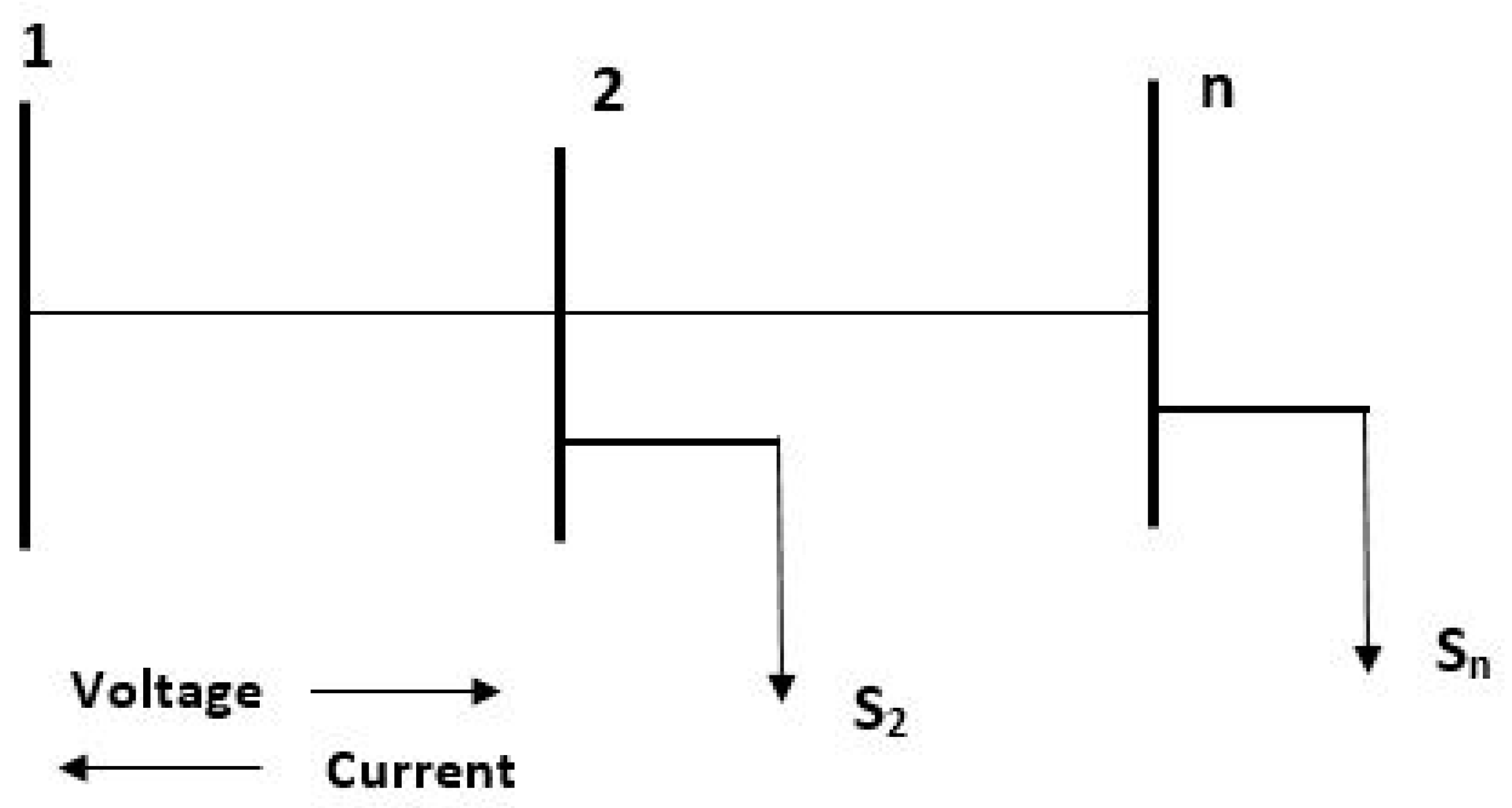
39]. The most suitable algorithm for distribution systems is the backward/forward sweep-based power-flow solution, whose derivation is presented as follows:
With reference to Figure 1, the current of each load can be formulated as
I n = S n V n * = P n j Q n V n
But, to calculate the current of each line starting from the end of the feeder, backward sweep is used:
I n 1 = I n + k = n l i n e I k
In the same way, voltage is calculated using the forward sweep method, starting from the first bus.
V n + 1 = V n Z n l i n e × I n l i n e
The backward and forward sweep modified method uses Kirchhoff’s laws to formulate equations. With the formulated equations, solutions for power flow are obtained without the need to solve the simultaneous equations.
Consider the simple radial distribution line diagram shown in Figure 2. The branch current is denoted by  I n ,   n + 1  and the injected current is denoted by  I n . For simplicity, let  I n ,   n + 1  be ‘B’ and  I n  be ‘I’. With this information,
I 45   = B 4 = I 5
I 34 = B 3 = B 4 + I 4
I 36 = B 5 = I 6
I 23 = B 2 = I 5 + I 4 + I 6 + I 3
I 12 = B 1 = I 23 + I 2
Based on the backward sweep of the branch current equation above, a matrix is formed.
B 1 B 2 B 3 B 4 B 5 = 1       1       1       1       1 0         1       1     1     1 0       0       1       1     1 0       0       0       1       1 0       0       0       0       1 I 1 I 2 I 3 I 4 I 5
The matrix formulated in (30) can be written compactly as
B = B I B C I
Using the same approach as in [40], the branch current to bus voltage is expressed in Figure 1 using forward sweep as follows:
V 2 = V s < 0 I 12 Z 12
V 3 = V 2 I 12 Z 23
V 4 = V 3 I 34 Z 34
V 5 = V 4 I 45 Z 45
V 6 = V 3 I 36 Z 36
From the above equations, it is obvious that the bus voltage is a function of line parameters, source voltage and branch currents. In matrix form,
V s V s V s V s V s V 2 V 3 V 4 V 5 V 6 = Z 12         0         0           0             0 Z 12 Z 23         0       0         0 Z 12 Z 23 Z 34     0         0 Z 12     Z 23 Z 34     Z 45     0 Z 12 Z 23     0         0         Z 56 B 1 B 2 B 3 B 4 B 5
Compactly,
V = B C B V B
Substituting (31) into (38), we get a DG incorporation relationship that involves the bus voltage and injection current as
V = B C B V B I B C I
In a network involving DG, the injected power is given as
S i = S D i S G i
where
  •   S i  = the injected power at the ith bus
  • S D i  = the load power at the ith bus
  • S G i  = the generator power at the ith bus
Since incorporating DG into the network system takes the form of current, then DG at the ith bus is given as
I i = P D i P G i j   Q D i Q G i * V i
The variation in voltage in the DG-incorporated network is given as follows
V K + 1 = B C B V B I B C I K
where
V K + 1 = V 0 V K + 1

2.3. Particle Swarm Optimization (PSO)

In this paper, Particle Swarm Optimization (PSO) was applied to solve multi-objective function presented in Equation (3) which are subjected to the constraints presented in Equations (7)–(9) to analyse the voltage variation and network real power losses while changing the number of DG at the network configuration. Particle swarm optimization (PSO) is inspired by the movement and intelligence of swarms searching for food placed in an unknown location. Each swarm is recognized as a particle or variable X, but vying for a common objective. The optimal position is known individually as a personal best (Pbest) but, in a group, it is known as the global best (Gbest). The particle that each individual represents is known as a possible solution. The search for the optimal solution happens in a search space normally known as a solution space, where other particles must follow the best particle moving ahead, and they change their position and fitness regularly, optimizing their chances of success in finding the best solution.
A particle is represented by the variable X = [x1, x2, x3xn] that would minimize the power losses and maximize the voltage stability or cost and production; this depends on a set objective function. The proposed optimization fitness function is formulated as f(X), where X is known as the position vector that represents the vector model. X is an n-dimension vector since it can be a multi-dimension vector, so n represents the number of variables that can be determined in the set problems. Another variable the particles possess in the search space is velocity, V = [v1, v2, v3vn], which represents the direction of searching. During the iteration process, each particle maintains the best-found position, pbest, individually and the group position, also known as the best position of the group, gbest, and changes its position following the best found positions. The function of f(X), known as the objective function or fitness function, is to assess the performance of the particle’s position in the search space and find an optimal point at the end. This criterion is achieved by employing a number of iterations and updating the position until the maximum or minimum point is reached. The particle position is updated as given below:
X i t + 1 = X i t + V i t + 1
where velocity
V i t + 1 = V i t + C 1 r 1   p i t x i t + C 2 r 2 ( p i g x i t )
where
  • X i t —Particle position
  • V i t —Particle velocity
  • p i t —Best recent individual particle position
  • p i g —Best recent swarm position
  • C1, C2—Cognitive and social parameters
  • r1, r2—Random numbers between 0 and 1
In the Gbest, the velocity of a particle i with the inertia  ω  will be given as
V i t + 1 = w V i t + C 1 r i t P b e s t , i t x i t + C 2 r 2 t [ G b e s t x i t ]
where C1 and C2 are the acceleration coefficients while r1 and r2 denote random values required to maintain the velocity components.

2.4. Proposed Scheme for the Identification of Suitable Locations for DG Placement

The performance of a system dominated by DG is highly influenced by the locations where the DGs are placed in the system. Consequently, a suitable location is where the influence of the DG will positively impact the system; thus, suitable locations for DG placement are of paramount importance. This is because using poor locations for DG placement in a power network could be highly detrimental and uneconomical as this will result in a significant increase in losses and a significant reduction in the system voltage profile. To avoid the aforementioned challenges, this paper suggests the use of a novel approach, the coupling factor (CF) method. This approach is mainly network topology-based and is characterized by simple mathematical formulations. This approach of CF is non-iterative and therefore swiftly identifies weak points suitable for DG placement.
Consider a simple two-bus distribution system, the CF of the line having an impedance of  z j k , connecting bus i and bus j, whose voltages  v j  and  v k  can be easily derived from the system matrix of the coupling strength using the atomic theory concept [41]. According to Alayande et al. in references [42,43,44], the pull–push attractive force matrix, as stated by Coulomb’s law, which represents the coupling strength matrix (CSM) of the transmission line between any two buses  j  and  k  can be modeled by
In terms of the branch admittance between transmission lines  j  and  k  ( y j k ), we can write Equation (47) as
[ C S M ] j k = c ( v j v k ) ( y j k ) 2
where  c  is a constant and  v j  and  v k  are the voltages associated with buses  j  and  k . It is worth noting that the charges associated with buses  j  and  k  are directly proportional to voltages  v j  and  v k , respectively. The introduction of min–max scaling to the off-diagonal elements of the CSM results in a normalized value of the off-diagonal elements of the CSM and is defined as the CF of the node. This is expressed as
C F = [ C S M ] j k m i n [ C S M ] j k m a x [ C S M ] j k m i n [ C S M ] j k
Since the voltage is expected to remain constant and close to unity, it can be seen from Equation (48) that the CSM is directly proportional to the square of the transmission line branch admittance. Hence, the weakest transmission line in any given network can be easily identified. This corresponds to the line associated with the lowest coupling factor (CF).

3. Results and Discussion

This section presents the results obtained for the voltage magnitude and real and reactive power and network losses with and without the integration of DG. In verifying the effectiveness of this approach, the IEEE 33-bus distribution system, whose one-line diagram is shown in Figure 3, was used. The bus data (load) and branch data (line) were obtained from [11,24]. This study was carried out on a system with the following configuration: HP 14” HD Laptop, Intel Core i5-1035G1 (quad-core processor), Intel UHD Graphics, 8GB SDRAM, 256GB SSD, and Matlab 2023b was used as the programming tool.

3.1. Quick Identification of DG Locations

Traditionally, the identification of DG placement is usually carried out using an iterative-based power-flow solution method. This method is associated with various challenges that can hinder the quick identification of locations where DGs could be optimally placed. One of the major challenges associated with iterative-based procedures, which has been of serious concern to power systems researchers, is the convergence issue. Oftentimes, a local optimal solution is obtained instead of a global optimal solution. The information provided by such a solution can be misleading. Another issue associated with the load-flow-based solution is computational and space complexity problems. In order to provide effective solutions to these problems, an alternative coupling factor (CF) method is suggested. Considering the base case scenario, the results obtained using the novel approach of the coupling factor (CF) method for identifying weak points within a system are presented in Table 1.
It can be seen from the results that bus 16 presented the lowest value of CF and, as such, its CF is ranked first. The implication of this is that bus 18 was the weakest bus through which DG integration or placement could be identified to benefit system operations. The next bus, whose value is ranked second, was bus 33, as seen in the results presented in Table 1, and next to bus 33 was bus 32 followed by bus 31 and buses 30, 17, 16, etc. In order to compare the results, the results obtained through the load-flow-based solution are presented in Table 2. As presented in Table 2, the voltage magnitudes are ranked in order of increasing magnitudes. By comparing the results obtained using the two methods as presented in Table 1 and Table 2, it can be seen that these results compare well for the first seven buses (i.e., buses 18, 33, 32, 31, 32, 30, 17 and 16).

3.2. Optimization Results Using PSO without and with DG integration

In considering the integration of DGs into the system, the problem was formulated as a multi-objective function such that the voltage stability was maximized and the power losses were minimized, considering sets of constrained elements using a PSO algorithm. In this paper, six different scenarios were considered based on the network bus CF priority results presented in Table 1 to investigate the influence of DG integration on a radial power system. These scenarios were classified as either an optimal case or an arbitrary case depending on the identified location as specified by the CF results. The first scenario represents the base case where the system topology still remained intact. In this scenario, no DG was installed and the power-flow results represent the steady-state simulation of the system. The results obtained for this scenario are presented in Table 2. In the second scenario, only one DG, whose size was determined using the PSO algorithm, was integrated into the system at bus 18, which was the optimal location as specified by the lowest CF value. The third scenario involved the installation of only one DG, whose location was arbitrarily chosen. In this arbitrary case, bus 16 was used. For the fourth scenario, two DGs were integrated into the system at buses 18 and 33. These were the optimal locations for the integration of two DGs since the CFs associated with buses 18 and 33 were ranked 1 and 2, respectively. The fifth scenario was the arbitrary case where two DGs were installed at buses 16 and 32, which were arbitrarily chosen. The last scenario involved the installation of three DGs at the locations identified by the CF ranking method. These locations were buses 18, 33 and 32 with CF ranking values of 1, 2 and 3, respectively.

3.2.1. Scenario One: Base Case

The results obtained for the base case condition where no DG was integrated into the system, using the PSO method, are presented in Table 3. The results after 200 iterations showed that the maximum and minimum voltages were associated with buses 1 and 18, whose voltage magnitude values were 1.000 pu and 0.8297 pu, respectively.
It can be seen that buses 18, 30, 31, 32 and 33 with voltages 0.8904, 0.8737, 0.8447 and 0.8403, respectively, were outside the prescribed voltage limits of 0.95–1.05 pu. Also, the total power loss obtained through the power-flow analysis using the forward/backward sweep iteration method without the integration of DG was 1.0268 MW. The voltage variation graph for this scenario is presented in Figure 4.

3.2.2. Scenario 2: DG Integration at Bus 18 Using the CF Ranking Method

In this scenario, a DG was installed at bus 18, which was a suitable location, as identified by the CF ranking method presented in Table 1. The voltage profile obtained from the load-flow simulation results using the forward/backward sweep method based on this scenario is presented in Table 4. For the sake of comparison, the results of the voltage profile for the base case scenario are also presented in Table 4. From the voltage profile results obtained, as presented in Table 4, it can be seen that installation of the DG at the identified suitable location (bus 18) significantly improved the voltage profile, and all the bus voltages were within acceptable limits. The minimum voltage magnitude was found to be 0.9843 pu at bus 30, while the maximum voltage magnitude was 1.0200 pu at bus 1. In this case, the power loss obtained stood at 0.3066 MW, which represents a substantial decrease of 70.1% compared to the base case power loss of 1.0268 MW.

3.2.3. Scenario 3: One DG Placed at Bus 16 Based on an Arbitrary Approach

For this scenario, one DG unit, whose placement at bus 16 was arbitrarily selected, was installed. The initial voltage magnitude at the point of connection was 0.9501 pu. After simulations with the PSO, the voltage was found to be optimized when the convergence of the solution was attained. The results of the voltage profile before and after the installation of DG are presented in Table 5. It can be found that voltage magnitudes at all buses were found to be within the prescribed limits. It can, however, be seen that the improvement in the voltage was not all that significant compared to that of the second case in which the location of the DG was based on the CF ranking values. As presented in Table 5, while the minimum voltage magnitude for the system under this scenario was 0.9535 pu at bus 18, the maximum voltage magnitude was 0.9981 pu at bus 2. The system network real power loss obtained after the installation of a DG at bus 16 was found to be 1.1265 MW, which represents about a 9.71% increase in power loss with respect to the base case power loss. Consequently, it can be seen that though the voltage profiles at all buses of the system were slightly enhanced, after the integration of a DG at bus 16, a high increase in power loss was obtained. This implies that bus 16 was not a suitable location for the placement of the DG in order to simultaneously improve the voltage magnitudes at all buses in the system and minimize power losses in the system.

3.2.4. Scenario 4: Two DGs Placed at Buses 18 and 33 Based on the CF Ranking Method

Considering the scenario in which two DGs were placed at the first two buses—18 and 33—identified by the CF ranking method, the results obtained for the system voltage profile are presented in Table 6. Based on the results presented in Table 6, it can be seen that the installation of multiple (two) DGs into the radial distribution network led to significant variation in voltage profiles compared with the base case scenario where no DGs were integrated into the system. As presented, all the voltages were significantly enhanced and all were within the acceptable voltage limits.
As can be seen, the minimum voltage obtained after the integration of the DGs was 0.9890 pu, and this was associated with bus 30, while the maximum voltage of 1.0210 pu was obtained at the slack bus 1. The associated power loss in this case was 0.2348 MW, which is about a 77.1% decrease in power losses within the system. This shows a significant decrease in power loss compared to the power losses obtained in the base case scenario.

3.2.5. Scenario 5: Two DGs Placed at Arbitrary Locations (Buses 16 and 32) Based on an Arbitrary Case

In this scenario, two arbitrary locations where two DGs would be integrated were selected, which were buses 16 and 32. The results obtained for the system voltage profile, considering the system operating condition, are presented in Table 7. It can be seen from the results in Table 7 that the integration of two DGs at locations (buses 16 and 32) that were arbitrarily selected led to a slight improvement in the general voltage profile of the system. Although with this operating condition all the voltage magnitudes lay within the tolerable voltage limits, a decrease in the voltage magnitudes at some buses compared with the base case voltage profile was observed. For example, a decrease in voltage magnitudes was observed for buses 19 to 29. Under this scenario, it can be seen that the system operation was highly influenced by the positions where the DGs were placed. This was expected since the locations where the DGs were placed were arbitrarily selected. Considering this situation, the power loss obtained was 0.9815 MW, which shows a slight decrease of about 4.41% in power losses. Also, from the results presented in Table 7, the minimum voltage magnitude was 0.950 pu, associated with bus 30, while the maximum voltage profile was 1.0100 pu, associated with the reference bus 1.

3.2.6. Scenario 6: Three DGs Placed at Buses 18, 33 and 32 Based on the CF Ranking Method

When the number of DGs integrated into the system was increased to three with locations at buses 18, 33 and 32, the load-flow solution provided the voltage profiles presented in Table 8 for the network under consideration. As can be seen from the results, the voltage profiles were seriously enhanced, thereby providing a better security margin for the system. The minimum voltage was 0.9960 pu at bus 28 while the maximum voltage was 1.0224 pu at bus 14. Also, the power loss associated with this situation was found to be 0.2045 MW. This represents a significant reduction in system power losses of 80%. Compared with the base case scenario, it can be seen that the power loss was also significantly minimized. With the three DGs integrated at these locations (18, 33 and 32) identified by the CF ranking method, the system operation was significantly optimized such that the voltage profile was improved and power losses reduced to the bare minimum. In this scenario, two arbitrary locations where two DGs could be integrated were selected, which were buses 16 and 32. The results obtained for the system voltage profile, considering this system operating condition, are presented in Table 7. It can be seen from the results in Table 7 that the integration of two DGs at locations (buses 16 and 32) that were arbitrarily selected led to a slight improvement in the general voltage profile of the system.
The six scenarios considered and their impact on the network topology are summarized in Table 9. The DG sizes and numbers, DG locations, power losses, minimum voltages and maximum voltage deviations obtained for the six cases and case types considered are presented in Table 9. The six cases considered are depicted in Figure 5 for easy comparison. It can be seen from Figure 5 that the identified locations for DG placement as predicted by the CF method (cases 2, 4 and 6) showed a significant improvement in voltage profiles.

3.3. The Influence of Increasing the Number of DGs on the System Voltage Profile and Power Losses

Table 10 presents a summary of the results obtained for the minimum voltage profile and the associated power losses, considering the placement of the DGs at various positions identified by the CF ranking method. This analysis was performed to investigate the influence of multiple DG integration in a power system on the voltage stability margin as well as the power losses. In this case, up to four DGs, whose sizes were determined using the PSO algorithm, were placed at buses 18, 33, 32 and 31 as presented in Table 10. The minimum voltage magnitudes and the system’s associated power losses are presented. Based on the results presented, it is obvious that there was an enhancement of the voltage profile and a reduction in power losses as the number of DGs was increased up to the installation of three DGs. However, as the number of DGs increased to four, which were placed at buses 18, 33, 32 and 31, the voltage decreased significantly and there was an appreciable increase in power losses. These observations can be explained as follows: When the voltage was within an acceptable range, the distribution network continued to be passive and power flow continued in one direction. But if the number of DGs was continually increased to the point that the DG point of connection with lower voltage had an increased voltage surpassing the allowable range, the network ceased to be passive and power started flowing in multiple directions. As such, the DG installed to augment power losses became an active supply center, which caused fluctuations in the system. This, therefore, diminished the system integrity, which could eventually lead to a total collapse of the distribution network if not quickly checked. This simply implies that a significant increase in the DG penetration in terms of number and size can cause voltage instability, hence the need for monitoring DG sizes and numbers for voltage enhancement and power loss minimization in radial power systems.

3.4. Performance Analysis and Comparison of Methods

The results obtained, using the novel approach suggested in this paper considering the integration of both single and multiple DGs in a radial distribution power system, for loss minimization and voltage profile improvement are compared with the results obtained using different existing methods in this section. Based on single DG integration, the results presented in Table 11 were obtained. The results obtained when multiple DGs were integrated into the system are presented in Table 12. From the single DG integration results presented in Table 11, the results of eight different methods are compared with the results obtained using the non-iterative-based method suggested in this paper. Based on this comparison of results, it can be seen that the IA method in [45], ELF method in [45], hybrid analytical-heuristic method in [46] and ALO method in [47] all identified bus 6 as the optimal location for single DG integration. The VSI-based method in [48] identified bus 30 as the optimal location, while the DAPSO method in [49] and the EVPSO method in [49] identified bus 8 and bus 11, respectively. Although it was found that the power losses were reduced and the voltage profile of the network was enhanced such that none of the system voltage magnitude lay outside the prescribed voltage limits of 0.95–1.05 pu, more improved optimized power losses and voltage profiles were obtained with the non-iterative-based method presented in this paper. In this study, bus 18 was identified as the optimal site for locating the single DG, with a power loss of 102.70 kW before DG integration and 30.70 kW after DG integration. This clearly indicates that a significant reduction in power loss (70.1%) was achieved compared to other existing methods. Furthermore, it can be seen that there was a significant enhancement in the voltage profile based on the method presented in this study, with a minimum voltage of 0.9843 pu. Therefore, it can be seen that the method presented in this paper achieved the minimum voltage and it is associated with the highest percentage of power loss reduction compared to other existing methods.
The results obtained when the influence of multiple DG integration into a network was investigated, using seven different methods for the sake of comparison, are presented in Table 12. From Table 12, it can be seen that with the locations (buses 18, 33 and 32) identified as the sites for integrating the DGs into the network, the method presented in this paper gave the highest percentage reduction of 80.1% in power losses, with a minimum voltage of 0.9960 at bus 28. It can also be seen that the network losses of 1.0268 MW obtained in this study before the integration of DGs is the least when compared to the losses obtained using all other six existing techniques. The implication of this information is that by exploring the use of the method suggested in this study, a better improvement in the voltage with a minimum power loss is obtained.

4. Conclusions

In this paper, a two-stage method for the swift identification of single and multiple DG location and sizing has been presented. A topological-based method that is non-iterative in nature is suggested for the quick location of DG placement in radial distribution systems. This suggested approach was first applied to a system structure in order to identify suitable locations for placing DGs in an optimal manner to reduce the power losses in the system and enhance the voltage security margin of the system. Particle swarm optimization was employed to determine the sizes of the DGs required to be placed at the identified locations. The suggested approach was applied to the IEEE 33-bus test system to test its applicability and effectiveness. The results obtained show that using the identified locations by the CF ranking method, either single DG or multiple DGs can be optimally placed to enhance the voltage profile of a network and minimize network losses. The influence of identifying locations for DG placement with the CF method using both single and multiple DG integration was investigated. It was observed that the voltage profile and power losses of the system were highly influenced by the number of DGs integrated into the system. In other words, as the number of DGs integrated into the system increased, the system voltage profile increased and the power losses were reduced, irrespective of the DG types. However, it is observed, based on the results obtained, that there is a limit to the number of DGs that can be installed in a system depending on the system size. If this number is exceeded, the voltage profile is reduced and network losses increase. The results obtained in this paper were compared with those in the existing literature using both single and multiple DG integration. Based on the comparative analysis, the results obtained from this study show a significant loss reduction of 70.1% when a single DG is integrated while an 80.1% loss reduction is obtained when multiple DGs are integrated. Thus, the method presented in this paper offers superior voltage profile enhancement and power loss minimization using the integration of DGs. The time taken for a solution to be obtained when considering single DG and multiple DG installations was 11.28 s and 19.40 s, respectively.
As part of future work, a comprehensive sensitivity analysis should be carried out to investigate how different network configurations affect reductions in power losses and voltage deviations. Also, future studies should consider incorporating more diverse case studies to demonstrate the effectiveness of the proposed methodology across different types of practical and real-time distribution networks.

Author Contributions

The mathematical formulations and programming in this work were developed within the framework of the doctorate of A.O. He is supervised by Y.H. and co-supervised by J.M. The written manuscript was extensively discussed with the supervisors. All authors have read and agreed to the published version of the manuscript.

Funding

This research received no external funding.

Institutional Review Board Statement

Not applicable.

Informed Consent Statement

Not applicable.

Data Availability Statement

All data used for this study are reported within the manuscript.

Conflicts of Interest

The authors declare no conflicts of interest.

References

  1. Momoh, J.A.; Meliopoulos, S.; Saint, R. Centralized and Distributed Generated Power Systems—A Comparison Approach. In Future Grid Initiative White Paper; ESIG: Reston, VA, USA, 2012; pp. 1–10. Available online: http://pserc.wisc.edu/documents/publications/papers/fgwhitepapers/momoh_future_grid_white_paper_gen_analysis_june_2012.pdf (accessed on 27 October 2023).
  2. Oree, V.; Sayed Hassen, S.Z.; Fleming, P.J. Generation expansion planning optimisation with renewable energy integration: A review. Renew. Sustain. Energy Rev. 2017, 69, 790–803. [Google Scholar] [CrossRef]
  3. Cartelle Barros, J.J.; de Llano Paz, F.; Lara Coira, M.; de la Cruz López, M.P.; del Caño Gochi, A.; Soares, I. New approach for assessing and optimising the environmental performance of multinational electricity sectors: A European case study. Energy Convers. Manag. 2022, 268, 116023. [Google Scholar] [CrossRef]
  4. Owosuhi, A.; Hamam, Y.; Munda, J. Maximizing the Integration of a Battery Energy Storage System–Photovoltaic Distributed Generation for Power System Harmonic Reduction: An Overview. Energies 2023, 16, 2549. [Google Scholar] [CrossRef]
  5. Ackermann, T.; Andersson, G.; Söder, L. Distributed generation: A definition. Electr. Power Syst. Res. 2001, 57, 195–204. [Google Scholar] [CrossRef]
  6. Ettehadi, M.; Ghasemi, H.; Vaez-Zadeh, S. Voltage stability-based DG placement in distribution networks. IEEE Trans. Power Deliv. 2013, 28, 171–178. [Google Scholar] [CrossRef]
  7. Shahzad, M.; Akram, W.; Arif, M.; Khan, U.; Ullah, B. Optimal siting and sizing of distributed generators by strawberry plant propagation algorithm. Energies 2021, 14, 1744. [Google Scholar] [CrossRef]
  8. Win, S.H.; Swe, P.L. Loss minimization of power distribution network using different types of Distributed Generation unit. Int. J. Electr. Comput. Eng. 2015, 5, 918–928. [Google Scholar] [CrossRef]
  9. Antonova, G.; Nardi, M.; Scott, A.; Pesin, M. Distributed generation and its impact on power grids and microgrids protection. In Proceedings of the 2012 65th Annual Conference for Protective Relay Engineers, College Station, TX, USA, 2–5 April 2012; pp. 152–161. [Google Scholar] [CrossRef]
  10. Muthukumar, K.; Jayalalitha, S. Optimal placement and sizing of distributed generators and shunt capacitors for power loss minimization in radial distribution networks using hybrid heuristic search optimization technique. Int. J. Electr. Power Energy Syst. 2016, 78, 299–319. [Google Scholar] [CrossRef]
  11. Werkie, Y.G.; Kefale, H.A. Optimal allocation of multiple distributed generation units in power distribution networks for voltage profile improvement and power losses minimization. Cogent Eng. 2022, 9, 2091668. [Google Scholar] [CrossRef]
  12. Shukla, T.N.; Singh, S.P.; Srinivasarao, V.; Naik, K.B. Optimal sizing of distributed generation placed on radial distribution systems. Electr. Power Compon. Syst. 2010, 38, 260–274. [Google Scholar] [CrossRef]
  13. Alam, A.; Gupta, A.; Bindal, P.; Siddiqui, A.; Zaid, M. Power loss minimization in a radial distribution system with distributed generation. In Proceedings of the International Conference on Power, Energy, Control and Transmission Systems, ICPECTS 2018, IEEE, Chennai, India, 22–23 February 2018; pp. 21–25. [Google Scholar] [CrossRef]
  14. Karimi-Zare, P.; Seifi, H. Maximum allowable penetration level determination of a DG in a distribution network. In Proceedings of the 2012 IEEE International Energy Conference and Exhibition (ENERGYCON), Florence, Italy, 9–12 September 2012; pp. 355–360. [Google Scholar] [CrossRef]
  15. Abri, R.S. Al Voltage Stability Analysis with High Distributed Generation Penetration. Ph.D. Thesis, University of Waterloo, Waterloo, ON, Canada, 2012; p. 134. [Google Scholar]
  16. Wang, J.; Kirtley, J.L.; Carvalho, P.M.S. Factors influencing voltage profiles of distributed-generation-integrated feeders. In Proceedings of the IEEE PES Innovative Smart Grid Technologies Conference (ISGT), Washington, DC, USA, 24–27 February 2013. [Google Scholar] [CrossRef]
  17. Masters, C.L. Voltage rise the big issue when connecting embedded generation to long 11 kv overhead lines. Power Eng. J. 2002, 16, 5–12. [Google Scholar] [CrossRef]
  18. Singh, S.; Østergaard, J.; Jain, N. Distributed generation in power Systems: An overview and key issues. In Proceedings of the 24th Indian Engineering Congress, NIT Surathkal, Kerala, India, 29 March 2009; p. 8. [Google Scholar]
  19. Essallah, S.; Khedher, A. Optimization of distribution system operation by network reconfiguration and DG integration using MPSO algorithm. Renew. Energy Focus 2020, 34, 37–46. [Google Scholar] [CrossRef]
  20. Sireesha, R.; Srinivasa Rao, C.; Vijay Kumar, M. Graph theory based transformation of existing Distribution network into clusters of multiple micro-grids for reliability enhancement. Mater. Today Proc. 2023, 80, 2921–2928. [Google Scholar] [CrossRef]
  21. Shokouhandeh, H.; Latif, S.; Irshad, S.; Kamarposhti, M.A.; Colak, I. Optimal Management of Reactive Power Considering Voltage and Location of Control Devices Using Artificial Bee Algorithm. Appl. Sci. 2022, 12, 27. [Google Scholar] [CrossRef]
  22. Vaziri, M.; Afzal, M.; Zarghami, M.; Yazdani, A.; Vadhva, S.; Tavatli, F. Voltage impacts of dg on distribution grid with voltage regulators and SVCs. IEEE Green Technol. Conf. 2013, 95819, 322–329. [Google Scholar] [CrossRef]
  23. Montoya, O.D.; Gil-González, W.; Orozco-Henao, C. Vortex search and Chu-Beasley genetic algorithms for optimal location and sizing of distributed generators in distribution networks: A novel hybrid approach. Eng. Sci. Technol. Int. J. 2020, 23, 1351–1363. [Google Scholar] [CrossRef]
  24. Selim, A.; Kamel, S.; Alghamdi, A.S.; Jurado, F. Optimal Placement of DGs in Distribution System Using an Improved Harris Hawks Optimizer Based on Single- and Multi-Objective Approaches. IEEE Access 2020, 8, 52815–52829. [Google Scholar] [CrossRef]
  25. Jahromi, M.H.M.; Soleymani, S.; Mozafari, B. Optimal allocation of inverter connected DGs: An objective function to minimize deterioration of transient stability of power system. Int. J. Electr. Power Energy Syst. 2020, 123, 106267. [Google Scholar] [CrossRef]
  26. Ben Hamida, I.; Salah, S.B.; Msahli, F.; Mimouni, M.F. Optimal network reconfiguration and renewable DG integration considering time sequence variation in load and DGs. Renew. Energy 2018, 121, 66–80. [Google Scholar] [CrossRef]
  27. Alanazi, M.S. A MILP model for optimal renewable wind DG allocation in smart distribution systems considering voltage stability and line loss. Alex. Eng. J. 2022, 61, 5887–5901. [Google Scholar] [CrossRef]
  28. Subbaramaiah, K.; Sujatha, P. Optimal DG unit placement in distribution networks by multi-objective whale optimization algorithm & its techno-economic analysis. Electr. Power Syst. Res. 2023, 214, 108869. [Google Scholar] [CrossRef]
  29. Suresh, M.C.V.; Edward, J.B. A hybrid algorithm based optimal placement of DG units for loss reduction in the distribution system. Appl. Soft Comput. J. 2020, 91, 106191. [Google Scholar] [CrossRef]
  30. Huy, P.D.; Ramachandaramurthy, V.K.; Yong, J.Y.; Tan, K.M.; Ekanayake, J.B. Optimal placement, sizing and power factor of distributed generation: A comprehensive study spanning from the planning stage to the operation stage. Energy 2020, 195, 117011. [Google Scholar] [CrossRef]
  31. Yang, Z.; Yang, F.; Min, H.; Tian, H.; Hu, W.; Liu, J. Review on optimal planning of new power systems with distributed generations and electric vehicles. Energy Rep. 2023, 9, 501–509. [Google Scholar] [CrossRef]
  32. Payasi, R.P.; Singh, A.K.; Singh, D. Planning of different types of distributed generation with seasonal mixed load models. Int. J. Eng. Sci. Technol. 2018, 4, 112–124. [Google Scholar] [CrossRef]
  33. Gianto, R.; Iqbal Arsyad, M.; Purwoharjono; Imansyah, F.; Khwee, K.H. Distributed Generation in Electric Power Systems: An Overview and Important Issues. WSEAS Trans. Power Syst. 2023, 18, 172–178. [Google Scholar] [CrossRef]
  34. Gomez, J.C.; Vaschetti, J.; Coyos, C.; Ibarlucea, C. Distributed generation: Impact on protections and power quality. In IEEE Latin America Transactions; IEEE: New York, NY, USA, 2013; Volume 11, pp. 460–465. [Google Scholar]
  35. Csanyi, E. Principles for Controlling Harble. Available online: https://electrical-engineering-portal.com/principles-for-controlling-harmonics (accessed on 17 October 2023).
  36. Abdel-Akher, M.; Ali, A.A.; Eid, A.M.; El-Kishky, H. Optimal size and location of distributed generation unit for voltage stability enhancement. In Proceedings of the IEEE Energy Conversion Congress and Exposition, Phoenix, AZ, USA, 17–22 September 2011; pp. 104–108. [Google Scholar] [CrossRef]
  37. Konstantinos, A. Power quality and economics of integration of distributed generation in LV networks. Master’s Thesis, University of Strathclyde, Glasgow, Scotland, 2004. [Google Scholar]
  38. Kigen, C.; Odero, N.A. Voltage Controller for Radial Distribution Networks with Distributed Generation. Int. J. Sci. Res. Publ. 2014, 4, 1–6. [Google Scholar]
  39. Afolabi, O.; Ali, W.; Cofie, P.; Fuller, J.; Obiomon, P.; Kolawole, E. Analysis of the Load Flow Problem in Power System Planning Studies. Energy Power Eng. 2015, 7, 509–523. [Google Scholar] [CrossRef]
  40. Alsaadi, A.; Gholami, B. An effective approach for distribution system power flow solution. World Acad. Sci. Eng. Technol. 2009, 37, 220–224. [Google Scholar]
  41. Samson, A.; Popoola, O.; Paul, G. e-Prime—Advances in Electrical Engineering, Electronics and Energy A novel non-iterative based framework for quick dynamic assessment of wind energy dominated multi-machine power system. e-Prime Adv. Electr. Eng. Electron. Energy 2023, 5, 100237. [Google Scholar] [CrossRef]
  42. Alayande, A.S.; Jimoh, A.A.; Yusuff, A.A. Identification of critical buses and weak transmission lines using inherent structural characteristics theory. In Proceedings of the Asia-Pacific Power and Energy Engineering Conference, APPEEC, Xi’an, China, 25–28 October 2016; Volume 2016, pp. 1–6. [Google Scholar] [CrossRef]
  43. Alayande, A.S. Solving Power System Problems Based on Network Structural Characteristics; Tshwane University of Technology: Pretoria, South Africa, 2017. [Google Scholar]
  44. Samson, A.A.; Popoola, O.; Mbey, V. An alternative framework for implementing generator coherency prediction and islanding detection scheme considering critical contingency in an interconnected power grid. Int. J. Appl. Sci. Eng. 2022, 19, 1–12. [Google Scholar] [CrossRef]
  45. Baran, M.E.; Wu, F.F. Optimal sizing of capacitors placed on a radial distribution system. IEEE Trans. Power Deliv. 1989, 4, 735–743. [Google Scholar] [CrossRef]
  46. Vatani, M.; Alkaran, D.S.; Sanjari, M.J.; Gharehpetian, G.B. Multiple distributed generation units allocation in distribution network for loss reduction based on a combination of analytical and genetic algorithm methods. IET Gener. Transm. Distrib. 2016, 10, 66–72. [Google Scholar] [CrossRef]
  47. Ali, E.S.; Abd Elazim, S.M.; Abdelaziz, A.Y. Ant Lion Optimization Algorithm for optimal location and sizing of renewable distributed generations. Renew. Energy 2017, 101, 1311–1324. [Google Scholar] [CrossRef]
  48. Karunarathne, E.; Pasupuleti, J.; Ekanayake, J.; Almeida, D. Network loss reduction and voltage improvement by optimal placement and sizing of distributed generators with active and reactive power injection using fine-tuned pso. Indones. J. Electr. Eng. Comput. Sci. 2020, 21, 647–656. [Google Scholar] [CrossRef]
  49. Manafi, H.; Ghadimi, N.; Ojaroudi, M.; Farhadi, P. Optimal Placement of Distributed Generations in Radial Distribution Systems Using Various PSO and DE Algorithms. Electron. Electr. Eng. 2013, 19, 53–57. [Google Scholar] [CrossRef]
  50. Montoya, O.D.; Molina-Cabrera, A.; Chamorro, H.R.; Alvarado-Barrios, L.; Rivas-Trujillo, E. A hybrid approach based on socp and the discrete version of the sca for optimal placement and sizing dgs in ac distribution networks. Electronics 2021, 10, 26. [Google Scholar] [CrossRef]
Figure 1. A simple distribution network to demonstrate the backward and forward sweep method.
Applsci 14 01077 g001
Figure 2. Radial distribution network showing the voltage at each bus.
Applsci 14 01077 g002
Figure 3. IEEE 33-bus radial network [23,43].
Applsci 14 01077 g003
Figure 4. Base case voltage profile for the IEEE 33-bus system.
Applsci 14 01077 g004
Figure 5. Comparison of the six scenarios for identifying optimal locations for DG placement.
Applsci 14 01077 g005
Table 1. Bus coupling factor (CF) for identifying weak buses in the IEEE 33-bus distribution system.
Bus No.CFCF RankingBus No.CFCF Ranking
10.765533180.10231
20.634224190.413512
30.525516200.574320
40.475315210.643225
50.427314220.425313
60.546717230.572418
70.584321240.711128
80.631323250.20948
90.644726260.753232
100.385410270.731430
110.403511280.722329
120.35259290.745331
130.573419300.16215
140.589122310.13504
150.685727320.13033
160.16877330.10542
170.16226
Table 2. Voltage profiles for identifying weak buses in the IEEE 33-bus distribution system.
Bus No.Voltage
(pu)
Voltage
Ranking
Bus No.Voltage
(pu)
Voltage
Ranking
11.000033180.82971
20.995232190.994431
30.982427200.988530
40.970423210.987329
50.967322220.986126
60.965121230.976925
70.962019240.970724
80.957416250.977626
90.956315260.963220
100.95079270.960818
110.951610280.959317
120.952211290.954714
130.953112300.89045
140.953513310.87374
150.95028320.84473
160.95017330.84032
170.95006
Table 3. Results when no DG was integrated into the system.
Number of Iterations200
DG locationnil
Minimum voltage0.8614 pu
Maximum voltage1.0000 pu
Network real power3715 kW
Network reactive power2290 kVar
Power loss without optimization1.0268 MW
Table 4. Voltage profile without and with the integration of one DG at bus 18 into the IEEE 33-bus distribution system using the CF ranking method.
Bus No.Bus Voltage Profile with No DG (pu)Bus Voltage Profile with DG (pu)Bus No.Bus Voltage Profile with No DG (pu)Bus Voltage Profile with DG (pu)
11.00001.0200180.82970.9858
20.99521.0010190.99440.9936
30.98241.0142200.98850.9991
40.97041.0009210.98731.0120
50.96731.0102220.98611.0073
60.96511.0012230.97691.0108
70.96201.0110240.97071.0154
80.95741.0009250.97761.0103
90.95631.0108260.96321.0148
100.95071.0102270.96081.0016
110.95161.0094280.95930.9946
120.95220.9983290.95471.0019
130.95310.9934300.89040.9843
140.95351.0005310.87370.9987
150.95021.0021320.84470.9878
160.95010.9875330.84030.9982
170.95000.9887
Table 5. Voltage profile without and with the integration of one DG at arbitrarily selected bus 16 in the IEEE 33-bus distribution system.
Bus No.Bus Voltage Profile with No DG (pu)Bus Voltage Profile with DG (pu)Bus No.Bus Voltage Profile with No DG (pu)Bus Voltage Profile with DG (pu)
11.00000.9950180.82970.9535
20.99520.9981190.99440.9835
30.98240.9882200.98850.9824
40.97040.9867210.98730.9853
50.96730.9942220.98610.9837
60.96510.9568230.97690.9758
70.96200.9787240.97070.9744
80.95740.9745250.97760.9753
90.95630.9784260.96320.9877
100.95070.9867270.96080.9814
110.95160.9876280.95930.9735
120.95220.9865290.95470.9886
130.95310.9876300.89040.9624
140.95350.9676310.87370.9746
150.95020.9768320.84470.9648
160.95010.9765330.84030.9735
170.95000.9756
Table 6. Voltage profile without and with the integration of two DGs at suitable locations (buses 18 and 33) based on the CF ranking values in the IEEE 33-bus distribution system.
Bus No.Bus Voltage Profile with No DG (pu)Bus Voltage Profile with DG (pu)Bus No.Bus Voltage Profile with No DG (pu)Bus Voltage Profile with DG (pu)
11.00001.0210180.82970.9899
20.99521.0031190.99440.9992
30.98241.0101200.98850.9924
40.97041.0020210.98730.9946
50.96731.0110220.98610.9901
60.96511.0032230.97690.9899
70.96201.0250240.97070.9942
80.95741.0024250.97760.9946
90.95631.0109260.96320.9973
100.95071.0046270.96080.9963
110.95161.0153280.95930.9972
120.95221.0026290.95470.9920
130.95311.0137300.89040.9890
140.95350.9835310.87370.9948
150.95020.9964320.84470.9943
160.95010.9824330.84030.9896
170.95000.9894
Table 7. Voltage profile without and with the integration of two DGs at arbitrarily selected locations (buses 16 and 32) in the IEEE 33-bus distribution system.
Bus No.Bus Voltage Profile with No DG (pu)Bus Voltage Profile with DG (pu)Bus No.Bus Voltage Profile with No DG (pu)Bus Voltage Profile with DG (pu)
11.00001.0100180.82970.9724
20.99520.9984190.99440.9624
30.98240.9841200.98850.9621
40.97040.9846210.98730.9617
50.96730.9943220.98610.9578
60.96510.9853230.97690.9673
70.96200.9835240.97070.9635
80.95740.9885250.97760.9732
90.95630.9824260.96320.9624
100.95070.9735270.96080.9587
110.95160.9754280.95930.9617
120.95220.9736290.95470.9636
130.95310.9674300.89040.9500
140.95350.9646310.87370.9576
150.95020.9634320.84470.9563
160.95010.9684330.84030.9583
170.95000.9635
Table 8. Voltage profile without and with the integration of three DGs at locations (buses 18, 33 and 32) selected using the CF ranking method in the IEEE 33-bus distribution system.
Bus No.Bus Voltage Profile with no DG (pu)Bus Voltage Profile with DG (pu)Bus No.Bus Voltage Profile with No DG (pu)Bus Voltage Profile with DG (pu)
11.00001.0190180.82970.9990
20.99521.0001190.99441.0001
30.98241.0103200.98850.9994
40.97041.0120210.98730.9964
50.96731.0130220.98610.9976
60.96511.0056230.97690.9975
70.96201.0201240.97070.9968
80.95741.0046250.97760.9963
90.95631.0114260.96320.9983
100.95071.0053270.96080.9988
110.95161.0140280.95930.9960
120.95221.0064290.95470.9984
130.95311.0125300.89040.9967
140.95351.0224310.87370.9997
150.95021.0135320.84470.9989
160.95010.9969330.84030.9966
170.95000.9986
Table 9. Summary of the voltage profiles and power losses with and without DG installation.
Case No.Case TypeNo. of DGsDG Size (MW)DG LocationPower Loss (MW)Minimum Voltage (pu)
1Base Case00NA1.02680.8297 (bus 18)
2Optimal Case12180.30660.9843 (bus 30)
3Arbitrary Case12161.12650.9535 (bus 18)
4Optimal Case22, 1.06418, 330.23480.9890 (bus 30)
5Arbitrary Case22, 1.06416, 320.98150.9500 (bus 30)
6Optimal Case32, 1.04, 1.6418, 33, 320.20450.9960 (bus 28)
Table 10. Influence of increasing the number of DGs on the system voltage profile and power losses.
No. of DGsDG Sizes (MW)DG LocationsPower Loss (MW)Minimum Voltage
00NA1.02680.8297 (bus 18)
12180.30660.9843 (bus 30)
22, 1.0418, 330.23480.9890 (bus 30)
32, 1.04, 2.6418, 33, 320.20450.9960 (bus 28)
42, 1.04, 2.64, 3.0818, 33, 32, 310.35020.9063 (bus 27)
Table 11. Comparison of the results obtained with the existing methods for installing a single DG.
MethodLocationDG Size (MW)Power Loss with No DG (kW)Power Loss with Multiple DGs (MW)Power Loss Reduction (%)Minimum Voltage (pu)
LSF [45]Bus 180.743 146.82--
Hybrid analytical-heuristic [46]62.707-99.22-0.9530 @bus 18
IA [45]62.601210.98111.11--
EVPSO [49]110.763210.98140.19033.550.9604
ELF [45]62.601210.98111.11--
DAPSO [49]81.212210.98127.1739.70.9635
ALO [47]60.850210.98103.0551.150.9503 @bus 18
VSI-based [48]301.243210.0781.5060.36-
This paperBus 182.000102.6830.7070.10.9843 @bus 30
Table 12. Comparison of the results obtained with the existing methods for multiple DG integration.
MethodLocation (Bus Nos.)DG Size (MW)Power Loss with No DG (MW)Power Loss with Multiple DGs (MW)Power Loss (%)Min. Voltage
Hybrid CBGA-VSA [23]13, 24, 302.945-0.72865.50.9687 @bus 33
IHHO [24]14, 24, 302.9232.10980.72865.50.9790 @bus 18
ALO [47]13, 302.0412.10980.82660.80.9732 @bus 33
GA [46]30, 132.190-0.81862.50.9734 @bus 33
Hybrid DSCA-SOCP [50]13, 24, 302.9452.10990.72865.5-
SPPA [7]3, 63.4952.10990.63769.40.9929 @bus 18
VSI-based [48]30, 251.4922.10070.72965.29-
This paper18, 33, 322.6401.02680.204580.10.9960 @bus 28
Disclaimer/Publisher’s Note: The statements, opinions and data contained in all publications are solely those of the individual author(s) and contributor(s) and not of MDPI and/or the editor(s). MDPI and/or the editor(s) disclaim responsibility for any injury to people or property resulting from any ideas, methods, instructions or products referred to in the content.

