A Novel Robust Control System Design and Its Application to Servo Motor Drive

Abstract

This paper proposes a new control system by integrating integral state feedback control and sliding mode control to eliminate the influences from the reference input change, external load, and parameter variations. For most control systems, integral action is used to overcome the reference input change and external load. However, its control performance cannot be guaranteed. State feedback control is used to dominate the pole location of the closed-loop control system. However, the system parameters determine their pole locations and may change due to uncertainties. Thus, the characteristics of the closed-loop control system are changed. Sliding mode control is used to compensate for the effect of the parameter variations and make the system invariant. The resulting system combines linear state feedback and sliding mode control to guarantee the desired performance. This shows that the proposed system can be easily applied and designed. A servo control system is used to demonstrate the performance, and simulations and experiments are carried out to evaluate the newly defined structure. They show that the strategies and control design can reach robust performance even with uncertainties or external load, and the chattering of the sliding mode control can be minimized.

1. Introduction

Due to the simple structure and easy adjustment of control parameters, control systems designed using a PI/PD/PID controller in cascade are usually adopted to compensate for variations in reference input and external disturbances. Many turning methods, including online and offline strategies, have been developed to adjust the control parameters manually or automatically. Over the years, many commercial controllers have been designed and produced based on digital signal processing (DSP) technology, and they are functionally diverse but cheap. Nevertheless, as usual, the cascade mode is still prevalent, and the controller style is mainly still in a commercial controller’s PI/PD/PID functions. Many modern control strategies are sometimes applied to commercial controller design due to the necessity of state feedback, and most of the systems are different from each other, which causes some modern controllers to be in the sense of a case study. For this purpose, we wanted to design an easy application control structure for the control system design such as the well-known commercial controllers, and the designed system is robust to the reference change and added disturbance.

State feedback control has the characteristics of an easily understood and implemented structure. The system controlled by the state feedback has the properties of arbitrarily pole assignment, while the system is controllable. On the other hand, a state observer can be designed to estimate the system states and put them back to the controller if some states are not directly accessible. However, it is weak in facing external load or reference input variation. For the control end, zero steady-state error is desired for most control objects. Integral action or disturbance estimation in state feedback system design is used to overcome these drawbacks. Integral action has the property of the cascade PI control structure. Once the system’s states (usually the error of the state) cannot be forced to the desired state (usually the origin) by way of the controller, steady-state errors exist. An integral control that will integrate the errors and increase/decrease the control output to force the system states back to the desired state is designed to eliminate the errors. If the resulting system is stabilizable, the system will finally reach and stop at the desired state. State feedback control with/without integral action is widely applied to motor drive systems and power converter design. Example studies include a DC motor [1,2,3,4,5,6], a permanent magnet synchronous motor [7,8,9], a stepper motor [10,11], a BLDC [12], a robot [13,14,15,16], a power converter [17,18,19,20,21,22], a magnetic levitation system [23], an unmanned surface vehicle [24,25], landing control [13,26], a UAV vehicle [27], and a two-tank system [28].

The system’s parameters determine the default system performance using the state feedback control structure. The poles of the closed-loop system vary due to the variations in system parameters. The effects mentioned above may not cause severe deterioration to reduce steady-state performance. However, some system considerations are specified, such as minimum overshoot, rising time, settling time, or delay time. For those conditions, the system’s performance may not fit the requirements.

Thus, to make the system performance invariant is essential. Sliding mode control (SMC) or variable structure control (VSC) is one of the solutions to make a system invariant to the parameter variations. A system controlled by SMC with invariant property considerations can be found in [11,15,29].

There are two steps for the SMC controller design. First, one must determine the system performance according to the transient specifications, such as the rising time, settling time, delay time, and maximum overshoot. Some situations regarding reaching transient requirements are placing the system poles at specified locations to reach the desired performance. Pole placement [3,11,15] or the linear quadrature method [5,14,15,30,31] can be used to determine the locations of system poles. Second, it is necessary to determine the control law to cause the system to move onto the sliding surface, stay on it, and slide to the desired location. Typically, a sliding surface is designed to have the performance to fit the system’s requirements. However, the chattering phenomenon due to fast switching inputs cannot be avoided to keep the states on the sliding surface, which may degrade system performance [12]. Chattering eliminations are considered in [5,8,9,23,26,27,32]. Estimating the load torque or determining the control law through the boundary layer can reduce this chattering [9,23,24,27].

A servo motor control system usually constitutes the external load or disturbance, and nonlinear phenomena such as backlash or dead-band also give rise to steady-state error. The proposed control structure is thus used for the position control of the servo motor system. The design process and simulation results are given to show the performance of the proposed system.

The other contents of the paper are as follows. Section 2 presents the integral state feedback control design. Section 3 adds the sliding mode control to the existing state feedback system to improve the invariance property. The determination of SMC control law is shown in Section 4. The developed control system applied to the position control of the servo drive system is shown in Section 5. The simulation and experimental results and discussions are given in Section 6 and Section 7. Finally, the conclusions are given in Section 8.

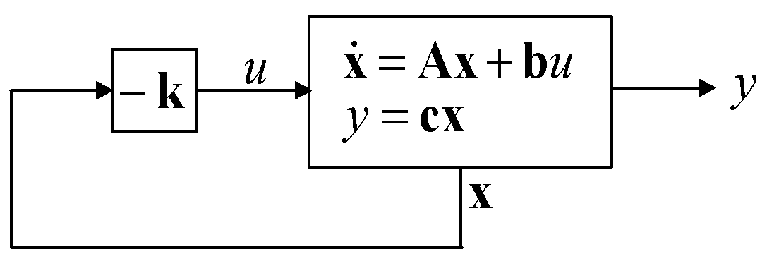
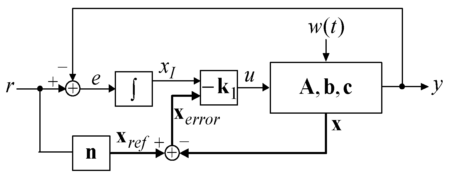
2. Controller Design Using State Feedback and Integral Action

A conventional state feedback controller with full state feedback is shown in Figure 1. An nth-order single input/single output system is represented as the state variable form, as Equation (1) shows.

$$\begin{array}{l}\dot{x}=Ax+bu\\ y=cx\end{array}$$

(1)

where $A\in R^{n\times n}$, $b\in R^{n\times 1}$, $c\in R^{n\times 1}$, and $x\in R^{n\times 1}$ are the system states. If the system is controllable, state feedback can be used to stabilize the system, and these control law design methodologies, such as pole placement or the linear quadratic (LQ) technique, can be used to decide the feedback control gain. Assume that the control gain $k\in R^{n\times 1}$ is decided, the control law can be set as:

$$u=-k^{\mathrm{T}}x$$

(2)

and the system state equation with state feedback can be represented as:

$$\begin{array}{ll}\dot{x}& =Ax+bu\\ & =Ax+b(-k^{\mathrm{T}}x)\\ & =A_c\end{array}$$

(3)

For a velocity-type control system, a system with non-zero reference input, or a system with external perturbation/disturbance, a pure state feedback control law, Equation (2), cannot wholly compensate for those non-ideal cases and will result in a steady-state error. For the control end, integral action is adopted to eliminate those phenomena [33]. Consider the system shown in the block diagram of Figure 2, designed under the integral state feedback compensation control. The system is represented as follows:

$$\begin{array}{l}\dot{x}=Ax+bu+w\\ y=cx\end{array}$$

(4)

The system is subjected to the reference input $r(t)$ and input disturbance/perturbation $w(t)$, where:

$$w(t)={\left[\begin{array}{cccc}0& \cdots & 0& w(t)\end{array}\right]}^{\mathrm{T}}$$

(5)

Define the new reference states as $x_{ref}$, and it has the form:

$$x_{ref}={[\begin{array}{cccc}{x}_{1ref}& \cdots & x_{\mathrm{n}-1ref}& x_{\mathrm{n}ref}\end{array}]}^{\mathrm{T}}$$

(6)

and

$$x_{ref}=nr$$

(7)

where $n\in R^{n\times 1}$ and $x_{ref}\in R^{n\times 1}$ are the desired system states in the steady state to the control. The state’s error and derivative are defined as:

$$\begin{array}{cc}{x}_{error}& =x_{ref}-x\hfill \\ & =nr-x\hfill \end{array}$$

(8)

$$\begin{array}{cc}{\dot{x}}_{error}& ={\dot{x}}_{ref}-\dot{x}\hfill \\ & =n\dot{r}-\dot{x}\hfill \\ & =-\dot{x}\hfill \end{array}$$

(9)

An integrator that accepts the differences between the reference input and system output is added to eliminate the steady-state error, and the integrator can be set as

$$\begin{array}{cc}{\dot{x}}_{\mathrm{I}}& =r-y\hfill \\ & =r-cx\hfill \end{array}$$

(10)

The control law design can be accomplished by state feedback to the augmented system, Equations (9) and (10). Assume the new system states are:

$$z=\left[\begin{array}{c}{x}_{\mathrm{I}}\\ x_{error}\end{array}\right]$$

(11)

The augmented system state matrix can be represented as:

$$\begin{array}{cc}\dot{z}& =\left[\begin{array}{c}{\dot{x}}_{\mathrm{I}}\\ {\dot{x}}_{error}\end{array}\right]=\left[\begin{array}{cc}0& -c\\ 0& -A\end{array}\right]\left[\begin{array}{c}{x}_{\mathrm{I}}\\ x\end{array}\right]+\left[\begin{array}{c}0\\ -b\end{array}\right]u+\left[\begin{array}{c}r\\ -w\end{array}\right]\hfill \\ & =A_{1}z+b_{1}u+w_1\hfill \end{array}$$

(12)

where the reference inputs are assumed constant in the control process.

Regarding the augmented systems (12), the state feedback control law can be designed according to the assignment of characteristic roots by the feedback gain, $k_1$:

$$u=-k_1^{\mathrm{T}}z$$

(13)

and the resulting equivalent state matrix is:

$$A_{\mathrm{c}1}=A_1-b_1{k}_1^{\mathrm{T}}$$

(14)

Based on the assumption of a controllable canonical form of the controlled system, the system state reference is easy to decide. For a constant reference input system, $r\in \mathrm{const}$, we have the system state references as:

$$\begin{array}{l}{x}_{ref}=nr\\ ={\left[\begin{array}{cccc}1& 0& \cdots & 0\end{array}\right]}^{\mathrm{T}}r\end{array}$$

(15)

If the controlled system is a regulator one, the system’s states will finally reach zero, except the state $x_I$.

We consider a general second-order single input/single output system represented in the controllable canonical form:

$$\begin{array}{l}\left[\begin{array}{c}{\dot{x}}_1\\ {\dot{x}}_2\end{array}\right]=\left[\begin{array}{cc}0& 1\\ -a_1& -a_2\end{array}\right]\left[\begin{array}{c}{x}_1\\ x_2\end{array}\right]+\left[\begin{array}{c}0\\ b\end{array}\right]u+\left[\begin{array}{c}0\\ w\end{array}\right]\\ y=\left[\begin{array}{cc}1& 0\end{array}\right]\left[\begin{array}{c}{x}_1\\ x_2\end{array}\right]\end{array}$$

(16)

The detailed block diagram of the controlled system, Equation (16), and the augmented state feedback controller are demonstrated in Figure 3, where state feedback gains $k_1={\left[\begin{array}{ccc}{k}_1& k_2& k_3\end{array}\right]}^{\mathrm{T}}$ and integrator adopted to eliminate the steady-state error have been added. The new controlled state is assumed as:

$$\begin{array}{cc}z& ={\left[\begin{array}{ccc}{z}_1& z_2& z_3\end{array}\right]}^{\mathrm{T}}\hfill \\ & ={\left[\begin{array}{ccc}{\displaystyle \int z_{2}dt}& r-x_1& -x_2\end{array}\right]}^{\mathrm{T}}\hfill \end{array}$$

(17)

where integrator is set as:

$${\dot{z}}_1=r-x_1=z_2,$$

(18)

The control law is shown in (13).

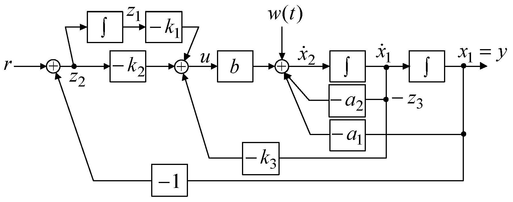
3. Sliding Mode Control Design for a Class of Linear System Models with Perturbations

The following will add the sliding mode control structure to the linear model-represented system. As shown in (13), the integral state feedback control system has the control law $u=-k_1^{\mathrm{T}}z$. The system with the linear control law can eliminate the steady-state error from the reference input and external disturbance input. However, transient performance defined in (14) cannot be guaranteed if the system has parameter variation, i.e., the resulting eigenvalues of the closed-loop system will not be the designed ones. A system with external disturbance and parameter variations included is represented as follows:

$$\dot{z}=(A_1+\Delta A_1)z+(b_1+\Delta b_1)u+w$$

(19)

where $\Delta A_1$ and $\Delta b_1$ are variations in $A_1$ and $b_1$ and $(b_1+\Delta b_1)$ does not change the sign of $b_1$ to maintain controllability. The variations and disturbances in (19) can be lumped and expressed as:

$$p=\Delta A_{1}z+\Delta b_{1}u+w$$

(20)

When the system is expressed in a controllable canonical form, the lumped perturbation can be in the following format:

$$p={\left[\begin{array}{cccc}0& 0& \cdots & \tilde{p}\end{array}\right]}^{\mathrm{T}}$$

(21)

The SMC control is added to recover the system with the desired transient performance as defined by the equivalent system state, $A_{c1}$. First, with a constant vector $g$, where $g^{\mathrm{T}}{b}_1\ne 0$ [11,29], a sliding surface

$$\sigma (t,z)=g^{\mathrm{T}}(z-z_0)-g^{\mathrm{T}}{A}_{c1}{\displaystyle \int z(t)dt}$$

(22)

is used to determine an extra control law, $u_{smc}$. For the closed-loop system (3) under nominal conditions (without the uncertainty, perturbation, and load), with an initial value $x_0$, $\sigma (t,x)=0$ for $t\ge 0$, i.e., the system states are initially on the sliding surface and will stay on it for the entirety of the next proceeding time. However, this is not for a perturbed system (19). Extra control effort is needed to make and keep the states on the sliding surface as a nominal system does.

The extra control law is defined as:

$$u_{smc}=-q\mathrm{sgn}(\sigma )$$

(23)

where sgn(·) is the sign function and $q$ is a positive scalar constant defined as:

$$\frac{q}{b}>{\left|\tilde{p}\right|}_{\max }$$

(24)

where ${\left|\tilde{p}\right|}_{\max }$ is the upper bound of the total perturbation. Then, the total control law for the augmented system is:

$$u=u_L+u_{smc}=-k_1^{\mathrm{T}}z-q\mathrm{sgn}(\sigma )$$

(25)

where $u_L$ is the linear state feedback control. The second part of (25) in the control structure mainly guarantees transient performance since the integral action can ensure steady-state performance. Furthermore, the chattering phenomenon due to the switching control law of $u_{smc}=-q\mathrm{sgn}(\sigma )$ must be solved to let the steady-state performance fit the requirement as a linear control system does.

4. The Determination of Sliding Mode Control Law

The second part, $u_{smc}=-q\mathrm{sgn}(\sigma )$, of (25) is used to guarantee the existence of sliding conditions. Typically, a large quantity of $q$ is chosen to reach the desired performance, with it invariant to perturbation and disturbance. However, this is the primary source leading to chattering.

The action of the integrator can overcome the total perturbation (20). To consider the output, $z_1(t)$, of the integrator by the inputs of reference r(t) and disturbance $w(t)$:

$$Z_1(s)=\frac{s^2+(a_2+b{k}_3)s+a_1}{s^3+(a_2+b{k}_3)s^2+(a_1-b{k}_2)s-b{k}_1}\times R(s)+\frac{-1}{s^3+(a_2+b{k}_3)s^2+(a_1-b{k}_2)s-b{k}_1}\times W(s)$$

(26)

If the two inputs are assumed as step signals,

$$R(s)=\frac{r}{s} \mathrm{and} W(s)=\frac{w}{s}$$

(27)

then

$$\underset{t\to \infty }{\lim }{z}_1(t)=\frac{a_{1}r-w}{-b{k}_1}$$

(28)

With the same procedures, we have the following results:

$$\underset{t\to \infty }{{\displaystyle \lim }}{z}_2(t)=\underset{t\to \infty }{{\displaystyle \lim }}e(t)=0$$

(29)

and

$$\underset{t\to \infty }{{\displaystyle \lim }}{z}_3(t)=0$$

(30)

i.e., the total perturbations of reference input and external disturbances exist at the output of the integrator. Through the linear control part, $u_L=-k_1^{\mathrm{T}}z$, the steady-state output of the controller is from the state $z_1$ only, which can eliminate the total perturbations.

However, the transient response for the integral state feedback control cannot be guaranteed due to the uncertainties of parameters and external load. The second part of (25) is used to keep the state, $z$, on the sliding surface.

The main weak point of SMC control is the chattering phenomenon due to the sign function. Choosing a big value of $q$ easily leads to the occurrence of sliding mode. On the contrary, the performance of sliding mode control is destroyed due to chattering, especially under steady-state conditions. Thus, the design of $q$ should be considered for the steady-state performance. The control law of (23) is modified as

$$-q\mathrm{sgn}(\sigma )=-q\frac{\sigma }{\left|\sigma \right|+\epsilon }$$

(31)

to solve the problem of chattering. In (31), $\epsilon$ is a small positive value and $q$ is chosen to fit the inequality of (24). With the defined control law (31), once the system states are kept on the sliding surface, the extra control law becomes linear control, which avoids the occurrence of chattering.

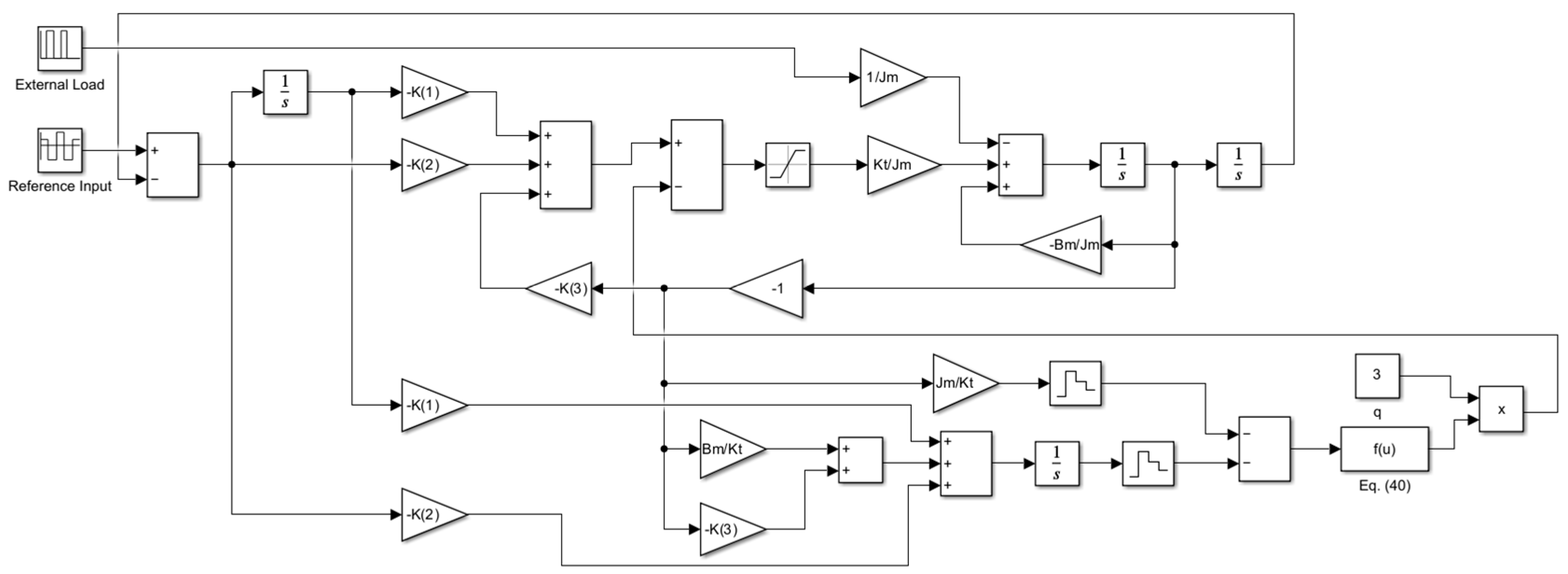
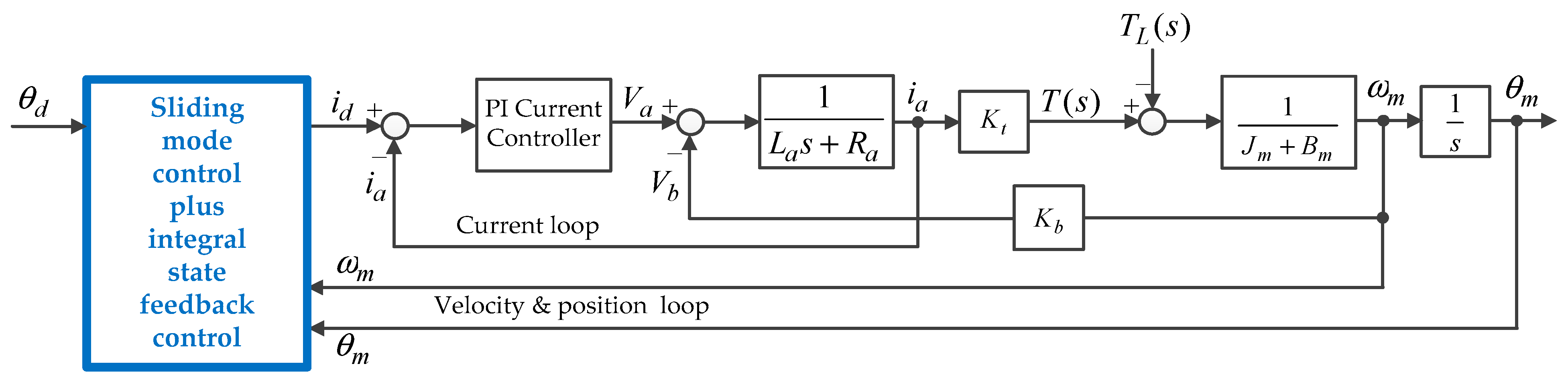
5. Application to the Servo Motor Drive System

Consider the servo motor positioning system expressed as:

$$\begin{array}{cc}\left[\begin{array}{c}{\dot{\theta }}_m\\ {\dot{\omega }}_m\end{array}\right]& =\left[\begin{array}{cc}0& 1\\ 0& -B_m/J_m\end{array}\right]\left[\begin{array}{c}{\theta }_m\\ {\omega }_m\end{array}\right]+\left[\begin{array}{c}0\\ K_T/J_m\end{array}\right]u-\left[\begin{array}{c}0\\ T_L/J_m\end{array}\right]\\ & =Ax+bu+w\hfill \end{array}$$

(32)

$$y={\theta }_m=\left[\begin{array}{cc}1& 0\end{array}\right]\left[\begin{array}{c}{\theta }_m\\ {\omega }_m\end{array}\right]=cx$$

(33)

where $J_m$ is the motor rotor inertia, $B_m$ is the motor viscous, $K_T$ is the torque constant, $T_L$ is the external load, and ${\theta }_m$ and ${\omega }_m$ are the motor angular and motor velocity, respectively. The reference input, $r={\theta }_{md}$, is assumed, and the reference is set as

$$x_{ref}=\left[\begin{array}{c}r\\ 0\end{array}\right]$$

(34)

to define the new state, $z$, as:

$$z=\left[\begin{array}{c}{z}_1\\ z_2\\ z_3\end{array}\right]=\left[\begin{array}{c}{x}_I\\ r-{\theta }_m\\ -{\omega }_m\end{array}\right]$$

(35)

where $z_1$ is from the integrator defined to estimate the total perturbations whenever a system is in a steady state.

$$\begin{array}{cc}\hfill {\dot{z}}_1& =r-{\theta }_m=z_2\hfill \\ \hfill {\dot{z}}_2& =\dot{r}-{\dot{\theta }}_m=-{\omega }_m=z_3\hfill \\ \hfill {\dot{z}}_3& =-{\dot{\omega }}_m=\frac{B_m}{J_m}{\omega }_m+\frac{T_L}{J_m}-\frac{K_T}{J_m}u=-\frac{B_m}{J_m}{z}_3+\frac{T_L}{J_m}-\frac{K_T}{J_m}u\hfill \end{array}$$

(36)

Define the linear control law as $u=-k{}_1{}^{\mathrm{T}}z=-\left[\begin{array}{ccc}{k}_1& k_2& k_3\end{array}\right]z$ and one has:

$$\begin{array}{cc}\dot{z}& =A_{1}z+b_1{u}_1+w_1\hfill \\ & =\left[\begin{array}{ccc}0& 1& 0\\ 0& 0& 1\\ 0& 0& -B_m/J_m\end{array}\right]\left[\begin{array}{c}{z}_1\\ z_2\\ z_3\end{array}\right]+\left[\begin{array}{c}0\\ 0\\ -K_T/J_m\end{array}\right]\left[-\begin{array}{ccc}{k}_1& -k_2& -k_3\end{array}\right]\left[\begin{array}{c}{z}_1\\ z_2\\ z_3\end{array}\right]+\left[\begin{array}{c}0\\ 0\\ T_L/J_m\end{array}\right]\hfill \\ & =\left[\begin{array}{ccc}0& 1& 0\\ 0& 0& 1\\ k_1{K}_T/J_m& k_2{K}_T/J_m& -B_m/J_m+k_3{K}_T/J_m\end{array}\right]z+\left[\begin{array}{c}0\\ 0\\ T_L/J_m\end{array}\right]=A_{\mathrm{cl}}z+\left[\begin{array}{c}0\\ 0\\ T_L/J_m\end{array}\right]\hfill \end{array}$$

(37)

The feedback control $k_1$ can be used to determine the desired system poles under the integral state feedback control.

Thus, the switching control part can be designed by assigning the sliding surface as

$$\sigma (z_1,z_2,z_3,t)=b_1^{-1}(z-z_0)-b_1^{-1}{A}_c{\displaystyle \int zdt}$$

(38)

and incorporated with the control law (31). The vector $g$ in (22) is replaced by $b_1^{-1}$ since the control structure is defined as $g^{\mathrm{T}}{b}_1=1$.

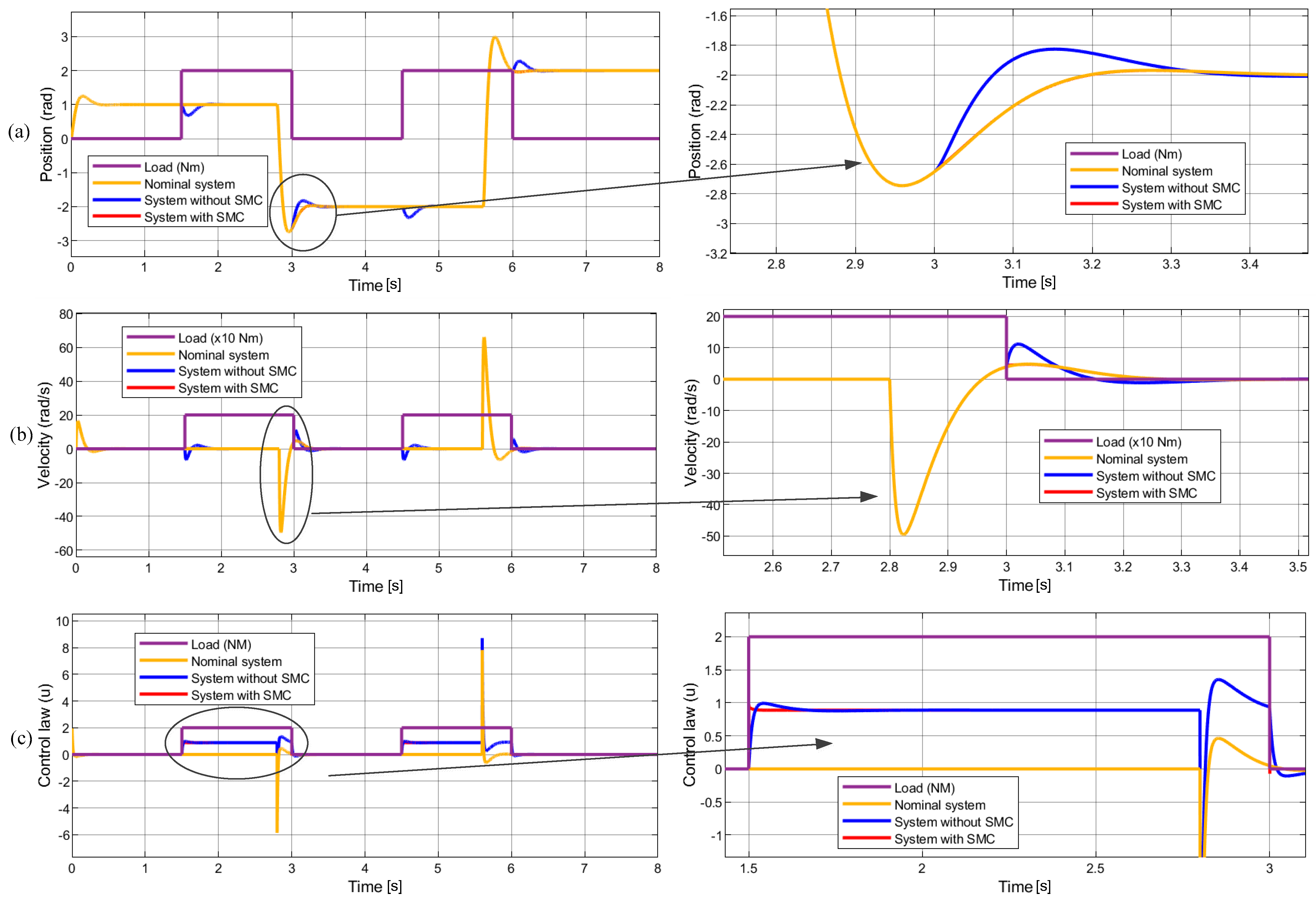
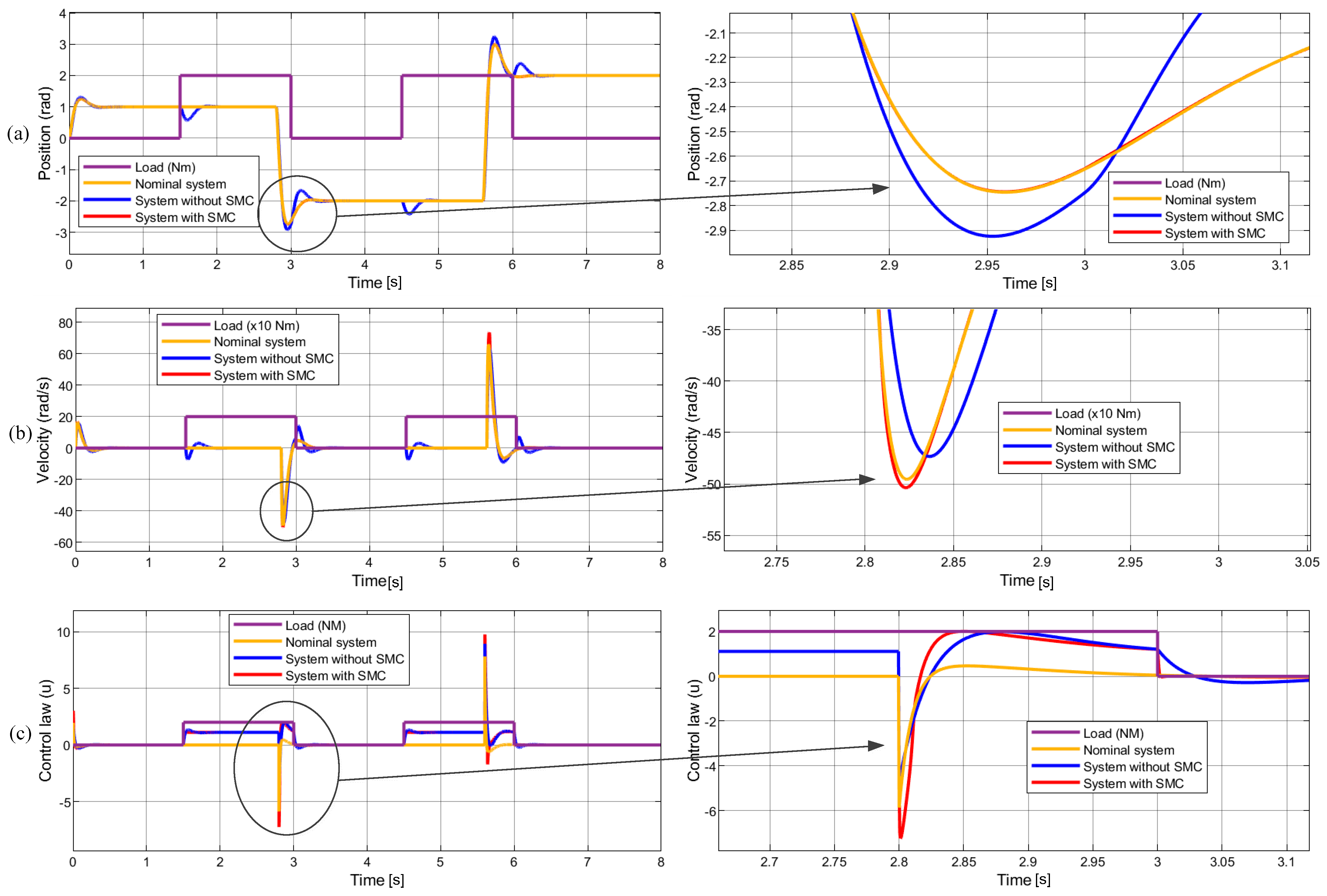
6. Simulation Results and Discussion

6.1. Simulations for Systems under the Conditions of Nominal, Load, and Uncertainty

MATLAB/Simulink was used to create a position control system, as shown in Figure 4. The motor parameters of inertia, viscous friction, and torque constant in the nominal condition are respectively $J_m=0.002 \mathrm{N}\mathrm{m}/{\mathrm{s}}^2$, $B_m=0.0015 \mathrm{N}\mathrm{m}/\mathrm{s}$, and $K_t=2.25 \mathrm{N}\mathrm{m}/\mathrm{A}$ [34]. The uncertainties of $J_m$ and $B_m$ are in the range [−50%, +50%] of their nominal values and [−20%, 0] for the torque constant. The details are shown in

Table 1. The parameters of the simulated system.

Parameter Name	Value	Variation Range
Inertia $J_m$ ($\mathrm{N}\mathrm{m}/{\mathrm{s}}^2$)	0.002	[−0.001, +0.001]
Viscous friction $B_m$ ($\mathrm{N}\mathrm{m}/\mathrm{s}$)	0.0015	[−0.00075, 0.00075]
Torque constant $K_t$ (Nm/A)	2.25	[−0.45, 0]
Feedback gain $k_1$	[−17.7778, −1.9556, −0.1060]
q	3
Position/speed loop sampling frequency	2 kHz
External load	2 Nm

. An external load of 2 Nm is also assumed to check the robustness of the proposed controller.

The objective of the simulation system is to design the servo system with the poles at $s_{1,2}=-10\pm 10i$ and $s_3=-100$. The state feedback control gain can be determined as $k_1^{\mathrm{T}}=-[\begin{array}{ccc}-17.7778& -1.9556& -0.1060\end{array}]$, and the linear control law is:

$$u_L=k_1^{\mathrm{T}}z=-[\begin{array}{ccc}-17.7778& -1.9556& -0.1060\end{array}]z$$

(39)

With the defined ranges of uncertainties, the switching control law is set as:

$$-q\mathrm{sgn}(\sigma )=-3\frac{\sigma }{\left|\sigma \right|+0.001}$$

(40)

Figure 4 shows the simulated system where the reference input is set as [1, −2, 2, −2] rad with a sample time of 2.8 s. External load is set as [0, 2, 0, 2, 0, 0] Nm with a sample time of 1.5 s. The signals of reference input and external load can be seen in Figure 5, Figure 6 and Figure 7. Those settings are used to check the performance from the frustrations under the transient and steady-state conditions. Three control structures are compared: a nominal system (ideal system) without load and uncertainty included, a controlled system using state feedback and SMC, and a controlled system with only state feedback. Three kinds of control situations are set for comparison: the uncertain condition, the loaded condition, and the condition with both the uncertainty and load.

First, the simulated results for uncertain conditions ($J_m$ changes from 0.002 $\mathrm{N}\mathrm{m}/{\mathrm{s}}^2$ to 0.003 $\mathrm{N}\mathrm{m}/{\mathrm{s}}^2$, $B_m$ changes from 0.0015 Nm/s to 0.00225 Nm/s, and $K_t$ changes from 2.25 Nm/A to 1.8 Nm/A) are shown in Figure 5. Figure 5a is the position responses. With the increased inertia, viscous friction, and decreased torque constant, the position response is affected only at the transition of position command change. The system’s response with SMC is closer to the ideal system than the system with only the integral state feedback. Figure 5b is the speed responses, and Figure 5c is the control law. Since the system states are controlled on the sliding surface with the control law (40), it shows no chattering on the speed and position response.

In the simulated system, the default motor parameters determine the feedback gain $k_1$. Thus, the uncertainties of inertia, viscous friction, and torque constant lead to the system’s poles being relocated to the positions [−10.8087+11.5237i, −10.8087–11.5237i, −42.7344]. They differ from the original for the dominant and non-dominant poles, they show a smaller damping ratio than the ideal condition, and the non-dominant pole is closer to the complex dominant poles.

Next, the load condition is used to check the performance. A load of 2 Nm is applied to the system at 1.5 s and 4.5 s and released at 3 s and 6 s as the trace purple one shown in Figure 6a–c. The position commands are the same as the conditions shown in Figure 5. When the load is applied to the system or released from the system, it shows an undershoot or overshoot for the system controlled by integral state feedback only (without SMC), as the zoomed-in figure in Figure 6a, b shows. Since the system structure with SMC has an extra switching control force, $-q\mathrm{sgn}(\sigma )=-3\frac{\sigma }{\left|\sigma \right|+0.001}$, which leads to a system with robust performance by demonstrating a response with a small undershoot or overshoot compared to the system in which only the state feedback control is applied. They can be checked using the zoomed-in pictures in Figure 6a,b in which the traces red from the system with SMC almost overlap the nominal system, i.e., the total invariant properties of SMC are preserved.

The performance under both the parameter’s variations and load is shown in Figure 7, where the inertia uncertainty and load conditions are the same settings as in Figure 5 and Figure 6. As stated in the previous section, the system parameters determine the pole locations of the closed-loop control system. A changed system model parameter causes the system performance to differ from the ideal one. All of the changes, including the command change or load added or removed, cause the responses to be far from the ideal conditions. On the contrary, the control system with SMC compensates for those frustrations and results in good responses for both the position and speed.

For the system with SMC and integral state feedback control, once the system can be kept on the sliding surface $\sigma (t,z)=0$, this will show that the system response is very close to the desired response, i.e., its equivalent system state matrix is $A_{c1}$.

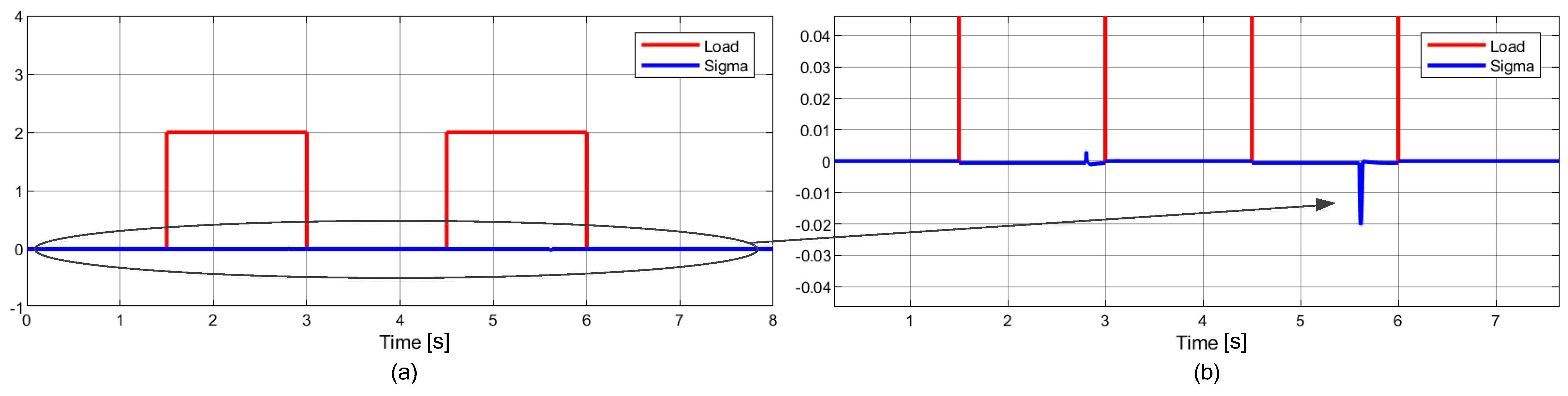
6.2. Discussion of Chattering

From the results shown in Figure 5, Figure 6 and Figure 7, those with an SMC structure have better performance than those with only integral state feedback control applied. The defined control law includes two parts: the linear part, $u_L=-k_1^{\mathrm{T}}z$, and the switching part, $u_{smc}=-q\frac{\sigma }{\left|\sigma \right|+\epsilon }$. From (27)–(29), it can be seen that the state z1 can cancel the effect from the reference input $r$ and external load $w$ in the steady state. The sliding surface $\sigma$ and the control law $u_{smc}=-q\frac{\sigma }{\left|\sigma \right|+\epsilon }$ compensate for the parameter variations’ effect. Moreover, the sliding surface usually equals 0, as Figure 8b shows, i.e., the switching control has the minimum value of q to ensure the system states, and $z$ or $x$, are kept on the sliding surface. The problem caused by the switching control and chattering is then solved.

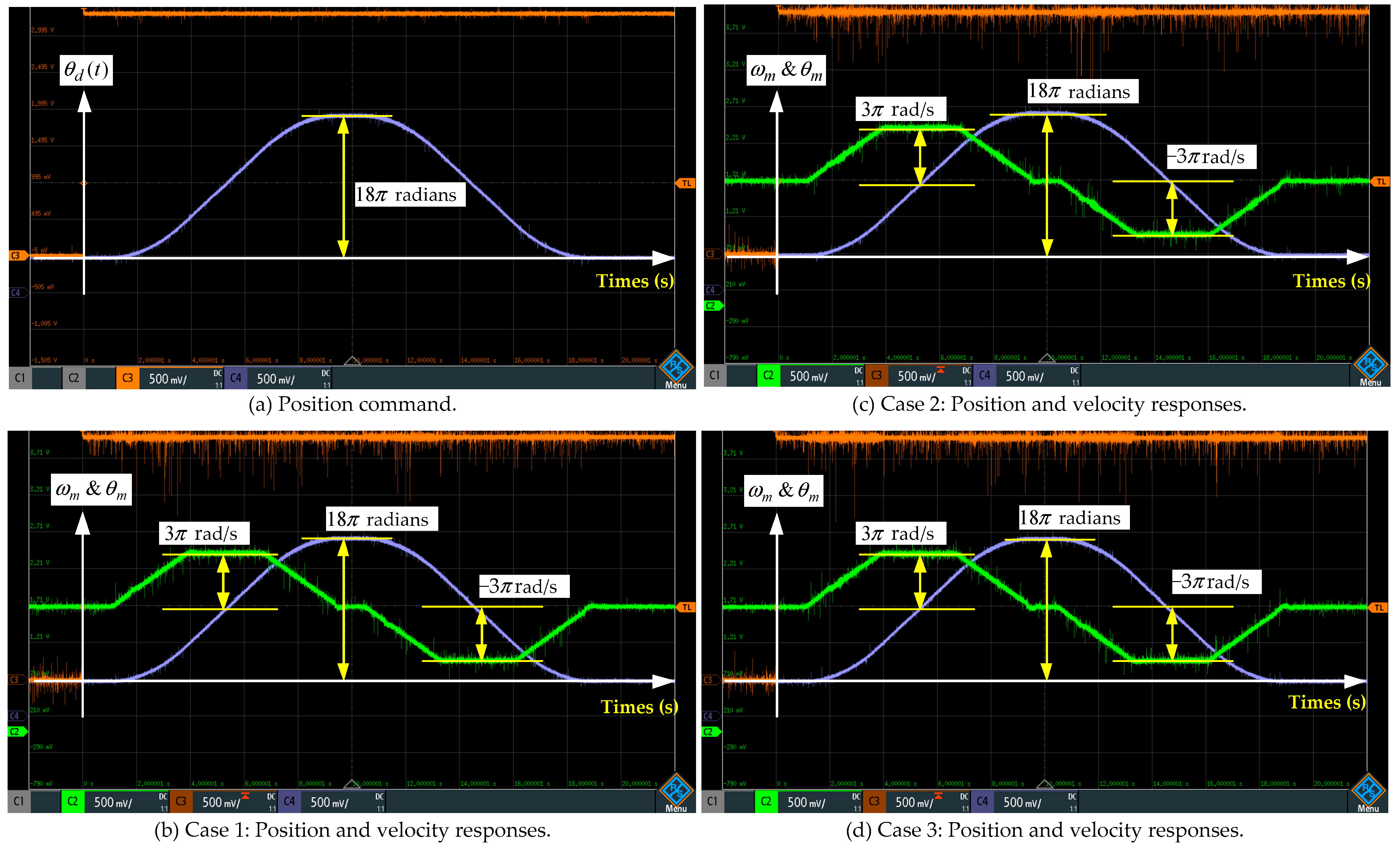
7. Practical Experiment and Discussion

The experimental system is shown in Figure 9, where the permanent magnet DC motor is axis-connected to the brake and inertia load. The brake is a piece of external voltage-controlled equipment that applies the external torque to the motor. The inertial load changes the overall system inertia by adding or removing the counterweight. The DC motor is driven by an H-bridge converter with a 24 V DC voltage source. The inner-current loop is controlled by a proportional and integral (PI)-type controller with the controller parameters $K_p=20$ and $K_i=10$ and a sampling frequency of 20 kHz. The proposed integral state feedback plus sliding mode control system controls the outer position and velocity loop. The linear control law is $u_L=-k_1^{\mathrm{T}}z=-[\begin{array}{ccc}0.7& 0.005& 0.1\end{array}]z$ and $u_{smc}=-q\frac{\sigma }{\left|\sigma \right|+\epsilon }=-3\frac{\sigma }{\left|\sigma \right|+0.001}$ and is run at a 2 kHz sampling frequency. The position and velocity signals are from the encoder with 2500 p/rev. Figure 10 is the block diagram of the developed system.

Table 2. The parameters of the practical experimental system.

Parameter Name	Value	Variation Range
$\mathrm{Normal} \mathrm{inertia} J_m(\mathrm{N}\mathrm{m}/{\mathrm{s}}^2)$	0.021675	0.01445
$\mathrm{Viscous} \mathrm{friction} B_m(\mathrm{N}\mathrm{m}/\mathrm{s})$	0.003724	0
$\mathrm{Torque} \mathrm{constant} K_t(\mathrm{N}\mathrm{m}/\mathrm{A})$	0.01041	0
$\mathrm{Feedback} \mathrm{gain} k_1$	[−0.7, −0.005, −0.1]
q	3
Position/speed loop sampling frequency	2 kHz
External load	0.002 Nm
Current PI controller	20 + 10/s
Current loop sampling frequency	20 kHz

displays the parameters of the experimental system. The controllers are implemented on the chip PIC 32 MK DSP, which works using a 120 MHz clock. Finally, the controlled parameters, position and velocity, are shown on the oscilloscope by a digital-to-analog converter (DAC). The position command is shown in Figure 11a. The total experimental time is 20 s, and the displacements are nine revolutions, which are subjected to the trapezoidal velocity profile with acceleration $\pi rad/s^2$, deceleration $-\pi rad/s^2$, and maximum speed $3\pi rad/s$. Two kinds of inertial values, which are 0.021675 $\mathrm{N}\mathrm{m}/{\mathrm{s}}^2$ and 0.036125 $\mathrm{N}\mathrm{m}/{\mathrm{s}}^2$, are built as the variations, and the brake supplies an external load of 0.002 Nm to the system periodically including 1 s ON and 2 s OFF.

Three cases are used to practically test the proposed control structure, as shown in

Table 3. The experimental setting.

Case	Conditions	External Load
1	$J_m=0.021675 \mathrm{N}\mathrm{m}/{\mathrm{s}}^2$	0
2	$J_m=0.021675 \mathrm{N}\mathrm{m}/{\mathrm{s}}^2$	0.002 Nm
3	$J_m=0.036125 \mathrm{N}\mathrm{m}/{\mathrm{s}}^2$	0.002 Nm

. Case 1 is a nominal condition with the inertia of 0.021675 $\mathrm{N}\mathrm{m}/{\mathrm{s}}^2$ and without the external load added. Case 2 is the condition with the exact inertia value, but the external load is ON and OFF control to be added to the system. In Case 3, the inertia is increased to 0.036125 $\mathrm{N}\mathrm{m}/{\mathrm{s}}^2$, and the load exists with ON and OFF control. The experimental results are shown in Figure 11b–d. They show that the controlled position and velocity responses under the perturbations still meet the required performance.

8. Conclusions

In this paper, we have demonstrated a novel controller by combining the integral state feedback control and sliding mode control to eliminate the steady-state error, improve system robustness, and allow it to have invariant properties. The method is demonstrated by a second-order system represented in controllable canonical form, and the pole placement method is applied to determine the pole position. The position control drive system is used as an example to show the design of the proposed control system. The simulation and experimental results for the nominal, load, and uncertain systems are given to verify the validity. With the proposed control structure, the problem of chattering due to the sliding mode control is solved by the integral action and boundary layer-based switching control law.

References

1. Ma’arif, A.; Setiawan, N.R. Control of DC Motor Using Integral State Feedback and Comparison with PID: Simulation and Arduino Implementation. J. Robot. Control JRC 2021, 2, 456–461. [Google Scholar] [CrossRef]
2. Kamilu, S.A.; Hakeem, M.D.A.; Olatomiwa, L. Design and Comparative Assessment of State Feedback Controllers for Position Control of 8692 DC Servomotor. Int. J. Intell. Syst. Appl. 2015, 7, 28–33. [Google Scholar] [CrossRef]
3. Al-Saggafa, U.M.; Mehedia, I.M.; Mansourib, R.; Bettayeb, M. State feedback with fractional integral control design based on the Bode’s ideal transfer function. Int. J. Syst. Sci. 2016, 47, 149–161. [Google Scholar] [CrossRef]
4. Coban, R. Backstepping integral sliding mode control of an electromechanical system. Automatika 2018, 58, 266–272. [Google Scholar] [CrossRef]
5. Herrera, M.; Leica, P.; Chavez, D.; Camacho, O. A Blended Sliding Mode Control with Linear Quadratic Integral Control based on Reduced Order Model for a VTOL System. In Proceedings of the 14th International Conference on Informatics in Control, Automation and Robotics (ICINCO 2017), Madrid, Spain, 26–28 July 2017; Volume 1, pp. 606–612. [Google Scholar]
6. Wang, W.; Zhang, J. Integral sliding mode variable structure control of DC servo motor speed. In Proceedings of the RICAI’22: Proceedings of the 2022 4th International Conference on Robotics, Intelligent Control and Artificial Intelligence, Dongguan, China, 16–18 December 2022; pp. 928–933. [Google Scholar]
7. Sanjuan, J.J.V.; Contreras, R.J.M.; Mendoza, E.Y.; Flores, J.L.; Bravo, R.O.; Tlaxcaltecatl, M.E. Design and Modeling of Integral Control State-feedback Controller for PMSM. In Proceedings of the 2018 15th International Conference on Electrical Engineering, Computing Science and Automatic Control (CCE), Mexico City, Mexico, 5–7 September 2018. [Google Scholar]
8. Templos-Santos, J.L.; Aguilar-Mejia, O.; Beltran-Carbajal, F.; Gonzalez, A.V.; Tapia-Olver, R. Integral Action in Sliding Mode Control for Reduction of Chattering in Speed Regulation of a Synchronous Motor. J. Phys. Conf. Ser. 2019, 1221, 012060. [Google Scholar] [CrossRef]
9. Baik, I.-C.; Kim, K.-H.; Youn, M.-J. Robust Nonlinear Speed Control of PM Synchronous Motor Using Boundary Layer Integral Sliding Mode Control Technique. IEEE Trans. Control Syst. Technol. 2000, 8, 47–54. [Google Scholar] [CrossRef]
10. Suh, S.; Kim, W. Position Control Based on Add-on-Type Iterative Learning Control with Nonlinear Controller for Permanent-Magnet Stepper Motors. Appl. Sci. 2021, 11, 587. [Google Scholar] [CrossRef]
11. Lai, C.-K.; Lin, B.-W.; Lai, H.-Y.; Chen, G.-Y. FPGA-Based Hybrid Stepper Motor Drive System Design by Variable Structure Control. Actuators 2021, 10, 113. [Google Scholar] [CrossRef]
12. Yu, J.; Zhuang, J.; Yu, D. State feedback integral control for a rotary direct drive servo valve using a Lyapunov function approach. ISA Trans. 2015, 54, 207–217. [Google Scholar] [CrossRef]
13. Kao, S.-T.; Chiou, W.-J.; Ho, M.-T. Integral Sliding Mode Control for Trajectory Tracking Control of an Omnidirectional Mobile Robot. In Proceedings of the 2011 8th Asian Control Conference (ASCC), Kaohsiung, Taiwan, 15–18 May 2011. [Google Scholar]
14. Jouini, M.; Dhahri, S.; Sellami, A. Combination of integral sliding mode control design with optimal feedback control for nonlinear uncertain systems. Trans. Inst. Meas. Control 2018, 41, 1331–1339. [Google Scholar] [CrossRef]
15. Gao, W.; Hung, J.C. Variable Structure Control of Nonlinear Systems: A New Approach. IEEE Trans. Ind. Electron. 1993, 40, 45–55. [Google Scholar]
16. Tanralili, A.M.R.; Al Tahtawi, A.R.; Martin. Integral State Feedback Control Design for 2-DOF Dynamixel AX-12 Manipulator Robot. In Proceedings of the 2023 10th International Conference on Information Technology, Computer, and Electrical Engineering (ICITACEE), Semarang, Indonesia, 31 August–1 September 2023. [Google Scholar]
17. Al-Baidhani, H.; Sahib, A.; Kazimierczuk, M.K. State Feedback with Integral Control Circuit Design of DC-DC Buck-Boost Converter. Mathematics 2023, 11, 2139. [Google Scholar] [CrossRef]
18. Gudey, S.K.; Gupta, R. Reduced state feedback sliding-mode current control for voltage source inverter-based higher-order circuit. IET Power Electron. 2015, 8, 1367–1376. [Google Scholar] [CrossRef]
19. Patri, K.K.; Samanta, S. State Feedback With Integral Control for Boost Converter & Its Microcontroller Implementation. In Proceedings of the 2018 IEEMA Engineer Infinite Conference (eTechNxT), New Delhi, India, 13–14 March 2018. [Google Scholar]
20. Ghosh, S.K.; Roy, T.K.; Pramanik, M.A.H.; Mahmud, M.A. Design of Nonlinear Backstepping Double-Integral Sliding Mode Controllers to Stabilize the DC-Bus Voltage for DC–DC Converters Feeding CPLs. Energies 2021, 14, 6753. [Google Scholar] [CrossRef]
21. Agrawal, N.; Samanta, S.; Ghosh, S. Optimal State Feedback-Integral Control of Fuel-Cell Integrated Boost Converter. IEEE Trans. Circuits Syst.—II Express Briefs 2022, 69, 1382–1386. [Google Scholar] [CrossRef]
22. Baghel, N.K.; Kobaku, T.; Jeyasenthil, R.; Ghorai, P.; Rajhans, C. Augmentation of State Feedback Control and Integral Action for Stabilization Issues in Islanded DC Microgrid. In Proceedings of the 2022 IEEE International Conference on Power Electronics, Drives and Energy Systems (PEDES), Jaipur, India, 14–17 December 2022. [Google Scholar]
23. Vernekar, P.; Bandal, V. Robust Sliding Mode Control of a Magnetic Levitation System: Continuous-Time and Discrete-Time Approaches. arXiv 2021, arXiv:2110.12363. [Google Scholar]
24. Yu, X.-N.; Hao, L.-Y. Integral sliding mode fault tolerant control for unmanned surface vessels with quantization: Less iterations. Ocean Eng. 2022, 260, 111820. [Google Scholar] [CrossRef]
25. Winursito, A.; Dhewa, O.A.; Nasuha, A.; Pratama, G.N.P. Integral State Feedback Controller with Coefficient Diagram Method for USV Heading Control. In Proceedings of the 2022 5th International Conference on Information and Communications Technology (ICOIACT), Yogyakarta, Indonesia, 24–25 August 2022. [Google Scholar]
26. Mahmood, A.; Bhatti, A.I.; Siddique, B.A. Landing of Aircraft Using Integral State Feedback Sliding Mode Control. In Proceedings of the 1st International Conference on Electrical, Communication and Computer Engineering (ICECCE), Swat, Pakistan, 24–25 July 2019. [Google Scholar]
27. Eltayeb, A.; Rahmat, M.F.; Basri, M.A.M.; Mahmoud, M.S. An Improved Design of Integral Sliding Mode Controller for Chattering Attenuation and Trajectory Tracking of the Quadrotor UAV. Arab. J. Sci. Eng. 2020, 45, 6949–6961. [Google Scholar] [CrossRef]
28. Seeber, R.; Tranninger, M. Integral state-feedback control of linear time-varying systems: A performance preserving approach. Automatica 2022, 136, 110000. [Google Scholar] [CrossRef]
29. Shyu, K.-K.; Hung, J.C. Totally invariant variable structure control systems. In Proceedings of the IECON’97 23rd International Conference on Industrial Electronics, Control, and Instrumentation, New Orleans, LA, USA, 14 November 1997. [Google Scholar]
30. Behera, A.K.; Bandyopadhyay, B.; Spurgeon, S.K. Arbitrary Pole Placement with Sliding Mode Control. In Proceedings of the 2022 16th International Workshop on Variable Structure Systems (VSS), Rio de Janeiro, Brazil, 11–14 September 2022. [Google Scholar]
31. Ali, H.I.; Abdulridha, A.J. State Feedback Sliding Mode Controller Design for Human Swing Leg System. Al-Nahrain J. Eng. Sci. 2018, 21, 51–59. [Google Scholar] [CrossRef]
32. Bhaskarwar, T.; Hawari, H.F.; Nor, N.B.M.; Chile, R.H.; Waghmare, D.; Aole, S. Sliding Mode Controller with Generalized Extended State Observer for Single Link Flexible Manipulator. Appl. Sci. 2022, 12, 3079. [Google Scholar] [CrossRef]
33. Franklin, G.F.; Powell, J.D.; Workman, M. Digital Control of Dynamic Systems, 3rd ed.; Addison Wesley Longman, Inc.: Menlo Park, CA, 1998. [Google Scholar]
34. Lai, C.-K.; Shyu, K.-K. A Novel Motor Drive Design for Incremental Motion System via Sliding-Mode Control Method. IEEE Trans. Ind. Electron. 2005, 52, 499–507. [Google Scholar] [CrossRef]
Figure 1. The control block diagram of state feedback.
Applsci 14 01083 g001
Figure 2. The control block diagram of the augmented system.
Applsci 14 01083 g002
Figure 3. The block diagram of the second-order controlled system.
Applsci 14 01083 g003
Figure 4. The simulation system.
Applsci 14 01083 g004
Figure 5. The system’s responses with parameter uncertainty: (a) position, (b) velocity, and (c) control law.
Applsci 14 01083 g005
Figure 6. The system’s responses with load: (a) position, (b) velocity, and (c) control law.
Applsci 14 01083 g006
Figure 7. The system’s responses with load and uncertainty: (a) position; (b) velocity; and (c) control law.
Applsci 14 01083 g007
Figure 8. The sliding surface and load: (a) original picture and (b) zoomed-in picture in the vicinity of 0.
Applsci 14 01083 g008
Figure 9. The experimental platform for the DC motor drive system.
Applsci 14 01083 g009
Figure 10. The block diagram of the motor drive system.
Applsci 14 01083 g010
Figure 11. The experimental results: (a) the position command; (b) Case 1; (c) Case 2; and (d) Case 3.
Applsci 14 01083 g011